Distributed Adaptive Optimization Algorithm for Fractional High-Order Multiagent Systems Based on Event-Triggered Strategy and Input Quantization

Abstract

This paper investigates the distributed optimization problem (DOP) for fractional high-order nonstrict-feedback multiagent systems (MASs) where each agent is multiple-input–multiple-output (MIMO) dynamic and contains uncertain dynamics. Based on the penalty-function method, the consensus constraint is eliminated and the global objective function is reconstructed. Different from the existing literatures, where the DOPs are addressed for linear MASs, this paper deals with the DOP through using radial basis function neural networks (RBFNNs) to approximate the unknown nonlinear functions for high-order MASs. To reduce transmitting and computational costs, event-triggered scheme and quantized control technology are combined to propose an adaptive backstepping neural network (NN) control protocol. By applying the Lyapunov stability theory, the optimal consensus error is proved to be bounded and all signals remain semi-global uniformly ultimately bounded. Simulation shows that all agents reach consensus and errors between agents’ outputs and the optimal solution is close to zero with low computational costs.

1. Introduction

Recently, distributed optimization problem (DOP) of MASs has attracted much interest since its wide range applications including robotic systems [1,2], sensor networks [3], marine surface vehicles [4], smart grids [5,6], fractional order MASs [7] and multiple one-link manipulators system [8]. Given a DOP, each agent acquires a local objective function and the MASs have a global objective function obtained by making the sum of local objective functions. Through minimizing the global objective function, agents in MASs follow an optimal trajectory while reaching consensus.

A key objective for the DOP is to provide appropriate distributed control algorithms which ensure that all agents in MASs collaborate in seeking the optimal solution of the global objective function. Ref. [9] designs a discrete algorithm for multi-robot system to deal with the cooperative transportation by minimizing the total energy consumption. In [10], a class of online DOP considering coupled inequality constraints is investigated and an online primal-dual algorithm is developed. Noting that the above papers focus on the development of discrete-time algorithm for DOP, which means these algorithms are not suitable for the continuous-time dynamics. Recently, a growing number of researchers are developing continuous-time algorithms for DOP due to its potential applications in MASs [11,12,13,14,15]. In [16], a distributed algorithm is developed to deal with the resource allocation problem by designing a dynamic event-triggered mechanism. On the basis of proportional integral technique, Ref. [17] proposes an adaptive neurodynamic algorithm to address the DOP and the proposed algorithm ensures that agents in MASs achieve consensus first in a finite-time and then converge to the optimal trajectory in a fixed-time. To avoid solving high-dimensional subproblems, Ref. [18] proposes a novel projection-free dynamics for solving constrained DOP using the Frank–Wolfe method. An adaptive fault-tolerant controller is designed in [19] to deal with the DOP for nonlinear MASs through building exosystem state observers. In these research works, algorithms are developed for DOPs in first-order MASs, which means that in second-order MASs, these methods are hardly to work well. With this reason in mind, many methods are constructed for second-order MASs due to the widely use in practice [20,21,22,23]. In [24], a decentralized optimization control protocol with fixed-time flocking is developed for second-order MASs where the networks are time-varying. Ref. [25] develops a dynamic event-trigger based control protocol for the optimal consensus problem in second-order MASs where communication edges are affected by both cyber attacks and disturbances simultaneously. The generic optimal formation control problems with various formation constraints is investigated in [26] for second-order MASs. In many engineering practices, such as generators, robots, and satellites, the dynamics of physical systems can be depicted by high-order systems. Thus, investigating the DOP in high-order MASs is meaningful and important. However, due to the inaccuracy of modeling, many MASs contains nonlinear uncertainties objectively and the aforementioned algorithms may be ineffective.

To address this issue, many adaptive methods, such as RBFNNs and fuzzy logic systems (FLSs), are adopted to compensate for the unknown nonlinear function and design an adaptive control protocol to achieve the control goal. Through ultilizing RBFNNs or FLSs, a wide range of adaptive control protocols are developed [27,28,29,30]. In [31], an adaptive control protocol is proposed based on FLSs technique to address the switched nonlinear functions in the MIMO system and the unknown gain direction of the controller is solved by the Nussbaum gain function. To reduce computation, a RBFNNs-based prescribed- time controller is developed in [32] via event-trigger mechanism for robotic manipulators with nonlinear uncertainties and state constraints. In [33], based on the projection operator-based compensation mechanism, a FLSs-based adaptive controller is proposed to deal with the consensus problem in nonlinear MASs under deception attacks. Upon reviewing the above literature, it should be noted that there is currently no study on developing the adaptive intelligent control protocol for the high-order uncertain nonstrict-feedback MASs with MIMO agents. Besides, as a special case of consensus problems, DOP needs all agents to achieve both consensus and the optimal solution, which means that the aforementioned algorithms may not work to realize the control objective.

Furthermore, the above studies are restricted to integer-order MASs only. In reality, fractional-order MASs (FOMASs) have multiple potential applications due to its ability to accurately model the system [34,35]. Recently, the consensus problem for FOMASs has attracted considerable attention and has emerged as another research priority [36,37,38,39]. Ref. [40] introduces an adaptive algorithm using an event-triggered strategy for FOMASs with partial state constraints and input saturation. Ref. [41] develop a novel distributed algorithm with fixed time delay to address containment control problem for nonlinear FOMASs. However, to the best of our knowledge, the DOP for uncertain nonlinear FOMASs where each agent is described by MIMO dynamics has not been studied in the existing works. This motivates us to undertake the research in this paper.

Motivated by the above discussion, this paper proposes an event-trigger based adaptive backstepping algorithm to address the DOP using input quantization technique for the nonstrict-feedback MIMO MASs. The main contributions in this paper are as follow.

(1)

Unlike [27,33], where algorithms are developed for the consensus problem in MASs, this paper introduces an adaptive control protocol for the DOP. Agents in the MASs not only reach consensus, but also achieve the optimal solution of the global objective function. Besides, each agent in the FOMASs is described by nonstrict-feedback MIMO dynamics, which is more general and complex to design the control protocol.

(2)

Different from [16,17,18,19,20,21,22,23,24,25,26], where the DOPs are investigated for first-order or second-order MASs, this paper dedicates to solve the fractional high-order DOP, which means that MASs and the DOP in this paper are close to the engineering systems. Besides, the MASs in this paper includes nonlinear uncertain terms in each order. Thus, RBFNNs technique is adopted to approximate and compensate for the unknown dynamics. In addition, to reduce the transmitting and computational costs, this paper combines the event-trigger mechanism and input quantization technique together to deal with the high-order DOP for the first time.

(3)

In contrast to the algorithms in aforementioned works which are only effective in integer order MASs, this paper investigates the high-order DOP in uncertain nonlinear FOMASs with MIMO agents and an adaptive NNs based algorithm is developed. To avoid the ’computation complexity’, this paper utilizes the fractional order DSC (FODSC) method and the fractional derivatives for virtual controllers are obtained in the meantime.

2. Preliminaries

Define the Caputo fractional derivative [42] as

$$\begin{array}{c}\hfill {}_0^C{D}_t^{\omega }f\left(t\right)=\frac{1}{\mathrm{\Gamma }\left(\delta -\omega \right)}{\int }_0^t\frac{f^{\left(\delta \right)}\left(\tau \right)}{{\left(t-\tau \right)}^{1+\omega -\delta }}d\tau \end{array}$$

where $\delta \in \Delta$ and $\delta -1<\omega \le \delta$, $\mathrm{\Gamma }\left(z\right)={\int }_0^{\infty }{t}^{z-1}{e}^{-t}dt$ is the Gamma function. In this paper, we set ${}_0^C{D}_t^{\omega }f\left(t\right)=D^{\omega }f\left(t\right)$ to simplify the notation. For a two-parameter function of the Mittag-Leffler type

$$\begin{array}{c}\hfill E_{\omega ,\gamma }\left(\varsigma \right)=\sum _{n=0}^{\infty }\frac{{\varsigma }^n}{\mathrm{\Gamma }(\omega n+\gamma )},(\omega >0),(\gamma >0)\end{array}$$

we have the following lemmas.

Lemma 1

([43]). For real numbers γ, ω and ϕ satisfying $\omega \in \left(0,1\right)$, $\tau >0$, one has

$$\frac{\tau \omega }{2}<\varphi <\tau \omega$$

(1)

and for integers $n\ge 1$, one obtains

$$E_{\omega ,\gamma }\left(\varsigma \right)=-\sum _{j=1}^n\frac{{\varsigma }^{-j}}{\mathrm{\Gamma }\left(\gamma -\omega j\right)}+o\left(\frac{1}{{\left|\varsigma \right|}^{n+1}}\right)$$

(2)

when $\left|\varsigma \right|\to \infty ,\varphi \le \left|arg\left(\varsigma \right)\right|\le \tau$.

Lemma 2

([43]). If ϕ satisfies the condition of Lemma 1, one holds

$$\begin{array}{c}\hfill \left|E_{\omega ,\gamma }\left(\varsigma \right)\right|\le \frac{\mu }{1+\left|\varsigma \right|}\end{array}$$

where $\omega \in \left(0,2\right)$ and γ is an arbitrary real number, $\mu >0$, $\varphi \le \left|arg\left(\varsigma \right)\right|\le \tau$.

Lemma 3

([44]). For $\kappa \in R$ and $\zeta >0$, the following inequality holds

$$\begin{array}{c}\hfill 0\le \left|\kappa \right|-\frac{{\kappa }^2}{\sqrt{{\kappa }^2+{\zeta }^2}}\le \zeta \end{array}$$

Lemma 4

([42]). Suppose that the Lyapunov function $V\left(t,x\right)$ satisfies $D^{\omega }V\left(t,x\right)\le -\mathrm{\Theta }V\left(t,x\right)+\mathrm{\Lambda }$. Let $0<\omega <1$, $\mathrm{\Theta }>0$ and $\mathrm{\Lambda }\ge 0$, the following inequality holds

$$\begin{array}{c}\hfill \begin{array}{cc}V\left(t,x\right)\le V\left(0\right)E_{\omega }\left(-\mathrm{\Theta }{t}^{\omega }\right)+\frac{\mathrm{\Lambda }\mu }{\mathrm{\Theta }},& t\ge 0\end{array}\end{array}$$

Then, $V\left(t,x\right)$ is bounded on $\left[0,t\right]$ and fractional order systems are stable, where $\mu$ is defined in Lemma 2.

Notations: In this paper, ${\mathbf{0}}_m={[0,\dots ,0]}^T\in R^m$, ${\mathbf{1}}_m={[1,\dots ,1]}^T\in R^m$. Denote $\nabla f(·)$ as the gradient of function $f(·)$ and ⊗ as Kronecker product.

Remark 1.

In this paper, the fractional order is considered within the interval $[0,1]$.

3. Problem Formulation

3.1. Hysteresis Quantizer

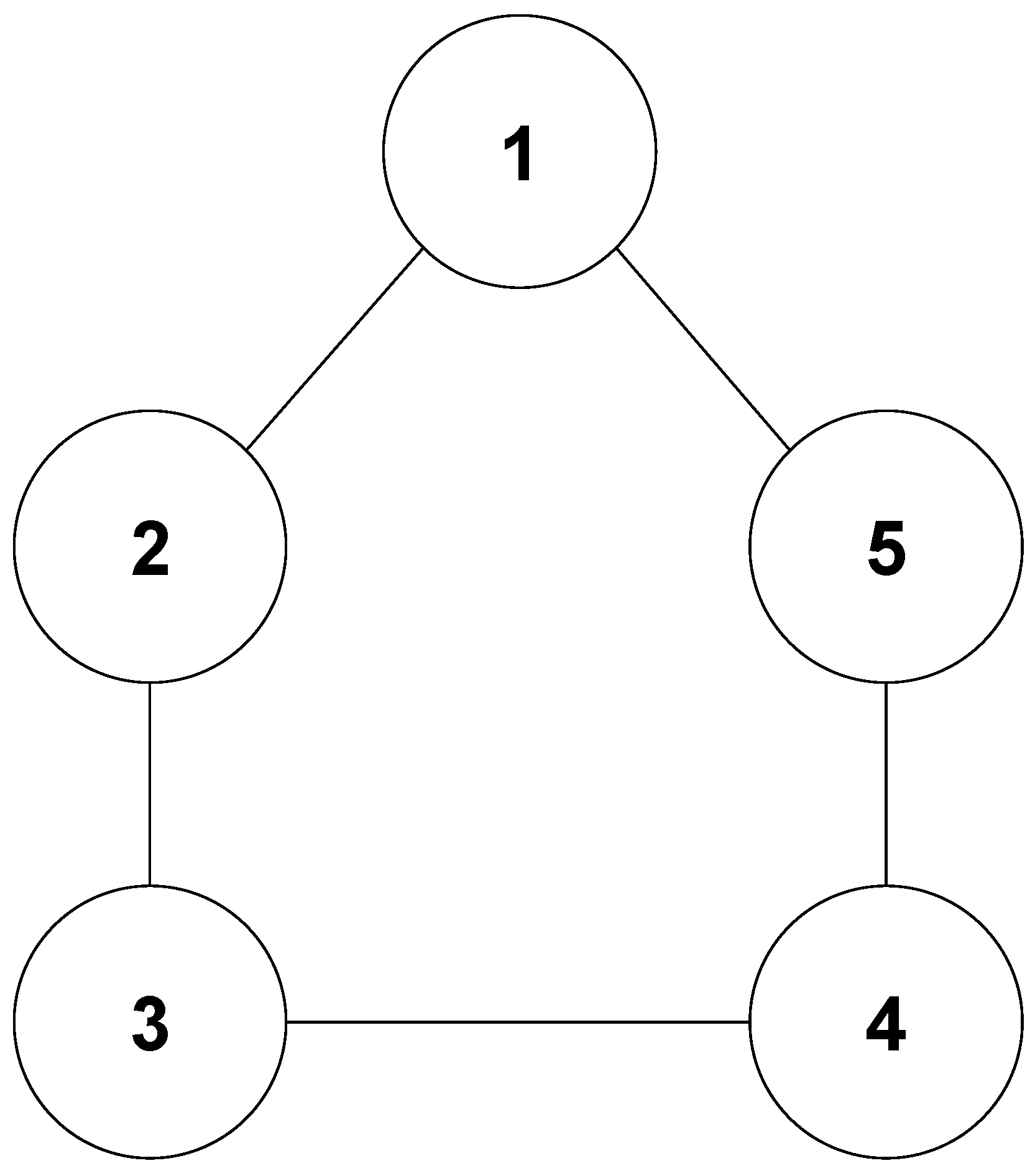
This paper uses the hysteresis quantizer to reduce chattering. According to [45], the quantizer ${\upsilon }_i\left({\varpi }_i\left(t\right)\right)$ is

$${\upsilon }_i\left({\varpi }_i\left(t\right)\right)=\left\{\begin{array}{c}{\varpi }_{ik}sign\left({\varpi }_i\right),\hfill \\ {\varpi }_{ik}\left(1+d\right)sign\left({\varpi }_i\right),\hfill \\ 0,\hfill \end{array}\right.\begin{array}{c}\frac{{\varpi }_{ik}}{1+d}<\left|{\varpi }_i\right|\le \frac{{\varpi }_{ik}}{1-d}\\ {\varpi }_{ik}<\left|{\varpi }_i\right|\le \frac{{\varpi }_{ik}\left(1+d\right)}{1-d}\\ 0\le \left|{\varpi }_i\right|<{\varpi }_{min}\end{array}$$

(3)

where ${\varpi }_{ik}=n^{1-k}{\varpi }_{min}\left(k=1,2,\dots \right)$ with parameters ${\varpi }_{min}>0$ and $0<\varrho <1$, $d=\frac{1-\varrho }{1+\varrho }$. Meanwhile, ${\upsilon }_i\left({\varpi }_i\left(t\right)\right)$ is in the set $U=\left[0,\pm {\varpi }_{ik},\pm {\varpi }_{ik}\left(1+d\right)\right],k=1,2,\dots$. ${\varpi }_{min}$ determines the magnitude of the dead-zone for ${\upsilon }_i\left({\varpi }_i\left(t\right)\right)$.

Lemma 5

([46]). The system inputs ${\upsilon }_i\left({\varpi }_i\left(t\right)\right)$ can be described as

$${\upsilon }_i\left({\varpi }_i\left(t\right)\right)=\mathrm{\Xi }\left({\varpi }_i\right){\varpi }_i\left(t\right)+{\mathrm{\Psi }}_i\left(t\right)$$

(4)

where $1-d\le \mathrm{\Xi }\left({\varpi }_i\right)\le 1+d$, $\left|{\mathrm{\Psi }}_i\left(t\right)\right|\le {\varpi }_{min}$.

3.2. Graph Theory

Denote an undirected graph $\mathcal{Q}=\left(\mathcal{U},\mathcal{J},\overline{A}\right)$, where $\mathcal{U}=\left\{1,\dots ,N\right\}$ is a node set. Define $\mathcal{J}\subset \mathcal{U}\times \mathcal{U}$ as the edge set with no self-loop and $\overline{A}=\left\{a_{ij}\right\}\in R^{N\times N}$ as the adjacency matrix. An edge $(i,j)\in \mathcal{J}$, if and only if $a_{ij}=1$. Denote $N_i=\left\{j\left|\right(i,j)\in \mathcal{J}\right\}$ as the neighbor set of node i and the matrix $D=diag\left\{{\sum }_{j=1}^N{a}_{1j},\dots ,{\sum }_{j=1}^N{a}_{Nj}\right\}$ as the degree matrix. Define the Laplacian matrix as $L=D-\overline{A}$. If there is an undirected path between each node pair, graph $\mathcal{Q}$ is a connected graph.

Lemma 6

([47]). For a connected undirected graph Q, it has a positive semi-definite Laplacian matrix which has a simple eigenvalue 0 and the associated eigenvector ${\mathbf{1}}_N$.

3.3. Multi-Agent Systems

Consider the FOMASs with N agents and each agent is described by the MIMO system with m subsystems. The dynamic for agent i is:

$$\left\{\begin{array}{cc}\hfill D^{\alpha }{x}_{i,l}\left(t\right)& =x_{i,l+1}+h_{i,l}\left(X_{i,n}\right)\hfill \\ \hfill D^{\alpha }{x}_{i,n}\left(t\right)& =u_i\left(t\right)+h_{i,n}\left(X_{i,n}\right)\hfill \\ \hfill y_i& =x_{i,1}\hfill \end{array}\right.$$

(5)

where $i=1,\dots ,N$, $l=1,\dots ,n-1$, $\alpha \in \left(0,1\right)$, $x_{i,1},\dots ,x_{i,l}\in R^m$ are system states, $u_i\left(t\right)\in R^m$ is the control input, $y_i={[y_{i,1},\dots ,y_{i,m}]}^T\in R^m$ is the system output, $X_{i,n}={[x_{i,1}^T,\dots ,x_{i,n}^T]}^T$$\in R^{mn}$ is the state vector, $h_{i,l}\left(X_{i,n}\right)={[h_{i,l,1}\left(X_{i,n}\right),\dots ,h_{i,l,m}\left(X_{i,n}\right)]}^T\in R^m$ is the vector of unknown nonlinear functions. Specifically, the kth subsystem is described as

$$\left\{\begin{array}{cc}\hfill D^{\alpha }{x}_{i,l,k}\left(t\right)& =x_{i,l+1,k}+h_{i,l,k}\left(X_{i,n}\right)\hfill \\ \hfill D^{\alpha }{x}_{i,n,k}\left(t\right)& =u_{i,k}\left(t\right)+h_{i,n,k}\left(X_{i,n}\right)\hfill \\ \hfill y_{i,k}& =x_{i,1,k}\hfill \end{array}\right.$$

(6)

where $x_{i,l,k}$ is the system state, $y_{i,k}$ is the system output, $u_{i,k}\left(t\right)$ is the control input, $h_{i,l,k}\left(X_{i,n}\right)$ is an unknown nonlinear function.

3.4. Distributed Optimization Problem

This paper investigates the quadratic DOP for the FOMASs. For agent i, define the local objective function $f_i(·):R^m\to R$ as

$$\begin{array}{c}\hfill f_i\left(y_i\right)=y_i^T{a}_i\left(t\right)y_i+b_i^T\left(t\right)y_i+c_i\left(t\right)\end{array}$$

(7)

where $a_i\left(t\right)\in R^{m\times m}$, $b_i\left(t\right)\in R^m$, $c_i\left(t\right)\in R^m$, $∥a_i\left(t\right)∥\le a_0$, $∥b_i\left(t\right)∥\le b_0$, $∥c_i\left(t\right)∥\le c_0$ and $a_0$, $b_0$, $c_0$ are known constants. The global objective function $f(·):R^{mN}\to R$ is defined as

$$\begin{array}{cc}\hfill & f\left(y\right)=\sum _{i=1}^N{f}_i\left(y_i\right)\hfill \\ & s.t.(L\otimes I_m)y={\mathbf{0}}_{mN}\hfill \end{array}$$

(8)

where $y={[y_1^T,\dots ,y_N^T]}^T$. According to Lemma 6, given a bounded continuous function $\alpha \left(t\right)$, if $y=\alpha \left(t\right)·{\mathbf{1}}_{mN}$, one has $(L\otimes I_m)y=0$. Thus, based on the penalty-function method, design the penalty term $\frac{1}{2}\mu y^T(L\otimes I_m)y$ where $\mu$ is a positive designed parameter. The global objective function can be rewritten as

$$\begin{array}{c}\hfill F\left(y\right)=\sum _{i=1}^N{f}_i\left(y_i\right)+\frac{1}{2}\mu y^T(L\otimes I_m)y\end{array}$$

(9)

Define the optimal solution of $F\left(y\right)$ as $y_{*}={[y_{1*}^T,\dots ,y_{N*}^T]}^T\in R^{mN}$ and $y_{*}=\underset{(y_1,\dots ,y_N)}{argmin}F\left(y\right)$, where $y_{i*}={[y_{i,1*},\dots ,y_{i,m*}]}^T$. From (9), we know that when the FOMASs achieve the optimal solution $y_{*}$, all agents reach consensus and converge to the optimal trajectory simultaneously.

Control objectives: This paper aims at developing an adaptive NNs-based control protocol using FODSC technology, event-trigger mechanism and input quantization, so that all agents’ signals remain bounded and converge to the optimal trajectory while keeping consensus with sufficiently small errors.

4. Main Results

4.1. Neural Networks Approximation

As an effective tool for approximating continuous functions, RBFNNs in this paper are utilized to compensate for the nonlinear functions $h\left(X_{i,n}\right):R^n\to R$. The RBFNNs are described as follow

$$\begin{array}{c}\hfill h\left(X_{i,n}\right)={\vartheta }^T\phi \left(X_{i,n}\right)\end{array}$$

(10)

where $X_{i,n}\in R^{mn}$ is the input vector, $\vartheta \in R^p$ is the weight vector and $\phi \left(X_{i,n}\right)=[{\phi }^1\left(X_{i,n}\right),\dots ,$${\phi }^p\left(X_{i,n}\right){]}^T\in R^p$ is the radial basis function vector and p represents the NN nodes where ${\phi }^q\left(X_{i,n}\right)$ is a typical basis Gaussian function as

$$\begin{array}{c}\hfill {\phi }^q\left(X_{i,n}\right)=exp\left[\frac{-{(X_{i,n}-c_q)}^T(X_{i,n}-c_q)}{b_q^2}\right],q=1,\dots ,p\end{array}$$

(11)

with $c_q\in R^n$ being the centers and $b_q\in R$ being the width of Gaussian functions.

Lemma 7

([36]). Given a continuous unknown function $h\left(x\right)$ defined on the compact set ${\mathrm{\Omega }}_x$, there exist the NN ${\vartheta }^{*T}\phi \left(x\right)$ and the arbitrary accuracy $ϵ\left(x\right)$ such that

$$\begin{array}{c}\hfill h\left(x\right)={\vartheta }^{*T}\phi \left(x\right)+ϵ\left(x\right)\end{array}$$

(12)

where ${\vartheta }^{*}$ is the ideal weight vector defined by ${\vartheta }^{*}={argmin}_{\vartheta \in {\mathrm{\Omega }}_{\vartheta }}\left[{sup}_{x\in {\mathrm{\Omega }}_x}\right|h\left(x\right)-{\vartheta }^T\phi \left(x\right)]$ defined by ϑ and $ϵ\left(x\right)$ denotes the minimum approximation error.

Define the parameter estimation error $\tilde{\vartheta }$ and the optimal approximation error ϵ as

$$\tilde{\vartheta }={\vartheta }^{*}-\vartheta ,l=1,2,\dots ,n.$$

(13)

$$ϵ=h\left(X_{i,n}\right)-h\left(X_{i,n}\right|{\vartheta }^{*})$$

(14)

where $h\left(X_{i,n}\right|{\vartheta }^{*})$ is the arrpoximation value of RBFNNs with the optimal parameter.

Assumption 1.

The optimal approximation errors remain bounded and the arbitrary accuracy satisfies $ϵ\left(x\right)\le {ϵ}_0$, ${ϵ}_0>0$.

4.2. Controller Design

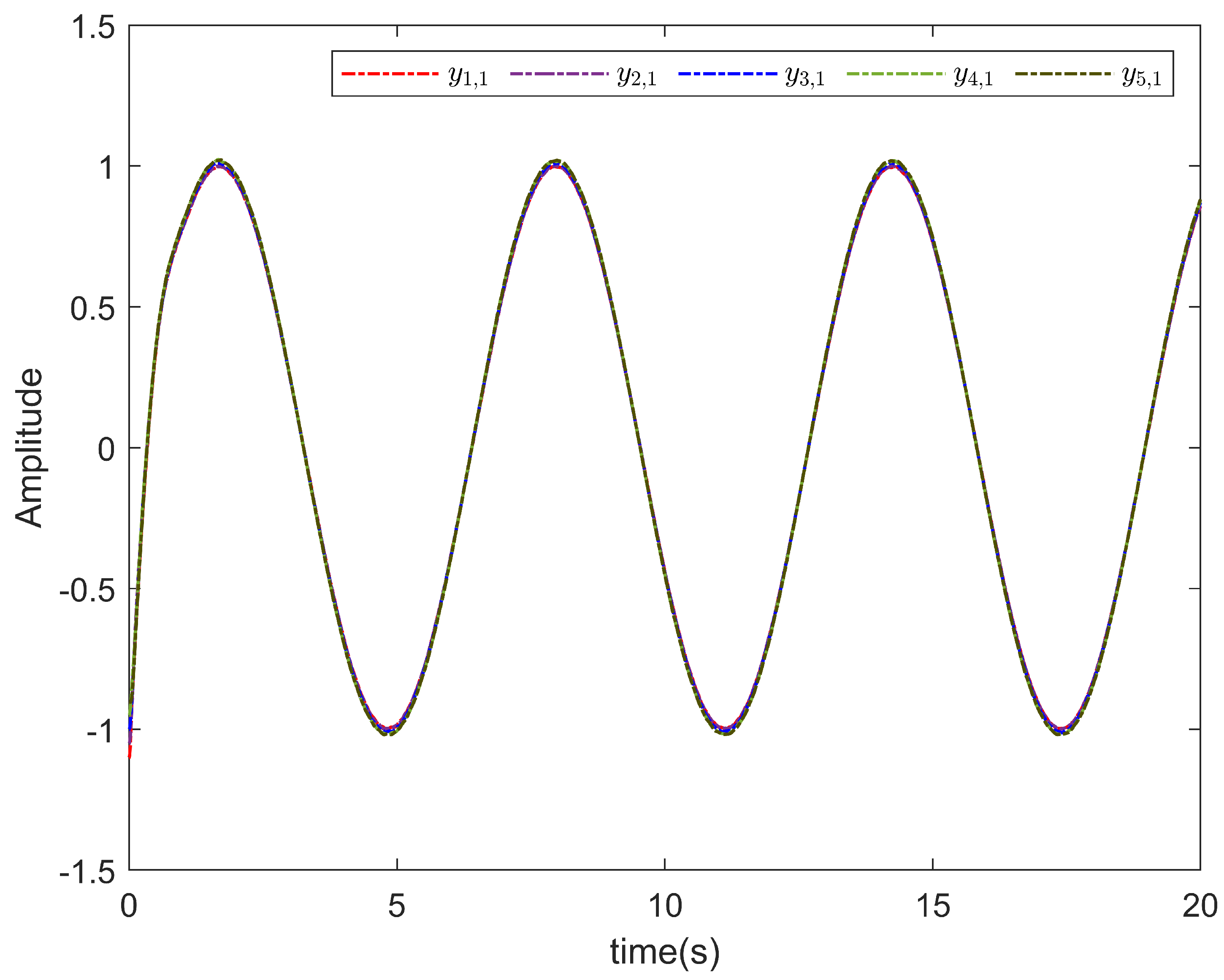
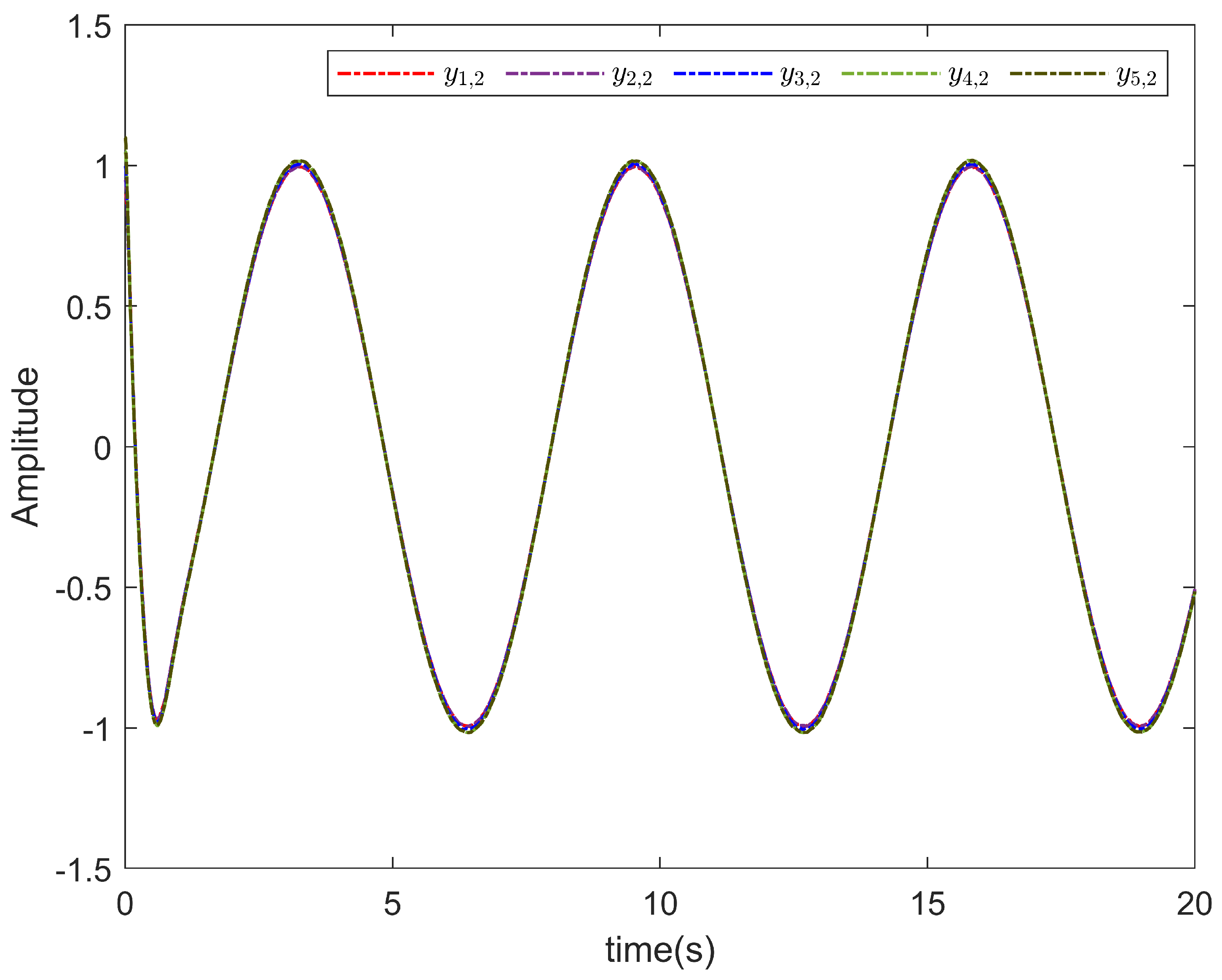
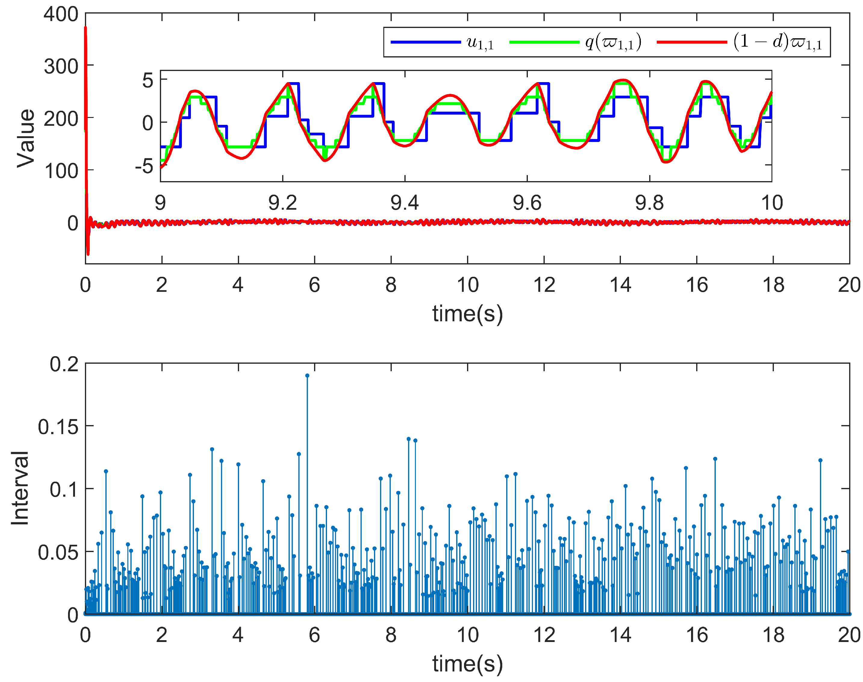
Theorem 1.

For the nonlinear FOMASs under Assumption 1, we construct an event-trigger adaptive NN-based dynamic surface quantized controller (70), virtual controllers (29), (41) and (55), adaptive laws (30), (42), (56) and (67) such that all signals in the closed-loop system remain semi-global uniformly ultimately bounded and errors between outputs and the optimal trajectory are sufficiently small.

Proof. 

Define the errors for agent i, subsystem k as follow

$$\begin{array}{cc}\hfill & z_{i,1,k}=x_{i,1,k}-y_{i,k}^{*}\hfill \\ & z_{i,l,k}=x_{i,l,k}-r_{i,l,k}\hfill \\ & w_{i,l,k}=r_{i,l,k}-x_{i,l,k}^{*}\hfill \\ & l=2,\cdots ,nk=1,\cdots ,m\hfill \end{array}$$

(15)

where $z_{i,1,k}$ is the tracking error, $r_{i,l,k}$ is the output of the FODSC, and $w_{i,l,k}$ is the FODSC error between $r_{i,l,k}$ and $x_{i,l,k}^{*}$.

Step 1. According to (7) and (9), the gradient of newly constructed global objective function $F\left(y\right)$ is

$$\begin{array}{cc}\hfill \nabla F\left(y\right)=& \frac{\partial {\sum }_{i=1}^N{f}_i\left(y_i\left(t\right)\right)}{\partial y}+\mu (L\otimes I_m)y.\hfill \end{array}$$

(16)

Since the global objective function $F\left(y\right)$ is convex, the optimal solution $y_{*}$ satisfies $\nabla F\left(y_{*}\right)=0$. Thus, for agent i, we obtain

$$2a_i\left(t\right)y_{i_{*}}+b_i\left(t\right)+\mu \sum _{j\in N_i}^{}{a}_{ij}(y_{i*}-y_{j*})={\mathbf{0}}_m.$$

(17)

Define the vector $z_{i,1}={[z_{i,1,1},\dots ,z_{i,1,m}]}^T$. From (13) and (15), one has

$$\begin{array}{cc}\hfill \frac{\partial F\left(y\right)}{\partial y_i}=& \frac{\partial f_i\left(y_i\left(t\right)\right)}{\partial y_i}+\mu \sum _{j\in N_i}^{}{a}_{ij}(y_i-y_j)\hfill \\ \hfill =& 2a_i\left(t\right)y_i+b_i\left(t\right)+\mu \sum _{j\in N_i}^{}{a}_{ij}(y_i-y_j)\hfill \\ \hfill =& 2a_i\left(t\right)y_i+b_i\left(t\right)+\mu \sum _{j\in N_i}^{}{a}_{ij}(y_i-y_j)-2a_i\left(t\right)y_{i*}-b_i\left(t\right)-\mu \sum _{j\in N_i}^{}{a}_{ij}(y_{i*}-y_{j*})\hfill \\ \hfill =& 2a_i\left(t\right)z_{i,1}+\mu \sum _{j\in N_i}^{}{a}_{ij}(z_{i,1}-z_{j,1}).\hfill \end{array}$$

(18)

Let $z_1={[z_{1,1}^T,\dots ,z_{N,1}^T]}^T$. Through (16) and (18), one obtains

$$\frac{\partial F\left(y\right)}{\partial y}=H{z}_1$$

(19)

where $H=A+\mu (L\otimes I_m)$ and $A=2diag\left\{a_i\left(t\right)\right\}$. Construct the Lyapunov function for FOMASs as:

$$\begin{array}{cc}\hfill V_1& =\frac{1}{2}{\left(\frac{\partial F\left(y\right)}{\partial y}\right)}^T{H}^{-1}\left(\frac{\partial F\left(y\right)}{\partial y}\right)+\sum _{i=1}^N\sum _{k=1}^m\frac{1}{2{\gamma }_{i,1,k}}{\tilde{\vartheta }}_{i,1,k}^T{\tilde{\vartheta }}_{i,1,k}\hfill \\ \hfill & =\frac{1}{2}{z}_1^{T}H{z}_1+\sum _{i=1}^N\sum _{k=1}^m\frac{1}{2{\gamma }_{i,1,k}}{\tilde{\vartheta }}_{i,1,k}^T{\tilde{\vartheta }}_{i,1,k}\hfill \end{array}$$

(20)

where ${\gamma }_{i,1,k}$ is a positive designed parameter. From the definition of $z_1$ and H, we have

$$\begin{array}{cc}\hfill D^{\alpha }{V}_1=& z_1^{T}H(D^{\alpha }{y}_1-D^{\alpha }{y}_{*})+\sum _{i=1}^N\sum _{k=1}^m\frac{1}{{\gamma }_{i,1,k}}{\tilde{\vartheta }}_{i,1,k}^T{D}^{\alpha }{\tilde{\vartheta }}_{i,1,k}\hfill \\ \hfill =& \sum _{i=1}^N{\left[\mu \sum _{j\in N_i}{a}_{ij}(z_{i,1}-z_{j,1})+2a_i\left(t\right)z_{i,1}\right]}^T(D^{\alpha }{x}_{i,1}-D^{\alpha }{y}_{i*})-\sum _{i=1}^N\sum _{k=1}^m\frac{1}{{\gamma }_{i,1,k}}{\tilde{\vartheta }}_{i,1,k}^T{D}^{\alpha }{\vartheta }_{i,1,k}\hfill \\ \hfill =& \sum _{i=1}^N{\left[\mu \sum _{j\in N_i}{a}_{ij}(y_i-y_j)+2a_i\left(t\right)y_i+b_i\left(t\right)\right]}^T(D^{\alpha }{x}_{i,1}-D^{\alpha }{y}_{i*})\hfill \\ & -\sum _{i=1}^N{\left[\mu \sum _{j\in N_i}{a}_{ij}(y_{i*}-y_{j*})+2a_i\left(t\right)y_{i*}+b_i\left(t\right)\right]}^T(D^{\alpha }{x}_{i,1}-D^{\alpha }{y}_{i*})\hfill \\ & -\sum _{i=1}^N\sum _{k=1}^m\frac{1}{{\gamma }_{i,1,k}}{\tilde{\vartheta }}_{i,1,k}^T{D}^{\alpha }{\vartheta }_{i,1,k}\hfill \\ \hfill =& \sum _{i=1}^N{\left[\mu \sum _{j\in N_i}{a}_{ij}(y_i-y_j)+2a_i\left(t\right)y_i+b_i\left(t\right)\right]}^T(D^{\alpha }{x}_{i,1}-D^{\alpha }{y}_{i*})\hfill \\ & -\sum _{i=1}^N\sum _{k=1}^m\frac{1}{{\gamma }_{i,1,k}}{\tilde{\vartheta }}_{i,1,k}^T{D}^{\alpha }{\vartheta }_{i,1,k}\hfill \\ \hfill =& \sum _{i=1}^N\sum _{k=1}^m\left\{\left[\mu \sum _{j\in N_i}{a}_{ij}(x_{i,1,k}-x_{j,1,k})+2{[a_i\left(t\right)y_i+b_i\left(t\right)]}_k\right](D^{\alpha }{x}_{i,1,k}-D^{\alpha }{y}_{i,k*})\right\}\hfill \\ & -\sum _{i=1}^N\sum _{k=1}^m\frac{1}{{\gamma }_{i,1,k}}{\tilde{\vartheta }}_{i,1,k}^T{D}^{\alpha }{\vartheta }_{i,1,k}\hfill \end{array}$$

(21)

where ${[a_i\left(t\right)y_i+b_i\left(t\right)]}_k$ is the kth element of vector $a_i\left(t\right)y_i+b_i\left(t\right)$. According to (6), we have

$$D^{\alpha }{x}_{i,1,k}=x_{i,2,k}^{*}+w_{i,2,k}+h_{i,2,k}\left(X_{i,n}\right)+z_{i,2,k}$$

(22)

Substituting $D^{\alpha }{x}_{i,1,k}$ into (21), one has

$$\begin{array}{cc}\hfill D^{\alpha }{V}_1=& \sum _{i=1}^N\sum _{k=1}^m\{\left[\mu \sum _{j\in N_i}{a}_{ij}(x_{i,1,k}-x_{j,1,k})+2{[a_i\left(t\right)y_i+b_i\left(t\right)]}_k\right](x_{i,2,k}^{*}+w_{i,2,k}+z_{i,2,k}\hfill \\ & +h_{i,2,k}\left(X_{i,n}\right)-D^{\alpha }{y}_{i,k*}){\displaystyle \}}-\sum _{i=1}^N\sum _{k=1}^m\frac{1}{{\gamma }_{i,1,k}}{\tilde{\vartheta }}_{i,1,k}^T{D}^{\alpha }{\vartheta }_{i,1,k}\hfill \end{array}$$

(23)

Using the RBFNNs to approximate the unknown nonlinear function $h_{i,2,k}\left(X_{i,n}\right)-D^{\alpha }{y}_{i,k*}$, from (12), it results in

$$\begin{array}{cc}\hfill D^{\alpha }{V}_1=& \sum _{i=1}^N\sum _{k=1}^m\{\left[\mu \sum _{j\in N_i}{a}_{ij}(x_{i,1,k}-x_{j,1,k})+2{[a_i\left(t\right)y_i+b_i\left(t\right)]}_k\right](x_{i,2,k}^{*}+w_{i,2,k}+z_{i,2,k}\hfill \\ & +{\vartheta }_{i,1,k}^T{\phi }_{i,1,k}\left(X_{i,n}\right)+{\tilde{\vartheta }}_{i,1,k}^T{\phi }_{i,1,k}\left(X_{i,n}\right)+{ϵ}_{i,1,k}){\displaystyle \}}-\sum _{i=1}^N\sum _{k=1}^m\frac{1}{{\gamma }_{i,1,k}}{\tilde{\vartheta }}_{i,1,k}^T{D}^{\alpha }{\vartheta }_{i,1,k}\hfill \end{array}$$

(24)

According to Young’s inequality, one obtains

$$\begin{array}{cc}\hfill & \left[\mu \sum _{j\in N_i}{a}_{ij}(x_{i,1,k}-x_{j,1,k})+2{[a_i\left(t\right)y_i+b_i\left(t\right)]}_k\right]w_{i,2,k}\hfill \\ \hfill \le & \frac{1}{2}{\left[\mu \sum _{j\in N_i}{a}_{ij}(x_{i,1,k}-x_{j,1,k})+2{[a_i\left(t\right)y_i+b_i\left(t\right)]}_k\right]}^2+\frac{1}{2}{w}_{i,2,k}^2\hfill \end{array}$$

(25)

$$\begin{array}{cc}\hfill & \left[\mu \sum _{j\in N_i}{a}_{ij}(x_{i,1,k}-x_{j,1,k})+2{[a_i\left(t\right)y_i+b_i\left(t\right)]}_k\right]z_{i,2,k}\hfill \\ \hfill \le & \frac{1}{2}{\left[\mu \sum _{j\in N_i}{a}_{ij}(x_{i,1,k}-x_{j,1,k})+2{[a_i\left(t\right)y_i+b_i\left(t\right)]}_k\right]}^2+\frac{1}{2}{z}_{i,2,k}^2\hfill \end{array}$$

(26)

$$\begin{array}{cc}\hfill & \left[\mu \sum _{j\in N_i}{a}_{ij}(x_{i,1,k}-x_{j,1,k})+2{[a_i\left(t\right)y_i+b_i\left(t\right)]}_k\right]{ϵ}_{i,1,k}\hfill \\ \hfill \le & \frac{1}{2}{\left[\mu \sum _{j\in N_i}{a}_{ij}(x_{i,1,k}-x_{j,1,k})+2{[a_i\left(t\right)y_i+b_i\left(t\right)]}_k\right]}^2+\frac{1}{2}{ϵ}_{i,1,k}^2\hfill \end{array}$$

(27)

Combining (23) with (25)–(27), one obtains

$$\begin{array}{cc}\hfill D^{\alpha }{V}_1\le & \sum _{i=1}^N\sum _{k=1}^m\{\left[\mu \sum _{j\in N_i}{a}_{ij}(x_{i,1,k}-x_{j,1,k})+2{[a_i\left(t\right)y_i+b_i\left(t\right)]}_k\right]\left(x_{i,2,k}^{*}+{\vartheta }_{i,1,k}^T{\phi }_{i,1,k}\left(X_{i,n}\right)\right.\hfill \\ & \left.+{\tilde{\vartheta }}_{i,1,k}^T{\phi }_{i,1,k}\left(X_{i,n}\right)\right)+\frac{3}{2}{\left[\mu \sum _{j\in N_i}{a}_{ij}(x_{i,1,k}-x_{j,1,k})+2{[a_i\left(t\right)y_i+b_i\left(t\right)]}_k\right]}^2+\frac{1}{2}{w}_{i,2,k}^2\hfill \\ & +\frac{1}{2}{z}_{i,2,k}^2+\frac{1}{2}{ϵ}_{i,1,k}^2\}-\sum _{i=1}^N\sum _{k=1}^m\frac{1}{{\gamma }_{i,1,k}}{\tilde{\vartheta }}_{i,1,k}^T{D}^{\alpha }{\vartheta }_{i,1,k}\hfill \end{array}$$

(28)

Design the virtual controller $x_{i,2,k}^{*}$ and the adaptive law ${\vartheta }_{i,1,k}$ as

$$x_{i,2,k}^{*}=-c_1\left[\mu \sum _{j\in N_i}^{}{a}_{ij}(x_{i,1,k}-x_{j,1,k})+2{[a_i\left(t\right)y_i+b_i\left(t\right)]}_k\right]-{\vartheta }_{i,1,k}^T{\phi }_{i,1,k}\left(X_{i,n}\right)$$

(29)

$$D^{\alpha }{\vartheta }_{i,1,k}={\gamma }_{i,1,k}{\phi }_{i,1,k}\left(X_{i,n}\right)\left[\mu \sum _{j\in N_i}^{}{a}_{ij}(x_{i,1,k}-x_{j,1,k})+2{[a_i\left(t\right)y_i+b_i\left(t\right)]}_k\right]-{\rho }_{i,1,k}{\vartheta }_{i,1,k}$$

(30)

where $c_1$, ${\rho }_{i,1,k}$ are positive designed parameters and $c_1>\frac{3}{2}$. According to (20), $z_1^{T}HH{z}_1={\left(\frac{\partial F\left(y\right)}{\partial y}\right)}^T\left(\frac{\partial F\left(y\right)}{\partial y}\right)$ can be obtained. Thus, substituting $x_{i,2,k}^{*}$ and ${\vartheta }_{i,1,k}$ into (28), it results in

$$\begin{array}{cc}\hfill D^{\alpha }{V}_1\le & \sum _{i=1}^N\sum _{k=1}^m\{-(c_1-\frac{3}{2}){\left[\mu \sum _{j\in N_i}{a}_{ij}(x_{i,1,k}-x_{j,1,k})+2{[a_i\left(t\right)y_i+b_i\left(t\right)]}_k\right]}^2+\frac{1}{2}{w}_{i,2,k}^2\hfill \\ & +\frac{1}{2}{z}_{i,2,k}^2+\frac{1}{2}{ϵ}_{i,1,k}^2\}+\sum _{i=1}^N\sum _{k=1}^m\frac{{\rho }_{i,1,k}}{{\gamma }_{i,1,k}}{\tilde{\vartheta }}_{i,1,k}^T{\vartheta }_{i,1,k}\hfill \\ \hfill \le & -(c_1-\frac{3}{2})z_1^{T}HH{z}_1+\sum _{i=1}^N\sum _{k=1}^m\frac{{\rho }_{i,1,k}}{{\gamma }_{i,1,k}}{\tilde{\vartheta }}_{i,1,k}^T{\vartheta }_{i,1,k}+\frac{1}{2}\sum _{i=1}^N\sum _{k=1}^m(w_{i,2,k}^2+z_{i,2,k}^2+{ϵ}_{i,1,k}^2)\hfill \\ \hfill \le & -\frac{2c_1-3}{2{\lambda }_{max}\left(H^{-1}\right)}{\left(\frac{\partial F\left(y\right)}{\partial y}\right)}^T{H}^{-1}\left(\frac{\partial F\left(y\right)}{\partial y}\right)+\sum _{i=1}^N\sum _{k=1}^m\frac{{\rho }_{i,1,k}}{{\gamma }_{i,1,k}}{\tilde{\vartheta }}_{i,1,k}^T{\vartheta }_{i,1,k}\hfill \\ & +\frac{1}{2}\sum _{i=1}^N\sum _{k=1}^m(w_{i,2,k}^2+z_{i,2,k}^2+{ϵ}_{i,1,k}^2)\hfill \end{array}$$

(31)

where ${\lambda }_{max}\left(H^{-1}\right)$ is the maximum eigenvalue of the matrix $H^{-1}$.

Based on FODSC technique, as the solution of the fractal differential equation, the state variable $r_{i,2,k}$ is as follows

$${\eta }_{i,2,k}{D}^{\alpha }{r}_{i,2,k}+r_{i,2,k}=x_{i,2,k}^{*}{r}_{i,2,k}\left(0\right)=x_{i,2,k}^{*}\left(0\right).$$

(32)

From (15) and (32), one has

$$D^{\alpha }{w}_{i,2,k}=-\frac{w_{i,2}}{{\eta }_{i,2,k}}+M_{i,2,k}$$

(33)

where ${\eta }_{i,2,k}$ is the positive designed parameter, $M_{i,2,k}$ is a continuous function depanding on variables $x_{i,1,k}$, $x_{j,1,k}$, $z_{i,2,k}$, $z_{j,2,k}$, $w_{i,2,k}$, $w_{j,2,k}$, ${\vartheta }_{i,1,k}$, ${\vartheta }_{j,1,k}$, $b_i\left(t\right)$, $D^{\alpha }{b}_i\left(t\right)$. According to [48,49], there exist constants ${\mathrm{\Gamma }}_{i,2,k}>0$, $i=1,\dots ,N$, such that $|M_{i,2,k}|\le {\mathrm{\Gamma }}_{i,2,k}$ holds.

Step 2. Define the error variable $z_{i,2,k}=x_{i,2,k}-r_{i,2,k}$. Taking the fractional derivative of $z_{i,2,k}$, one has

$$\begin{array}{cc}\hfill D^{\alpha }{z}_{i,2,k}=& D^{\alpha }{x}_{i,2,k}-D^{\alpha }{r}_{i,2,k}\hfill \\ \hfill =& x_{i,3,k}+{\vartheta }_{i,2,k}^T{\phi }_{i,2,k}\left(X_{i,n}\right)+{\tilde{\vartheta }}_{i,2,k}^T{\phi }_{i,2,k}\left(X_{i,n}\right)+{ϵ}_{i,2,k}-D^{\alpha }{r}_{i,2,k}.\hfill \end{array}$$

(34)

From (15), one obtains

$$D^{\alpha }{z}_{i,2,k}=z_{i,3,k}+x_{i,3,k}^{*}+w_{i,3,k}+{\vartheta }_{i,2,k}^T{\phi }_{i,2,k}\left(X_{i,n}\right)+{\tilde{\vartheta }}_{i,2,k}^T{\phi }_{i,2,k}\left(X_{i,n}\right)+{ϵ}_{i,2,k}-D^{\alpha }{r}_{i,2,k}.$$

(35)

Let $V_2=V_1+\frac{1}{2}{\sum }_{i=1}^N{\sum }_{k=1}^m\left(z_{i,2,k}^2+\frac{1}{{\gamma }_{i,2,k}}{\tilde{\vartheta }}_{i,2,k}^T{\tilde{\vartheta }}_{i,2,k}+w_{i,2,k}^2\right)$, where ${\gamma }_{i,2,k}$ is a positive designed parameter. Then we have

$$\begin{array}{cc}\hfill D^{\alpha }{V}_2& =D^{\alpha }{V}_1+\sum _{i=1}^N\sum _{k=1}^m\left\{z_{i,2,k}{D}^{\alpha }{z}_{i,2,k}+\frac{1}{{\gamma }_{i,2,k}}{\tilde{\vartheta }}_{i,2,k}^T{D}^{\alpha }{\tilde{\vartheta }}_{i,2,k}+w_{i,2,k}{D}^{\alpha }{w}_{i,2,k}\right\}.\hfill \end{array}$$

(36)

Substituting (35) into (36), we have

$$\begin{array}{cc}\hfill D^{\alpha }{V}_2=& D^{\alpha }{V}_1+\sum _{i=1}^N\sum _{k=1}^m\left[z_{i,2,k}\right(z_{i,3,k}+x_{i,3,k}^{*}+w_{i,3,k}+{\vartheta }_{i,2,k}^T{\phi }_{i,2,k}\left(X_{i,n}\right)+{\tilde{\vartheta }}_{i,2,k}^T{\phi }_{i,2,k}\left(X_{i,n}\right)\hfill \\ & +{ϵ}_{i,2,k}-D^{\alpha }{r}_{i,2,k})+\frac{1}{{\gamma }_{i,2,k}}{\tilde{\vartheta }}_{i,2,k}^T{D}^{\alpha }{\tilde{\vartheta }}_{i,2,k}+w_{i,2,k}{D}^{\alpha }{w}_{i,2,k}].\hfill \end{array}$$

(37)

According to Young’s inequality, one has

$$z_{i,2,k}\left(z_{i,3,k}+w_{i,3,k}\right)\le z_{i,2,k}^2+\frac{1}{2}\left(z_{i,3,k}^2+w_{i,3.k}^2\right)$$

(38)

$$z_{i,2,k}{ϵ}_{i,2,k}\le \frac{1}{2}{z}_{i,2,k}^2+\frac{1}{2}{ϵ}_{i,2,k}^2$$

(39)

Substituting (38) and (39) into (37), it results in

$$\begin{array}{cc}\hfill D^{\alpha }{V}_2\le & D^{\alpha }{V}_1+\sum _{i=1}^N\sum _{k=1}^m[z_{i,2,k}\left(x_{i,3,k}^{*}+{\vartheta }_{i,2,k}^T{\phi }_{i,2,k}\left(X_{i,n}\right)+{\tilde{\vartheta }}_{i,2,k}^T{\phi }_{i,2,k}\left(X_{i,n}\right)-D^{\alpha }{r}_{i,2,k}\right)\hfill \\ & +\frac{3}{2}{z}_{i,2,k}^2+\frac{1}{2}{w}_{i,3,k}^2+\frac{1}{2}{z}_{i,3,k}^2+\frac{1}{2}{ϵ}_{i,2,k}^2-\frac{1}{{\gamma }_{i,2,k}}{\tilde{\vartheta }}_{i,2,k}^T{D}^{\alpha }{\vartheta }_{i,2,k}+w_{i,2,k}{D}^{\alpha }{w}_{i,2,k}].\hfill \end{array}$$

(40)

Design the virtual controller $x_{i,3,k}^{*}$ and the update law ${\vartheta }_{i,2,k}$ as follow

$$x_{i,3,k}^{*}=-c_{i,2,k}{z}_{i,2,k}-2z_{i,2,k}-{\vartheta }_{i,2,k}^T{\phi }_{i,2,k}\left(X_{i,n}\right)+\frac{x_{i,2,k}^{*}-r_{i,2,k}}{{\eta }_{i,2,k}}$$

(41)

$$D^{\alpha }{\vartheta }_{i,2,k}={\gamma }_{i,2,k}{\phi }_{i,2,k}\left(X_{i,n}\right)z_{i,2,k}-{\rho }_{i,2,k}{\vartheta }_{i,2,k}$$

(42)

where $c_{i,2,k}$ and ${\rho }_{i,2,k}$ are positive designed parameters.

Substituting Equations (31), (33), (41) and (42) into (40), it results in

$$\begin{array}{cc}\hfill D^{\alpha }{V}_2\le & -\frac{2c_1-3}{2{\lambda }_{max}\left(H^{-1}\right)}{\left(\frac{\partial F\left(y\right)}{\partial y}\right)}^T{H}^{-1}\left(\frac{\partial F\left(y\right)}{\partial y}\right)+\sum _{i=1}^N\sum _{k=1}^m\frac{{\rho }_{i,1,k}}{{\gamma }_{i,1,k}}{\tilde{\vartheta }}_{i,1,k}^T{\vartheta }_{i,1,k}\hfill \\ & +\frac{1}{2}\sum _{i=1}^N\sum _{k=1}^m(w_{i,2,k}^2+z_{i,2,k}^2+{ϵ}_{i,1,k}^2)+\sum _{i=1}^N\sum _{k=1}^m\left[z_{i,2,k}\right(-c_{i,2,k}{z}_{i,2,k}-2z_{i,2,k}\hfill \\ & -{\vartheta }_{i,2,k}^T{\phi }_{i,2,k}\left(X_{i,n}\right)+\frac{x_{i,2,k}^{*}-r_{i,2,k}}{{\eta }_{i,2,k}}+{\vartheta }_{i,2,k}^T{\phi }_{i,2,k}\left(X_{i,n}\right)+{\tilde{\vartheta }}_{i,2,k}^T{\phi }_{i,2,k}\left(X_{i,n}\right)-D^{\alpha }{r}_{i,2,k})\hfill \\ & +\frac{3}{2}{z}_{i,2,k}^2+\frac{1}{2}{w}_{i,3,k}^2+\frac{1}{2}{z}_{i,3,k}^2+\frac{1}{2}{ϵ}_{i,2,k}^2-\frac{1}{{\gamma }_{i,2,k}}{\tilde{\vartheta }}_{i,2,k}^T({\gamma }_{i,2,k}{\phi }_{i,2,k}\left(X_{i,n}\right)z_{i,2,k}-{\rho }_{i,2,k}{\vartheta }_{i,2,k})\hfill \\ & +w_{i,2,k}\left(-\frac{w_{i,2,k}}{{\eta }_{i,2,k}}+M_{i,2,k}\right)].\hfill \end{array}$$

(43)

Using Young’s inequality, we have $w_{i,2,k}{M}_{i,2,k}\le \frac{1}{2}{w}_{i,2,k}^2+\frac{1}{2}{\mathrm{\Gamma }}_{i,2,k}^2$. Combining the inequality with (43), one obtains

$$\begin{array}{cc}\hfill D^{\alpha }{V}_2\le & -\frac{2c_1-3}{2{\lambda }_{max}\left(H^{-1}\right)}{\left(\frac{\partial F\left(y\right)}{\partial y}\right)}^T{H}^{-1}\left(\frac{\partial F\left(y\right)}{\partial y}\right)-\sum _{i=1}^N\sum _{k=1}^m{c}_{i,2,k}{z}_{i,2,k}^2+\sum _{i=1}^N\sum _{k=1}^m\frac{{\rho }_{i,1,k}}{{\gamma }_{i,1,k}}{\tilde{\vartheta }}_{i,1,k}^T{\vartheta }_{i,1,k}\hfill \\ & +\sum _{i=1}^N\sum _{k=1}^m\frac{{\rho }_{i,2,k}}{{\gamma }_{i,2,k}}{\tilde{\vartheta }}_{i,2,k}^T{\vartheta }_{i,2,k}-\sum _{i=1}^N\sum _{k=1}^m\left(\frac{1}{{\eta }_{i,2,k}}-1\right)w_{i,2,k}^2+\frac{1}{2}\sum _{i=1}^N\sum _{k=1}^m\left({ϵ}_{i,1,k}^2+{ϵ}_{i,2,k}^2\right)\hfill \\ & +\frac{1}{2}\sum _{i=1}^N\sum _{k=1}^m{\mathrm{\Gamma }}_{i,2}^2+\frac{1}{2}\sum _{i=1}^N\sum _{k=1}^m\left(z_{i,3,k}^2+w_{i,3,k}^2\right)\hfill \end{array}$$

(44)

By using the FODSC technique, one has

$${\eta }_{i,3,k}{D}^{\alpha }{r}_{i,3,k}+r_{i,3,k}=x_{i,3,k}^{*},r_{i,3,k}\left(0\right)=x_{i,3,k}^{*}\left(0\right).$$

(45)

From (15) and (45), we obtain

$$\begin{array}{c}\hfill D^{\alpha }{w}_{i,3,k}=-\frac{w_{i,3,k}}{{\eta }_{i,3,k}}+M_{i,3,k}\end{array}$$

(46)

where ${\eta }_{i,3,k}$ is the positive designed parameter, $M_{i,3,k}=-D^{\alpha }{x}_{i,3,k}^{*}$ and there exists a positive constant ${\mathrm{\Gamma }}_{i,3,k}$, $|M_{i,3,k}|\le {\mathrm{\Gamma }}_{i,3,k}$.

Step p. The p-th error variable is defined as $z_{i,p,k}=x_{i,p,k}-r_{i,p,k}$ and combined with (15), we have

$$\begin{array}{cc}\hfill D^{\alpha }{z}_{i,p,k}=& D^{\alpha }{x}_{i,p,k}-D^{\alpha }{r}_{i,p,k}\hfill \\ \hfill =& z_{i,p+1,k}+x_{i,p+1,k}^{*}+w_{i,p+1,k}+{\vartheta }_{i,p,k}^T{\phi }_{i,p,k}\left(X_{i,n}\right)+{\tilde{\vartheta }}_{i,p,k}^T{\phi }_{i,p,k}\left(X_{i,n}\right)+{ϵ}_{i,p,k}-D^{\alpha }{r}_{i,p,k}.\hfill \end{array}$$

(47)

Through the FODSC technique, the next fractal differential equation is obtained as

$${\eta }_{i,p,k}{D}^{\alpha }{r}_{i,p,k}+r_{i,p,k}=x_{i,p,k}^{*},r_{i,p,k}\left(0\right)=x_{i,p,k}^{*}\left(0\right).$$

(48)

According to Equations (15) and (48), we have

$$\begin{array}{c}\hfill D^{\alpha }{w}_{i,p,k}=-\frac{w_{i,p,k}}{{\eta }_{i,p,k}}+M_{i,p,k}\end{array}$$

(49)

where ${\eta }_{i,p,k}$ is the positive designed parameter, $M_{i,k}=-D^{\alpha }{x}_{i,p,k}^{*}$ and there exists a positive constant ${\mathrm{\Gamma }}_{i,p,k}$, $|M_{i,p,k}|\le {\mathrm{\Gamma }}_{i,p,k}$.

Let $V_p=V_{p-1}+\frac{1}{2}{\sum }_{i=1}^N{\sum }_{k=1}^m\left(z_{i,p,k}^2+\frac{1}{{\gamma }_{i,p,k}}{\tilde{\vartheta }}_{i,p,k}^T{\tilde{\vartheta }}_{i,p,k}+w_{i,p,k}^2\right)$ where ${\gamma }_{i,p,k}$ is a positive designed parameter. Then we have

$$\begin{array}{cc}\hfill D^{\alpha }{V}_p& =D^{\alpha }{V}_{p-1}+\sum _{i=1}^N\sum _{k=1}^m\left(z_{i,p,k}{D}^{\alpha }{z}_{i,p,k}+\frac{1}{{\gamma }_{i,p,k}}{\tilde{\vartheta }}_{i,p,k}^T{D}^{\alpha }{\tilde{\vartheta }}_{i,p,k}+w_{i,p,k}{D}^{\alpha }{w}_{i,p,k}\right).\hfill \end{array}$$

(50)

Substituting (49) into (50), it results in

$$\begin{array}{cc}\hfill D^{\alpha }{V}_p=& D^{\alpha }{V}_{p-1}+\sum _{i=1}^N\sum _{k=1}^m\left[z_{i,p,k}\right(z_{i,p+1,k}+x_{i,p+1,k}^{*}+w_{i,p+1,k}+{\vartheta }_{i,p,k}^T{\phi }_{i,p,k}\left(X_{i,n}\right)\hfill \\ & +{\tilde{\vartheta }}_{i,p,k}^T{\phi }_{i,p,k}\left(X_{i,n}\right)+{ϵ}_{i,p,k}-D^{\alpha }{r}_{i,p,k})+\frac{1}{{\gamma }_{i,p,k}}{\tilde{\vartheta }}_{i,p,k}^T{D}^{\alpha }{\tilde{\vartheta }}_{i,p,k}+w_{i,p,k}{D}^{\alpha }{w}_{i,p,k}].\hfill \end{array}$$

(51)

According to Young’s inequality, one has

$$z_{i,p,k}\left(z_{i,p+1,k}+w_{i,p+1,k}\right)\le z_{i,p,k}^2+\frac{1}{2}\left(z_{i,p+1,k}^2+w_{i,p+1,k}^2\right)$$

(52)

$$z_{i,p,k}{ϵ}_{i,p,k}\le \frac{1}{2}{z}_{i,p,k}^2+\frac{1}{2}{ϵ}_{i,p,k}^2$$

(53)

Substituting (52) and (53) into (51), we obtain

$$\begin{array}{cc}\hfill D^{\alpha }{V}_p=& D^{\alpha }{V}_{p-1}+\sum _{i=1}^N\sum _{k=1}^m[z_{i,p,k}\left(x_{i,p+1,k}^{*}+{\vartheta }_{i,p,k}^T{\phi }_{i,p,k}\left(X_{i,n}\right)+{\tilde{\vartheta }}_{i,p,k}^T{\phi }_{i,p,k}\left(X_{i,n}\right)-D^{\alpha }{r}_{i,p,k}\right)\hfill \\ & +\frac{3}{2}{z}_{i,p,k}^2+\frac{1}{2}\left(z_{i,p+1,k}^2+\frac{1}{2}{ϵ}_{i,p,k}^2+w_{i,p+1,k}^2\right)+\frac{1}{{\gamma }_{i,p,k}}{\tilde{\vartheta }}_{i,p,k}^T{D}^{\alpha }{\tilde{\vartheta }}_{i,p,k}+w_{i,p,k}{D}^{\alpha }{w}_{i,p,k}].\hfill \end{array}$$

(54)

Design the virtual controller $x_{i,p+1,k}^{*}$ and the update law ${\theta }_{i,p,k}$ as follow

$$x_{i,p+1,k}^{*}=-c_{i,p,k}{z}_{i,p,k}-2z_{i,p,k}-{\vartheta }_{i,p,k}^T{\phi }_{i,p,k}+\frac{x_{i,p,k}^{*}-r_{i,p,k}}{{\eta }_{i,p,k}}$$

(55)

$$D^{\alpha }{\vartheta }_{i,p,k}={\gamma }_{i,p,k}{\phi }_{i,p,k}\left(X_{i,n}\right)z_{i,p,k}-{\rho }_{i,p,k}{\vartheta }_{i,p,k}$$

(56)

where ${\rho }_{i,p,k}$ is the positive designed parameter. Substituting Equations (49), (55) and (56) into (54), then we have

$$\begin{array}{cc}\hfill D^{\alpha }{V}_p\le & D^{\alpha }{V}_{p-1}+\sum _{i=1}^N\sum _{k=1}^m\left[z_{i,p,k}\right(-c_{i,p,k}{z}_{i,p,k}-2z_{i,p,k}-{\vartheta }_{i,p,k}^T{\phi }_{i,p,k}\left(X_{i,n}\right)+\frac{x_{i,p,k}^{*}-r_{i,p,k}}{{\eta }_{i,p,k}}\hfill \\ & +{\vartheta }_{i,p,k}^T{\phi }_{i,p,k}\left(X_{i,n}\right)+{\tilde{\vartheta }}_{i,p,k}^T{\phi }_{i,p,k}\left(X_{i,n}\right)-D^{\alpha }{r}_{i,p,k})+\frac{3}{2}{z}_{i,p,k}^2+\frac{1}{2}(z_{i,p,k+1}^2+w_{i,p,k+1}^2\hfill \\ & +{ϵ}_{i,p,k}^2)-\frac{1}{{\gamma }_{i,p,k}}{\tilde{\vartheta }}_{i,p,k}^T\left({\gamma }_{i,p,k}{\phi }_{i,p,k}\left(X_{i,n}\right)z_{i,p,k}-{\rho }_{i,p,k}{\vartheta }_{i,p,k}\right)+w_{i,p,k}\left(-\frac{w_{i,p,k}}{{\eta }_{i,p,k}}+M_{i,p,k}\right)].\hfill \end{array}$$

(57)

Through (31) and (44), one obtains

$$\begin{array}{cc}\hfill D^{\alpha }{V}_{p-1}\le & \sum _{i=1}^N\sum _{k=1}^m[-\frac{2c_1-3}{2{\lambda }_{max}\left(H^{-1}\right)}{\left(\frac{\partial F\left(y\right)}{\partial y}\right)}^T{H}^{-1}\left(\frac{\partial F\left(y\right)}{\partial y}\right)-\sum _{l=2}^{p-1}{c}_{i,l,k}{z}_{i,l,k}^2+\sum _{l=1}^{p-1}\frac{{\rho }_{i,l,k}}{{\gamma }_{i,l,k}}{\tilde{\vartheta }}_{i,l,k}^T{\vartheta }_{i,l,k}\hfill \\ & +\frac{1}{2}\sum _{l=1}^{p-1}{ϵ}_{i,l,k}^2-\sum _{l=2}^{p-1}\left(\frac{1}{{\eta }_{i,l,k}}-1\right)w_{i,l,k}^2+\frac{1}{2}\sum _{l=2}^{p-1}{\mathrm{\Gamma }}_{i,l,k}^2+\frac{1}{2}\left(z_{i,p,k}^2+w_{i,p,k}^2\right)].\hfill \end{array}$$

(58)

Using Young’s inequality, one has $w_{i,p,k}{M}_{i,p,k}\le \frac{1}{2}{w}_{i,p,k}^2+\frac{1}{2}{\mathrm{\Gamma }}_{i,p,k}^2$. Combined with (57) and (58), we have

$$\begin{array}{cc}\hfill D^{\alpha }{V}_p\le & \sum _{i=1}^N\sum _{k=1}^m[-\frac{2c_1-3}{2{\lambda }_{max}\left(H^{-1}\right)}{\left(\frac{\partial F\left(y\right)}{\partial y}\right)}^T{H}^{-1}\left(\frac{\partial F\left(y\right)}{\partial y}\right)-\sum _{l=2}^p{c}_{i,l,k}{z}_{i,l,k}^2+\sum _{l=1}^p\frac{{\rho }_{i,l,k}}{{\gamma }_{i,l,k}}{\tilde{\vartheta }}_{i,l,k}^T{\vartheta }_{i,l,k}\hfill \\ & -\sum _{l=2}^p\left(\frac{1}{{\eta }_{i,l,k}}-1\right)w_{i,l,k}^2+\frac{1}{2}\sum _{l=1}^p{ϵ}_{i,l,k}^2+\frac{1}{2}\sum _{l=2}^p{\mathrm{\Gamma }}_{i,l,k}^2+\frac{1}{2}\left(z_{i,p+1,k}^2+w_{i,p+1,k}^2\right)].\hfill \end{array}$$

(59)

Step n. Define the n-th error variable as $z_{i,n,k}=x_{i,n,k}-r_{i,n,k}$. Then, one has

$$\begin{array}{cc}\hfill D^{\alpha }{z}_{i,n,k}=& D^{\alpha }{x}_{i,n,k}-D^{\alpha }{r}_{i,n,k}\hfill \\ \hfill =& u_{i,k}+{\vartheta }_{i,n,k}^T{\phi }_{i,n,k}\left(X_{i,n}\right)+{\tilde{\vartheta }}_{i,n,k}^T{\phi }_{i,n,k}\left(X_{i,n}\right)+{ϵ}_{i,n,k}-D^{\alpha }{r}_{i,n,k}.\hfill \end{array}$$

(60)

Through the FODSC technique, the following fractal differential equation can be obtained

$${\eta }_{i,n,k}{D}^{\alpha }{r}_{i,n,k}+r_{i,n,k}=x_{i,n,k}^{*},r_{i,n,k}\left(0\right)=x_{i,n,k}^{*}\left(0\right).$$

(61)

By Equation (61), we have

$$\begin{array}{cc}\hfill D^{\alpha }{w}_{i,n,k}& =-\frac{w_{i,n,k}}{{\eta }_{i,n,k}}+M_{i,n,k}\hfill \end{array}$$

(62)

where ${\eta }_{i,n,k}$ is the positive designed parameter, $M_{i,n,k}=-D^{\alpha }{x}_{i,n,k}^{*}$ and there exists a positive constant ${\mathrm{\Gamma }}_{i,n,k}$, $|M_{i,n,k}|\le {\mathrm{\Gamma }}_{i,n,k}$. Let $V_n=V_{n-1}+\frac{1}{2}{\sum }_{i=1}^N{\sum }_{k=1}^m\left(z_{i,n,k}^2+\frac{1}{{\gamma }_{i,n,k}}{\tilde{\vartheta }}_{i,n,k}^T{\tilde{\vartheta }}_{i,n,k}+w_{i,n,k}^2\right)$ where ${\gamma }_{i,n,k}$ is the positive designed parameter. Then we obtain

$$\begin{array}{cc}\hfill D^{\alpha }{V}_n& =D^{\alpha }{V}_{n-1}+\sum _{i=1}^N\sum _{k=1}^m\left(z_{i,n,k}{D}^{\alpha }{z}_{i,n,k}+\frac{1}{{\gamma }_{i,n,k}}{\tilde{\vartheta }}_{i,n,k}^T{D}^{\alpha }{\tilde{\vartheta }}_{i,n,k}+w_{i,n,k}{D}^{\alpha }{w}_{i,n,k}\right).\hfill \end{array}$$

(63)

Substituting (62) into (63), it results in

$$\begin{array}{cc}\hfill D^{\alpha }{V}_n=& D^{\alpha }{V}_{n-1}+\sum _{i=1}^N\sum _{k=1}^m[z_{i,n,k}\left(u_{i,k}+{\vartheta }_{i,n,k}^T{\phi }_{i,n,k}\left(X_{i,n}\right)+{\tilde{\vartheta }}_{i,n,k}^T{\phi }_{i,n,k}\left(X_{i,n}\right)+{ϵ}_{i,n,k}-D^{\alpha }{r}_{i,n,k}\right)\hfill \\ & +\frac{1}{{\gamma }_{i,n,k}}{\tilde{\vartheta }}_{i,n,k}^T{D}^{\alpha }{\tilde{\vartheta }}_{i,n,k}+w_{i,n,k}{D}^{\alpha }{w}_{i,n,k}].\hfill \end{array}$$

(64)

By employing Young’s inequality, one has $z_{i,n,k}{ϵ}_{i,n,k}\le \frac{1}{2}{z}_{i,n,k}^2+\frac{1}{2}{ϵ}_{i,n,k}^2$. Combined with (64), we obtain

$$\begin{array}{cc}\hfill D^{\alpha }{V}_n=& D^{\alpha }{V}_{n-1}+\sum _{i=1}^N\sum _{k=1}^m[z_{i,n,k}\left(u_{i,k}+{\vartheta }_{i,n,k}^T{\phi }_{i,n,k}\left(X_{i,n}\right)+{\tilde{\vartheta }}_{i,n,k}^T{\phi }_{i,n,k}\left(X_{i,n}\right)-D^{\alpha }{r}_{i,n,k}\right)+\frac{1}{2}{z}_{i,n,k}^2\hfill \\ & +\frac{1}{2}{ϵ}_{i,n,k}^2+\frac{1}{{\gamma }_{i,n,k}}{\tilde{\vartheta }}_{i,n,k}^T{D}^{\alpha }{\tilde{\vartheta }}_{i,n,k}+w_{i,n,k}{D}^{\alpha }{w}_{i,n,k}].\hfill \end{array}$$

(65)

Design the actual controller ${\varpi }_{i,k}\left(t\right)$ and the adaptive law ${\vartheta }_{i,n,k}$ as

$${\overline{x}}_{i,n,k}^{*}=c_{i,n,k}{z}_{i,n,k}+\frac{3}{2}{z}_{i,n,k}+{\vartheta }_{i,n,k}^T{\phi }_{i,n,k}\left(X_{i,n}\right)-\frac{x_{i,n,k}^{*}-r_{i,n,k}}{{\eta }_{i,n,k}}$$

(66)

$$D^{\alpha }{\vartheta }_{i,n,k}={\gamma }_{i,n,k}{\phi }_{i,n,k}\left(X_{i,n}\right)z_{i,n,k}-{\rho }_{i,n,k}{\vartheta }_{i,n,k}$$

(67)

$${\varpi }_{i,k}\left(t\right)=\frac{1}{1-d}\left(-{\overline{x}}_{i,n,k}^{*}-\frac{z_{i,n,k}{\left({\pi }_{i,1,k}{\overline{x}}_{i,n,k}^{*}\right)}^2}{\sqrt{{\left(z_{i,n,k}{\pi }_{i,1,k}{\overline{x}}_{i,n,k}^{*}\right)}^2+{\pi }_{i,2,k}^2}}-\frac{z_{i,n,k}{\mathrm{\Pi }}_{i,1,k}^2}{\sqrt{{\left(z_{i,n,k}{\mathrm{\Pi }}_{i,1,k}\right)}^2+{\pi }_{i,2,k}^2}}\right)$$

(68)

where $c_{i,n,k}$, ${\rho }_{i,n,k}$ ,${\pi }_{i,1,k}$, ${\pi }_{i,2,k}$ and ${\mathrm{\Pi }}_{i,1,k}$ are positive designed parameters. Based on the hysteresis quantizer technique and Lemma 5, one obtains

$$\mathrm{\Xi }\left({\varpi }_{i,k}\right){\varpi }_{i,k}\left(t\right)\le -{\overline{x}}_{i,n,k}^{*}-\frac{z_{i,n,k}{\left({\pi }_{i,1,k}{\overline{x}}_{i,n,k}^{*}\right)}^2}{\sqrt{{\left(z_{i,n,k}{\pi }_{i,1,k}{\overline{x}}_{i,n,k}^{*}\right)}^2+{\pi }_{i,2,k}^2}}-\frac{z_{i,n,k}{\mathrm{\Pi }}_{i,1,k}^2}{\sqrt{{\left(z_{i,n,k}{\mathrm{\Pi }}_{i,1,k}\right)}^2+{\pi }_{i,2,k}^2}}$$

(69)

The event-triggered controller $u_{i,k}\left(t\right)$ is designed as

$$u_{i,k}\left(t\right)={\upsilon }_{i,k}\left({\varpi }_{i,k}\left(t_{\iota }\right)\right),\forall \in \left[t_{\iota },t_{\iota +1}\right)$$

(70)

and the trigger condition for the sampling instants are designed as

$$t_{\iota +1}=inf\left\{\left.t\in R\right|\left|{\Delta }_{i,k}\left(t\right)\right|\ge {\pi }_{i,1}\left|u_{i,k}\left(t\right)\right|+{\mathrm{{\rm Y}}}_{i,1,k}\right\}$$

(71)

where ${\Delta }_{i,k}\left(t\right)={\upsilon }_{i,k}\left({\varpi }_{i,k}\left(t_{\iota }\right)\right)-u_{i,k}\left(t\right)$ is the event sampling error, $0<{\pi }_{i,1,k}<1$ and ${\mathrm{{\rm Y}}}_{i,1,k}$ are positive designed parameters, $t_{\iota },\iota \in z^{+}$ is the update time for the controller.

According to (71), one has

$${\Delta }_{i,k}\left(t\right)={\upsilon }_{i,k}\left({\varpi }_{i,k}\left(t_{\iota }\right)\right)-u_{i,k}\left(t\right)={\tau }_{i,1,k}\left(t\right){\pi }_{i,1}{u}_{i,k}\left(t\right)+{\tau }_{i,2,k}\left(t\right){\mathrm{{\rm Y}}}_{i,1,k}$$

(72)

where ${\tau }_{i,1,k}\left(t\right)$, ${\tau }_{i,2,k}\left(t\right)$ are time-varying parameters satisfying $\left|{\tau }_{i,1,k}\left(t\right)\right|\le 1$, $\left|{\tau }_{i,2,k}\left(t\right)\right|\le 1$. Thus, we have

$$\begin{array}{c}\hfill u_{i,k}\left(t\right)=\frac{{\upsilon }_{i,k}\left({\varpi }_{i,k}\left(t\right)\right)-{\tau }_{i,2,k}\left(t\right){\mathrm{{\rm Y}}}_{i,1,k}}{1+{\tau }_{i,1,k}\left(t\right){\pi }_{i,1,k}}\end{array}$$

(73)

Combining (73), (62) and (67) with (65), it results in

$$\begin{array}{cc}\hfill D^{\alpha }{V}_n=& D^{\alpha }{V}_{n-1}+\sum _{i=1}^N\sum _{k=1}^m\left[z_{i,n,k}\right(\frac{{\upsilon }_{i,k}\left({\varpi }_{i,k}\left(t\right)\right)-{\tau }_{i,2,k}\left(t\right){\mathrm{{\rm Y}}}_{i,1,k}}{1+{\tau }_{i,1,k}\left(t\right){\pi }_{i,1,k}}+x_{i,n,k}^{*}\hfill \\ & -x_{i,n,k}^{*}+{\vartheta }_{i,n,k}^T{\phi }_{i,n,k}\left(X_{i,n}\right)+{\tilde{\vartheta }}_{i,n,k}^T{\phi }_{i,n,k}\left(X_{i,n}\right)-D^{\alpha }{r}_{i,n,k})\hfill \\ & +\frac{1}{2}{z}_{i,n,k}^2+\frac{1}{2}{ϵ}_{i,n,k}^2-\frac{1}{{\gamma }_{i,n,k}}{\tilde{\vartheta }}_{i,n,k}^T({\gamma }_{i,n,k}{\phi }_{i,p,k}\left(X_{i,k}\right)z_{i,n,k}\hfill \\ & -{\rho }_{i,n,k}{\vartheta }_{i,n,k})+w_{i,n,k}\left(-\frac{w_{i,n,k}}{{\eta }_{i,n,k}}+M_{i,n,k}\right)].\hfill \end{array}$$

(74)

Through Young’s inequality, we have $w_{i,n,k}{M}_{i,n,k}\le \frac{1}{2}{w}_{i,n,k}^2+\frac{1}{2}{\mathrm{\Gamma }}_{i,n,k}^2$. Then, from (66), one has

$$\begin{array}{cc}\hfill D^{\alpha }{V}_n=& D^{\alpha }{V}_{n-1}+\sum _{i=1}^N\sum _{k=1}^m[z_{i,n,k}\left(\frac{{\upsilon }_{i,k}\left({\varpi }_{i,k}\left(t\right)\right)-{\tau }_{i,2,k}\left(t\right){\mathrm{{\rm Y}}}_{i,1,k}}{1+{\tau }_{i,1,k}\left(t\right){\pi }_{i,1,k}}+x_{i,n,k}^{*}\right)\hfill \\ & -c_{i,n,k}{z}_{i,n,k}^2-\frac{3}{2}{z}_{i,n,k}^2+\frac{1}{2}{z}_{i,n,k}^2+\frac{1}{2}{ϵ}_{i,n,k}^2+\frac{{\rho }_{i,n,k}}{{\gamma }_{i,n,k}}{\tilde{\vartheta }}_{i,n,k}^T{\vartheta }_{i,n,k}-\frac{w_{i,n,k}^2}{{\eta }_{i,n,k}}\hfill \\ & +\frac{1}{2}{w}_{i,n,k}^2+\frac{1}{2}{\mathrm{\Gamma }}_{i,n,k}^2].\hfill \end{array}$$

(75)

According to Lemma 3, (68) and (69), one has

$$\begin{array}{cc}\hfill D^{\alpha }{V}_n=& D^{\alpha }{V}_{n-1}+\sum _{i=1}^N\sum _{k=1}^m[-c_{i,n,k}{z}_{i,n,k}^2-\frac{3}{2}{z}_{i,n,k}^2+\frac{1}{2}{z}_{i,n,k}^2+\frac{1}{2}{ϵ}_{i,n,k}^2+\frac{{\rho }_{i,n,k}}{{\gamma }_{i,n,k}}{\tilde{\vartheta }}_{i,n,k}^T{\vartheta }_{i,n,k}\hfill \\ & -\frac{w_{i,n,k}^2}{{\eta }_{i,n,k}}+\frac{1}{2}{w}_{i,n,k}^2+\frac{1}{2}{\mathrm{\Gamma }}_{i,n,k}^2+\frac{1}{2}{z}_{i,n,k}^2+\frac{{\varpi }_{min}^2}{2{(1-{\pi }_{i,1,k})}^2}+\frac{2{\pi }_{i,2,k}^2}{1-{\pi }_{i,1,k}}].\hfill \end{array}$$

(76)

From (44) and (59), one obtains

$$\begin{array}{cc}\hfill D^{\alpha }{V}_{n-1}\le & \sum _{i=1}^N\sum _{k=1}^m[-\frac{2c_1-3}{2{\lambda }_{max}\left(H^{-1}\right)}{\left(\frac{\partial F\left(y\right)}{\partial y}\right)}^T{H}^{-1}\left(\frac{\partial F\left(y\right)}{\partial y}\right)-\sum _{l=2}^{n-1}{c}_{i,l,k}{z}_{i,l,k}^2+\sum _{l=1}^{n-1}\frac{{\rho }_{i,l,k}}{{\gamma }_{i,l,k}}{\tilde{\vartheta }}_{i,l,k}^T{\vartheta }_{i,l,k}\hfill \\ & +\frac{1}{2}\sum _{l=1}^{n-1}{ϵ}_{i,l,k}^2-\sum _{l=2}^{n-1}\left(\frac{1}{{\eta }_{i,l,k}}-1\right)w_{i,l,k}^2+\frac{1}{2}\sum _{l=2}^{n-1}{\mathrm{\Gamma }}_{i,l,k}^2+\frac{1}{2}\left(z_{i,n,k}^2+w_{i,n,k}^2\right)].\hfill \end{array}$$

(77)

Thus, combining (76) and (77), it results in

$$\begin{array}{cc}\hfill D^{\alpha }{V}_n\le & \sum _{i=1}^N\sum _{k=1}^m[-\frac{2c_1-3}{2{\lambda }_{max}\left(H^{-1}\right)}{\left(\frac{\partial F\left(y\right)}{\partial y}\right)}^T{H}^{-1}\left(\frac{\partial F\left(y\right)}{\partial y}\right)-\sum _{l=2}^n{c}_{i,l,k}{z}_{i,l,k}^2+\sum _{l=1}^n\frac{{\rho }_{i,l,k}}{{\gamma }_{i,l,k}}{\tilde{\vartheta }}_{i,l,k}^T{\vartheta }_{i,l,k}\hfill \\ & +\frac{1}{2}\sum _{l=1}^n{ϵ}_{i,l,k}^2-\sum _{l=2}^n\left(\frac{1}{{\eta }_{i,l,k}}-1\right)w_{i,l,k}^2+\frac{1}{2}\sum _{l=2}^n{\mathrm{\Gamma }}_{i,l,k}^2+\frac{{\varpi }_{min}^2}{2{(1-{\pi }_{i,1,k})}^2}+\frac{2{\pi }_{i,2,k}^2}{1-{\pi }_{i,1,k}}].\hfill \end{array}$$

(78)

From Young’s inequality, one has

$${\tilde{\vartheta }}_{i,l,k}^T{\vartheta }_{i,l,k}\le -\frac{1}{2}{\tilde{\vartheta }}_{i,l,k}^T{\tilde{\vartheta }}_{i,l,k}+\frac{1}{2}{\vartheta }_{i,l,k}^{*T}{\vartheta }_{i,l,k}^{*}$$

(79)

Therefore, rewrite (78) as

$$\begin{array}{cc}\hfill D^{\alpha }{V}_n\le & \sum _{i=1}^N\sum _{k=1}^m[-\frac{2c_1-3}{2{\lambda }_{max}\left(H^{-1}\right)}{\left(\frac{\partial F\left(y\right)}{\partial y}\right)}^T{H}^{-1}\left(\frac{\partial F\left(y\right)}{\partial y}\right)-\sum _{l=2}^n{c}_{i,l,k}{z}_{i,l,k}^2-\sum _{l=1}^n\frac{{\rho }_{i,l,k}}{2{\gamma }_{i,l,k}}{\tilde{\vartheta }}_{i,l,k}^T{\tilde{\vartheta }}_{i,l,k}\hfill \\ & +\frac{1}{2}\sum _{l=1}^n{ϵ}_{i,l,k}^2-\sum _{l=2}^n\left(\frac{1}{{\eta }_{i,l,k}}-1\right)w_{i,l,k}^2+\frac{1}{2}\sum _{l=2}^n{\mathrm{\Gamma }}_{i,l,k}^2+\frac{{\varpi }_{min}^2}{2{(1-{\pi }_{i,1,k})}^2}+\frac{2{\pi }_{i,2,k}^2}{1-{\pi }_{i,1,k}}\hfill \\ & +\sum _{l=1}^n\frac{{\rho }_{i,l,k}}{2{\gamma }_{i,l,k}}{\vartheta }_{i,l,k}^{*T}{\vartheta }_{i,l,k}^{*}].\hfill \end{array}$$

(80)

Denote

$$\epsilon =\frac{1}{2}\sum _{i=1}^N\sum _{k=2}^m\left(\sum _{l=2}^n{\mathrm{\Gamma }}_{i,l,k}^2+\frac{{\varpi }_{min}^2}{2{(1-{\pi }_{i,1,k})}^2}+\frac{2{\pi }_{i,2,k}^2}{1-{\pi }_{i,1,k}}+\sum _{l=1}^n\frac{{\rho }_{i,l,k}}{2{\gamma }_{i,l,k}}{\vartheta }_{i,l,k}^{*T}{\vartheta }_{i,l,k}^{*}+\frac{1}{2}\sum _{l=1}^n{ϵ}_{i,l,k}^2\right)$$

(81)

Accordingly, the Equation (80) can be rewritten as follows

$$\begin{array}{cc}\hfill D^{\alpha }{V}_n\le & \sum _{i=1}^N\sum _{k=1}^m[-\frac{2c_1-3}{2{\lambda }_{max}\left(H^{-1}\right)}{\left(\frac{\partial F\left(y\right)}{\partial y}\right)}^T{H}^{-1}\left(\frac{\partial F\left(y\right)}{\partial y}\right)-\sum _{l=2}^n{c}_{i,l,k}{z}_{i,l,k}^2-\sum _{l=1}^n\frac{{\rho }_{i,l,k}}{2{\gamma }_{i,l,k}}{\tilde{\vartheta }}_{i,l,k}^T{\tilde{\vartheta }}_{i,l,k}\hfill \\ & -\sum _{l=2}^n\left(\frac{1}{{\eta }_{i,l,k}}-1\right)w_{i,l,k}^2]+\epsilon \hfill \end{array}$$

(82)

where $\frac{2c_1-3}{2{\lambda }_{max}}>0$, $c_{i,l,k}>0$, $\frac{{\rho }_{i,l,k}}{2{\gamma }_{i,l,k}}>0$, $(\frac{1}{{\eta }_{i,l,k}}-1)>0$. Define $\mathrm{\Theta }=min\{2\frac{2c_1-3}{2{\lambda }_{max}},2c_{i,l,k},$$\frac{{\rho }_{i,l,k}}{{\gamma }_{i,l,k}},2(\frac{1}{{\eta }_{i,l,k}}-1)\}$. Then, (82) becomes

$$D^{\alpha }{V}_n(t,x)\le -\mathrm{\Theta }{V}_n(t,x)+\epsilon .$$

(83)

From (83) and Lemma 4, it results in

$$\underset{t\to \infty }{lim}\left|V_n\left(t\right)\right|\le \frac{\epsilon \mu }{\mathrm{\Theta }}.$$

(84)

According to the Lyapunov function $V_1$, we obtain that $\frac{1}{2}{z}_1^{T}H{z}_1\le \frac{\epsilon \mu }{\mathrm{\Theta }}$. Thus, one has $∥z_1∥\le \sqrt{\frac{2\epsilon \mu }{\mathrm{\Theta }}}$. Since $z_1=y_1-y_{*}$, $∥y_1-y_{*}∥\le \sqrt{\frac{2\epsilon \mu }{\mathrm{\Theta }}}$ holds. Then, it can be summarized that the error between agents’ outputs and the optimal trajectory is bounded. From the definition of $\mathrm{\Theta }$, one concludes that with designed parameters $c_1$, $c_{i,l,k}$ increasing, the value of $\sqrt{\frac{2\epsilon \mu }{\mathrm{\Theta }}}$ will be decreasing, which means that sufficiently large parameters $c_1$ and $c_{i,l,k}$ brings the error small enough. This complete the proof of Theorem 1. □

Next, the proof of avoiding Zeno phenomenon is as follows.

From ${\Delta }_{i,k}\left(t\right){\upsilon }_{i,k}\left({\varpi }_{i,k}\left(t_{\iota }\right)\right)-u_{i,k}\left(t\right)$, one has $D^{\alpha }|{\Delta }_{i,k}\left(t\right)|=sign\left({\Delta }_{i,k}\left(t\right)\right)D^{\alpha }\left({\Delta }_{i,k}\left(t\right)\right)\le |D^{\alpha }\left({\upsilon }_{i,k}\left({\varpi }_{i,k}\left(t\right)\right)\right)|\le (1+d)|D^{\alpha }\left({\varpi }_{i,k}\left(t\right)\right)|$. From the actual controller ${\varpi }_{i,k}\left(t\right)$, it is known that $D^{\alpha }\left({\varpi }_{i,k}\left(t\right)\right)$ is bounede in a closed interval $[0,t]$. Thus, given a positive constant h such that $|D^{\alpha }\left({\varpi }_{i,k}\left(t\right)\right)|<h$. From $\Delta \left(t_{\iota }\right)=0$ and ${lim}_{t\to t_{\iota +1}}\Delta \left(t\right)={\mathrm{{\rm Y}}}_{i,1,k}$. Hence, there exists $t^{*}$ such that $t^{*}\ge {\mathrm{{\rm Y}}}_{i,1,k}/h$. Therefore, there exists $t^{*}\ge 0$ such that $\forall \iota \in z^{+}$, $\left\{t_{\iota +1}-t_{\iota }\right\}\ge t^{*}$, the Zeno phenomenon will not occur.

Remark 2.

In contrast to [7,8,50], where the high-order DOP is investigated for single-input–single-output agent, agents in this paper are described by MIMO dynamics, which means the developed control protocol are fitted in many practical engineering applications, like marine surface vehicles, unmanned aerial vehicles and wheeled multimobile robots.

5. Simulation

In this section, we propose a simulation exmaple to verify the abovementioned theoretical results. Construct a connected undirected graph with five agents (see Figure 1). The dynamic of each MIMO agent is described as

$$\left\{\begin{array}{cc}\hfill D^{\alpha }{x}_{i,1,k}\left(t\right)& =x_{i,2,k}+h_{i,1,k}\left(X_{i,2}\right)\hfill \\ \hfill D^{\alpha }{x}_{i,2,k}\left(t\right)& =u_{i,k}\left(t\right)+h_{i,2,k}\left(X_{i,2}\right)\hfill \\ \hfill y_{i,k}& =x_{i,2,k}\hfill \end{array}\right.$$

(85)

where $i=1,\dots ,5$, $k=1,2$, $X_{i,2}={[x_{i,1}^T,x_{i,2}^T]}^T$, $h_{1,1,1}\left(X_{1,2}\right)=-0.02x_{1,1,1}-0.05x_{1,2,1}$, $h_{1,2,1}\left(X_{1,2}\right)=-0.02x_{1,1,1}+0.01x_{1,2,1}-0.04x_{1,2,2}$, $h_{1,1,2}\left(X_{1,2}\right)=0.05x_{1,1,2}+0.02x_{1,1,1}$,

$h_{1,2,2}\left(X_{1,2}\right)$$=0.02x_{1,1,2}-0.04x_{1,2,2}+0.01x_{1,1,1}$, $h_{2,1,1}\left(X_{2,2}\right)=0.03x_{2,1,1}+0.01x_{2,2,1}$,

$h_{2,2,1}\left(X_{2,2}\right)=0.01x_{2,1,1}+0.03x_{2,2,1}$, $h_{2,1,2}\left(X_{2,2}\right)=-0.03x_{2,1,2}-0.01x_{2,2,2}$, $h_{2,2,2}\left(X_{2,2}\right)=-0.01x_{2,1,2}-0.03x_{2,2,2}$, $h_{3,1,1}\left(X_{3,2}\right)=0.05x_{3,1,1}+0.05sin\left(x_{3,2,1}\right)$, $h_{3,2,1}\left(X_{3,2}\right)=x_{3,1,1}+0.08x_{3,2,1}-x_{3,1,1}^2$$sin\left(x_{3,2,1}\right)-0.05x_{3,1,2}$, $h_{3,1,2}\left(X_{3,2}\right)=-0.05x_{3,1,2}-0.05sin\left(x_{3,2,2}\right)$,

$h_{3,2,2}\left(X_{3,2}\right)=-x_{3,1,2}-0.08x_{3,2,2}-x_{3,1,2}^{2}sin\left(x_{3,2,2}\right)-0.05x_{3,1,1}$, $h_{4,1,1}\left(X_{4,2}\right)=-0.06x_{4,1,1}-0.01x_{4,1,1}{x}_{4,2,1}$, $h_{4,2,1}\left(X_{4,2}\right)=x_{4,1,1}-0.01x_{4,2,1}+0.02x_{4,1,1}^2-0.01x_{4,1,1}{x}_{4,2,1}$, $h_{4,1,2}\left(X_{4,2}\right)=0.02x_{4,1,2}+0.01x_{4,1,2}{x}_{4,2,2}$, $h_{4,2,2}\left(X_{4,2}\right)$$=x_{4,1,1}+0.01x_{4,2,2}-0.02x_{4,1,2}^2+0.01x_{4,1,2}{x}_{4,2,2}$,

$h_{5,1,1}\left(X_{5,2}\right)=0.02(x_{5,1,1}-x_{5,1,2})+0.02x_{5,1,2}$, $h_{5,2,1}\left(X_{5,2}\right)=0.1x_{5,1,1}+0.02x_{5,2,1}^2+sin(0.01x_{5,1,1}^2+0.04x_{5,2,1}^2)+sin(-0.01x_{5,1,2}^2-0.04x_{5,2,2}^2)$, $h_{5,1,2}\left(X_{5,2}\right)=0.02(x_{5,1,2}-x_{5,1,1})+0.02x_{5,1,1}$ and $h_{5,2,2}\left(X_{5,2}\right)=-0.1x_{5,1,2}-0.02x_{5,2,2}^2+sin(0.01x_{5,1,1}^2+0.04x_{5,2,1}^2)+sin(-0.01x_{5,1,2}^2-0.04x_{5,2,2}^2)$.

Figure 1. Communication topology.

Figure 1. Communication topology.

Construct the local objective function for each agent as

$$f_i\left(y_i\right)={(y_{i,1}-(0.9+0.05i)sin\left(t\right))}^2+{(y_{i,2}+(0.9+0.05i)cos\left(t\right))}^2$$

(86)

and the global objective function is

$$f\left(y\right)=\sum _{i=1}^5{f}_i\left(y_i\right).$$

(87)

Accodring to the Theorem 1, design the virtual controller, the controller and adaptive laws as

$$x_{i,2,k}^{*}=-c_1\left[\mu \sum _{j\in N_i}^{}{a}_{ij}(x_{i,1,k}-x_{j,1,k})+2{[a_i\left(t\right)y_i+b_i\left(t\right)]}_k\right]-{\vartheta }_{i,1,k}^T{\phi }_{i,1,k}\left(X_{i,2}\right)$$

(88)

$${\overline{x}}_{i,2,k}^{*}=c_{i,2,k}{z}_{i,2,k}+\frac{3}{2}{z}_{i,2,k}+{\vartheta }_{i,2,k}^T{\phi }_{i,2,k}\left(X_{i,2}\right)-\frac{x_{i,2,k}^{*}-r_{i,2,k}}{{\eta }_{i,2,k}}$$

(89)

$${\varpi }_{i,k}\left(t\right)=\frac{1}{1-d}\left(-{\overline{x}}_{i,2,k}^{*}-\frac{z_{i,2,k}{\left({\pi }_{i,1,k}{\overline{x}}_{i,2,k}^{*}\right)}^2}{\sqrt{{\left(z_{i,2,k}{\pi }_{i,1,k}{\overline{x}}_{i,2,k}^{*}\right)}^2+{\pi }_{i,2,k}^2}}-\frac{z_{i,2,k}{\mathrm{\Pi }}_{i,1,k}^2}{\sqrt{{\left(z_{i,2,k}{\mathrm{\Pi }}_{i,1,k}\right)}^2+{\pi }_{i,2,k}^2}}\right)$$

(90)

$$u_{i,k}\left(t\right)={\upsilon }_{i,k}\left({\varpi }_{i,k}\left(t_{\iota }\right)\right),\forall \in \left[t_{\iota },t_{\iota +1}\right)$$

(91)

$$D^{\alpha }{\vartheta }_{i,1,k}={\gamma }_{i,1,k}{\phi }_{i,1,k}\left(X_{i,2}\right)\left[\mu \sum _{j\in N_i}^{}{a}_{ij}(x_{i,1,k}-x_{j,1,k})+2{[a_i\left(t\right)y_i+b_i\left(t\right)]}_k\right]-{\rho }_{i,1,k}{\vartheta }_{i,1,k}$$

(92)

$$D^{\alpha }{\vartheta }_{i,2,k}={\gamma }_{i,2,k}{\phi }_{i,2,k}\left(X_{i,2}\right)z_{i,2,k}-{\rho }_{i,2,k}{\vartheta }_{i,2,k}$$

(93)

where the designed parameter $a_{ij}=1$, $c_1=1.6$, $c_{i,2,k}=50$, ${\eta }_{i,2,k}=40$, ${\gamma }_{i,2,k}=1.5$, ${\rho }_{i,1,k}=5$, ${\rho }_{i,2,k}=0.3$, ${\pi }_{i,1,k}=0.5$, ${\pi }_{i,2,k}=2$, ${\mathrm{\Pi }}_{i,1,k}=2$, ${\mathrm{{\rm Y}}}_{i,1,k}=2$, ${\varpi }_{min}=1$ and $d=0.4$. Select the initial conditions of FOMASs as $x_{1,1}={[-1.1,0.9]}^T$, $x_{2,1}={[-1.05,0.95]}^T$, $x_{3,1}={[-1,1]}^T$, $x_{4,1}={[-0.95,1.05]}^T$ and $x_{5,1}={[-0.9,1.1]}^T$.

Figure 2, Figure 3, Figure 4, Figure 5, Figure 6, Figure 7, Figure 8, Figure 9, Figure 10, Figure 11, Figure 12, Figure 13, Figure 14, Figure 15 and Figure 16 show the simulation results. The trajectory of FOMASs’ outputs are seen in Figure 2 and Figure 3, which show that all signals in FOMASs remain bounded and all agents reach consensus and follow the optimal trajectory. Figure 4, Figure 5, Figure 6, Figure 7, Figure 8, Figure 9, Figure 10, Figure 11, Figure 12 and Figure 13 release interval and display the trajectories of $u_{i,k}$, $q\left({\varpi }_{i,k}\right)$ and $(1-d){\varpi }_{i,k}$ with $i=1,\dots ,5$, $k=1,2$, which illustrate the boundness of $u_{i,k}$. Figure 14 shows the value of global objective function $f\left(y\right)$, from which we can summarize that the proposed control protocol minimizes the global objective function $f\left(y\right)$ and deals with the DOP for FOMASs with small errors. Figure 15 shows errors between agents’ outputs and the optimal solution of global objective function, from which we can conlude that the optimal consensus errors are bounded and close to zero. Figure 16 shows trajectories of RBFNN and $h_{1,1,1}\left(X_{1,2}\right)-D^{\alpha }{y}_{1,1*}$. It can be seen that RBFNN can track the unknown nonlinear function with small errors. From the simulation results, it can be concluded that the proposed algorithm can ensure all MIMO agents reach the optimal trajectory with lower computation in the uncertain FOMASs.

6. Conclusions

This paper deals with a class of nonlinear FOMASs where each agent is described by MIMO dynamics. To make all agents not only reach consensus, but also achieve the optimal solution of DOP, the penalty term is constructed by using the property of connected undirected communication graph and the global objected function is reconstructed. Fractional derivatives of virtual controllers are acquired by FODSC technique while avoiding “explosion of complexity”. Compared to existing literatures which only investigate DOPs for the first-order or second-order linear MASs, the DOP for high-order uncertain nonlinear MIMO MASs is solved by constructing a novel event-trigger based quantized adaptive backstepping control protocol using RBFNNs technique, which reduces the utilization of communication resources. Simulation results demonstrate that the developed algorithm makes all agents reach the optimal trajectory with bounded errors and the smaller sampling frequency of the control input. It should be noted that the algorithm in this paper is developed based on Lyapunov asymptotically stability theorem and the state trajectories converge to stability in a sufficiently long time. In future work, we plan to investigate the finite-time DOP for high-order nonlinear MASs and apply this control scheme to real physical systems.

References

1. Tang, Y.; Deng, Z.; Hong, Y. Optimal output consensus of high-order multiagent systems with embedded technique. IEEE Trans. Cybern. 2018, 49, 1768–1779. [Google Scholar] [CrossRef] [PubMed]
2. Li, G.; Wang, X.; Li, S. Finite-time distributed approximate optimization algorithms of higher order multiagent systems via penalty-function-based method. IEEE Trans. Syst. Man Cybern. Syst. 2022, 52, 6174–6182. [Google Scholar] [CrossRef]
3. Zhang, Y.; Lou, Y.; Hong, Y.; Xie, L. Distributed projection-based algorithms for source localization in wireless sensor networks. IEEE Trans. Wirel. Commun. 2015, 14, 3131–3142. [Google Scholar] [CrossRef]
4. Chen, Q.; Ge, M.F.; Liang, C.D.; Gu, Z.W.; Liu, J. Distributed optimization of networked marine surface vehicles: A fixed-time estimator-based approach. Ocean Eng. 2023, 284, 115275. [Google Scholar] [CrossRef]
5. Chen, G.; Ren, J.; Feng, E.N. Distributed finite-time economic dispatch of a network of energy resources. IEEE Trans. Smart Grid 2016, 8, 822–832. [Google Scholar] [CrossRef]
6. Huang, B.; Liu, L.; Zhang, H.; Li, Y.; Sun, Q. Distributed optimal economic dispatch for microgrids considering communication delays. IEEE Trans. Syst. Man Cybern. Syst. 2019, 49, 1634–1642. [Google Scholar] [CrossRef]
7. Yang, X.; Zhao, W.; Yuan, J.; Chen, T.; Zhang, C.; Wang, L. Distributed Optimization for Fractional-Order Multi-Agent Systems Based on Adaptive Backstepping Dynamic Surface Control Technology. Fractal Fract. 2022, 6, 642. [Google Scholar] [CrossRef]
8. Yang, X.; Yuan, J.; Chen, T.; Zhang, C.; Yang, H.; Hu, S. Distributed convex optimization of higher order nonlinear uncertain multi-agent systems with switched parameters and topologies. J. Vib. Control 2023, 10775463231179271. [Google Scholar] [CrossRef]
9. Meng, X.; Sun, J.; Liu, Q.; Chi, G. A discrete-time distributed optimization algorithm for cooperative transportation of multi-robot system. Complex Intell. Syst. 2023, 1–13. [Google Scholar] [CrossRef]
10. Lu, K.; Xu, H. Online distributed optimization with strongly pseudoconvex-sum cost functions and coupled inequality constraints. Automatica 2023, 156, 111203. [Google Scholar] [CrossRef]
11. Yu, Z.; Sun, J.; Yu, S.; Jiang, H. Fixed-time distributed optimization for multi-agent systems with external disturbances over directed networks. Int. J. Robust Nonlinear Control 2023, 33, 953–972. [Google Scholar] [CrossRef]
12. Meng, X.; Liu, Q. A consensus algorithm based on multi-agent system with state noise and gradient disturbance for distributed convex optimization. Neurocomputing 2023, 519, 148–157. [Google Scholar] [CrossRef]
13. Liu, Y.; Xia, Z.; Gui, W. Multi-objective distributed optimization via a predefined-time multi-agent approach. IEEE Trans. Autom. Control 2023, 1–8. [Google Scholar] [CrossRef]
14. He, X.; Wei, B.; Wang, H. A fixed-time gradient algorithm for distributed optimization with inequality constraints. Neurocomputing 2023, 532, 106–113. [Google Scholar] [CrossRef]
15. Yu, Z.; Sun, J.; Yu, S.; Jiang, H. Fixed-time consensus for multi-agent systems with objective optimization on directed detail-balanced networks. Inf. Sci. 2022, 607, 1583–1599. [Google Scholar] [CrossRef]
16. Guo, F.; Chen, X.; Yue, M.; Jiang, H.; Chen, S. Distributed Optimization for Resource Allocation Problem with Dynamic Event-Triggered Strategy. Entropy 2023, 25, 1019. [Google Scholar] [CrossRef] [PubMed]
17. Li, Q.; Wang, M.; Sun, H.; Qin, S. An adaptive finite-time neurodynamic approach to distributed consensus-based optimization problem. Neural Comput. Appl. 2023, 35, 20841–20853. [Google Scholar] [CrossRef]
18. Chen, G.; Yi, P.; Hong, Y.; Chen, J. Distributed Optimization With Projection-Free Dynamics: A Frank-Wolfe Perspective. IEEE Trans. Cybern. 2023, 1–12. [Google Scholar] [CrossRef]
19. Kang, J.; Guo, G. Distributed Optimization of Disturbed Nonlinear Multi-agent Systems via Adaptive Fault-tolerant Output Regulation. IEEE Trans. Circuits Syst. II Express Briefs 2023, 1. [Google Scholar] [CrossRef]
20. Hu, Z.; Yang, J. Distributed finite-time optimization for second order continuous-time multiple agents systems with time-varying cost function. Neurocomputing 2018, 287, 173–184. [Google Scholar] [CrossRef]
21. Deng, Z. Distributed algorithm design for resource allocation problems of second-order multiagent systems over weight-balanced digraphs. IEEE Trans. Syst. Man Cybern. Syst. 2019, 51, 3512–3521. [Google Scholar] [CrossRef]
22. Li, S.; Nian, X.; Deng, Z. Distributed optimization of second-order nonlinear multiagent systems with event-triggered communication. IEEE Trans. Control Netw. Syst. 2021, 8, 1954–1963. [Google Scholar] [CrossRef]
23. Wang, X.; Wang, G.; Li, S. Distributed finite-time optimization for disturbed second-order multiagent systems. IEEE Trans. Cybern. 2020, 51, 4634–4647. [Google Scholar] [CrossRef] [PubMed]
24. Chen, J.; Yang, Y.; Qin, S. A Distributed Optimization Algorithm for Fixed-Time Flocking of Second-Order Multiagent Systems. IEEE Trans. Netw. Sci. Eng. 2023, 1–10. [Google Scholar] [CrossRef]
25. Wang, D.; Zhou, J.; Wen, G.; Lü, J.; Chen, G. Event-Triggered Optimal Consensus of Second-Order MASs With Disturbances and Cyber Attacks on Communications Edges. IEEE Trans. Netw. Sci. Eng. 2023, 1–12. [Google Scholar] [CrossRef]
26. Huang, F.; Duan, M.; Su, H.; Zhu, S. Distributed Optimal Formation Control of Second-Order Multiagent Systems with Obstacle Avoidance. IEEE Control Syst. Lett. 2023, 7, 2647–2652. [Google Scholar] [CrossRef]
27. Yuan, J.; Zhang, C.; Chen, T. Command Filtered Adaptive Neural Network Synchronization Control of Nonlinear Stochastic Systems With Lévy Noise via Event-Triggered Mechanism. IEEE Access 2021, 9, 146195–146202. [Google Scholar] [CrossRef]
28. Cao, Y.; Zhao, L.; Zhong, Q.; Wen, S.; Shi, K.; Xiao, J.; Huang, T. Adaptive fixed-time output synchronization for complex dynamical networks with multi-weights. Neural Netw. 2023, 163, 28–39. [Google Scholar] [CrossRef] [PubMed]
29. Jiang, B.; Karimi, H.R.; Zhang, X.; Wu, Z. Adaptive neural-network-based sliding mode control of switching distributed delay systems with Markov jump parameters. Neural Netw. 2023, 165, 846–859. [Google Scholar] [CrossRef]
30. Gao, T.; Li, T.; Liu, Y.J.; Tong, S.; Liu, L. Adaptive Event-Triggered Fuzzy Control of State-Constrained Stochastic Nonlinear Systems Using IBLFs. IEEE Trans. Fuzzy Syst. 2023, 1–13. [Google Scholar] [CrossRef]
31. Hou, Y.; Liu, Y.J.; Tang, L.; Tong, S. Adaptive Fuzzy-based Event-Triggered Control for MIMO Switched Nonlinear System with Unknown Control Directions. IEEE Trans. Fuzzy Syst. 2023, 1–11. [Google Scholar] [CrossRef]
32. Chen, Z.; Zhang, H.; Liu, J.; Wang, Q.; Wang, J. Adaptive prescribed settling time periodic event-triggered control for uncertain robotic manipulators with state constraints. Neural Netw. 2023, 166, 1–10. [Google Scholar] [CrossRef] [PubMed]
33. Chen, L.; Tong, S. Observer-Based Adaptive Fuzzy Consensus Control of Nonlinear Multi-Agent Systems Encountering Deception Attacks. IEEE Trans. Ind. Inform. 2023, 1–9. [Google Scholar] [CrossRef]
34. Olfati-Saber, R. Flocking for multi-agent dynamic systems: Algorithms and theory. IEEE Trans. Autom. Control 2006, 51, 401–420. [Google Scholar] [CrossRef]
35. Radwan, A.G.; Taher Azar, A.; Vaidyanathan, S.; Munoz-Pacheco, J.M.; Ouannas, A. Fractional-order and memristive nonlinear systems: Advances and applications. Complexity 2017, 2017, 3760121. [Google Scholar] [CrossRef]
36. Yuan, J.; Chen, T. Switched fractional order multiagent systems containment control with event-triggered mechanism and input quantization. Fractal Fract. 2022, 6, 77. [Google Scholar] [CrossRef]
37. Yuan, J.; Chen, T. Observer-based adaptive neural network dynamic surface bipartite containment control for switched fractional order multi-agent systems. Int. J. Adapt. Control Signal Process. 2022, 36, 1619–1646. [Google Scholar] [CrossRef]
38. Chen, T.; Yuan, J.; Yang, H. Event-triggered adaptive neural network backstepping sliding mode control of fractional-order multi-agent systems with input delay. J. Vib. Control 2022, 28, 3740–3766. [Google Scholar] [CrossRef]
39. Chen, T.; Cao, D.; Yuan, J.; Yang, H. Observer-based adaptive neural network backstepping sliding mode control for switched fractional order uncertain nonlinear systems with unmeasured states. Meas. Control 2021, 54, 1245–1258. [Google Scholar] [CrossRef]
40. Hu, L.; Yu, H.; Xia, X. Fuzzy adaptive tracking control of fractional-order multi-agent systems with partial state constraints and input saturation via event-triggered strategy. Inf. Sci. 2023, 646, 119396. [Google Scholar] [CrossRef]
41. Xia, X.; Bai, J.; Li, X.; Wen, G. Containment control for fractional order MASs with nonlinearity and time delay via pull-based event-triggered mechanism. Appl. Math. Comput. 2023, 454, 128094. [Google Scholar] [CrossRef]
42. Li, Y.; Chen, Y.; Podlubny, I. Mittag–Leffler stability of fractional order nonlinear dynamic systems. Automatica 2009, 45, 1965–1969. [Google Scholar] [CrossRef]
43. Podlubny, I. An Introduction to Fractional Derivatives, Fractional Differential Equations, to Methods of Their Solution and Some of Their Applications; Mathematics in Science and Engineering; Academic Press: San Diego, CA, USA, 1999; Volume 198, p. 340. [Google Scholar]
44. Wang, X.; Chen, Z.; Yang, G. Finite-time-convergent differentiator based on singular perturbation technique. IEEE Trans. Autom. Control 2007, 52, 1731–1737. [Google Scholar] [CrossRef]
45. Liu, W.; Lim, C.C.; Shi, P.; Xu, S. Backstepping fuzzy adaptive control for a class of quantized nonlinear systems. IEEE Trans. Fuzzy Syst. 2016, 25, 1090–1101. [Google Scholar] [CrossRef]
46. Sun, W.; Wu, J.; Su, S.F.; Zhao, X. Neural network-based fixed-time tracking control for input-quantized nonlinear systems with actuator faults. IEEE Trans. Neural Netw. Learn. Syst. 2022, 1–11. [Google Scholar] [CrossRef] [PubMed]
47. Wang, X.; Wang, G.; Li, S. A distributed fixed-time optimization algorithm for multi-agent systems. Automatica 2020, 122, 109289. [Google Scholar] [CrossRef]
48. Wang, D.; Huang, J. Neural network-based adaptive dynamic surface control for a class of uncertain nonlinear systems in strict-feedback form. IEEE Trans. Neural Netw. 2005, 16, 195–202. [Google Scholar] [CrossRef] [PubMed]
49. Yu, J.; Shi, P.; Dong, W.; Chen, B.; Lin, C. Neural network-based adaptive dynamic surface control for permanent magnet synchronous motors. IEEE Trans. Neural Netw. Learn. Syst. 2014, 26, 640–645. [Google Scholar] [CrossRef]
50. Liu, D.; Shen, M.; Jing, Y.; Wang, Q.G. Distributed Optimization of Nonlinear Multiagent Systems via Event-Triggered Communication. IEEE Trans. Circuits Syst. II Express Briefs 2022, 70, 2092–2096. [Google Scholar] [CrossRef]
Figure 2. Outputs of subsystem 1.
Fractalfract 07 00749 g002
Figure 3. Outputs of subsystem 2.
Fractalfract 07 00749 g003
Figure 4. Controller u 1 , 1 .
Fractalfract 07 00749 g004
Figure 5. Controller u 1 , 2 .
Fractalfract 07 00749 g005
Figure 6. Controller u 2 , 1 .
Fractalfract 07 00749 g006
Figure 7. Controller u 2 , 2 .
Fractalfract 07 00749 g007
Figure 8. Controller u 3 , 1 .
Fractalfract 07 00749 g008
Figure 9. Controller u 3 , 2 .
Fractalfract 07 00749 g009
Figure 10. Controller u 4 , 1 .
Fractalfract 07 00749 g010
Figure 11. Controller u 4 , 2 .
Fractalfract 07 00749 g011
Figure 12. Controller u 5 , 1 .
Fractalfract 07 00749 g012
Figure 13. Controller u 5 , 2 .
Fractalfract 07 00749 g013
Figure 14. Value of the global objective function f ( y ) .
Fractalfract 07 00749 g014
Figure 15. Errors between agents’ outputs and the optimal solution.
Fractalfract 07 00749 g015
Figure 16. Trajectories of RBFNN and h 1 , 1 , 1 ( X 1 , 2 ) D α y 1 , 1 * .
Fractalfract 07 00749 g016
Disclaimer/Publisher’s Note: The statements, opinions and data contained in all publications are solely those of the individual author(s) and contributor(s) and not of MDPI and/or the editor(s). MDPI and/or the editor(s) disclaim responsibility for any injury to people or property resulting from any ideas, methods, instructions or products referred to in the content.