Approximation of Caputo Fractional Derivative and Numerical Solutions of Fractional Differential Equations

Abstract

In this paper, we consider an approximation of the Caputo fractional derivative and its asymptotic expansion formula, whose generating function is the polylogarithm function. We prove the convergence of the approximation and derive an estimate for the error and order. The approximation is applied for the construction of finite difference schemes for the two-term ordinary fractional differential equation and the time fractional Black–Scholes equation for option pricing. The properties of the approximation are used to prove the convergence and order of the finite difference schemes and to obtain bounds for the error of the numerical methods. The theoretical results for the order and error of the methods are illustrated by the results of the numerical experiments.

1. Introduction

Fractional differential equations are an essential means of modeling complex processes in different fields of science [1,2,3,4,5]. The Riemann–Liouville fractional integral of order $\alpha >0$ is defined as as follows:

$${}_a{I}_x^{\alpha }f\left(x\right)={\displaystyle \frac{1}{\mathsf{\Gamma }\left(\alpha \right)}}{\int }_a^x{(x-t)}^{\alpha -1}f\left(t\right)\mathrm{d}t.$$

When n is a positive integer and $0<\alpha <1$, the Caputo and Riemann–Liouville fractional derivatives of order $\alpha$ are defined as follows:

$$\begin{array}{cc}{}_a^C{D}_x^{n+\alpha }f\left(x\right)\hfill & =I^{1-\alpha }{D}^{n+1}f\left(x\right)={\displaystyle \frac{1}{\mathsf{\Gamma }(1-\alpha )}}{\int }_a^x{\displaystyle \frac{f^{(n+1)}\left(t\right)}{{(x-t)}^{\alpha }}}\mathrm{d}t,\hfill \\ {}_a^{RL}{D}_x^{n+\alpha }f\left(x\right)\hfill & =D^{n+1}{I}^{1-\alpha }f\left(x\right)={\displaystyle \frac{1}{\mathsf{\Gamma }(1-\alpha )}}{\displaystyle \frac{{\mathrm{d}}^{n+1}}{\mathrm{d}{x}^{n+1}}}{\int }_a^x{\displaystyle \frac{f\left(t\right)}{{(x-t)}^{\alpha }}}\mathrm{d}t.\hfill \end{array}$$

The Caputo and Riemann–Liouville fractional derivatives are related as

$$\begin{array}{c}{}_a^{RL}{D}_x^{n+\alpha }f\left(x\right){=}_a^C{D}_x^{n+\alpha }f\left(x\right)+\sum _{k=0}^n{\displaystyle \frac{f^{\left(k\right)}\left(0\right)x^{k-n-\alpha }}{\mathsf{\Gamma }(k-\alpha -n+1)}}.\hfill \end{array}$$

(1)

In this paper, we considered the case when the order of fractional differentiation is between zero and one. In the remainder of the paper, the parameter $\alpha \in (0,1)$. Without loss of generality, the lower limit of the integral in the definition of the fractional derivative is zero. The Caputo fractional derivative of order $\alpha$ is defined as follows:

$$f^{\left(\alpha \right)}\left(x\right)=D_x^{\alpha }f\left(x\right)={\displaystyle \frac{1}{\mathsf{\Gamma }(1-\alpha )}}{\int }_0^x{\displaystyle \frac{f^{\prime }\left(t\right)}{{(x-t)}^{\alpha }}}\mathrm{d}t.$$

Fractional derivatives and integrals are nonlocal and have a singularity at the endpoint. The properties of the fractional derivatives make them an important tool for describing memory processes. The exponential, sine, and cosine functions have Caputo derivatives:

$$D_x^{\alpha }{e}^x=x^{1-\alpha }{E}_{1,2-\alpha }\left(x\right),D_x^{\alpha }sinx=x^{1-\alpha }{E}_{2,2-\alpha }(-x^2),D_x^{\alpha }cosx=-x^{2-\alpha }{E}_{2,3-\alpha }(-x^2),$$

where $E_{{\beta }_1,{\beta }_2}\left(x\right)$ is the Mittag–Leffler function:

$$E_{{\beta }_1,{\beta }_2}\left(x\right)=\sum _{k=0}^{\infty }{\displaystyle \frac{x^k}{\mathsf{\Gamma }({\beta }_{1}k+{\beta }_2)}}.$$

Approximations of fractional derivatives involve the use of special functions. The Riemann zeta function is an analytic function that is defined for complex numbers with the real part greater than one as follows:

$$\zeta \left(x\right)=\sum _{n=1}^{\infty }{\displaystyle \frac{1}{n^x}}.$$

The polylogarithm function of order $\beta$ is defined as follows:

$${\mathrm{Li}}_{\beta }\left(x\right)=\sum _{n=1}^{\infty }{\displaystyle \frac{x^n}{n^{\beta }}}$$

and ${\mathrm{Li}}_{\beta }\left(e^{-x}\right)$ has a series expansion:

$$\begin{array}{c}{\mathrm{Li}}_{\beta }\left(e^{-x}\right)=\mathsf{\Gamma }(1-\beta )x^{\beta -1}+\sum _{n=0}^{\infty }{\displaystyle \frac{\zeta (\beta -n)}{n!}}{(-x)}^n.\hfill \end{array}$$

(2)

Finite difference schemes for the numerical solution of fractional differential equations use discretizations of the fractional derivative. Two important discretizations of the Caputo fractional derivative are the Grünwald difference approximation and the L1 approximation [6,7,8,9,10]. The Grünwald difference approximation has a first-order accuracy and a generating function ${(1-x)}^{\alpha }$. Central difference approximations of integer-order derivatives have a second-order accuracy. Grünwald difference approximation is a second-order shifted approximation of the fractional derivative with a shift parameter $\alpha /2$, and it is a generalization of finite difference approximations of integer-order derivatives [11,12].

Let n be a positive integer, $h=x/n$, and $y_k=y\left(kh\right)$ for $k=0,1,\cdots ,n$. The L1 approximation has an order $2-\alpha$ and is defined as follows:

$$\begin{array}{c}{\displaystyle \frac{h^{-\alpha }}{\mathsf{\Gamma }(2-\alpha )}}\sum _{k=0}^m{\sigma }_k^{\left(\alpha \right)}{f}_{n-k}=f_n^{\left(\alpha \right)}+𝒪\left(h^{2-\alpha }\right),\hfill \end{array}$$

(3)

where ${\sigma }_0^{\left(\alpha \right)}=1,{\sigma }_n^{\left(\alpha \right)}={(n-1)}^{1-\alpha }-n^{1-\alpha }$ and

$${\sigma }_k^{\left(\alpha \right)}={(k-1)}^{1-\alpha }-k^{1-\alpha }+{(k+1)}^{1-\alpha },(k=1,\cdots ,n-1).$$

The L1 approximation has a generating function $\frac{{(x-1)}^2{\mathrm{Li}}_{\alpha -1}\left(x\right)}{x\mathsf{\Gamma }(2-\alpha )}$ and a second-order expansion formula [13]:

$$\begin{array}{c}{\displaystyle \frac{h^{-\alpha }}{\mathsf{\Gamma }(2-\alpha )}}\sum _{k=0}^m{\sigma }_k^{\left(\alpha \right)}{f}_{n-k}=f_n^{\left(\alpha \right)}+{\displaystyle \frac{\zeta (\alpha -1)}{\mathsf{\Gamma }(2-\alpha )}}{f}_n^{″}{h}^{2-\alpha }+𝒪\left(h^2\right),\hfill \end{array}$$

(4)

The construction of the L1 approximation uses central difference approximations of the first derivative on a uniform net. Over the past few decades, there has been an increasing interest in developing efficient numerical techniques for solving fractional differential equations. The growing interest in this field has resulted in the development of high-order approximations for fractional derivatives and innovative methods for investigating their properties and practical applications. Approximations of the fractional derivative of order $3-\alpha$, which are called the $L1-2$ and $L1-2_{\sigma }$ formulas, were constructed by Alikhanov [14] and Gao et al. [15]. In [13,16], we used the L1 approximation and approximations of the second derivative for the construction of second-order approximations of the fractional derivative. Finite difference schemes using L2 formula approximations of the fractional derivative of order $3-\alpha$ and their convergence were studied by Alikhanov [17], Lv and Xu [18], and Wong and Ren [19]. High-order approximations of the fractional derivative and difference schemes for fractional differential equations were constructed in [20,21,22,23,24,25,26,27]. Navot [28] used Taylor polynomials to deal with the singularity of the fractional integral ${\int }_0^1{t}^{\alpha }f\left(t\right)\mathrm{d}t$. He derived the asymptotic formula for Riemann sums on a uniform net, called the extended Euler–Maclaurin summation formula. The formula was extended by Navot [29] to functions with a logarithmic singularity. In [30], we derived the asymptotic formula of the Riemann sum of the fractional integral using the series expansion Formula (2) of the generating function ${\mathrm{Li}}_{1-\alpha }\left(x\right)$. Many of the techniques, originally formulated for ordinary and partial differential equations, have been modified and extended to address fractional differential equations. Spectral methods employ orthogonally based functions such as the Jacobi and Chebyshev polynomials to approximate solutions of fractional differential equations [31,32]. Fractional multistep methods, which can be viewed as an extension of classical multistep methods, were studied in [33,34]. Methods using spline interpolation were presented in [35,36]. Numerical methods using fractional wavelets were explored in [37,38].

This paper is a continuation of the work in [39]. In the paper, we study the properties of an approximation of order $2-\alpha$ of the Caputo derivative and the convergence of the corresponding difference schemes for the two-term ordinary fractional differential equation and the time fractional Black–Scholes equation for options pricing. A main approach for constructing approximations of fractional derivatives involves interpolating the function f in the definitions of fractional derivatives over a suitable stencil on a uniform grid. Using this method, formulas for L1 and L2 approximations are derived, as well as high-order approximations of fractional derivatives. The approximations obtained in this way have generating functions that include the polylogarithm function, and their expansion formulas are derived using (2). The direct application of this method leads to the construction of approximations of fractional derivatives with weights whose exponents are greater than $-1$, as the fractional integral of a negative order is divergent. Naturally, the question arises of constructing and studying the properties of approximations whose weights contain terms with exponents smaller than $-1$. A direct application of (2) for the function ${\mathrm{Li}}_{1+\alpha }\left(e^{-x}\right)$ leads to the construction of an approximation of the fractional derivative and its expansion formula, which has weights of $1/k^{1+\alpha }$. The construction of this approximation and the corresponding approximations of order $2-\alpha$ were presented in [39]. The comparison performed with the L1 approximation shows that these approximations have the same order, similar properties of the weights, and comparable performance for the numerical solution of fractional differential equations. In this paper, we derive an estimate for the error of the approximation of order $2-\alpha$ of the fractional derivative with a generating function ${\mathrm{Li}}_{1+\alpha }\left(x\right)$ and the corresponding difference schemes for the numerical solution of fractional differential equations. The motivation of the study this approximation stems from the simpler formulas of its weights, its mathematical properties and applications, and for constructing efficient methods for numerically solving fractional differential equations.

In [39], we constructed an approximation of the Caputo fractional derivative and its asymptotic formula of order $2-\alpha$:

$$\begin{array}{c}{\displaystyle \frac{1}{h^{\alpha }}}\sum _{k=1}^{n-1}{\displaystyle \frac{f_{n-k}}{k^{1+\alpha }}}=\mathsf{\Gamma }(-\alpha )f_n^{\left(\alpha \right)}+{\displaystyle \frac{\zeta (1+\alpha )}{h^{\alpha }}}{f}_n-\zeta \left(\alpha \right)f_n^{\prime }{h}^{1-\alpha }+𝒪\left(h^{2-\alpha }\right).\hfill \end{array}$$

(5)

Approximation (5) has a generating function ${\mathrm{Li}}_{1+\alpha }\left(x\right)$. By substituting the derivative in the right-hand side of (1) using the first-order backward difference $(f_n-f_{n-1})/h$, we find an approximation of the fractional derivative:

$$\begin{array}{c}{\mathcal{L}}_{n}f\left(x\right)={\displaystyle \frac{h^{-\alpha }}{\mathsf{\Gamma }(-\alpha )}}\sum _{k=0}^m{\sigma }_k^{\left(\alpha \right)}{f}_{n-k}=f_n^{\left(\alpha \right)}+𝒪\left(h^{2-\alpha }\right),\hfill \end{array}$$

(6)

$${\sigma }_0^{\left(\alpha \right)}=\zeta \left(\alpha \right)-\zeta (1+\alpha ),{\sigma }_1^{\left(\alpha \right)}=1-\zeta \left(\alpha \right),{\sigma }_k^{\left(\alpha \right)}={\displaystyle \frac{1}{k^{1+\alpha }}},(2\le k\le n).$$

Approximations (5) and (6) have an order $2-\alpha$ when the function f satisfies the condition $f\left(0\right)=f^{\prime }\left(0\right)=0$. In [39], we extended the approximation (6) to all functions in the class $C^2[0,x]$ by assigning the values of the last two weights.

$$\begin{array}{cc}\hfill & {\mathcal{A}}_{n}f\left(x\right)={\displaystyle \frac{h^{-\alpha }}{\mathsf{\Gamma }(-\alpha )}}\sum _{k=0}^n{\sigma }_k^{\left(\alpha \right)}{f}_{n-k}=f_n^{\left(\alpha \right)}+𝒪\left(h^{2-\alpha }\right),\hfill \end{array}$$

(7)

$$\begin{array}{cc}\hfill & {\sigma }_0^{\left(\alpha \right)}=\zeta \left(\alpha \right)-\zeta (1+\alpha ),{\sigma }_1^{\left(\alpha \right)}=1-\zeta \left(\alpha \right),{\sigma }_k^{\left(\alpha \right)}={\displaystyle \frac{1}{k^{1+\alpha }}},(2\le k\le n-2),\hfill \end{array}$$

(8)

$$\begin{array}{cc}\hfill & {\sigma }_{n-1}^{\left(\alpha \right)}={\displaystyle \frac{1}{{(n-1)}^{1+\alpha }}}-n{S}_n[1+\alpha ]+S_n\left[\alpha \right]-{\displaystyle \frac{n^{1-\alpha }}{\alpha (1-\alpha )}},\hfill \end{array}$$

(9)

$$\begin{array}{cc}\hfill & {\sigma }_n^{\left(\alpha \right)}=(n-1)S_n[1+\alpha ]-S_n\left[\alpha \right]+{\displaystyle \frac{n^{1-\alpha }}{\alpha (1-\alpha )}},\hfill \end{array}$$

(10)

where $S_n\left[\alpha \right]={\sum }_{k=1}^{n-1}{k}^{-\alpha }-\zeta \left(\alpha \right)$. In this paper, we investigate the properties of the approximations (6) and (7) and applications of the approximations for the numerical solution of ordinary and partial fractional differential equations. The outline of the paper is as follows. In Section 2, we study the properties of the weights of the approximation (7) and we derive the following inequality:

$$\begin{array}{c}\sum _{k=1}^{n-1}{\displaystyle \frac{{(n-k)}^{\alpha }}{k^{1+\alpha }}}<\zeta (1+\alpha )n^{\alpha }-2.\hfill \end{array}$$

(11)

In Section 3, we derive estimates for the errors of the approximations (6) and (7). In Section 4 and Section 5, we construct finite difference schemes for numerically solving the two-term ordinary fractional differential equation and the time fractional Black–Scholes equation for option pricing. The convergence of the finite difference schemes is proven, and bounds for the errors of the methods are derived using Inequality (11) and the estimate for the truncation error of the approximation.

The approximation (5) is constructed using the series expansion Formula (2) of the function ${\mathrm{Li}}_{1+\alpha }\left(x\right)$ and can be extended to arbitrary orders. Equation (2) holds for any value of $\beta$ that is not an integer. This indicates that the approximations (5)–(7) also apply to fractional derivatives of order greater than one. One direction for future work related to the paper is to consider applications of the discussed approximations for numerically solving fractional differential equations of orders greater than one. The L1 approximation (4) and the approximation (7) have an order $2-\alpha$ and similar performance and properties of the weights [39]:

$$\begin{array}{c}{\sigma }_0^{\left(\alpha \right)}>0,{\sigma }_1^{\left(\alpha \right)}<{\sigma }_2^{\left(\alpha \right)}<\cdots <{\sigma }_{n-1}^{\left(\alpha \right)}<0.\hfill \end{array}$$

(12)

The properties of the L1 approximation and the approximation (7) presented in Section 2 enable an efficient analysis of the convergence and error of difference schemes for fractional differential equations. One approach for constructing approximations of integer-order and fractional derivatives was presented in [16]. Another direction for future work is constructing high-order approximations for fractional derivatives that have the properties (12) of the weights, investigating the properties of the constructed high-order approximations, and analyzing the convergence of the difference schemes for fractional differential equations. Additionally, it is important to examine the behavior of the numerical solution for values of the parameters where the denominator has a small value.

2. Properties of the Weights

Approximation (7) has the property that the values of ${\mathcal{A}}_{n}1$ and ${\mathcal{A}}_{n}x$ are equal to the fractional derivatives of the functions:

$${\mathcal{A}}_{n}1=D_x^{\alpha }1=0,{\mathcal{A}}_{n}x=D_x^{\alpha }x={\displaystyle \frac{x^{1-\alpha }}{\mathsf{\Gamma }(2-\alpha )}}.$$

The values of the weights of ${\sigma }_{n-1}^{\left(\alpha \right)}$ and ${\sigma }_n^{\left(\alpha \right)}$ are computed from the system of equations:

$$\sum _{k=0}^n{\sigma }_k^{\left(\alpha \right)}=0,\sum _{k=0}^{n}k{\sigma }_k^{\left(\alpha \right)}={\displaystyle \frac{n^{1-\alpha }}{\mathsf{\Gamma }(2-\alpha )}}.$$

In this section, we prove Inequality (11) and we derive an estimate for the weight ${\sigma }_{n-1}^{\left(\alpha \right)}$ of Approximation (6). The proof uses the inequalities in Claims 1 and 2.

Claim 1.

Let $0<\alpha <1$ and $1\le k\le n$. Then,

$$\begin{array}{c}{(n-k)}^{\alpha }<n^{\alpha }-{\displaystyle \frac{\alpha k}{n^{1-\alpha }}}.\hfill \end{array}$$

(13)

Proof. 

From the binomial formula,

$$\begin{array}{c}{(n-k)}^{\alpha }=n^{\alpha }{\left(1-{\displaystyle \frac{k}{n}}\right)}^{\alpha }=n^{\alpha }\sum _{i=0}^{\infty }{(-1)}^i\left(\genfrac{}{}{0pt}{}{\alpha }{i}\right){\left({\displaystyle \frac{k}{n}}\right)}^i.\hfill \end{array}$$

The numbers ${(-1)}^i\left(\genfrac{}{}{0pt}{}{\alpha }{i}\right)$ are negative for $i\ge 1$. Then,

$${(n-k)}^{\alpha }-n^{\alpha }+{\displaystyle \frac{\alpha k}{n^{1-\alpha }}}=n^{\alpha }\sum _{i=2}^{\infty }{(-1)}^i\left(\genfrac{}{}{0pt}{}{\alpha }{i}\right){\left({\displaystyle \frac{k}{n}}\right)}^i<0.$$

□

Claim 2.

Let $0<\alpha <1$. Then,

$$\begin{array}{c}{\displaystyle \frac{1-\alpha +{\alpha }^2}{\alpha (1-\alpha )}}+{\displaystyle \frac{\alpha \zeta \left(\alpha \right)}{2^{1-\alpha }}}>2.\hfill \end{array}$$

(14)

Proof. 

The Riemann zeta function has a series expansion [40]:

$$\begin{array}{c}\zeta \left(\alpha \right)={\displaystyle \frac{1}{\alpha -1}}+\gamma +\sum _{k=1}^{\infty }{\displaystyle \frac{{\gamma }_n}{n!}}{(1-\alpha )}^n,\hfill \end{array}$$

(15)

where $\gamma$ is an Euler constant and ${\gamma }_n$ are generalized Euler constants:

$${\gamma }_n=\underset{N\to \infty }{lim}\left(\sum _{k=1}^N{\displaystyle \frac{{log}^{n}k}{k}}-{\displaystyle \frac{{log}^{n+1}k}{n+1}}\right),$$

$$\gamma =0.5772157,{\gamma }_1=-0.0728158,{\gamma }_2=-0.0096904,{\gamma }_3=0.0020538.$$

Then,

$$\begin{array}{cc}\zeta \left(\alpha \right)\hfill & >{\displaystyle \frac{1}{\alpha -1}}+\gamma +(1-\alpha ){\gamma }_1+{\displaystyle \frac{{(1-\alpha )}^2}{2}}{\gamma }_2>{\displaystyle \frac{1}{\alpha -1}}+0.49+0.08\alpha .\hfill \end{array}$$

(16)

The value of $ln2=0.693147<0.7$. From Taylor’s Theorem,

$$\begin{array}{cc}{2}^{-(1-\alpha )}=e^{-(1-\alpha )ln2}\hfill & <1-(1-\alpha )ln2+{(1-\alpha )}^2{\displaystyle \frac{{ln}^{2}2}{2}}\hfill \\ \hfill & <1-\left(ln2-{\displaystyle \frac{{ln}^{2}2}{2}}\right)(1-\alpha )\hfill \\ \hfill & <1-0.45(1-\alpha )=0.55+0.45\alpha .\hfill \end{array}$$

(17)

From (16) and (17),

$$\begin{array}{cc}{\displaystyle \frac{1-\alpha +{\alpha }^2}{\alpha (1-\alpha )}}+{\displaystyle \frac{\alpha \zeta \left(\alpha \right)}{2^{1-\alpha }}}\hfill & >{\displaystyle \frac{1-\alpha +{\alpha }^2}{\alpha (1-\alpha )}}+\alpha \left({\displaystyle \frac{1}{\alpha -1}}+0.497+0.08\alpha \right)(0.55+0.45\alpha )\hfill \\ \hfill & >{\displaystyle \frac{1}{\alpha }}+0.036a^3+0.26765a^2+0.72335\alpha .\hfill \end{array}$$

Inequality (14) holds when

$${\displaystyle \frac{1}{\alpha }}+0.036{\alpha }^3+0.26765{\alpha }^2+0.72335\alpha >2,$$

$$0.036a^4+0.26765a^3+0.72335{\alpha }^2-2\alpha +1>0.$$

The function $f\left(\alpha \right)=0.036a^4+0.26765a^3+0.72335{\alpha }^2-2\alpha +1$ has a first derivative:

$$f^{\prime }\left(\alpha \right)=0.144{\alpha }^3+0.80295{\alpha }^2+1.4467\alpha -2$$

and a minimum value $f\left(0.882\right)=0.00414$. Therefore, $f\left(\alpha \right)$ is positive on $[0,1]$. □

Lemma 1.

Let $n\ge 2$. Then

$$\begin{array}{c}\sum _{k=1}^{n-1}{\displaystyle \frac{{(n-k)}^{\alpha }}{k^{1+\alpha }}}<\zeta (1+\alpha )n^{\alpha }-2.\hfill \end{array}$$

(18)

Proof. 

From Inequality (13),

$$\begin{array}{c}\sum _{k=1}^{n-1}{\displaystyle \frac{{(n-k)}^{\alpha }}{k^{1+\alpha }}}<\sum _{k=1}^{n-1}{\displaystyle \frac{1}{k^{1+\alpha }}}\left(n^{\alpha }-{\displaystyle \frac{\alpha k}{n^{1-\alpha }}}\right)<n^{\alpha }\sum _{k=1}^{n-1}{\displaystyle \frac{1}{k^{1+\alpha }}}-{\displaystyle \frac{\alpha }{n^{1-\alpha }}}\sum _{k=1}^{n-1}{\displaystyle \frac{1}{k^{\alpha }}}.\hfill \end{array}$$

The sum of the $\alpha$-th powers of the first $n-1$ integers has an asymptotic formula [41]:

$$\begin{array}{c}\sum _{k=1}^{n-1}{k}^{\alpha }=\zeta (-\alpha )+{\displaystyle \frac{n^{1+\alpha }}{1+\alpha }}\sum _{p=1}^{\infty }\left(\genfrac{}{}{0pt}{}{1+\alpha }{p}\right){\displaystyle \frac{b_p}{n^p}},\hfill \end{array}$$

(19)

where $b_p$ are the Bernoulli numbers. Equation (19) is derived using the Euler–Maclaurin formula, and the actual value of ${\sum }_{k=1}^{n-1}{k}^{\alpha }$ lies between two consecutive partial sums [41]. Then,

$$\sum _{k=1}^{n-1}{\displaystyle \frac{1}{k^{1+\alpha }}}<\zeta (1+\alpha )-{\displaystyle \frac{1}{\alpha n^{\alpha }}}-{\displaystyle \frac{1}{2n^{1+\alpha }}}-{\displaystyle \frac{1+\alpha }{12n^{2+\alpha }}}+{\displaystyle \frac{(1+\alpha )(2+\alpha )(3+\alpha )}{720n^{4+\alpha }}},$$

$$\sum _{k=1}^{n-1}{\displaystyle \frac{1}{k^{\alpha }}}>{\displaystyle \frac{n^{1-\alpha }}{1-\alpha }}+\zeta \left(\alpha \right)-{\displaystyle \frac{1}{2n^{\alpha }}}-{\displaystyle \frac{\alpha }{12n^{1+\alpha }}}$$

and

$$\begin{array}{cc}\hfill & n^{\alpha }\sum _{k=1}^{n-1}{\displaystyle \frac{1}{k^{1+\alpha }}}<\zeta (1+\alpha )n^{\alpha }-{\displaystyle \frac{1}{\alpha }}-{\displaystyle \frac{1}{2n}}-{\displaystyle \frac{1+\alpha }{12n^2}}+{\displaystyle \frac{1}{30n^4}},\hfill \\ \hfill & {\displaystyle \frac{\alpha }{n^{1-\alpha }}}\sum _{k=1}^{n-1}{\displaystyle \frac{1}{k^{\alpha }}}>{\displaystyle \frac{\alpha }{1-\alpha }}+{\displaystyle \frac{\alpha \zeta \left(\alpha \right)}{n^{1-\alpha }}}-{\displaystyle \frac{\alpha }{2n}}-{\displaystyle \frac{{\alpha }^2}{12n^2}}.\hfill \end{array}$$

Therefore,

$$\begin{array}{cc}\sum _{k=1}^{n-1}{\displaystyle \frac{{(n-k)}^{\alpha }}{k^{1+\alpha }}}\hfill & <n^{\alpha }\sum _{k=1}^{n-1}{\displaystyle \frac{1}{k^{1+\alpha }}}-{\displaystyle \frac{\alpha }{n^{1-\alpha }}}\sum _{k=1}^{n-1}{\displaystyle \frac{1}{k^{\alpha }}}\hfill \\ \hfill & <\zeta (1+\alpha )n^{\alpha }-{\displaystyle \frac{1-\alpha +{\alpha }^2}{\alpha (1-\alpha )}}-{\displaystyle \frac{\alpha \zeta \left(\alpha \right)}{n^{1-\alpha }}}-{\displaystyle \frac{1-\alpha }{2n}}-{\displaystyle \frac{1+\alpha -{\alpha }^2}{12n^2}}+{\displaystyle \frac{1}{30n^4}}\hfill \\ \hfill & <\zeta (1+\alpha )n^{\alpha }-{\displaystyle \frac{1-\alpha +{\alpha }^2}{\alpha (1-\alpha )}}-{\displaystyle \frac{\alpha \zeta \left(\alpha \right)}{n^{1-\alpha }}}-{\displaystyle \frac{1}{12n^2}}+{\displaystyle \frac{1}{30n^4}}\hfill \\ \hfill & <\zeta (1+\alpha )n^{\alpha }-{\displaystyle \frac{1-\alpha +{\alpha }^2}{\alpha (1-\alpha )}}-{\displaystyle \frac{\alpha \zeta \left(\alpha \right)}{n^{1-\alpha }}}.\hfill \end{array}$$

From Claim 2, it follows that

$$\begin{array}{c}\sum _{k=1}^{n-1}{\displaystyle \frac{{(n-k)}^{\alpha }}{k^{1+\alpha }}}<\zeta (1+\alpha )n^{\alpha }-2.\hfill \end{array}$$

□

Now, we derive an estimate for the weight ${\sigma }_{n-1}^{\left(\alpha \right)}$ of Approximation (7). Denote

$${\overline{\sigma }}_{n-1}^{\left(\alpha \right)}={\sigma }_{n-1}^{\left(\alpha \right)}-{\displaystyle \frac{1}{{(n-1)}^{1+\alpha }}}=S_n\left[\alpha \right]-n{S}_n[1+\alpha ]-{\displaystyle \frac{n^{1-\alpha }}{\alpha (1-\alpha )}}.$$

Claim 3.

Let $n\ge 2$. Then

$$\left|{\overline{\sigma }}_{n-1}^{\left(\alpha \right)}\right|<{\displaystyle \frac{1+2\alpha }{12n^{1+\alpha }}}.$$

Proof. 

From (19),

$$\begin{array}{c}{S}_n\left[\alpha \right]={\displaystyle \frac{n^{1-\alpha }}{1-\alpha }}-{\displaystyle \frac{1}{2n^{\alpha }}}+R_1,n{S}_n[\alpha +1]=-{\displaystyle \frac{n^{1-\alpha }}{\alpha }}-{\displaystyle \frac{1}{2n^{\alpha }}}+R_2,\hfill \end{array}$$

where

$$|R_1|<{\displaystyle \frac{1+\alpha }{12n^{1+\alpha }}},|R_2|<{\displaystyle \frac{\alpha }{12n^{1+\alpha }}}.$$

Then,

$$\begin{array}{cc}\left|{\overline{\sigma }}_{n-1}^{\left(\alpha \right)}\right|\hfill & =\left|S_n\left[\alpha \right]-n{S}_n[1+\alpha ]-{\displaystyle \frac{n^{1-\alpha }}{\alpha (1-\alpha )}}\right|<|R_1|+|R_2|<{\displaystyle \frac{1+2\alpha }{12n^{1+\alpha }}}\hfill \end{array}$$

□

3. Estimate for the Error

In this section, we use the method from [28] to derive estimates for the errors of Approximations (6) and (7). Let $0<t<x$ and

$$\begin{array}{c}g\left(t\right)=f\left(t\right)-f\left(x\right)+(x-t)f^{\prime }\left(x\right)-{\displaystyle \frac{{(x-t)}^2}{2}}{f}^{″}\left(x\right).\hfill \end{array}$$

(20)

The function $g\left(t\right)$ satisfies $g\left(x\right)=g^{\prime }\left(x\right)=g^{″}\left(x\right)=0$. From Taylor’s Theorem,

$$g\left(t\right)={\displaystyle \frac{{(t-x)}^3}{6}}{f}^{‴}\left({\xi }_{0,t}\right),g^{\prime }\left(t\right)={\displaystyle \frac{{(t-x)}^2}{2}}{f}^{‴}\left({\xi }_{1,t}\right),g^{″}\left(t\right)=(t-x)f^{‴}\left({\xi }_{2,t}\right)$$

where $t<{\xi }_{i,t}<x$ for $i=0,1,2$. Let

$$M_i=\underset{0<t<x}{max}|f^{\left(i\right)}\left(t\right)|,(i=0,1,2,3).$$

Then,

$$|g\left(t\right)|<{\displaystyle \frac{M_3}{6}}{(x-t)}^3,|g^{\prime }\left(t\right)|<{\displaystyle \frac{M_3}{2}}{(x-t)}^2,|g^{″}\left(t\right)|<M_3(x-t).$$

Denote $G\left(t\right)=g\left(t\right)/{(x-t)}^{1+\alpha }$. The function $G\left(t\right)$ satisfies $G\left(x\right)=G^{\prime }\left(x\right)=0$, and its second derivative is not defined at the point x.

Claim 4.

Let $0<t<x$. Then,

$$|G^{\prime }\left(t\right)|<{\displaystyle \frac{5}{6}}{M}_3{(x-t)}^{1-\alpha },|G^{″}\left(t\right)|<{\displaystyle \frac{4M_3}{{(x-t)}^{\alpha }}}.$$

Proof. 

$$G^{\prime }\left(t\right)={\displaystyle \frac{(x-t)g^{\prime }\left(x\right)+(1+\alpha )g\left(t\right)}{{(x-t)}^{2+\alpha }}},$$

$$G^{″}\left(t\right)={\displaystyle \frac{{(x-t)}^2{g}^{″}\left(t\right)+2(\alpha +1)(x-t)g^{\prime }\left(t\right)+(\alpha +1)(\alpha +2)g\left(t\right)}{{(x-t)}^{3+\alpha }}}.$$

Therefore,

$$\begin{array}{cc}|G^{\prime }\left(t\right)|\hfill & <{\displaystyle \frac{1}{2}}{M}_3{(x-t)}^{1-\alpha }+{\displaystyle \frac{1+\alpha }{6}}{M}_3{(x-t)}^{1-\alpha }<{\displaystyle \frac{5}{6}}{M}_3{(x-t)}^{1-\alpha },\hfill \\ |G^{″}\left(t\right)|\hfill & <\left((2+\alpha )(1+\alpha ){\displaystyle \frac{M_3}{6}}+(1+\alpha )M_3+M_3\right){(x-t)}^{-\alpha }<{\displaystyle \frac{4M_3}{{(x-t)}^{\alpha }}}.\hfill \end{array}$$

□

Lemma 2.

Let $f\left(0\right)=f^{\prime }\left(0\right)=0$. Then,

$${\int }_0^{x}G\left(t\right)\mathrm{d}t=\mathsf{\Gamma }(-\alpha )f^{\left(\alpha \right)}\left(x\right)+{\displaystyle \frac{f\left(x\right)}{\alpha x^{\alpha }}}+{\displaystyle \frac{f^{\prime }\left(x\right)x^{1-\alpha }}{1-\alpha }}-{\displaystyle \frac{f^{″}\left(x\right)x^{2-\alpha }}{2(2-\alpha )}}.$$

Proof. 

$$\begin{array}{cc}{\int }_0^{x}G\left(t\right)\mathrm{d}t\hfill & ={\int }_0^x{\displaystyle \frac{g\left(t\right)}{{(x-t)}^{1+\alpha }}}\mathrm{d}t={\int }_0^{x}g\left(t\right)d{\displaystyle \frac{{(x-t)}^{-\alpha }}{\alpha }}\hfill \\ \hfill & =g\left(t\right){\left.{\displaystyle \frac{{(x-t)}^{-\alpha }}{\alpha }}\right|}_0^x-{\displaystyle \frac{1}{a}}{\int }_0^x{\displaystyle \frac{g^{\prime }\left(t\right)}{{(x-t)}^{\alpha }}}\mathrm{d}t\hfill \\ \hfill & =-{\displaystyle \frac{g\left(0\right)}{\alpha x^{\alpha }}}+{\displaystyle \frac{\mathsf{\Gamma }(-\alpha )}{\mathsf{\Gamma }(1-\alpha )}}{\int }_0^x{\displaystyle \frac{g^{\prime }\left(t\right)}{{(x-t)}^{\alpha }}}\mathrm{d}t.\hfill \end{array}$$

The function $g\left(t\right)$ satisfies

$$g\left(0\right)=-f\left(x\right)+f^{\prime }\left(x\right)x-{\displaystyle \frac{f^{″}\left(x\right)}{2}}{x}^2.$$

Hence,

$$\begin{array}{c}{\int }_0^x{\displaystyle \frac{g\left(t\right)}{{(x-t)}^{1+\alpha }}}\mathrm{d}t=\mathsf{\Gamma }(-\alpha )g^{\left(\alpha \right)}\left(x\right)+{\displaystyle \frac{1}{\alpha }}\left({\displaystyle \frac{f\left(x\right)}{x^{\alpha }}}-x^{1-\alpha }{f}^{\prime }\left(x\right)+{\displaystyle \frac{x^{2-\alpha }}{2}}{f}^{″}\left(x\right)\right).\hfill \end{array}$$

(21)

In view of Equation (20), the fractional derivative of the function $g\left(x\right)$ satisfies

$$\begin{array}{c}{g}^{\left(\alpha \right)}\left(x\right)=f^{\left(\alpha \right)}\left(x\right)-{\displaystyle \frac{x^{1-\alpha }{f}^{\prime }\left(x\right)}{(1-\alpha )\mathsf{\Gamma }(1-\alpha )}}+{\displaystyle \frac{x^{2-\alpha }{f}^{″}\left(x\right)}{(2-\alpha )\mathsf{\Gamma }(1-\alpha )}},\hfill \end{array}$$

which can be written in the form:

$$\begin{array}{c}\mathsf{\Gamma }(-\alpha )g^{\left(\alpha \right)}\left(x\right)=\mathsf{\Gamma }(-\alpha )f^{\left(\alpha \right)}\left(x\right)+{\displaystyle \frac{x^{1-\alpha }{f}^{\prime }\left(x\right)}{\alpha (1-\alpha )}}-{\displaystyle \frac{x^{2-\alpha }{f}^{″}\left(x\right)}{\alpha (2-\alpha )}}.\hfill \end{array}$$

(22)

From (21) and (22), it follows that

$${\int }_0^x{\displaystyle \frac{g\left(t\right)}{{(x-t)}^{1+\alpha }}}\mathrm{d}t=\mathsf{\Gamma }(-\alpha )f^{\left(\alpha \right)}\left(x\right)+{\displaystyle \frac{f\left(x\right)}{\alpha x^{\alpha }}}+{\displaystyle \frac{f^{\prime }\left(x\right)x^{1-\alpha }}{1-\alpha }}-{\displaystyle \frac{f^{″}\left(x\right)x^{2-\alpha }}{2(2-\alpha )}}.$$

□

The trapezoidal rule of a function $F\left(t\right)$ has a second-order accuracy when $F\in C^2[0,x]$. The error of the trapezoidal rule $E_T^F$ satisfies [42]

$$|E_T^F|<{\displaystyle \frac{1}{12}}{h}^2{x}^3\underset{0<t<x}{max}|F^{″}\left(t\right)|.$$

The second derivative of the function $G\left(t\right)$ is undefined at the point x, which leads to a lower order of accuracy of the trapezoidal rule in the interval $[0,x]$. Now, we estimate the error of the trapezoidal rule of the function $G\left(t\right)$. Let $h=x/n$ and $T_n$ be the error of the trapezoidal rule of $G\left(t\right)$ in the interval $[0,x]$.

Lemma 3.

$$|T_n|\le {\displaystyle \frac{1}{3}}{M}_{3}x(x^2+1)h^{2-\alpha }.$$

Proof. 

Let $T_n^1$ be the of trapezoidal rule of $G\left(t\right)$ in the interval $[0,x-h]$.

$$\begin{array}{cc}\left|T_n^1\right|\hfill & \le {\displaystyle \frac{1}{12}}{h}^2{(x-h)}^3\underset{0<t<x-h}{max}|G^{″}\left(t\right)|\le {\displaystyle \frac{1}{12}}{h}^2{x}^3{\displaystyle \frac{4M_3}{h^{\alpha }}}\le {\displaystyle \frac{1}{3}}{M}_3{x}^3{h}^{2-\alpha }.\hfill \end{array}$$

(23)

Let $T_n^2$ be the error of the trapezoidal rule of $G\left(t\right)$ in the interval $[x-h,x]$.

$${\int }_{x-h}^{x}G\left(t\right)\mathrm{d}t={\int }_{x-h}^{x}G\left(t\right)\mathrm{d}\left(t+{\displaystyle \frac{h}{2}}-x\right)={\displaystyle \frac{h}{2}}G(x-h)-{\int }_{x-h}^x\left(t+{\displaystyle \frac{h}{2}}-x\right)G^{\prime }\left(t\right)\mathrm{d}t.$$

The error $T_n^2$ satisfies

$$T_n^2={\int }_{x-h}^x\left(t+{\displaystyle \frac{h}{2}}-x\right)G^{\prime }\left(t\right)\mathrm{d}t,$$

$$\begin{array}{c}|T_n^2|<{\int }_{x-h}^x\left|t+{\displaystyle \frac{h}{2}}-x\right||G^{\prime }\left(t\right)|\mathrm{d}t<{\displaystyle \frac{5}{6}}{M}_3{h}^{1-\alpha }{\int }_{x-h}^x\left|t+{\displaystyle \frac{h}{2}}-x\right|\mathrm{d}t<{\displaystyle \frac{5}{24}}{M}_3{h}^{3-\alpha }.\hfill \end{array}$$

(24)

From Equations (23) and (24), we obtain a bound for the error $T_n=T_n^1+T_n^2$ of the function $G\left(t\right)$ in the interval $[0,x]$:

$$\begin{array}{cc}|T_n|\le |T_n^1|+|T_n^2|\hfill & <{\displaystyle \frac{1}{3}}{M}_3{x}^3{h}^{2-\alpha }+{\displaystyle \frac{5}{24}}{M}_3{h}^{3-\alpha }\hfill \\ \hfill & <{\displaystyle \frac{1}{3}}{M}_3\left(x^3+h\right)h^{2-\alpha }<{\displaystyle \frac{1}{3}}{M}_{3}x(x^2+1)h^{2-\alpha }.\hfill \end{array}$$

□

The trapezoidal rule of the function $G\left(t\right)$ satisfies

$${\displaystyle \frac{1}{h^{\alpha }}}\left(\sum _{k=1}^{n-1}{\displaystyle \frac{g_{n-k}}{k^{1+\alpha }}}+{\displaystyle \frac{g_0}{2n^{1+\alpha }}}\right)={\int }_0^x{\displaystyle \frac{g\left(t\right)}{{(x-t)}^{1+\alpha }}}\mathrm{d}t+T_n$$

The function $g\left(t\right)$ has a value at zero:

$$\begin{array}{cc}{\displaystyle \frac{g\left(0\right)}{2n^{1+\alpha }{h}^{\alpha }}}\hfill & =-{\displaystyle \frac{f\left(x\right)}{2n^{1+\alpha }{h}^{\alpha }}}+{\displaystyle \frac{f^{\prime }\left(x\right)x}{2n^{1+\alpha }{h}^{\alpha }}}-{\displaystyle \frac{f^{″}\left(x\right)x^2}{4n^{1+\alpha }{h}^{\alpha }}}={\displaystyle \frac{h}{2}}\left(-{\displaystyle \frac{f\left(x\right)}{x^{1+\alpha }}}+{\displaystyle \frac{f^{\prime }\left(x\right)}{x^{\alpha }}}-{\displaystyle \frac{f^{″}\left(x\right)x^{1-\alpha }}{2}}\right).\hfill \end{array}$$

Therefore,

$$\begin{array}{cc}{\displaystyle \frac{1}{h^{\alpha }}}\sum _{k=1}^{n-1}{\displaystyle \frac{g_{n-k}}{k^{1+\alpha }}}=\mathsf{\Gamma }(-\alpha )f^{\left(\alpha \right)}\left(x\right)\hfill & +{\displaystyle \frac{f\left(x\right)}{\alpha x^{\alpha }}}+{\displaystyle \frac{f\left(x\right)h}{2x^{1+\alpha }}}+{\displaystyle \frac{x^{1-\alpha }{f}^{\prime }\left(x\right)}{1-\alpha }}-{\displaystyle \frac{f^{\prime }\left(x\right)h}{2x^{\alpha }}}\hfill \\ \hfill & +{\displaystyle \frac{x^{1-\alpha }{f}^{″}\left(x\right)h}{4}}-{\displaystyle \frac{x^{2-\alpha }{f}^{″}\left(x\right)}{2(2-\alpha )}}+T_n.\hfill \end{array}$$

Let $E_n$ be the error of Approximation (5).

$${\displaystyle \frac{1}{h^{\alpha }}}\sum _{k=1}^{n-1}{\displaystyle \frac{f_{n-k}}{k^{1+\alpha }}}=\mathsf{\Gamma }(-\alpha )f_n^{\left(\alpha \right)}+{\displaystyle \frac{\zeta (1+\alpha )}{h^{\alpha }}}{f}_n-\zeta \left(\alpha \right)f_n^{\prime }{h}^{1-\alpha }+E_n.$$

Theorem 1.

Let $f\left(0\right)=f^{\prime }\left(0\right)=0$ and $f\in C^3[0,x_n]$. Then,

$$|E_n|<{\displaystyle \frac{2M_{3}x(x^2+1)+M_2}{6}}{h}^{2-\alpha }.$$

Proof. 

From the definition (20) of the function $g\left(t\right)$,

$${\displaystyle \frac{1}{h^{\alpha }}}\sum _{k=1}^{n-1}{\displaystyle \frac{g_{n-k}}{k^{1+\alpha }}}={\displaystyle \frac{1}{h^{\alpha }}}\sum _{k=1}^{n-1}{\displaystyle \frac{f_{n-k}}{k^{1+\alpha }}}-{\displaystyle \frac{f\left(x\right)}{h^{\alpha }}}\sum _{k=1}^{n-1}{\displaystyle \frac{1}{k^{1+\alpha }}}+f^{\prime }\left(x\right)h^{1-\alpha }\sum _{k=1}^{n-1}{\displaystyle \frac{1}{k^{\alpha }}}-{\displaystyle \frac{f^{″}\left(x\right)}{2}}{h}^{2-\alpha }\sum _{k=1}^{n-1}{k}^{1-\alpha }.$$

From Equation (19), we find

$$\begin{array}{c}\sum _{k=1}^{n-1}{\displaystyle \frac{1}{k^{1+\alpha }}}=\zeta (1+\alpha )-{\displaystyle \frac{1}{\alpha n^{\alpha }}}-{\displaystyle \frac{1}{2n^{1+\alpha }}}+R_1,\sum _{k=1}^{n-1}{\displaystyle \frac{1}{k^{\alpha }}}={\displaystyle \frac{n^{1-\alpha }}{1-\alpha }}+\zeta \left(\alpha \right)-{\displaystyle \frac{1}{2n^{\alpha }}}+R_2,\hfill \end{array}$$

$$\sum _{k=1}^{n-1}{k}^{1-\alpha }={\displaystyle \frac{n^{2-\alpha }}{2-\alpha }}-{\displaystyle \frac{n^{1-\alpha }}{2}}+\zeta (\alpha -1)+R_3,$$

where

$$|R_1|<{\displaystyle \frac{1+\alpha }{12n^{2+\alpha }}},|R_2|<{\displaystyle \frac{\alpha }{12n^{1+\alpha }}},|R_3|<{\displaystyle \frac{1-\alpha }{12n^{\alpha }}}.$$

Then,

$$\begin{array}{cc}{\displaystyle \frac{f\left(x\right)}{h^{\alpha }}}\sum _{k=1}^{n-1}{\displaystyle \frac{1}{k^{1+\alpha }}}\hfill & =\zeta (1+\alpha ){\displaystyle \frac{f\left(x\right)}{h^{\alpha }}}-{\displaystyle \frac{f\left(x\right)}{\alpha n^{\alpha }{h}^{\alpha }}}-{\displaystyle \frac{f\left(x\right)}{2n^{1+\alpha }{h}^{\alpha }}}+R_1{\displaystyle \frac{f\left(x\right)}{h^{\alpha }}}\hfill \\ \hfill & =\zeta (1+\alpha ){\displaystyle \frac{f\left(x\right)}{h^{\alpha }}}-{\displaystyle \frac{f\left(x\right)}{\alpha x^{\alpha }}}-{\displaystyle \frac{f\left(x\right)h}{2x^{1+\alpha }}}+R_1{\displaystyle \frac{f\left(x\right)}{h^{\alpha }}}.\hfill \end{array}$$

Similarly,

$$\begin{array}{c}{f}^{\prime }\left(x\right)h^{1-\alpha }\sum _{k=1}^{n-1}{\displaystyle \frac{1}{k^{\alpha }}}=f^{\prime }\left(x\right)h^{1-\alpha }\zeta \left(\alpha \right)+{\displaystyle \frac{f^{\prime }\left(x\right)x^{1-\alpha }}{1-\alpha }}-{\displaystyle \frac{f^{\prime }\left(x\right)h}{2x^{\alpha }}}+f^{\prime }\left(x\right)h^{1-\alpha }{R}_2,\hfill \end{array}$$

$$\begin{array}{c}{\displaystyle \frac{f^{″}\left(x\right)}{2}}{h}^{2-\alpha }\sum _{k=1}^{n-1}{k}^{1-\alpha }=\zeta (\alpha -1){\displaystyle \frac{f^{″}\left(x\right)}{2}}{h}^{2-\alpha }+{\displaystyle \frac{f^{″}\left(x\right)x^{2-\alpha }}{2-\alpha }}-{\displaystyle \frac{f^{″}\left(x\right)x^{1-\alpha }h}{4}}+R_3{\displaystyle \frac{f^{″}\left(x\right)}{2}}{h}^{2-\alpha }.\hfill \end{array}$$

Hence,

$$\begin{array}{cc}{\displaystyle \frac{1}{h^{\alpha }}}\sum _{k=1}^{n-1}{\displaystyle \frac{f_{n-k}}{k^{1+\alpha }}}=\mathsf{\Gamma }(-\alpha )f^{\left(\alpha \right)}\left(x\right)+{\displaystyle \frac{f\left(x\right)}{h^{\alpha }}}\hfill & \zeta (1+\alpha )-f^{\prime }\left(x\right)h^{1-\alpha }\zeta \left(\alpha \right)\hfill \\ \hfill & +{\displaystyle \frac{f^{″}\left(x\right)}{2}}{h}^{2-\alpha }\zeta (\alpha -1)+E_n,\hfill \end{array}$$

where

$$E_n=T_n+R_1{\displaystyle \frac{f\left(x\right)}{h^{\alpha }}}-f^{\prime }\left(x\right)h^{1-\alpha }{R}_2+R_3{\displaystyle \frac{f^{″}\left(x\right)}{2}}{h}^{2-\alpha },$$

$$\begin{array}{c}|E_n|<|T_n|+|R_1{\displaystyle \frac{f\left(x\right)}{h^{\alpha }}}|+|f^{\prime }\left(x\right)h^{1-\alpha }{R}_2|+|R_3{\displaystyle \frac{f^{″}\left(x\right)}{2}}{h}^{2-\alpha }|.\hfill \end{array}$$

(25)

From Taylor’s Theorem,

$$f\left(x\right)={\displaystyle \frac{1}{2}}{f}^{″}\left({\xi }_1\right)x^2,f^{\prime }\left(x\right)=f^{″}\left({\xi }_2\right)x,$$

where $0<{\xi }_2<x$ for $i=1,2$. Therefore,

$$M_0\le {\displaystyle \frac{1}{2}}{M}_2{x}^2,M_1\le M_{2}x.$$

The terms on the right-hand side of (25) satisfy the estimates:

$$\begin{array}{cc}\hfill & |R_{1}f\left(x\right)h^{-\alpha }|<{\displaystyle \frac{(1+\alpha )M_0{h}^{-\alpha }}{12n^{2+\alpha }}}={\displaystyle \frac{(1+\alpha )M_0{h}^2}{12x^{2+\alpha }}}<{\displaystyle \frac{(1+\alpha )M_2{h}^{2-\alpha }}{24}},\hfill \\ \hfill & |R_2{f}^{\prime }\left(x\right)h^{1-\alpha }|<{\displaystyle \frac{\alpha M_1{h}^{1-\alpha }}{12m^{1+\alpha }}}={\displaystyle \frac{\alpha M_1{h}^2}{12x^{1+\alpha }}}<{\displaystyle \frac{\alpha M_2{h}^2}{12x^{\alpha }}}<{\displaystyle \frac{\alpha M_2{h}^{2-\alpha }}{12}},\hfill \\ \hfill & |R_3{\displaystyle \frac{f^{″}\left(x\right)}{2}}{h}^{2-\alpha }|<{\displaystyle \frac{(1-\alpha )M_2{h}^{2-\alpha }}{24n^{\alpha }}}={\displaystyle \frac{(1-\alpha )M_2{h}^2}{24x^{\alpha }}}<{\displaystyle \frac{(1-\alpha )M_2{h}^{2-\alpha }}{24}}.\hfill \end{array}$$

Hence,

$$\begin{array}{cc}|E_n|\hfill & <{\displaystyle \frac{1}{3}}{M}_{3}x(x^2+1)h^{2-\alpha }+{\displaystyle \frac{(1+\alpha )M_2{h}^{2-\alpha }}{12}}<{\displaystyle \frac{2M_{3}x(x^2+1)+M_2}{6}}{h}^{2-\alpha }.\hfill \end{array}$$

□

Let $L_n$ be the error of Approximation (6).

$${\mathcal{L}}_{n}f\left(x\right)={\displaystyle \frac{h^{-\alpha }}{\mathsf{\Gamma }(-\alpha )}}\sum _{k=1}^m{\sigma }_k^{\left(\alpha \right)}{f}_{n-k}=f_n^{\left(\alpha \right)}+L_n,$$

$${\sigma }_0^{\left(\alpha \right)}=\zeta \left(\alpha \right)-\zeta (1+\alpha ),{\sigma }_1^{\left(\alpha \right)}=1-\zeta \left(\alpha \right),{\sigma }_k^{\left(\alpha \right)}={\displaystyle \frac{1}{k^{1+\alpha }}},(2\le k\le n).$$

Approximation (6) is constructed from Approximation (5) by substituting $f_n^{\prime }$ with first-order backward difference approximation $(f_n-f_{n-1})/h$.

Claim 5.

Let $f\in C^3[0,x]$ and $f\left(0\right)=f^{\prime }\left(0\right)=0$. Then,

$$|L_n|<{\displaystyle \frac{2M_{3}x(x^2+1)+(1+3|\zeta \left(\alpha \right)|)M_2}{6|\mathsf{\Gamma }(-\alpha )|}}{h}^{2-\alpha }.$$

Proof. 

From Taylor’s Theorem,

$$f_{n-1}=f_n-h{f}_n^{\prime }+{\displaystyle \frac{h^2}{2}}{f}^{″}\left(\xi \right),$$

$$\left|f_n^{\prime }-{\displaystyle \frac{f_n-f_{n-1}}{h}}\right|<{\displaystyle \frac{h}{2}}\left|f^{″}\left(\xi \right)\right|,$$

where $\xi \in (x_{n-1},x_n)$. The error $L_n$ of Approximation (6) satisfies

$$L_n={\displaystyle \frac{1}{\mathsf{\Gamma }(-\alpha )}}\left(E_n-{\displaystyle \frac{1}{2}}\zeta \left(\alpha \right)f^{″}\left(\xi \right)h^{2-\alpha }\right),$$

$$\begin{array}{cc}|L_n|\hfill & <{\displaystyle \frac{1}{|\mathsf{\Gamma }(-\alpha )|}}\left({\displaystyle \frac{2M_{3}x(x^2+1)+M_2}{6}}{h}^{2-\alpha }+{\displaystyle \frac{|\zeta \left(\alpha \right)|M_2}{2}}{h}^{2-\alpha }\right)\hfill \\ \hfill & <{\displaystyle \frac{2M_{3}x(x^2+1)+(1+3|\zeta \left(\alpha \right)|)M_2}{6|\mathsf{\Gamma }(-\alpha )|}}{h}^{2-\alpha }.\hfill \end{array}$$

□

Let $A_n$ be the error of Approximation (7).

$$\begin{array}{c}{\mathcal{A}}_{n}f\left(x\right)={\displaystyle \frac{h^{-\alpha }}{\mathsf{\Gamma }(-\alpha )}}\sum _{k=1}^n{\sigma }_k^{\left(\alpha \right)}{f}_{n-k}=f_n^{\left(\alpha \right)}+A_n.\hfill \end{array}$$

The weights of Approximation (7) are defined with (8)–(10). Denote

$$\tilde{f}\left(t\right)=f\left(t\right)-f\left(0\right)-f^{\prime }\left(0\right)t.$$

The function $\tilde{f}$ satisfies $\tilde{f}\left(0\right)={\tilde{f}}^{\prime }\left(0\right)=0$, and the second and third derivatives of f and $\tilde{f}$ are equal. Therefore,

$$\underset{0\le t\le x}{max}|{\tilde{f}}^{″}\left(t\right)|=M_2,\underset{0\le t\le x}{max}|{\tilde{f}}^{‴}\left(t\right)|=M_3.$$

Lemma 4.

Let $f\in C^3[0,x]$. Then,

$$|A_n|<{\displaystyle \frac{4M_{3}x(x^2+1)+3(1+2|\zeta \left(\alpha \right)|)M_2}{12|\mathsf{\Gamma }(-\alpha )|}}{h}^{2-\alpha }.$$

Proof. 

$$\begin{array}{cc}{\mathcal{A}}_{n}f\left(x\right)\hfill & ={\mathcal{A}}_n\tilde{f}\left(x\right)+{\mathcal{A}}_n[f\left(x\right)-\tilde{f}\left(x\right)]\hfill \\ \hfill & ={\mathcal{L}}_n\tilde{f}\left(x\right)+{\displaystyle \frac{{\overline{\sigma }}_{n-1}^{\left(\alpha \right)}{\tilde{f}}_1}{\mathsf{\Gamma }(-\alpha )h^{\alpha }}}+D_x^{\alpha }[f\left(x\right)-\tilde{f}\left(x\right)].\hfill \end{array}$$

From Claim 3,

$$\left|{\overline{\sigma }}_{n-1}^{\left(\alpha \right)}\right|<{\displaystyle \frac{1+2\alpha }{12n^{1+\alpha }}}<{\displaystyle \frac{1}{4n}}<{\displaystyle \frac{1}{8}}.$$

From Taylor’s Theorem,

$$|{\tilde{f}}_1|={\displaystyle \frac{h^2}{2}}|{\tilde{f}}^{″}\left(\xi \right)|\le {\displaystyle \frac{h^2{M}_2}{2}}.$$

Then,

$$\begin{array}{cc}|A_n|\hfill & <|L_n|+{\displaystyle \frac{1}{|\mathsf{\Gamma }(-\alpha )|h^{\alpha }}}\left|{\overline{\sigma }}_{n-1}^{\left(\alpha \right)}\right||{\tilde{f}}_1|\hfill \\ \hfill & <\left({\displaystyle \frac{2M_{3}x(x^2+1)+(1+3|\zeta \left(\alpha \right)|)M_2}{6|\mathsf{\Gamma }(-\alpha )|}}+{\displaystyle \frac{M_2}{16\mathsf{\Gamma }(-\alpha )}}\right)h^{2-\alpha }\hfill \\ \hfill & <{\displaystyle \frac{4M_{3}x(x^2+1)+3(1+2|\zeta \left(\alpha \right)|)M_2}{12|\mathsf{\Gamma }(-\alpha )|}}{h}^{2-\alpha }.\hfill \end{array}$$

□

4. Numerical Solution of Two-Term Equation

The two-term equation is an ordinary fractional differential equation in the form:

$$\begin{array}{c}{y}^{\left(\alpha \right)}\left(t\right)+Dy\left(t\right)=F\left(t\right),y\left(0\right)=y_0.\hfill \end{array}$$

(26)

Numerical and analytical solutions of ordinary fractional differential equations were studied in [43,44,45,46,47,48]. In this section, we construct the numerical solution of the two-term Equation (26), which uses the approximation (7) of the fractional derivative, and prove its convergence and order. Let $h=x/N$ and $x_n=nh$ for $n=0,\cdots ,N$. By approximating the fractional derivative at the point $x_n$, we find

$$\begin{array}{c}{\displaystyle \frac{1}{\mathsf{\Gamma }(-\alpha )h^{\alpha }}}\sum _{k=0}^n{\sigma }_k^{\left(\alpha \right)}{y}_{n-k}+D{y}_n=F_n+A_n,\hfill \end{array}$$

$$\begin{array}{c}\left({\sigma }_0^{\left(\alpha \right)}+\mathsf{\Gamma }(-\alpha )D{h}^{\alpha }\right)y_n+\sum _{k=1}^n{\sigma }_k^{\left(\alpha \right)}{y}_{n-k}+D{y}_n=\mathsf{\Gamma }(-\alpha )h^{\alpha }{F}_n+B_n{h}^2,\hfill \end{array}$$

where $B_n=\mathsf{\Gamma }(-\alpha )A_n{h}^{\alpha -2}$.

$$\begin{array}{c}\left(\zeta \left(\alpha \right)-\zeta (1+\alpha )+\mathsf{\Gamma }(-\alpha )D{h}^{\alpha }\right)y_n-\zeta \left(\alpha \right)y_{n-1}+\sum _{k=1}^n{\displaystyle \frac{y_{n-k}}{k^{1+\alpha }}}-{\overline{\sigma }}_{n-1}^{\left(\alpha \right)}{u}_1=\mathsf{\Gamma }(-\alpha )h^{\alpha }{F}_n+B_n{h}^2.\hfill \end{array}$$

The numerical solution ${\left\{u_n\right\}}_{n=2}^N$ of Equation (26) is computed as

$$\begin{array}{c}\left(\zeta \left(\alpha \right)-\zeta (1+\alpha )+\mathsf{\Gamma }(-\alpha )D{h}^{\alpha }\right)u_n-\zeta \left(\alpha \right)u_{n-1}+\sum _{k=1}^n{\displaystyle \frac{u_{n-k}}{k^{1+\alpha }}}+{\overline{\sigma }}_{n-1}^{\left(\alpha \right)}{u}_1+D{u}_n=\mathsf{\Gamma }(-\alpha )h^{\alpha }{F}_n,\hfill \end{array}$$

$$\begin{array}{c}{u}_n={\displaystyle \frac{1}{\zeta \left(\alpha \right)-\zeta (1+\alpha )+\mathsf{\Gamma }(-\alpha )D{h}^{\alpha }}}\left(\mathsf{\Gamma }(-\alpha )h^{\alpha }{F}_n+\zeta \left(\alpha \right)u_{n-1}-\sum _{k=1}^n{\displaystyle \frac{u_{n-k}}{k^{1+\alpha }}}-{\overline{\sigma }}_{n-1}^{\left(\alpha \right)}{u}_1\right).\hfill \end{array}$$

(27)

The value of the numerical solution $u_1$ in the first step is computed with the following approximation [39]:

$$\begin{array}{c}{y}_1^{\left(\alpha \right)}={\displaystyle \frac{y_1-y_0}{\mathsf{\Gamma }(2-\alpha )h^{\alpha }}}+a_1{h}^{2-\alpha }.\hfill \end{array}$$

(28)

From the estimate for the error of the L1 approximation [6],

$$\begin{array}{c}|a_1|<{\displaystyle \frac{1}{\mathsf{\Gamma }(2-\alpha )}}\left({\displaystyle \frac{2+\alpha }{2^{\alpha }(2-\alpha )}}-{\displaystyle \frac{11+\alpha }{12}}\right)\underset{0\le t\le h}{max}\left|y^{″}\left(t\right)\right|<{\displaystyle \frac{2M_2}{\mathsf{\Gamma }(2-\alpha )}},\hfill \end{array}$$

(29)

where $M_2={max}_{0\le t\le x}\left|y^{″}\left(t\right)\right|$. The numerical solution (27) has initial conditions [39]:

$$u_0=y\left(0\right),u_1={\displaystyle \frac{y\left(0\right)+\mathsf{\Gamma }(2-\alpha )F\left(h\right)h^{\alpha }}{1+D\mathsf{\Gamma }(2-\alpha )h^{\alpha }}}.$$

When the solution of two-term Equation (26) satisfies the condition $y\left(0\right)=y^{\prime }\left(0\right)=0$, both Approximations (6) and (7) can be used for the computation of the numerical solution (27).

4.1. Convergence and Error Estimates

Denote by $e_n=y_n-u_n$ the error of the numerical solution (27) at the point $x_n=nh$, where $n=0,1,\cdots ,N$. The errors $e_n$ satisfy

$$\begin{array}{c}{e}_n={\displaystyle \frac{1}{\zeta \left(\alpha \right)-\zeta (1+\alpha )+\mathsf{\Gamma }(-\alpha )D{h}^{\alpha }}}\left(\zeta \left(\alpha \right)e_{n-1}-\sum _{k=1}^{n-1}{\displaystyle \frac{e_{n-k}}{k^{1+\alpha }}}-{\overline{\sigma }}_{n-1}^{\left(\alpha \right)}{e}_1+B_n{h}^2\right),\hfill \end{array}$$

(30)

$$e_0=0,e_1={\displaystyle \frac{\mathsf{\Gamma }(2-\alpha )a_1{h}^2}{1+D\mathsf{\Gamma }(2-\alpha )h^{\alpha }}}.$$

In Theorems 2 and 3, we prove the convergence of the numerical solution (27) of two-term Equation (26) and derive estimates for the error, depending on the value of the parameter D. The proofs use induction on n, where $n=1,2,\cdots ,N$.

Theorem 2.

Let $D\in \left(-\infty ,-\frac{2}{h^{\alpha }}\frac{\zeta \left(\alpha \right)-\zeta (1+\alpha )}{\mathsf{\Gamma }(-\alpha )}\right)\cup \left(0,\infty \right)$ and $y\in C^2[0,1]$.

Then,

$$\begin{array}{c}|e_n|<C{h}^2{n}^{\alpha },(1\le n\le N),\hfill \end{array}$$

(31)

where ${\displaystyle C=2M_2+{\displaystyle \frac{1}{2}}\underset{1\le n\le N}{max}|B_n|}$.

Proof. 

The value of the error $e_1$ in the first step satisfies

$$\begin{array}{c}|e_1|={\displaystyle \frac{\mathsf{\Gamma }(2-\alpha )|a_1|h^2}{|1+D\mathsf{\Gamma }(2-\alpha )h^{\alpha }|}}<{\displaystyle \frac{2M_2{h}^2}{|1+D\mathsf{\Gamma }(2-\alpha )h^{\alpha }|}}.\hfill \end{array}$$

(32)

When $D>0$, the denominator $|1+D\mathsf{\Gamma }(2-\alpha )h^{\alpha }|>1$ and

$$|e_1|<2M_2{h}^2<C{h}^2.$$

Now, we estimate the error $e_1$ when the parameter $D<-\frac{2}{h^{\alpha }}\frac{\zeta \left(\alpha \right)-\zeta (1+\alpha )}{\mathsf{\Gamma }(-\alpha )}$.

$$D\mathsf{\Gamma }(-\alpha )h^{\alpha }>2(|\zeta \left(\alpha \right)|+\zeta (1+\alpha )),$$

$$|D|\mathsf{\Gamma }(2-\alpha )h^{\alpha }>2\alpha (1-\alpha )(|\zeta \left(\alpha \right)|+\zeta (1+\alpha )).$$

From (15),

$$\zeta (1+\alpha )>{\displaystyle \frac{1}{\alpha }}+\gamma ,|\zeta \left(\alpha \right)|>{\displaystyle \frac{1}{1-\alpha }}-\gamma ,$$

$$|\zeta \left(\alpha \right)|+\zeta (1+\alpha )>{\displaystyle \frac{1}{1-\alpha }}+{\displaystyle \frac{1}{\alpha }}={\displaystyle \frac{1}{\alpha (1-\alpha )}}.$$

Hence, $|D|\mathsf{\Gamma }(2-\alpha )h^{\alpha }>2.$ In this case, the denominator of (32) is again greater than one, $|1+D\mathsf{\Gamma }(2-\alpha )h^{\alpha }|>1$, and the error $e_1$ satisfies

$$|e_1|<2M_2{h}^2<C{h}^2.$$

Suppose that Inequality (31) holds for all $n=1,\cdots ,m-1$. The values of $\zeta \left(\alpha \right)$ and $\mathsf{\Gamma }(-\alpha )$ are negative. In both cases, $D>0$ and $D<-\frac{2}{h^{\alpha }}\frac{\zeta \left(\alpha \right)-\zeta (1+\alpha )}{\mathsf{\Gamma }(-\alpha )}$, the following estimate holds:

$$|\zeta \left(\alpha \right)-\zeta (1+\alpha )+\mathsf{\Gamma }(-\alpha )D{h}^{\alpha }|>|\zeta \left(\alpha \right)|+\zeta (1+\alpha ).$$

From (30) and Claim 3,

$$\begin{array}{cc}|e_m|\hfill & <{\displaystyle \frac{1}{|\zeta (\alpha )|+\zeta (1+\alpha )}}\left(|\zeta \left(\alpha \right)|e_{m-1}+\sum _{k=1}^{m-1}{\displaystyle \frac{\left|e_{m-k}\right|}{k^{1+\alpha }}}+\left|{\overline{\sigma }}_{m-1}^{\left(\alpha \right)}{e}_1\right|h^2+|B_m|h^2\right)\hfill \\ \hfill & <{\displaystyle \frac{1}{|\zeta (\alpha )|+\zeta (1+\alpha )}}\left(|\zeta \left(\alpha \right)|e_{m-1}+\sum _{k=1}^{m-1}{\displaystyle \frac{\left|e_{m-k}\right|}{k^{1+\alpha }}}+{\displaystyle \frac{M_2}{4}}{h}^2+|B_m|h^2\right)\hfill \\ \hfill & <{\displaystyle \frac{1}{|\zeta (\alpha )|+\zeta (1+\alpha )}}\left(|\zeta \left(\alpha \right)|e_{m-1}+\sum _{k=1}^{m-1}{\displaystyle \frac{\left|e_{m-k}\right|}{k^{1+\alpha }}}+2C{h}^2\right).\hfill \end{array}$$

By the induction hypothesis,

$$\begin{array}{cc}|e_m|\hfill & <{\displaystyle \frac{C{h}^2}{|\zeta (\alpha )|+\zeta (1+\alpha )}}\left({|\zeta \left(\alpha \right)|(m-1)}^{\alpha }+\sum _{k=1}^{m-1}{\displaystyle \frac{{(m-k)}^{\alpha }}{k^{1+\alpha }}}+2\right).\hfill \end{array}$$

From Inequality (11),

$$\begin{array}{cc}|e_m|\hfill & <{\displaystyle \frac{C{h}^2}{|\zeta (\alpha )|+\zeta (1+\alpha )}}\left(|\zeta \left(\alpha \right)|m^{\alpha }+(\zeta (1+\alpha )m^{\alpha }-2)+2\right)=C{h}^2{m}^{\alpha }.\hfill \end{array}$$

□

Theorem 3.

Let $\frac{1}{\mathsf{\Gamma }(-\alpha )}<D<0$ and $y\in C^2[0,1]$. Then,

$$\begin{array}{c}|e_n|<K{h}^2{n}^{\alpha },(1\le n\le N),\hfill \end{array}$$

(33)

where ${\displaystyle K=3M_2+\underset{1\le n\le N}{max}|B_n|}$.

Proof. 

The error $e_1$ in the first step satisfies the bound:

$$\begin{array}{c}|e_1|<{\displaystyle \frac{2M_2{h}^2}{1-\alpha (1-\alpha )D\mathsf{\Gamma }(-\alpha )h^{\alpha }}}<{\displaystyle \frac{2M_2{h}^2}{1-\alpha (1-\alpha )}}\le {\displaystyle \frac{8}{3}}{M}_2{h}^2.\hfill \end{array}$$

Assume that (33) holds for all $n=1,\cdots ,m-1$. Then,

$$\begin{array}{cc}|e_m|\hfill & <{\displaystyle \frac{1}{|\zeta \left(\alpha \right)|+\zeta (1+\alpha )-\mathsf{\Gamma }(-\alpha )D{h}^{\alpha }}}\left(|\zeta \left(\alpha \right)|e_{m-1}+\sum _{k=1}^{m-1}{\displaystyle \frac{\left|e_{m-k}\right|}{k^{1+\alpha }}}+\left|{\overline{\sigma }}_{m-1}^{\left(\alpha \right)}{e}_1\right|h^2+|B_m|h^2\right)\hfill \\ \hfill & <{\displaystyle \frac{1}{|\zeta \left(\alpha \right)|+\zeta (1+\alpha )-h^{\alpha }}}\left(|\zeta \left(\alpha \right)|K{h}^2{(m-1)}^{\alpha }+K{h}^2\sum _{k=1}^{m-1}{\displaystyle \frac{{(m-k)}^{\alpha }}{k^{1+\alpha }}}+K{h}^2\right)\hfill \\ \hfill & <{\displaystyle \frac{K{h}^2}{|\zeta \left(\alpha \right)|+\zeta (1+\alpha )-h^{\alpha }}}\left(|\zeta \left(\alpha \right)|m^{\alpha }+\zeta (1+\alpha )m^{\alpha }-1\right)\hfill \\ \hfill & <{\displaystyle \frac{K{h}^2{m}^{\alpha }}{|\zeta \left(\alpha \right)|+\zeta (1+\alpha )-h^{\alpha }}}\left(|\zeta \left(\alpha \right)|+\zeta (1+\alpha )-{\displaystyle \frac{1}{m^{\alpha }}}\right)\le K{h}^2{m}^{\alpha }.\hfill \end{array}$$

□

From Theorems 2 and 3, the errors $e_n$ of the numerical solution (27) of the two-term equation in the interval $[0,1]$ satisfy the estimate:

$$|e_n|<K{h}^2{n}^{\alpha }\le K{h}^{2-\alpha }$$

(34)

for all $n=1,\cdots ,N$. Now, we generalize the results of Theorems 2 and 3 to an arbitrary interval $[a,b]$. Consider the two-term equation:

$$y^{\left(\alpha \right)}\left(t\right)+Dy\left(t\right)=F\left(t\right),y\left(a\right)=y_0,t\in [a,b].$$

(35)

Substitute $t=a+(b-a)s$ and $z\left(s\right)=y\left(t\right)=y(a+(b-a\left)s\right).$ The function $z\left(s\right)$ satisfies a two-term equation:

$$z^{\left(\alpha \right)}\left(s\right)+{(b-a)}^{\alpha }Dz\left(s\right)=G\left(s\right)={(b-a)}^{\alpha }F(a+(b-a)s),z\left(0\right)=y_0,s\in [0,1]$$

(36)

Let $\mathcal{E}={\left\{e_n\right\}}_{n=1}^N$ be an N-dimensional vector with the errors of the numerical solution (27) of Equation (35). The $L_{\infty }$ (maximum) norm of a vector is the maximum of the absolute values of its elements. From Theorems 2 and 3, we obtain the conditions for the convergence and a bound of the error of the numerical solution (27) of two-term Equations (35) and (36).

Corollary 1.

The maximum error of the numerical solution (27) of two-term Equation (35) satisfies

$$\parallel \mathcal{E}\parallel <K{(b-a)}^{\alpha }{h}^{2-\alpha }$$

when the solution $y\in C^2[a,b]$ and $h=(b-a)/N$:

$$D\in \left(-\infty ,-\frac{2\left(\zeta \right(\alpha )-\zeta (1+\alpha \left)\right)}{\mathsf{\Gamma }(-\alpha )h^{\alpha }}\right)\cup \left(\frac{1}{\mathsf{\Gamma }(-\alpha ){(b-a)}^{\alpha }},\infty \right)$$

4.2. Numerical Examples

The numerical results for the error and order of the numerical solution (27) of two-term Equation (26) are given below.

Example 1.

Consider the following two-term equation:

$$y^{\left(\alpha \right)}+Dy=-{\alpha }^2{t}^{2-\alpha }{E}_{2,3-\alpha }\left(-{\left(\alpha t\right)}^2\right)+D(cos\left(\alpha t\right)-1),y_0=0.$$

(37)

Two-term Equation (37) has a solution $y\left(x\right)=cos\left(\alpha t\right)-1$, which satisfies $y\left(0\right)=y^{\prime }\left(0\right)=0$. The experimental results for the error and order of the numerical solution (27) of Equation (37), which uses the approximation (6) of the fractional derivative, are given in Table 1 and Table 2.

Table 1. Error and order of the numerical solution (27) of Equation (37) in $[0,1]$.

$\mathit{h}$	$\mathit{\alpha }=0.25,\mathit{D}=1$		$\mathit{\alpha }=0.75,\mathit{D}=100$		$\mathit{\alpha }=0.4,\mathit{D}=-1$
	Error	Order	Error	Order	Error	Order
$0.005$	$5.10\times {10}^{-9}$	$1.704$	$1.02\times {10}^{-8}$	$1.245$	$6.00\times {10}^{-5}$	$1.574$
$0.0025$	$1.37\times {10}^{-9}$	$1.713$	$3.09\times {10}^{-9}$	$1.2473$	$3.42\times {10}^{-5}$	$1.581$
$0.00125$	$3.7\times {10}^{-10}$	$1.720$	$9.4\times {10}^{-10}$	$1.2484$	$2.12\times {10}^{-6}$	$1.586$

Table 2. Error and order of the numerical solution (27) of Equation (37) in $[0,2]$.

$\mathit{h}$	$\mathit{\alpha }=0.7,\mathit{D}=-10$		$\mathit{\alpha }=0.9,\mathit{D}=-20$		$\mathit{\alpha }=0.5,\mathit{D}=-1000$
	Error	Order	Error	Order	Error	Order
$0.005$	$2.08\times {10}^7$	$3.174$	$3.67\times {10}^8$	$4.225$	$1.69\times {10}^{-8}$	$1.493$
$0.0025$	$5.18\times {10}^6$	$2.005$	$7.07\times {10}^7$	$2.378$	$6.01\times {10}^{-9}$	$1.490$
$0.00125$	$1.74\times {10}^6$	$1.577$	$2.23\times {10}^7$	$1.663$	$2.15\times {10}^{-9}$	$1.486$

Example 2.

$$y^{\left(\alpha \right)}+Dy=\alpha t^{1-\alpha }{E}_{1,2-\alpha }\left(\alpha t\right)+D{e}^{\alpha t},y_0=1.$$

(38)

Equation (38) has a solution, $y\left(t\right)=e^{\alpha t}$. The experimental results for the maximum error and order of the numerical solution (27) of Equation (38) are given in Table 3 and Table 4. The experimental results in Table 1, Table 2, Table 3 and Table 4 are consistent with the theoretical results from Theorems 2 and 3.

Table 3. Error and order of the numerical solution (27) of Equation (38) in $[0,1]$.

$\mathit{h}$	$\mathit{\alpha }=0.2,\mathit{D}=1$		$\mathit{\alpha }=0.4,\mathit{D}=100$		$\mathit{\alpha }=0.6,\mathit{D}=-0.1$
	Error	Order	Error	Order	Error	Order
$0.005$	$9.62\times {10}^{-8}$	$1.799$	$6.35\times {10}^{-8}$	$1.599$	$2.16\times {10}^{-4}$	$1.398$
$0.0025$	$2.76\times {10}^{-8}$	$1.799$	$2.09\times {10}^{-8}$	$1.599$	$8.21\times {10}^{-5}$	$1.399$
$0.00125$	$7.93\times {10}^{-9}$	$1.799$	$6.91\times {10}^{-9}$	$1.599$	$3.11\times {10}^{-5}$	$1.399$

Table 4. Error and order of the numerical solution (27) of Equation (38) in $[0,2]$.

$\mathit{h}$	$\mathit{\alpha }=0.8,\mathit{D}=-20$		$\mathit{\alpha }=0.5,\mathit{D}=-50$		$\mathit{\alpha }=0.5,\mathit{D}=-1000$
	Error	Order	Error	Order	Error	Order
$0.005$	$7.05\times {10}^{34}$	$15.733$	$4.65\times {10}^{46}$	$27.426$	$4.24\times {10}^{-8}$	$1.498$
$0.0025$	$7.98\times {10}^{32}$	$6.466$	$4.98\times {10}^{43}$	$9.864$	$1.50\times {10}^{-8}$	$1.499$
$0.00125$	$7.87\times {10}^{31}$	$3.342$	$2.07\times {10}^{42}$	$4.586$	$5.31\times {10}^{-9}$	$1.499$

5. Time Fractional Black–Scholes Equation

The time fractional Black–Scholes equation is a fractional partial differential equation, which is used for modeling the prices of the options [49,50,51,52,53,54,55].

$$\begin{array}{c}{\displaystyle \frac{{\partial }^{\alpha }C(S,t)}{\partial t^{\alpha }}}+{\displaystyle \frac{1}{2}}{\sigma }^2{S}^2{\displaystyle \frac{{\partial }^{2}C(S,t)}{\partial S^2}}+rS{\displaystyle \frac{\partial C(S,t)}{\partial S}}-rC(S,t)=0,\hfill \end{array}$$

(39)

where C is the options price, T is the expiry time, r is the risk-free rate, $\sigma$ is the volatility, and S is the underlying stock price. Fractional Black–Scholes Equation (39) has terminal and boundary conditions:

$$C(S,T)=C_0\left(S\right),C(0,t)=C_1\left(t\right),C(\infty ,t)=C_2\left(t\right)$$

and the fractional derivative is

$$\begin{array}{c}{\displaystyle \frac{{\partial }^{\alpha }C(S,t)}{\partial t^{\alpha }}}={\displaystyle \frac{1}{\mathsf{\Gamma }(1-\alpha )}}{\displaystyle \frac{\mathrm{d}}{\mathrm{d}t}}{\int }_t^T{\displaystyle \frac{C(S,\xi )-C(S,T)}{{(\xi -z)}^{\alpha }}}\mathrm{d}\xi .\hfill \end{array}$$

(40)

The terminal condition is transformed to an initial condition with the substitution [55]:

$$t=T-z,\eta =T-\xi ,v(S,\mu )=C(S,\xi )=C(S,t-\mu ).$$

By applying the substitution to (40), we find [55]

$$\begin{array}{cc}{\displaystyle \frac{{\partial }^{\alpha }C(S,t)}{\partial t^{\alpha }}}\hfill & =-{\displaystyle \frac{1}{\mathsf{\Gamma }(1-\alpha )}}{\displaystyle \frac{\mathrm{d}}{\mathrm{d}z}}{\int }_z^T{\displaystyle \frac{C(S,\xi )-C(S,T)}{{(\xi -z)}^{\alpha }}}\mathrm{d}\xi \hfill \\ \hfill & =-{\displaystyle \frac{1}{\mathsf{\Gamma }(1-\alpha )}}{\displaystyle \frac{\mathrm{d}}{\mathrm{d}z}}{\int }_0^z{\displaystyle \frac{v(S,\mu )-v(S,0)}{{(z-\mu )}^{\alpha }}}\mathrm{d}\mu \hfill \end{array}$$

In view of the definitions of the Riemann–Liouville and Caputo fractional derivatives and (1)

$${\displaystyle \frac{{\partial }^{\alpha }C(S,t)}{\partial t^{\alpha }}}={-}_0^{RL}{D}_z^{\alpha }v(S,z)+{\displaystyle \frac{v(S,0)z^{1-\alpha }}{\mathsf{\Gamma }(2-\alpha )}}=-D_z^{\alpha }v(S,z).$$

The function $v(S,z)$ satisfies the partial fractional differential equation:

$$\begin{array}{c}{D}_z^{\alpha }v(S,z)={\displaystyle \frac{1}{2}}{\sigma }^2{S}^2{\displaystyle \frac{{\partial }^{2}v(S,z)}{\partial S^2}}+rS{\displaystyle \frac{\partial v(S,z)}{\partial S}}-rv(S,z).\hfill \end{array}$$

(41)

The substitution $u(x,t)=v(e^x,z)$ transforms (41) into a linear partial fractional differential equation [55]:

$$D_t^{\alpha }u(x,t)={\displaystyle \frac{1}{2}}{\sigma }^2{\displaystyle \frac{{\partial }^{2}u(x,t)}{\partial x^2}}+\left(r-{\displaystyle \frac{{\sigma }^2}{2}}\right){\displaystyle \frac{\partial u(x,t)}{\partial x}}-ru(x,t).$$

(42)

Finite difference schemes for the time fractional Black–Scholes equation were constructed in [55,56,57,58]. Now, we construct an implicit finite difference scheme, which uses the approximation (7) of the fractional derivative and central difference approximations of the partial derivatives for the following time fractional Black–Scholes equation:

$$D_t^{\alpha }u(x,t)={\displaystyle \frac{1}{2}}{\sigma }^2{\displaystyle \frac{{\partial }^{2}u(x,t)}{\partial x^2}}+\left(r-{\displaystyle \frac{{\sigma }^2}{2}}\right){\displaystyle \frac{\partial u(x,t)}{\partial x}}-ru(x,t)+F(x,t),$$

(43)

where $(x,t)\in \mathcal{R}=[B_l,B_r]\times [0,T]$. Equation (43) has initial and boundary conditions:

$$u(x,0)=u_0\left(x\right),u(B_l,t)=u_1\left(t\right),u(B_r,t)=u_2\left(t\right).$$

Let M and N be positive integers and $\mathcal{G}$ be a rectangular grid on $\mathcal{R}$, which has a step size $h=(B_r-B_l)/N$ in space and $\tau =T/M$ in time:

$$\mathcal{G}=\left\{\right(nh,m\tau )|0\le n\le N,0\le m\le M\}.$$

Denote $u_n^m=u(nh,m\tau )$. The central difference approximations of the partial derivatives of Equation (43) have second-order accuracy:

$${\displaystyle \frac{\partial u(nh,m\tau )}{\partial x}}={\displaystyle \frac{u_{n+1}^m-u_{n-1}^m}{2h}}+e_{n,m}^1{h}^2,$$

$${\displaystyle \frac{{\partial }^{2}u(nh,m\tau )}{\partial x^2}}={\displaystyle \frac{u_{n+1}^m-2u_n^m+u_{n-1}^m}{h^2}}+e_{n,m}^2{h}^2,$$

where $\left|e_{n,m}^1\right|<{\overline{M}}_3/3$ and $\left|e_{n,m}^2\right|<{\overline{M}}_4/12$. The numbers ${\overline{M}}_3$ and ${\overline{M}}_4$ are the bounds for the third- and fourth-order partial derivatives:

$${\overline{M}}_3=\underset{(x,t)\in \mathcal{R}}{max}\left|{\displaystyle \frac{{\partial }^{3}u(x,t)}{\partial x^3}}\right|,{\overline{M}}_4=\underset{(x,t)\in \mathcal{R}}{max}\left|{\displaystyle \frac{{\partial }^{4}u(x,t)}{\partial x^4}}\right|.$$

The numerical solution ${\left\{U_n^m\right\}}_{n=1}^{N-1}$ of Equation (43) on layer m of the grid $\mathcal{G}$ satisfies

$$\begin{array}{cc}{\displaystyle \frac{{\tau }^{-\alpha }}{\mathsf{\Gamma }(-\alpha )}}\sum _{k=0}^m{\sigma }_k^{\left(\alpha \right)}{U}_n^{m-k}=\hfill & {\displaystyle \frac{{\sigma }^2}{2h^2}}\left(U_{n+1}^m-2U_n^m+U_{n-1}^m\right)\hfill \\ \hfill & +{\displaystyle \frac{1}{2h}}\left(r-{\displaystyle \frac{{\sigma }^2}{2}}\right)\left(U_{n+1}^m-U_{n-1}^m\right)-r{U}_n^m+F_n^m\hfill \end{array}$$

for $m=2,\cdots ,M$ and has has initial conditions:

$$U_n^0=u_0\left(nh\right),U_0^m=u_1\left(m\tau \right),U_N^m=u_2\left(m\tau \right).$$

Denote $\eta =\mathsf{\Gamma }(-\alpha ){\tau }^{\alpha }/h^2$ and

$$K_1=-\left({\displaystyle \frac{{\sigma }^2}{2}}-\left(r-{\displaystyle \frac{{\sigma }^2}{2}}\right)h\right)\eta ,K_2={\sigma }_0^{\left(\alpha \right)}+{\sigma }^2\eta +r{h}^2\eta ,K_3=-\left({\displaystyle \frac{{\sigma }^2}{2}}+\left(r-{\displaystyle \frac{{\sigma }^2}{2}}\right)h\right)\eta .$$

The numerical solution of the time fractional Black–Scholes Equation (43) is a solution of the system of linear equations:

$$\begin{array}{c}{K}_1{U}_{n-1}^m-K_2{U}_n^m+K_3{U}_{n+1}^m=-\sum _{k=1}^m{\sigma }_k^{\left(\alpha \right)}{U}_n^{m-k}+h^2\eta F_n^m.\hfill \end{array}$$

(44)

Denote by $E_n^m=U_n^m-u_n^m$ the error of the finite difference scheme (44) at the point $(nh,m\tau )$ and by $A_n^m{\tau }^{2-\alpha }$ and $B_n^m{h}^2$ the the truncation errors of the approximations of the left-hand and right-hand sides of (43). The errors $E_n^m$ on row $m\ge 2$ of the grid $\mathcal{G}$ satisfy

$$K_1{E}_{n-1}^m+K_2{E}_n^m+K_3{E}_{n+1}^m=-\sum _{k=1}^m{\sigma }_k^{\left(\alpha \right)}{E}_n^{m-k}+\mathsf{\Gamma }(-\alpha ){\tau }^{\alpha }\left(A_n^m{\tau }^{2-\alpha }+B_n^m{h}^2\right).$$

The errors are equal to zero, $E_n^0=E_0^m=E_N^m=0$ at the boundary points of $\mathcal{G}$. Let $\mathcal{K}$ be the $(N-1)$-dimensional tridiagonal matrix with entries $K_2$ on the main diagonal and $K_1$ and $K_3$ below and above the main diagonal. The error vector ${\mathcal{E}}^m$ of row m is a solution of the matrix equation:

$$\mathcal{K}{\mathcal{E}}^m={\mathcal{Q}}^m;{\mathcal{E}}^m={\mathcal{K}}^{-1}{\mathcal{Q}}^m,$$

where

$$\begin{array}{c}{Q}_n^m=\zeta \left(\alpha \right)E_n^{m-1}-\sum _{k=1}^m{\displaystyle \frac{E_n^{m-k}}{k^{1+\alpha }}}-{\overline{\sigma }}_{m-1}^{\left(\alpha \right)}{E}_n^1+\mathsf{\Gamma }(-\alpha ){\tau }^{\alpha }\left(A_n^m{\tau }^{2-\alpha }+B_n^m{h}^2\right).\hfill \end{array}$$

(45)

The numerical solution on the first row of $\mathcal{G}$ is computed with Approximation (28):

$$\begin{array}{cc}{\displaystyle \frac{U_n^1-U_n^0}{\mathsf{\Gamma }(2-\alpha ){\tau }^{\alpha }}}=\hfill & {\displaystyle \frac{{\sigma }^2}{2h^2}}\left(U_{n+1}^1-2U_n^1+U_{n-1}^1\right)+{\displaystyle \frac{1}{2h}}\left(r-{\displaystyle \frac{{\sigma }^2}{2}}\right)\left(U_{n+1}^1-U_{n-1}^1\right)-r{U}_n^1+F_n^1.\hfill \end{array}$$

Denote $\tilde{\eta }=\mathsf{\Gamma }(2-\alpha ){\tau }^{\alpha }/h^2$. Then,

$${\tilde{K}}_1{U}_{n-1}^1+{\tilde{K}}_2{U}_n^1+{\tilde{K}}_3{U}_{n+1}^1=U_n^0+h^2\eta F_n^1,$$

where $1\le n\le N$ and

$${\tilde{K}}_1=-\left({\displaystyle \frac{{\sigma }^2}{2}}-\left(r-{\displaystyle \frac{{\sigma }^2}{2}}\right)h\right)\tilde{\eta },{\tilde{K}}_2=1+{\sigma }^2\tilde{\eta }+r{h}^2\tilde{\eta },{\tilde{K}}_3=-\left({\displaystyle \frac{{\sigma }^2}{2}}+\left(r-{\displaystyle \frac{{\sigma }^2}{2}}\right)h\right)\tilde{\eta }.$$

The errors of the numerical solution of the fractional Black–Scholes Equation (43) on the first row of $\mathcal{G}$ are the solutions of the system of linear equations:

$${\tilde{K}}_1{E}_{n-1}^1+{\tilde{K}}_2{E}_n^1+{\tilde{K}}_3{E}_{n+1}^1=\mathsf{\Gamma }(2-\alpha ){\tau }^{\alpha }\left(A_n^1{\tau }^{2-\alpha }+B_n^1{h}^2\right).$$

Let $\tilde{\mathcal{K}}$ be the $(N-1)$-dimensional tridiagonal matrix with elements ${\tilde{K}}_1,{\tilde{K}}_2$, and ${\tilde{K}}_3$. The error vector for the first row satisfies

$$\tilde{\mathcal{K}}{\mathcal{E}}^1={\mathcal{Q}}^1;{\mathcal{E}}^1={\tilde{\mathcal{K}}}^{-1}{\mathcal{Q}}^1,$$

where

$$Q_n^1=\mathsf{\Gamma }(2-\alpha ){\tau }^{\alpha }\left(A_n^1{\tau }^{2-\alpha }+B_n^1{h}^2\right).$$

5.1. Convergence and Error Estimate

Let $C={max}_{n,m}\{|A_n^m|,|B_n^m|\}$ for all $n=1,\cdots ,N;m=1,\cdots ,M$ and $K=|\mathsf{\Gamma }(-\alpha )C|$. The $L_{\infty }$ norm of a matrix is the maximum of the absolute row sums.

Theorem 4.

Let $u\in C^4[B_l,B_r]\times C^2[0,T]$ and $r<\frac{{\sigma }^2}{2h}$. Then,

$$\begin{array}{c}\parallel {\mathcal{E}}^m\parallel <K{m}^{\alpha }{\tau }^{\alpha }\left(h^2+{\tau }^{2-\alpha }\right)\hfill \end{array}$$

(46)

for all $m=1,\cdots M$.

Proof. 

When $0<\alpha <1$, the gamma function satisfies [59]

$$0.88<\mathsf{\Gamma }(2-\alpha )<1,$$

$$|\mathsf{\Gamma }(-\alpha )|={\displaystyle \frac{\mathsf{\Gamma }(2-\alpha )}{\alpha (1-\alpha )}}>3.$$

Then,

$$\parallel Q^1\parallel <C\mathsf{\Gamma }(2-\alpha ){\tau }^{\alpha }\left({\tau }^{2-\alpha }+h^2\right)<C{\tau }^{\alpha }\left({\tau }^{2-\alpha }+h^2\right).$$

When $r<{\sigma }^2/\left(2h\right)$, we have that

$$\left|K_1\right|+|K_3|=\left|{\displaystyle \frac{{\sigma }^2}{2}}-\left(r-{\displaystyle \frac{{\sigma }^2}{2}}\right)h\right||\eta |+\left|{\displaystyle \frac{{\sigma }^2}{2}}+\left(r-{\displaystyle \frac{{\sigma }^2}{2}}\right)h\right||\eta |\le {\sigma }^2|\eta |,$$

$$\left|K_2\right|-\left|K_1\right|-|K_3|>|{\sigma }_0^{\left(\alpha \right)}|.$$

Similarly,

$$\left|{\tilde{K}}_2\right|-\left|{\tilde{K}}_1\right|-|{\tilde{K}}_3|>1.$$

The matrices $\mathcal{K}$ and $\tilde{\mathcal{K}}$ are M-matrices. From the Ahlberg–Nilson–Varah bound [60,61],

$$\parallel {\tilde{\mathcal{K}}}^{-1}\parallel <1,\parallel {\mathcal{K}}^{-1}\parallel <{\displaystyle \frac{1}{|{\sigma }_0^{\left(\alpha \right)}|}}={\displaystyle \frac{1}{|\zeta (\alpha )|+\zeta (1+\alpha )}}.$$

The $L_{\infty }$ norm of the error vector of the first row of $\mathcal{G}$ satisfies the bound:

$$\parallel {\mathcal{E}}^1\parallel \le \parallel {\tilde{\mathcal{K}}}^{-1}\parallel \parallel {\mathcal{Q}}^1\parallel <C{\tau }^{\alpha }\left({\tau }^{2-\alpha }+h^2\right)<K{\tau }^{\alpha }\left({\tau }^{2-\alpha }+h^2\right).$$

Suppose that Inequality (46) holds for all $m=1,\cdots ,p-1$. From (45),

$$\begin{array}{cc}\left|Q_n^p\right|\hfill & <|\zeta \left(\alpha \right)|\parallel {\mathcal{E}}^{p-1}\parallel +\sum _{k=1}^p{\displaystyle \frac{\parallel {\mathcal{E}}^{p-k}\parallel }{k^{1+\alpha }}}+\left|{\overline{\sigma }}_{p-1}^{\left(\alpha \right)}{E}_n^1\right|+\mathsf{\Gamma }(-\alpha )C{\tau }^{\alpha }\left(h^2+{\tau }^{2-\alpha }\right)\hfill \\ \hfill & <K{\tau }^{\alpha }\left(h^2+{\tau }^{2-\alpha }\right)\left(|\zeta \left(\alpha \right)|p^{\alpha }+\sum _{k=1}^p{\displaystyle \frac{{(p-k)}^{\alpha }}{k^{1+\alpha }}}+{\displaystyle \frac{1}{8|\mathsf{\Gamma }(-\alpha )|}}+1\right)\hfill \\ \hfill & <K{\tau }^{\alpha }\left(h^2+{\tau }^{2-\alpha }\right)\left(|\zeta \left(\alpha \right)|p^{\alpha }+\zeta (1+\alpha )p^{\alpha }-1+{\displaystyle \frac{1}{8|\mathsf{\Gamma }(-\alpha )|}}\right).\hfill \end{array}$$

Therefore,

$$\parallel {\mathcal{Q}}^p\parallel <(|\zeta \left(\alpha \right)|+\zeta (1+\alpha ))K{p}^{\alpha }{\tau }^{\alpha }\left(h^2+{\tau }^{2-\alpha }\right),$$

$$\parallel {\mathcal{E}}^p\parallel <\parallel {\mathcal{K}}^{-1}\parallel \parallel {\mathcal{Q}}^p\parallel <K{p}^{\alpha }{\tau }^{\alpha }\left(h^2+{\tau }^{2-\alpha }\right).$$

□

Corollary 2.

Let $r<\frac{{\sigma }^2}{2h}$. Then,

$$\parallel {\mathcal{E}}^m\parallel <K{T}^{\alpha }\left(h^2+{\tau }^{2-\alpha }\right)$$

for all $m=1,2,\cdots ,M$.

Proof. 

From Theorem 4,

$$\parallel {\mathcal{E}}^m\parallel <K{m}^{\alpha }{\tau }^{\alpha }\left(h^2+{\tau }^{2-\alpha }\right)\le K{M}^{\alpha }{\tau }^{\alpha }\left(h^2+{\tau }^{2-\alpha }\right)=K{T}^{\alpha }\left(h^2+{\tau }^{2-\alpha }\right).$$

□

5.2. Numerical Examples

Numerical results for the error and order of the numerical solution of time fractional Black–Scholes Equation (43) are given below.

Example 3.

Consider the following time fractional Black–Scholes equation:

$$\left\{\begin{array}{c}{D}_t^{\alpha }u(x,z)={\displaystyle \frac{1}{2}}{\sigma }^2{\displaystyle \frac{{\partial }^{2}u(x,t)}{\partial S^2}}+\left(r-{\displaystyle \frac{{\sigma }^2}{2}}\right){\displaystyle \frac{\partial u(x,t)}{\partial S}}-ru(x,t)+t^{1-\alpha }{e}^x{E}_{1,2-\alpha }\left(t\right),\hfill \\ u(x,0)=e^x,u(0,t)=e^t,u(1,t)=e^{1+t}.\hfill \end{array}\right.$$

(47)

Equation (47) has a solution $u(x,t)=e^{t+x}$. The experimental results of the numerical solution of Equation (47) with parameters $\sigma =0.35,r=0.05$ are given in Table 5 and Table 6. The orders of convergence of the finite difference scheme are ${log}_{\frac{{\tau }_1}{{\tau }_2}}{\displaystyle \frac{{\mathrm{error}}_1}{{\mathrm{error}}_2}}$ in time and ${log}_{\frac{h_1}{h_2}}{\displaystyle \frac{{\mathrm{error}}_1}{{\mathrm{error}}_2}}$ in space.

Table 5. Error and order of the numerical solution of Equation (47) and $N=100$.

$\mathit{\tau }$	$\mathit{\alpha }=0.25$		$\mathit{\alpha }=0.5$		$\mathit{\alpha }=0.75$
	Error	Order	Error	Order	Error	Order
$1/10$	$8.12\times {10}^{-5}$		$2.02\times {10}^{-3}$		$1.94\times {10}^{-2}$
$1/20$	$2.47\times {10}^{-5}$	$1.719$	$7.47\times {10}^{-4}$	$1.435$	$8.68\times {10}^{-3}$	$1.162$
$1/40$	$7.40\times {10}^{-6}$	$1.736$	$2.69\times {10}^{-4}$	$1.472$	$3.75\times {10}^{-3}$	$1.212$
$1/80$	$2.21\times {10}^{-6}$	$1.744$	$9.61\times {10}^{-5}$	$1.487$	$1.59\times {10}^{-3}$	$1.232$
$1/160$	$6.58\times {10}^{-7}$	$1.748$	$3.42\times {10}^{-5}$	$1.493$	$6.75\times {10}^{-4}$	$1.241$

Table 6. Error and order of the numerical solution of Equation (47) and $M=1000$.

h	$\mathit{\alpha }=0.2$		$\mathit{\alpha }=0.5$		$\mathit{\alpha }=0.8$
	Error	Order	Error	Order	Error	Order
$1/4$	$5.48\times {10}^{-4}$		$5.32\times {10}^{-4}$		$6.59\times {10}^{-4}$
$1/8$	$1.49\times {10}^{-4}$	$1.878$	$1.58\times {10}^{-4}$	$1.750$	$2.14\times {10}^{-4}$	$1.620$
$1/16$	$3.82\times {10}^{-5}$	$1.965$	$4.46\times {10}^{-5}$	$1.824$	$6.69\times {10}^{-5}$	$1.681$
$1/32$	$9.63\times {10}^{-6}$	$1.987$	$1.21\times {10}^{-5}$	$1.888$	$1.95\times {10}^{-5}$	$1.780$
$1/64$	$2.42\times {10}^{-6}$	$1.992$	$3.10\times {10}^{-6}$	$1.962$	$5.32\times {10}^{-6}$	$1.873$

The order of the error of the finite difference scheme for the fractional Black-Scholes equation (47) in space is greater than the order in time. When the step size h is small, the errors in the temporal direction dominate the errors in space. The errors of the numerical solution to (47) for different values of N and M are plotted in Figure 1.

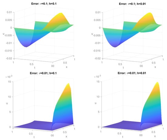
Figure 1. Numerical solution to (47) for $\alpha =0.5$.

Example 4.

Consider the time fractional Black–Scholes Equation (41) for pricing European call options, with a source term $F(x,t)=0$ and initial and boundary conditions:

$${\displaystyle u_0\left(x\right)={(e^x-K)}^{+},u_1\left(t\right)=0,u_2\left(t\right)=e^{B_r}-K{e}^{-rt}.}$$

The European call option premium curves for different values of $\alpha$ are given in Figure 2, for values of the parameters $r=2\%$, $\sigma =30\%$, $B_l=0$, $B_r=200$, $T=1$ (year), and strike price $K=100$. Regarding near-the-money options, lower values of $\alpha$ price them lower and evaluate higher out-of-the-money and in-the-money options, compared to the classical Black–Scholes dynamics.

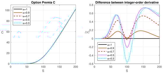
Figure 2. Option premia for various $\alpha$ (left) and the difference between them and the option premium for the integer-order model (right).

The graphs of the call options and put options premiums for $\alpha =0.7$ and all t are given in Figure 3 and Figure 4. To conclude the section with computational simulations, we compare the numerical solutions to (41), using the scheme explained in the paper (7)–(10) and the L1 scheme, as defined, for example, in [55]. We plot the difference as the solution for $\alpha =0.7$, obtained from the L1 scheme, subtracted from the solution, obtained by the ${\mathcal{A}}_n$ scheme (7). The results for $t=T$ and for all t are given on Figure 5.

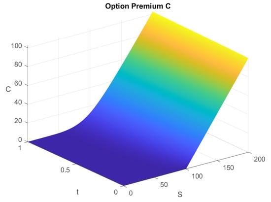
Figure 3. Call options premiums for all t.

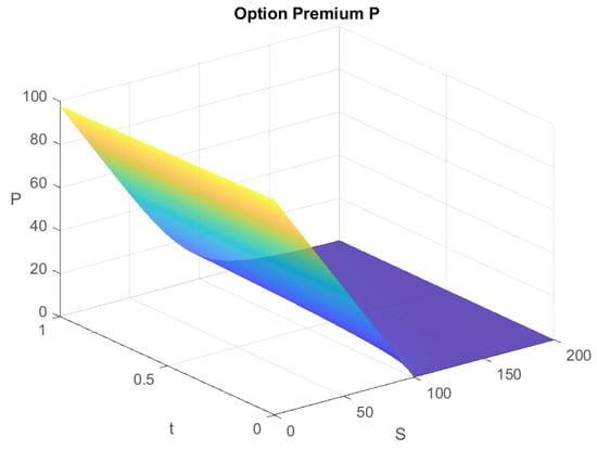
Figure 4. Put options premiums for all t.

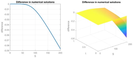
Figure 5. Difference in the numerical solution at $t=T$ (left) and for all t (right).

6. Conclusions

In this paper, we studied the convergence and order of the numerical solutions of ordinary and partial fractional differential equations, which use the approximation (7) of the fractional derivative. The results of the numerical experiments given in the paper illustrated the theoretical results. In future work, we will use the method from [16] for the construction of second-order and high-order approximations of the fractional derivative. We will consider applications of approximations for numerical solutions of linear and nonlinear fractional differential equations and analyze their convergence.

References

- Acay, B.; Bas, E.; Abdeljawad, T. Fractional economic models based on market equilibrium in the frame of different type kernels. Chaos Solit. Fract. 2020, 130, 109438. [Google Scholar] [CrossRef]
- Cardone, A.; Donatelli, M.; Durastante, F.; Garrappa, R.; Mazza, M.; Popolizio, M. Fractional Differential Equations “Modeling, Discretization, and Numerical Solvers”; Springer: Singapore, 2023. [Google Scholar]
- Singh, H.; Kumar, D.; Baleanu, D. Methods of Mathematical Modelling “Fractional Differential Equations”; CRC Press, Taylor & Francis: Boca Raton, FL, USA, 2019. [Google Scholar]
- Shams, M.; Kausar, N.; Samaniego, C.; Agarwal, P.; Ahmed, S.F.; Momani, S. On efficient fractional Caputo-type simultaneous scheme for finding all roots of polynomial equations with biomedical engineering applications. Fractals 2023, 31, 2340075. [Google Scholar] [CrossRef]
- Sun, D.; Liu, J.; Su, X.; Pei, G. Fractional differential equation modeling of the HBV infection with time delay and logistic proliferation. Front. Public Health 2022, 10, 1036901. [Google Scholar] [CrossRef] [PubMed]
- Cai, M.; Li, C. Numerical approaches to fractional integrals and derivatives: A review. Mathematics 2020, 8, 43. [Google Scholar] [CrossRef]
- Jin, B.; Lazarov, R.; Zhou, Z. An analysis of the L1 scheme for the subdiffusion equation with nonsmooth data. IMA J. Numer. Anal. 2016, 36, 197–221. [Google Scholar] [CrossRef]
- Lin, Y.; Xu, C. Finite difference/spectral approximations for the time fractional diffusion equation. J. Comput. Phys. 2007, 225, 1533–1552. [Google Scholar] [CrossRef]
- Mascarenhas, P.V.S.; Moraes, R.M.; Cavalcante, A.L.B. Using a shifted Grünwald–Letnikov scheme for the Caputo derivative to study anomalous solute transport in porous medium. Int. J. Numer. Anal. Methods Geomech. 2019, 43, 1956–1977. [Google Scholar] [CrossRef]
- Scherer, R.; Kalla, S.L.; Tang, Y.; Huang, J. The Grünwald–Letnikov method for fractional differential equations. Comput. Math. Appl. 2011, 62, 902–917. [Google Scholar] [CrossRef]
- Nasir, H.M.; Nafa, K. A new second order approximation for fractional derivatives with applications. SQUJS 2018, 23, 43–55. [Google Scholar]
- Zeng, F.; Li, C.; Liu, F.; Turner, I. Numerical algorithms for time fractional subdiffusion equation with second-order accuracy. SIAM J. Sci. Comput. 2015, 37, A55–A78. [Google Scholar] [CrossRef]
- Dimitrov, Y. A second order approximation for the Caputo fractional derivative. J. Fract. Calc. Appl. 2016, 7, 175–195. [Google Scholar]
- Alikhanov, A.A. A new difference scheme for the time fractional diffusion equation. J. Comput. Phys. 2015, 280, 424–438. [Google Scholar] [CrossRef]
- Gao, G.-H.; Sun, Z.-Z.; Zhang, H.-W. A new fractional numerical differentiation formula to approximate the Caputo fractional derivative and its applications. J. Comput. Phys. 2014, 259, 33–50. [Google Scholar] [CrossRef]
- Apostolov, S.; Dimitrov, Y.; Todorov, V. Constructions of second order approximations of the Caputo fractional derivative. Lect. Notes Comput. Sci. 2022, 13127, 31–39. [Google Scholar]
- Alikhanov, A.A.; Huang, C. A high-order L2 type difference scheme for the time fractional diffusion equation. Appl. Math. Comput. 2021, 411, 1–19. [Google Scholar] [CrossRef]
- Lv, C.; Xu, C. Error analysis of a high order method for time fractional diffusion equations. SIAM J. Sci. Comput. 2016, 38, A2699–A2724. [Google Scholar] [CrossRef]
- Wang, Y.-M.; Ren, L. A high-order L2-compact difference method for Caputo-type time fractional sub-diffusion equations with variable coefficients. Appl. Math. Comput. 2019, 342, 71–93. [Google Scholar] [CrossRef]
- Chen, M.H.; Deng, W.H. Fourth order accurate scheme for the space fractional diffusion equations. SIAM J. Numer. Anal. 2014, 52, 1418–1438. [Google Scholar] [CrossRef]
- Cao, J.; Cai, Z. Numerical analysis of a high-order scheme for nonlinear fractional differential equations with uniform accuracy. Numer. Math. Theory Methods Appl. 2020, 14, 71–112. [Google Scholar] [CrossRef]
- Dehghan, M.; Safarpoor, M.; Abbaszadeh, M. Two high-order numerical algorithms for solving the multi-term time fractional diffusion-wave equations. J. Comput. Appl. Math. 2015, 290, 174–195. [Google Scholar] [CrossRef]
- Li, L.; Zhao, D.; She, M.; Chen, X. On high order numerical schemes for fractional differential equations by block-by-block approach. Appl. Math. Comput. 2022, 425, 127098. [Google Scholar] [CrossRef]
- Lubich, C. Discretized fractional calculus. SIAM J. Math. Anal. 1986, 17, 704–719. [Google Scholar] [CrossRef]
- Ramezani, M.; Mokhtari, R.; Haase, G. Some high order formulae for approximating Caputo fractional derivatives. Appl. Numer. Math. 2020, 153, 300–318. [Google Scholar] [CrossRef]
- Roul, P.; Rohil, V. A novel high-order numerical scheme and its analysis for the two-dimensional time fractional reaction-subdiffusion equation. Numer. Algor. 2022, 90, 1357–1387. [Google Scholar] [CrossRef]
- Wu, R.F.; Ding, H.F.; Li, C.P. Determination of coefficients of high-order schemes for Riemann–Liouville derivative. Sci. World J. 2014, 2014, 402373. [Google Scholar] [CrossRef] [PubMed]
- Navot, I. An extension of the Euler-Maclaurin summation formula to functions with a branch singularity. J. Math. Phys. 1961, 40, 271–276. [Google Scholar] [CrossRef]
- Navot, I. A further extension of the Euler–Maclaurin summation formula. J. Math. Phys. 1962, 41, 155–163. [Google Scholar] [CrossRef]
- Dimitrov, Y. Approximations of the fractional integral and numerical solutions of fractional integral equations. Commun. Appl. Math. Comput. 2021, 3, 545–569. [Google Scholar] [CrossRef]
- Doha, E.H.; Bhrawy, A.H.; Baleanu, D.; Ezz-Eldien, S.S. On shifted Jacobi spectral approximations for solving fractional differential equations. Appl. Math. Comput. 2013, 219, 8042–8056. [Google Scholar] [CrossRef]
- Youssri, Y.H.; Abd-Elhameed, W.M.; Ahmed, H.M. New fractional derivative expression of the shifted third-kind Chebyshev polynomials: Application to a type of nonlinear fractional pantograph differential equations. J. Funct. Spaces 2022, 2022, 3966135. [Google Scholar] [CrossRef]
- Lubich, C. Fractional linear multistep methods for Abel-Volterra integral equations of the second kind. Math. Comp. 1985, 45, 463–469. [Google Scholar] [CrossRef]
- Marasi, H.; Derakhshan, M.H.; Joujehi, A.S.; Kumar, P. Higher-order fractional linear multi-step methods. Phys. Scr. 2023, 98, 024004. [Google Scholar] [CrossRef]
- Abbas, M.; Bibi, A.; Alzaidi, A.S.M.; Nazir, T.; Majeed, A.; Akram, G. Numerical solutions of third-order time fractional differential equations using cubic B-spline functions. Fractal Fract. 2022, 6, 528. [Google Scholar] [CrossRef]
- Duan, J.-S.; Li, M.; Wang, Y.; An, Y.-L. Approximate solution of fractional differential equation by quadratic splines. Fractal Fract. 2022, 6, 369. [Google Scholar] [CrossRef]
- Ray, S.S.; Gupta, A.K. Wavelet Methods for Solving Partial Differential Equations and Fractional Differential Equations; Chapman and Hall/CRC: Boca Raton, FL, USA, 2018. [Google Scholar]
- Ur Rehman, M.; Baleanu, D.; Alzabut, J.; Saeed, I. Green–Haar wavelets method for generalized fractional differential equations. Adv. Differ. Equ. 2020, 515, 2020. [Google Scholar] [CrossRef]
- Dimitrov, Y. Approximations for the Caputo derivative (I). J. Fract. Calc. Appl. 2018, 9, 15–44. [Google Scholar]
- Matsuoka, Y. On the power series coefficients of the Riemann zeta function. Tokyo J. Math. 1989, 12, 49–58. [Google Scholar] [CrossRef]
- Edwards, H.M. Riemann’s Zeta Function; Academic Press: New York, NY, USA, 1974. [Google Scholar]
- Weideman, J.A.C. Numerical integration of periodic functions: A few examples. Am. Math. Mon. 2002, 109, 21–36. [Google Scholar] [CrossRef]
- Anjara, F.; Solofoniaina, J. Solution of general fractional oscillation relaxation equation by Adomian’s method. Gen. Math. Notes 2014, 20, 1–11. [Google Scholar]
- Güulsu, M.; Öztürk, Y.; Anapalı, A. Numerical approach for solving fractional relaxation-oscillation equation. Appl. Math. Model. 2013, 37, 5927–5937. [Google Scholar] [CrossRef]
- Hu, Y.; Luo, Y.; Lu, Z. Analytical solution of the linear fractional differential equation by Adomian decomposition method. J. Comput. Appl. Math. 2008, 215, 220–229. [Google Scholar] [CrossRef]
- Odibat, Z.M.; Momani, S.M. An algorithm for the numerical solution of differential equations of fractional order. J. Appl. Math. Inform. 2008, 26, 15–27. [Google Scholar]
- Podlubny, I. Fractional Differential Equation; Academic Press: Princeton, NJ, USA, 1999. [Google Scholar]
- Ray, S.S.; Bera, R.K. Analytical solution of the Bagley Torvik equation by Adomian decomposition method. Appl. Math. Comput. 2005, 168, 398–410. [Google Scholar] [CrossRef]
- Nuugulu, S.M.; Gideon, F.; Patidar, K.C. A robust numerical solution to a time fractional Black–Scholes equation. Adv. Differ. Equ. 2021, 2021, 123. [Google Scholar] [CrossRef]
- Cen, Z.; Huang, J.; Xu, A.; Le, A. Numerical approximation of a time fractional Black–Scholes equation. Comput. Math. Appl. 2018, 75, 2874–2887. [Google Scholar] [CrossRef]
- Abdi, N.; Aminikhah, H.; Sheikhani, A.H.R. High-order compact finite difference schemes for the time fractional Black–Scholes model governing European options. Chaos Solit. Fract. 2022, 162, 112423. [Google Scholar] [CrossRef]
- Chen, X.; Xu, X.; Zhu, S.-P. Analytically pricing double barrier options based on a time fractional Black–Scholes equation. Comput. Math. Appl. 2015, 69, 1407–1419. [Google Scholar] [CrossRef]
- Wang, X.-T. Scaling and long-range dependence in option pricing I: Pricing European option with transaction costs under the fractional Black–Scholes model. Phys. A Stat. Mech. 2010, 389, 438–444. [Google Scholar] [CrossRef]
- Kumar, S.; Kumar, D.; Singh, J. Numerical computation of fractional Black–Scholes equation arising in financial market. Egypt. J. Basic Appl. Sci. 2014, 1, 177–183. [Google Scholar] [CrossRef]
- Zhang, H.; Liu, F.; Turner, I.; Yang, Q. Numerical solution of the time fractional Black–Scholes model governing European options. Comput. Math. Appl. 2016, 71, 1772–1783. [Google Scholar] [CrossRef]
- Grzegorz Krzyżanowski, G.; Magdziarz, M.; Plociniczak, L. A weighted finite difference method for subdiffusive Black–Scholes model. Comput. Math. Appl. 2020, 80, 653–670. [Google Scholar] [CrossRef]
- Dimitrov, Y.; Vulkov, L. Three-point compact finite difference scheme on non-uniform meshes for the time fractional Black–Scholes equation. AIP Conf. Proc. 2015, 1690, 040022. [Google Scholar]
- Song, L.; Wang, W. Solution of the fractional Black–Scholes option pricing model by finite difference method. Abstr. Appl. Anal. 2013, 2013, 194286. [Google Scholar] [CrossRef]
- Deming, W.; Colcord, C. The minimum in the gamma function. Nature 1935, 135, 917. [Google Scholar] [CrossRef]
- Kolotilina, L.Y. Bounds for the infinity norm of the inverse for certain M- and H-matrices. Linear Algebra Appl. 2009, 430, 692–702. [Google Scholar] [CrossRef]
- Nilson, E.N.; Ahlberg, J.H. Convergence properties of the spline fit. J. SIAM 1963, 11, 95–104. [Google Scholar]
Disclaimer/Publisher’s Note: The statements, opinions and data contained in all publications are solely those of the individual author(s) and contributor(s) and not of MDPI and/or the editor(s). MDPI and/or the editor(s) disclaim responsibility for any injury to people or property resulting from any ideas, methods, instructions or products referred to in the content. |
© 2023 by the authors. Licensee MDPI, Basel, Switzerland. This article is an open access article distributed under the terms and conditions of the Creative Commons Attribution (CC BY) license (https://creativecommons.org/licenses/by/4.0/).