Stochastic Modeling of Three-Species Prey–Predator Model Driven by Lévy Jump with Mixed Holling-II and Beddington–DeAngelis Functional Responses

Abstract

This study examines the dynamics of a stochastic prey–predator model using a functional response function driven by Lévy noise and a mixed Holling-II and Beddington–DeAngelis functional response. The proposed model presents a computational analysis between two prey and one predator population dynamics. First, we show that the suggested model admits a unique positive solution. Second, we prove the extinction of all the studied populations, the extinction of only the predator, and the persistence of all the considered populations under several sufficient conditions. Finally, a special Runge–Kutta method for the stochastic model is illustrated and implemented in order to show the behavior of the two prey and one predator subpopulations.

1. Introduction

Prey–predator dynamics remain a highly fruitful and attractive ecological subject [1,2,3,4]. The basic prey–predator model was proposed by Lotka and Volterra in 1956 [5]; this basic ecological problem was one of the earliest to model competition between prey and predator. One study devoted to the dynamics of fishing illustrated the mathematical and ecological properties of marine fish [6]. Another application of these mathematical tools sought to understand the interaction between wildebeest, zebra, and lion [7] in Kruger National Park in South-Africa. The natural or more realistic growth rate is a logistic suggested by Verhulst [8] for new recruitment of either prey, predators, or both. This logistic growth rate charmed several scientists in various disciplines [9,10,11,12,13,14]. Other studies have been devoted to the type of competition between prey and predators; for example, the basic prey–predator model uses a mass action computational rate [5]. In another study [15], Yavuz and Sene performed a stability analysis for the fractional predator–prey model with harvesting rate. In [16], the authors provided an analysis of the prey–predator model using the Crowley–Martin type functional response. Their main object was to study the stability behavior of the considered population. The Holling-type functional impact on the dynamics of the prey–predator relationship was studied in [17,18]. The starting predator–prey model is based on the assumption that the reaction is between one predator and one prey species. Recently, the authors of [19,20] considered two prey and one predator species under a mixed Holling-II and Beddington–DeAngelis functional response, as follows:

$$\left\{\begin{array}{c}{\displaystyle \frac{d{\mathcal{X}}_1}{dt}}\left(t\right)={\mathcal{X}}_1\left(t\right)\left({\upsilon }_1-{\varrho }_1{\mathcal{X}}_1\left(t\right)-\frac{y\left(t\right)}{{\iota }_1+{\mathcal{X}}_1\left(t\right)}\right),\hfill \\ {\displaystyle \frac{d{\mathcal{X}}_2}{dt}}\left(t\right)={\mathcal{X}}_2\left(t\right)\left({\upsilon }_2-{\varrho }_2{\mathcal{X}}_2\left(t\right)-\frac{y\left(t\right)}{{\iota }_2+{\mathcal{X}}_2\left(t\right)+\beta y\left(t\right)}\right),\hfill \\ {\displaystyle \frac{dy}{dt}}\left(t\right)=y\left(t\right)\left(-d-{\varrho }_{3}y\left(t\right)+\frac{{\vartheta }_1{\mathcal{X}}_1\left(t\right)}{{\iota }_1+{\mathcal{X}}_1\left(t\right)}+\frac{{\vartheta }_2{\mathcal{X}}_2\left(t\right)}{{\iota }_2+{\mathcal{X}}_2\left(t\right)+\beta y\left(t\right)}\right),\hfill \end{array}\right.$$

(1)

where the two prey and one predator populations are presented by ${\mathcal{X}}_1$, ${\mathcal{X}}_2$, and y, respectively. The parameters of (1) and their meanings are provided in

Table 1. The parameters of (1) and their meanings.

Parameters	Description
${\upsilon }_1$	The intrinsic growth rate of prey ${\mathcal{X}}_1$
${\upsilon }_2$	The intrinsic growth rate for ${\mathcal{X}}_2$
${\varrho }_1$	The intra-specific competition for prey ${\mathcal{X}}_1$
${\varrho }_2$	The intra-specific competition for prey ${\mathcal{X}}_2$
${\iota }_1$	The half-saturation due to ${\mathcal{X}}_1$
${\iota }_2$	The half-saturation due to ${\mathcal{X}}_2$
$\beta$	The impact of the predator interference
$\delta$	The death rates of predator
${\varrho }_3$	The rate of intra-species competition for predator
${\vartheta }_1$	The average of the transformation of predator from prey ${\mathcal{X}}_1$
${\vartheta }_2$	The average of the transformation of predator from prey ${\mathcal{X}}_2$
d	The natural mortality of the predator y

.

Deterministic modeling lacks one of the most important properties in prey and predator, that of randomness; for this reason, the stochastic model is preferred in modeling such problems. This is because the stochastic model takes into account the variance aspect, not just the mean, as in the deterministic case. In addition, the stochastic model may offer different predicted results for the same initial data. Certain stochastic prey–predator systems can be established by taking into consideration only the white noise for the studied population [21,22]. Recently, a Brownian random walk perturbation on model (1) was proposed in [20] by studying the persistence and extinction of the prey and predator population. A more basic modification to the modeling technique is to immediately take into account more realistic distributions in order to maintain the model’s straightforward analytic form. This naturally leads to Lévy jumps, a broader class of driving processes [23,24,25,26,27,28,29,30,31,32,33,34,35]. In fact, the dynamical model may encounter abrupt and significant disturbances in predator–prey development due to the intrinsic stochastic features of the related processes [36]. Here, we add the jumps to the model from [20] in response to the results of earlier research. Thus, the model becomes

$$\left\{\begin{array}{cc}{\displaystyle d{\mathcal{X}}_1\left(t\right)=}\hfill & {\mathcal{X}}_1\left(t\right)\left({\upsilon }_1-{\varrho }_1{\mathcal{X}}_1\left(t\right)-\frac{y\left(t\right)}{{\iota }_1+{\mathcal{X}}_1\left(t\right)}\right)dt+{\sigma }_1{\mathcal{X}}_1\left(t\right)d{W}_1\left(t\right)\hfill \\ \hfill & {\displaystyle +{\int }_U{\Xi }_1\left(u\right){\mathcal{X}}_1(t-)\tilde{N}(dt,du),}\hfill \\ {\displaystyle d{\mathcal{X}}_2\left(t\right)=}\hfill & {\mathcal{X}}_2\left(t\right)\left({\upsilon }_2-{\varrho }_2{\mathcal{X}}_2\left(t\right)-\frac{y\left(t\right)}{{\iota }_2+{\mathcal{X}}_2\left(t\right)+\beta y\left(t\right)}\right)dt+{\sigma }_2{\mathcal{X}}_2\left(t\right)d{W}_2\left(t\right)\hfill \\ \hfill & {\displaystyle +{\int }_U{\Xi }_2\left(u\right){\mathcal{X}}_2(t-)\tilde{N}(dt,du),}\hfill \\ {\displaystyle dy\left(t\right)=}\hfill & y\left(t\right)\left(-d-{\varrho }_{3}y\left(t\right)+\frac{{\vartheta }_1{\mathcal{X}}_1\left(t\right)}{{\iota }_1+{\mathcal{X}}_1\left(t\right)}+\frac{{\vartheta }_2{\mathcal{X}}_2\left(t\right)}{{\iota }_2+{\mathcal{X}}_2\left(t\right)+\beta y\left(t\right)}\right)dt+{\sigma }_{3}y\left(t\right)d{W}_3\left(t\right)\hfill \\ \hfill & {\displaystyle +{\int }_U{\Xi }_3\left(u\right)y(t-)\tilde{N}(dt,du).}\hfill \end{array}\right.$$

(2)

where the left limits of ${\mathcal{X}}_1\left(t\right)$, ${\mathcal{X}}_2\left(t\right)$, and $y\left(t\right)$ are denoted by $x(t-)$, $y(t-)$, and $z(t-)$, respectively, the standard Brownian motion $W_i\left(t\right)$ is defined on the space $\left(\Omega ,\mathcal{F},{\left({\mathcal{F}}_t\right)}_{t\ge 0},\mathbb{P}\right)$ as a complete probability, and ${\left({\mathcal{F}}_t\right)}_{t\ge 0}$ is the filtration verifying the usual conditions. We define the finite stationary compensator $\nu$ on U as the measurable subset of the non-negative half-line; then, $N(dt,du)$ is the Poisson counting $\nu \left(du\right)dt$, ${\sigma }_i$ is the intensity of $W_i\left(t\right)$, and the jumping intensities are represented by $q_i\left(u\right)$ for $i=1,2,3$.

The remaining parts of this study are organized as follows. In Section 2, we provide several properties of the solution of the model (2). The stochastic extinction of both the prey and the predator is established in Section 3. In Section 4, we prove the persistence of the prey and the extinction of the predator. The stochastic persistence of both the predator and prey is illustrated in Section 5. Finally, Section 6 of this paper is devoted to numerical simulations that validate our theoretical findings.

2. The Well-Posedness of the Solution

The following theorem ensures the well-posedness of the solution of the model (2).

Theorem 1. 

For all initial conditions that are positive, model (2) admits a unique positive global solution a.s.

Proof. 

Using the local Lipschitz of the diffusion and drift, for all initial positive data the problem (2) admits a local unique solution $\left({\mathcal{X}}_1\left(t\right),{\mathcal{X}}_2\left(t\right),y\left(t\right)\right)$ for $t\in [0,T^e)$, with $T^e$ representing the time of explosion.

Proving the existence globality of the solution amounts to showing that $T^e=\infty$ a.s. For a given a large number $n_0^{\prime }>0$, for any integer $n^{\prime }\ge n_0^{\prime }$ the stopping time is defined as

$$T^{n^{\prime }}=inf\{t\in [0,T^e)/{\mathcal{X}}_1\left(t\right)\notin ({\displaystyle \frac{1}{n^{\prime }}},n^{\prime })\mathrm{or}{\mathcal{X}}_2\left(t\right)\notin ({\displaystyle \frac{1}{n^{\prime }}},n^{\prime })\mathrm{or}y\left(t\right)\notin ({\displaystyle \frac{1}{n^{\prime }}},n^{\prime })\},$$

and when $n^{\prime }\uparrow \infty$, the number $T^{n^{\prime }}$ increases. Using $T^{\infty }={lim}_{n^{\prime }\to \infty }{T}^{n^{\prime }}$, with $T^{\infty }\le T^e$ a.s., it is sufficient to prove that $T^{\infty }=\infty$, which is signified $T^e=\infty$, and $\left({\mathcal{X}}_1\left(t\right),{\mathcal{X}}_2\left(t\right),y\left(t\right)\right)\in {\mathbb{R}}_{+}^3$ a.s. Suppose the contrary, i.e., $T^{\infty }<\infty$ a.s. This means that there exists some $T>0$ and $0<ϵ<1$ such that $\mathbb{P}(T^{\infty }\le T)\ge ϵ$.

Considering the functional

$$V\left({\mathcal{X}}_1\left(t\right),{\mathcal{X}}_2\left(t\right),y\left(t\right)\right)=\left({\mathcal{X}}_1-1-log\left({\mathcal{X}}_1\right)\right)+\left({\mathcal{X}}_2-1-log\left({\mathcal{X}}_2\right)\right)+\left(y-1-log\left(y\right)\right),$$

from Itô’s formula [37], we obtain

$$\begin{array}{cc}\hfill dV\left({\mathcal{X}}_1,{\mathcal{X}}_2,y\right)=& LVdt+{\sigma }_1({\mathcal{X}}_1-1)d{W}_1+{\sigma }_2({\mathcal{X}}_2-1)d{W}_2+{\sigma }_3(y-1)d{W}_3\hfill \\ \hfill & +{\int }_U\left[{\Xi }_1\left(u\right){\mathcal{X}}_1-log\left(1+{\Xi }_1\left(u\right){\mathcal{X}}_1\right)\right]\hfill \\ \hfill & +{\int }_U\left[{\Xi }_2\left(u\right){\mathcal{X}}_2-log\left(1+{\Xi }_2\left(u\right){\mathcal{X}}_2\right)\right]\hfill \\ \hfill & +{\int }_U\left[{\Xi }_3\left(u\right)y-log\left(1+{\Xi }_3\left(u\right)y\right)\right],\hfill \end{array}$$

(3)

with

$$\begin{array}{cc}\hfill LV=& \left(1-{\displaystyle \frac{1}{{\mathcal{X}}_1}}\right)\left({\mathcal{X}}_1\left(t\right)\left({\upsilon }_1-{\varrho }_1{\mathcal{X}}_1-{\displaystyle \frac{y}{{\iota }_1+{\mathcal{X}}_1}}\right)\right)+{\displaystyle \frac{{\sigma }_1^2}{2}}\hfill \\ \hfill & +\left(1-{\displaystyle \frac{1}{{\mathcal{X}}_2}}\right)\left({\mathcal{X}}_2\left(t\right)\left({\upsilon }_2-{\varrho }_2{\mathcal{X}}_2-{\displaystyle \frac{y}{{\iota }_2+{\mathcal{X}}_2+\beta y}}\right)\right)+{\displaystyle \frac{{\sigma }_2^2}{2}}\hfill \\ \hfill & +\left(1-{\displaystyle \frac{1}{y}}\right)\left(y\left(-d-{\varrho }_{3}y+{\displaystyle \frac{{\vartheta }_1{\mathcal{X}}_1}{{\iota }_1+{\mathcal{X}}_1}}+{\displaystyle \frac{{\vartheta }_2{\mathcal{X}}_2}{{\iota }_2+{\mathcal{X}}_2+\beta y}}\right)\right)+{\displaystyle \frac{\rho {\sigma }_3^2}{2}}\hfill \\ \hfill & +{\int }_U\left[{\Xi }_1\left(u\right)-log\left(1+{\Xi }_1\left(u\right)\right)\right]\nu \left(du\right)\hfill \\ \hfill & +{\int }_U\left[{\Xi }_2\left(u\right)-log\left(1+{\Xi }_2\left(u\right)\right)\right]\nu \left(du\right)\hfill \\ \hfill & +{\int }_U\left[{\Xi }_3\left(u\right)-log\left(1+{\Xi }_3\left(u\right)\right)\right]\nu \left(du\right),\hfill \end{array}$$

then,

$$\begin{array}{cc}\hfill LV\le & {\upsilon }_1{\mathcal{X}}_1-{\varrho }_1{\mathcal{X}}_1^2+{\varrho }_1{\mathcal{X}}_1+{\displaystyle \frac{{\sigma }_1^2}{2}}\hfill \\ \hfill & +{\upsilon }_2{\mathcal{X}}_2-{\varrho }_1{\mathcal{X}}_2^2+{\varrho }_2{\mathcal{X}}_2+{\displaystyle \frac{{\sigma }_2^2}{2}}\hfill \\ \hfill & +d+({\vartheta }_1+{\vartheta }_2)y-{\varrho }_3{y}^2+{\displaystyle \frac{{\sigma }_2^3}{2}}+M,\hfill \\ \hfill LV\le & ({\upsilon }_1+{\varrho }_1){\mathcal{X}}_1-{\varrho }_1{\mathcal{X}}_1^2+{\displaystyle \frac{{\sigma }_1^2}{2}}+({\upsilon }_2+{\varrho }_2){\mathcal{X}}_2-{\varrho }_2{\mathcal{X}}_2^2+{\displaystyle \frac{{\sigma }_2^2}{2}}\hfill \\ \hfill & +d+({\vartheta }_1+{\vartheta }_2)y-{\varrho }_3{y}^2+{\displaystyle \frac{{\sigma }_3^2}{2}}+3C^{\prime },\hfill \\ \hfill LV\le & {\displaystyle \frac{{({\upsilon }_1+{\varrho }_1)}^2}{4{\varrho }_1}}+{\displaystyle \frac{{({\upsilon }_2+{\varrho }_2)}^2}{4{\varrho }_2}}+d+{\displaystyle \frac{{({\vartheta }_1+{\vartheta }_2)}^2}{4{\varrho }_3}}+{\displaystyle \frac{{\sigma }_1^2}{2}}+{\displaystyle \frac{{\sigma }_2^2}{2}}+{\displaystyle \frac{{\sigma }_3^2}{2}}+M,\hfill \\ \hfill LV\le & M^{\prime },\hfill \end{array}$$

with

$$\begin{array}{cc}\hfill M=& 3max\{{\int }_U\left[{\Xi }_1\left(u\right)-log\left(1+{\Xi }_1\left(u\right)\right)\right]\nu \left(du\right),{\int }_U\left[{\Xi }_2\left(u\right)-log\left(1+{\Xi }_2\left(u\right)\right)\right]\nu \left(du\right),\hfill \\ \hfill & {\int }_U\left[{\Xi }_3\left(u\right)-log\left(1+{\Xi }_3\left(u\right)\right)\right]\nu \left(du\right)\}.\hfill \end{array}$$

$$\begin{array}{cc}\hfill M& ={\displaystyle \frac{{({\upsilon }_1+{\varrho }_1)}^2}{4{\varrho }_1}}+{\displaystyle \frac{{({\upsilon }_2+{\varrho }_2)}^2}{4{\varrho }_2}}+d+{\displaystyle \frac{{({\vartheta }_1+{\vartheta }_2)}^2}{4{\varrho }_3}}+{\displaystyle \frac{{\sigma }_1^2}{2}}+{\displaystyle \frac{{\sigma }_2^2}{2}}+{\displaystyle \frac{{\sigma }_3^2}{2}}+M^{\prime }.\hfill \end{array}$$

Integrating Equation (3) between 0 and $T^{n^{\prime }}\wedge T,$ we obtain

$$\begin{array}{c}\hfill 0\le \mathbb{E}\left(V\left({\mathcal{X}}_1(T^{n^{\prime }}\wedge T),{\mathcal{X}}_2(T^{n^{\prime }}\wedge T),y(T^{n^{\prime }}\wedge T)\right)\right)\\ \hfill \le V\left({\mathcal{X}}_1\left(0\right),{\mathcal{X}}_2\left(0\right),y\left(0\right)\right)+M^{\prime }T.\end{array}$$

Thus, if $n^{\prime }\to \infty$, then

$$\infty >V\left({\mathcal{X}}_1\left(0\right),{\mathcal{X}}_2\left(0\right),y\left(0\right)\right)+M^{\prime }CT=\infty ,$$

which is in contradiction with the previous supposition. Thus, $T^{\infty }=\infty$ and the solution $({\mathcal{X}}_1\left(t\right),{\mathcal{X}}_2\left(t\right),y\left(t\right))$ is unique and global a.s. □

3. Stochastic Extinction

Now, we prove the extinction of the three subpopulations a.s. First, we define

$$\begin{array}{cc}\hfill m_1& ={\upsilon }_1+{\int }_{U}log\left(1+{\Xi }_1\left(u\right)\right)-{\Xi }_1\left(u\right)\nu \left(du\right)-{\displaystyle \frac{{\sigma }_1^2}{2}},\hfill \\ \hfill m_2& ={\upsilon }_2+{\int }_{U}log\left(1+{\Xi }_2\left(u\right)\right)-{\Xi }_2\left(u\right)\nu \left(du\right)-{\displaystyle \frac{{\sigma }_2^2}{2}},\hfill \\ \hfill m_3& ={\displaystyle \frac{{\vartheta }_1}{{\varrho }_1}}\left({\upsilon }_1+{\int }_{U}log\left(1+{\Xi }_1\left(u\right)\right)-{\Xi }_1\left(u\right)\nu \left(du\right)-{\displaystyle \frac{{\sigma }_1^2}{2}}\right)\hfill \\ \hfill & +{\displaystyle \frac{{\vartheta }_2}{{\varrho }_2}}\left({\upsilon }_2+{\int }_{U}log\left(1+{\Xi }_2\left(u\right)\right)-{\Xi }_2\left(u\right)\nu \left(du\right)-{\displaystyle \frac{{\sigma }_2^2}{2}}\right)-d\hfill \\ \hfill & +{\int }_{U}log\left(1+{\Xi }_3\left(u\right)\right)-{\Xi }_3\left(u\right)\nu \left(du\right)-{\displaystyle \frac{{\sigma }_3^2}{2}}.\hfill \end{array}$$

Theorem 2. 

If $max\{m_1,m_2,m_3\}<0,$ then for any initial positive condition we have

$$\begin{array}{cc}\hfill & \underset{t\to +\infty }{lim}<{\mathcal{X}}_1{>}_t =0,\hfill \\ \hfill & \underset{t\to +\infty }{lim}<{\mathcal{X}}_2{>}_t =0,\hfill \\ \hfill & \underset{t\to +\infty }{lim}<y{>}_t =0.\hfill \end{array}$$

Proof. 

Considering

$$\mathcal{F}\left({\mathcal{X}}_1\right)=log\left({\mathcal{X}}_1\left(t\right)\right),$$

from Itô’s formula we have

$$\begin{array}{cc}\hfill d\mathcal{F}=& L\mathcal{F}dt+{\sigma }_{1}d{W}_1\left(t\right)+{\int }_{U}log\left(1+{\Xi }_1\left(u\right)\right)\tilde{N}(dt,du),\hfill \end{array}$$

(4)

with

$$\begin{array}{cc}\hfill L\mathcal{F}=& {\upsilon }_1-{\varrho }_1{\mathcal{X}}_1-\frac{y}{{\iota }_1+{\mathcal{X}}_1}-{\displaystyle \frac{{\sigma }_1^2}{2}}+{\int }_{U}log\left(1+{\Xi }_1\left(u\right)\right)-{\Xi }_1\left(u\right)\nu \left(du\right),\hfill \end{array}$$

then,

$$L\mathcal{F}\le {\upsilon }_1-{\varrho }_1{\mathcal{X}}_1-{\displaystyle \frac{{\sigma }_1^2}{2}}+{\int }_{U}log\left(1+{\Xi }_1\left(u\right)\right)-{\Xi }_1\left(u\right)\nu \left(du\right),$$

and,

$$\begin{array}{cc}\hfill {\displaystyle \frac{log\left({\mathcal{X}}_1\left(t\right)\right)-log\left({\mathcal{X}}_1\left(0\right)\right)}{t}}& \le {\upsilon }_1-{\displaystyle \frac{{\sigma }_1^2}{2}}+{\int }_{U}log\left(1+{\Xi }_1\left(u\right)\right)-{\Xi }_1\left(u\right)\nu \left(du\right)\hfill \\ \hfill & -{\varrho }_1<{\mathcal{X}}_1{>}_t+{\int }_0^t{\displaystyle \frac{{\sigma }_{1}d{W}_1\left(s\right)}{t}}ds\hfill \\ \hfill & +{\displaystyle \frac{1}{t}}{\int }_0^t{\int }_{U}log\left(1+{\Xi }_1\left(u\right)\right)\tilde{N}(ds,du)ds,\hfill \end{array}$$

therefore,

$$\begin{array}{cc}\hfill <{\mathcal{X}}_1{>}_t \le & {\displaystyle \frac{1}{{\varrho }_1}}\left({\upsilon }_1+{\int }_{U}log\left(1+{\Xi }_1\left(u\right)\right)-{\Xi }_1\left(u\right)\nu \left(du\right)-{\displaystyle \frac{{\sigma }_1^2}{2}}\right)\hfill \\ \hfill & +{\displaystyle \frac{1}{{\varrho }_1}}\left({\int }_0^t{\displaystyle \frac{{\sigma }_{1}d{W}_1\left(s\right)}{t}}ds+{\displaystyle \frac{1}{t}}{\int }_0^t{\int }_{U}log\left(1+{\Xi }_1\left(u\right)\right)\tilde{N}(ds,du)ds\right)\hfill \\ \hfill & -{\displaystyle \frac{1}{{\varrho }_1}}{\displaystyle \frac{\left(log\left({\mathcal{X}}_1\left(t\right)\right)-log\left({\mathcal{X}}_1\left(0\right)\right)\right)}{t}}.\hfill \end{array}$$

Let us now take

$$M_t={\int }_0^t{\sigma }_{1}d{W}_1\left(s\right),$$

then,

$$\begin{array}{c}\hfill \underset{t\to +\infty }{lim\; sup}{\displaystyle \frac{<M_t,M_t>}{t}}=\underset{t\to +\infty }{lim\; sup}{\displaystyle \frac{{\sigma }_1^2}{t}}<\infty .\end{array}$$

Using Martingale’s theorem (the strong law of large numbers), we obtain

$$\begin{array}{c}\hfill \underset{t\to +\infty }{lim\; sup}{\displaystyle \frac{M_t}{t}}=0.\end{array}$$

Thus,

$$\begin{array}{cc}\underset{t\to +\infty }{lim}<{\mathcal{X}}_1{>}_t \le & {\displaystyle \frac{1}{{\varrho }_1}}\left({\upsilon }_1+{\int }_{U}log\left(1+{\Xi }_1\left(u\right)\right)-{\Xi }_1\left(u\right)\nu \left(du\right)-{\displaystyle \frac{{\sigma }_1^2}{2}}\right).\hfill \end{array}$$

Following the same technique, we obtain

$$\begin{array}{cc}\underset{t\to +\infty }{lim\; inf}<{\mathcal{X}}_2{>}_t \le & {\displaystyle \frac{1}{{\varrho }_2}}\left({\varrho }_2+{\int }_{U}log\left(1+{\Xi }_2\left(u\right)\right)-{\Xi }_2\left(u\right)\nu \left(du\right)-{\displaystyle \frac{{\sigma }_2^2}{2}}\right).\hfill \end{array}$$

We next consider

$$\mathcal{V}\left(t\right)=log\left(y\right).$$

Itô’s formula implies that

$$\begin{array}{cc}\hfill d\mathcal{V}=& L\mathcal{V}dt+{\sigma }_{3}d{W}_3\left(t\right)+{\int }_{U}log\left(1+{\Xi }_3\left(u\right)\right)\tilde{N}(dt,du),\hfill \end{array}$$

(5)

with

$$\begin{array}{cc}\hfill L\mathcal{V}=& -d-{\varrho }_{3}z+\frac{{\vartheta }_1{\mathcal{X}}_1}{{\iota }_1+{\mathcal{X}}_1}+{\displaystyle \frac{{\vartheta }_2{\mathcal{X}}_2}{{\iota }_2+{\mathcal{X}}_2+\beta y}}-{\displaystyle \frac{{\sigma }_3^2}{2}}+{\int }_{U}log\left(1+{\Xi }_3\left(u\right)\right)-{\Xi }_3\left(u\right)\nu \left(du\right)\hfill \\ \hfill \le & -d-{\varrho }_{3}y+{\vartheta }_1{\mathcal{X}}_1+{\vartheta }_2{\mathcal{X}}_2+{\int }_{U}log\left(1+{\Xi }_3\left(u\right)\right)-{\Xi }_3\left(u\right)\nu \left(du\right)-{\displaystyle \frac{{\sigma }_3^2}{2}},\hfill \end{array}$$

then,

$$\begin{array}{cc}\hfill {\displaystyle \frac{\mathcal{V}\left(t\right)-\mathcal{V}\left(0\right)}{t}}\le & {\vartheta }_1<{\mathcal{X}}_1>+{\vartheta }_2<{\mathcal{X}}_2>-d-{\varrho }_3<y{>}_t+{\int }_{U}log\left(1+{\Xi }_3\left(u\right)\right)-{\Xi }_3\left(u\right)\nu \left(du\right)\hfill \\ & -{\displaystyle \frac{{\sigma }_3^2}{2}}+{\displaystyle \frac{1}{t}}{\int }_0^t\left({\sigma }_{3}d{W}_3\left(t\right)+{\int }_{U}log\left(1+{\Xi }_3\left(u\right)\right)\tilde{N}(dt,du)\right),\hfill \end{array}$$

then,

$$\begin{array}{cc}\hfill <y{>}_t \le & {\displaystyle \frac{1}{{\varrho }_3}}\left({\vartheta }_1<{\mathcal{X}}_1>+{\vartheta }_2<{\mathcal{X}}_2>-d-{\displaystyle \frac{{\sigma }_3^2}{2}}+{\int }_{U}log\left(1+{\Xi }_3\left(u\right)\right)-{\Xi }_3\left(u\right)\nu \left(du\right)\right)\hfill \\ \hfill & -{\displaystyle \frac{1}{{\varrho }_3}}{\displaystyle \frac{\mathcal{V}\left(t\right)-\mathcal{V}\left(0\right)}{t}}+{\displaystyle \frac{1}{{\alpha }_3}}{\displaystyle \frac{1}{t}}{\int }_0^t\left({\sigma }_{3}d{W}_3\left(t\right)+{\int }_{U}log\left(1+{\Xi }_3\left(u\right)\right)\tilde{N}(dt,du)\right).\hfill \end{array}$$

Similar to $<{\mathcal{X}}_1{>}_t$, we have

$$\begin{array}{cc}\hfill \underset{t\to +\infty }{lim}<y{>}_t \le & {\displaystyle \frac{1}{{\varrho }_3}}({\displaystyle \frac{{\vartheta }_1}{{\varrho }_1}}\left({\upsilon }_1+{\int }_{U}log\left(1+{\Xi }_1\left(u\right)\right)-{\Xi }_1\left(u\right)\nu \left(du\right)-{\displaystyle \frac{{\sigma }_1^2}{2}}\right)\hfill \\ \hfill & +{\displaystyle \frac{{\vartheta }_2}{{\varrho }_2}}\left({\upsilon }_2+{\int }_{U}log\left(1+{\Xi }_2\left(u\right)\right)-{\Xi }_2\left(u\right)\nu \left(du\right)-{\displaystyle \frac{{\sigma }_2^2}{2}}\right)\hfill \\ \hfill & +{\int }_{U}log\left(1+{\Xi }_3\left(u\right)\right)-{\Xi }_3\left(u\right)\nu \left(du\right)-d-{\displaystyle \frac{{\sigma }_3^2}{2}}).\hfill \end{array}$$

□

4. Stochastic Extinction of Predator

In order to prove the extinction of the predator, we need to define

$$\begin{array}{cc}\hfill m_1^{\prime }& ={\displaystyle \frac{m_1}{2{\varrho }_1-{\upsilon }_1}},\hfill \\ \hfill m_2^{\prime }& ={\displaystyle \frac{m_2}{2{\varrho }_2-{\upsilon }_2}},\hfill \\ \hfill m_4& ={\vartheta }_1+{\vartheta }_2-d+{\int }_{U}log\left(1+{\Xi }_3\left(u\right)\right)-{\Xi }_3\left(u\right)\nu \left(du\right)-{\displaystyle \frac{{\sigma }_3^2}{2}}.\hfill \end{array}$$

Theorem 3. 

Suppose that $m_4\le 0$ and $min\{m_1^{\prime },m_2^{\prime }\}>0$; then,

$$\underset{t\to \infty }{lim}<y{>}_t =0,$$

and

$$\begin{array}{cc}\underset{t\to \infty }{lim\; inf}<{\mathcal{X}}_1{>}_t \ge & m_1^{\prime }a.s.\hfill \\ \hfill \underset{t\to \infty }{lim\; inf}<{\mathcal{X}}_2{>}_t \ge & m_2^{\prime }a.s.\hfill \end{array}$$

Proof. 

The first Equation of (2) implies that

$$\begin{array}{cc}\hfill {\displaystyle \frac{{\mathcal{X}}_1\left(t\right)-{\mathcal{X}}_1\left(0\right)}{t}}=& {\displaystyle \frac{1}{t}}{\int }_0^t\left({\mathcal{X}}_1\left(s\right)\left({\upsilon }_1-{\varrho }_1{\mathcal{X}}_1\left(s\right)\right)-{\displaystyle \frac{y\left(s\right)}{{\iota }_1+{\mathcal{X}}_1\left(s\right)}}\right)ds+{\sigma }_{1}x\left(s\right)d{W}_1\left(s\right)\hfill \\ \hfill & +{\displaystyle \frac{1}{t}}{\int }_0^t\left({\displaystyle {\int }_U{\Xi }_1\left(u\right){\mathcal{X}}_1(s-)\tilde{N}(ds,du)}\right)ds.\hfill \end{array}$$

Let us consider the following:

$$\mathcal{F}\left({\mathcal{X}}_1\right)=log\left({\mathcal{X}}_1\left(t\right)\right),$$

from It’ô’s formula, we have

$$\begin{array}{cc}\hfill d\mathcal{F}=& {\upsilon }_1-{\varrho }_1{\mathcal{X}}_1-{\displaystyle \frac{{\sigma }_1^2}{2}}+{\int }_{U}log\left(1+{\Xi }_1\left(u\right)\right)-{\Xi }_1\left(u\right)\nu \left(du\right)\hfill \\ \hfill & -{\displaystyle \frac{y}{{\iota }_1+{\mathcal{X}}_1}}dt+{\sigma }_{1}d{W}_1\left(t\right)+{\int }_{U}log\left(1+{\Xi }_1\left(u\right)\right)\tilde{N}(dt,du),\hfill \end{array}$$

then,

$$\begin{array}{cc}\hfill {\displaystyle \frac{{\mathcal{X}}_1\left(t\right)-{\mathcal{X}}_1\left(0\right)}{t}}+{\displaystyle \frac{\mathcal{F}\left(t\right)-\mathcal{F}\left(0\right)}{t}}\ge & {\upsilon }_1<{\mathcal{X}}_1{>}_t-2{\varrho }_1<{\mathcal{X}}_1{>}_t-{\displaystyle \frac{1}{t}}{\int }_0^t{\displaystyle \frac{({\mathcal{X}}_1+1)y}{{\iota }_1+{\mathcal{X}}_1}}ds\hfill \\ \hfill & +{\upsilon }_1-{\displaystyle \frac{{\sigma }_1^2}{2}}+{\int }_0^t{\int }_{U}log\left(1+{\Xi }_1\left(u\right)\right)-{\Xi }_1\left(u\right)\nu \left(du\right)ds\hfill \\ \hfill & +{\displaystyle \frac{1}{t}}{\int }_0^t{\sigma }_1(1+{\mathcal{X}}_1\left(s\right))d{W}_1\left(s\right)\hfill \\ \hfill & +{\displaystyle \frac{1}{t}}{\int }_0^t\left({\displaystyle {\int }_{U}log\left(1+{\Xi }_1\left(u\right)\right)+{\Xi }_1\left(u\right){\mathcal{X}}_1(s-)\tilde{N}(ds,du)}\right)ds\hfill \end{array}$$

and we know that

$$\underset{t\to +\infty }{lim}{\displaystyle \frac{1}{t}}{\int }_0^t{\displaystyle \frac{({\mathcal{X}}_1+1)y}{{\iota }_1+{\mathcal{X}}_1}}ds\le \underset{t\to +\infty }{lim}{\displaystyle \frac{1}{t}}{\left({\int }_0^t{\left({\displaystyle \frac{({\mathcal{X}}_1+1)}{{\iota }_1+{\mathcal{X}}_1}}\right)}^{2}ds\right)}^{1/2}\times {\left({\int }_0^t{y}^{2}ds\right)}^{1/2}=0.$$

Thus,

$$\underset{t\to +\infty }{lim\; inf}<{\mathcal{X}}_1{>}_t \ge {\displaystyle \frac{{\upsilon }_1+{\int }_{U}log\left(1+{\Xi }_1\left(u\right)\right)-{\Xi }_1\left(u\right)\nu \left(du\right)-\frac{{\sigma }_1^2}{2}}{2{\varrho }_1-{\upsilon }_1}}.$$

Using the same technique, we can show that

$$\underset{t\to +\infty }{lim\; inf}<{\mathcal{X}}_2{>}_t \ge {\displaystyle \frac{{\upsilon }_2+{\int }_{U}log\left(1+{\Xi }_2\left(u\right)\right)-{\Xi }_2\left(u\right)\nu \left(du\right)-\frac{{\sigma }_2^2}{2}}{2{\varrho }_2-{\upsilon }_2}}.$$

Let us now take

$$\mathcal{V}\left(t\right)=log\left(y\right),$$

from Itô’s formula, we have

$$\begin{array}{cc}\hfill d\mathcal{V}=& L\mathcal{V}dt+{\sigma }_{3}d{W}_3\left(t\right)+{\int }_{U}log\left(1+{\Xi }_3\left(u\right)\right)\tilde{N}(dt,du),\hfill \end{array}$$

(6)

with

$$\begin{array}{cc}\hfill L\mathcal{V}=& -d-{\varrho }_{3}y+{\displaystyle \frac{{\vartheta }_1{\mathcal{X}}_1}{{\iota }_1+{\mathcal{X}}_1}}+{\displaystyle \frac{{\vartheta }_2{\mathcal{X}}_2}{{\iota }_2+{\mathcal{X}}_2+\beta y}}-{\displaystyle \frac{{\sigma }_3^2}{2}}+{\int }_{U}log\left(1+{\Xi }_3\left(u\right)\right)-{\Xi }_3\left(u\right)\nu \left(du\right)\hfill \\ \hfill \le & -d-{\varrho }_{3}y+{\upsilon }_1+{\upsilon }_2-{\displaystyle \frac{{\sigma }_3^2}{2}},\hfill \end{array}$$

therefore,

$$\begin{array}{cc}\hfill {\displaystyle \frac{\mathcal{V}\left(t\right)-\mathcal{V}\left(0\right)}{t}}\le & {\vartheta }_1+{\vartheta }_2-d-{\varrho }_3<y{>}_t+{\int }_{U}log\left(1+{\Xi }_3\left(u\right)\right)-{\Xi }_3\left(u\right)\nu \left(du\right)-{\displaystyle \frac{{\sigma }_3^2}{2}}\hfill \\ \hfill & +{\displaystyle \frac{1}{t}}{\int }_0^t\left({\sigma }_{3}d{W}_3\left(t\right)+{\int }_{U}log\left(1+{\Xi }_3\left(u\right)\right)\tilde{N}(dt,du)\right),\hfill \end{array}$$

then,

$$\begin{array}{cc}\hfill <y{>}_t \le & {\displaystyle \frac{1}{{\varrho }_3}}\left({\vartheta }_1+{\vartheta }_2-d+{\int }_{U}log\left(1+{\Xi }_3\left(u\right)\right)-{\Xi }_3\left(u\right)\nu \left(du\right)-{\displaystyle \frac{{\sigma }_3^2}{2}}\right)-{\displaystyle \frac{1}{{\varrho }_3}}{\displaystyle \frac{\mathcal{V}\left(t\right)-\mathcal{V}\left(0\right)}{t}}\hfill \\ \hfill & +{\displaystyle \frac{1}{{\varrho }_3}}{\displaystyle \frac{1}{t}}{\int }_0^t\left({\sigma }_{3}d{W}_3\left(t\right)+{\int }_{U}log\left(1+{\Xi }_3\left(u\right)\right)\tilde{N}(dt,du)\right),\hfill \end{array}$$

and

$$\begin{array}{cc}\hfill \underset{t\to +\infty }{lim}<y{>}_t \le & {\displaystyle \frac{1}{{\varrho }_3}}\left({\vartheta }_1+{\vartheta }_2-d+{\int }_{U}log\left(1+{\Xi }_3\left(u\right)\right)-{\Xi }_3\left(u\right)\nu \left(du\right)-{\displaystyle \frac{{\sigma }_3^2}{2}}\right).\hfill \end{array}$$

□

5. Stochastic Persistence

In this section, we show that all three subpopulations persist.

Theorem 4. 

For $m_1^{\prime }>0$, $m_2^{\prime }>0$, and

$$\begin{array}{cc}\hfill & {\displaystyle \frac{1}{{\varrho }_3}}({\displaystyle \frac{{\upsilon }_1{\vartheta }_1+{\vartheta }_1{\int }_{U}log\left(1+{\Xi }_1\left(u\right)\right)-{\Xi }_1\left(u\right)\nu \left(du\right)-\frac{{\vartheta }_1{\sigma }_1^2}{2}}{({\iota }_1+{\displaystyle \frac{{\upsilon }_1}{2{\varrho }_1}})({\upsilon }_1-2{\varrho }_1)}}\hfill \\ \hfill & +{\displaystyle \frac{{\upsilon }_2{\vartheta }_2+{\vartheta }_2{\int }_{U}log\left(1+{\Xi }_2\left(u\right)\right)-{\Xi }_2\left(u\right)\nu \left(du\right)-\frac{{\vartheta }_2{\sigma }_2^2}{2}}{({\iota }_2+{\displaystyle \frac{{\upsilon }_2}{2{\varrho }_2}}+\beta {\displaystyle \frac{{\upsilon }_2}{2{\varrho }_2}})({\upsilon }_2-2{\varrho }_2)}}\hfill \\ \hfill & -d+{\int }_{U}log\left(1+{\Xi }_3\left(u\right)\right)-{\Xi }_3\left(u\right)\nu \left(du\right)-{\displaystyle \frac{{\sigma }_3^2}{2}})>0,\hfill \end{array}$$

which means that all of the subpopulations persist in the mean. In addition,

$$\begin{array}{cc}\hfill \underset{t\to +\infty }{lim\; inf}<{\mathcal{X}}_1{>}_t \ge & {\displaystyle \frac{{\upsilon }_1+{\int }_{U}log\left(1+{\Xi }_1\left(u\right)\right)-{\Xi }_1\left(u\right)\nu \left(du\right)-\frac{{\sigma }_1^2}{2}}{2{\varrho }_1-{\upsilon }_1}}a.s.\hfill \\ \hfill \underset{t\to +\infty }{lim\; inf}<{\mathcal{X}}_2{>}_t \ge & {\displaystyle \frac{{\upsilon }_2+{\int }_{U}log\left(1+{\Xi }_2\left(u\right)\right)-{\Xi }_2\left(u\right)\nu \left(du\right)-\frac{{\sigma }_2^2}{2}}{2{\varrho }_2-{\upsilon }_2}}a.s.\hfill \\ \hfill \underset{t\to +\infty }{lim\; inf}<y{>}_t \ge & {\displaystyle \frac{1}{{\varrho }_3}}({\displaystyle \frac{{\upsilon }_1{\vartheta }_1+{\vartheta }_1{\int }_{U}log\left(1+{\Xi }_1\left(u\right)\right)-{\Xi }_1\left(u\right)\nu \left(du\right)-\frac{{\vartheta }_1{\sigma }_1^2}{2}}{({\iota }_1+{\displaystyle \frac{{\upsilon }_1}{2{\varrho }_1}})({\upsilon }_1-2{\varrho }_1)}}\hfill \\ \hfill & +{\displaystyle \frac{{\upsilon }_2{\vartheta }_2+{\vartheta }_2{\int }_{U}log\left(1+{\Xi }_2\left(u\right)\right)-{\Xi }_2\left(u\right)\nu \left(du\right)-\frac{{\vartheta }_2{\sigma }_2^2}{2}}{({\iota }_2+{\displaystyle \frac{{\upsilon }_2}{2{\varrho }_2}}+\beta {\displaystyle \frac{{\upsilon }_2}{2{\varrho }_2}})({\upsilon }_2-2{\varrho }_2)}}\hfill \\ \hfill & -d+{\int }_{U}log\left(1+{\Xi }_3\left(u\right)\right)-{\Xi }_3\left(u\right)\nu \left(du\right)-{\displaystyle \frac{{\sigma }_3^2}{2}})a.s.\hfill \end{array}$$

Proof. 

The first Equation of (2) implies that

$$\begin{array}{cc}\hfill {\displaystyle \frac{{\mathcal{X}}_1\left(t\right)-{\mathcal{X}}_1\left(0\right)}{t}}=& {\displaystyle \frac{1}{t}}{\int }_0^t\left({\mathcal{X}}_1\left(s\right)\left({\upsilon }_1-{\varrho }_1{\mathcal{X}}_1\left(s\right)\right)-{\displaystyle \frac{y\left(s\right)}{{\iota }_1+{\mathcal{X}}_1\left(s\right)}}\right)ds+{\sigma }_{1}x\left(s\right)d{W}_1\left(s\right)\hfill \\ \hfill & +{\displaystyle \frac{1}{t}}{\int }_0^t\left({\displaystyle {\int }_U{\Xi }_1\left(u\right){\mathcal{X}}_1(s-)\tilde{N}(ds,du)}\right)ds.\hfill \end{array}$$

Let us consider the following:

$$\mathcal{F}\left({\mathcal{X}}_1\right)=log\left({\mathcal{X}}_1\left(t\right)\right),$$

from Itô’s formula, we have

$$\begin{array}{cc}\hfill d\mathcal{F}=& {\upsilon }_1-{\varrho }_1{\mathcal{X}}_1-{\displaystyle \frac{{\sigma }_1^2}{2}}+{\int }_{U}log\left(1+{\Xi }_1\left(u\right)\right)-{\Xi }_1\left(u\right)\nu \left(du\right)\hfill \\ \hfill & -{\displaystyle \frac{y}{{\iota }_1+{\mathcal{X}}_1}}dt+{\sigma }_{1}d{W}_1\left(t\right)+{\int }_{U}log\left(1+{\Xi }_1\left(u\right)\right)\tilde{N}(dt,du),\hfill \end{array}$$

then,

$$\begin{array}{cc}\hfill {\displaystyle \frac{{\mathcal{X}}_1\left(t\right)-{\mathcal{X}}_1\left(0\right)}{t}}+{\displaystyle \frac{\mathcal{F}\left(t\right)-\mathcal{F}\left(0\right)}{t}}\ge & {\upsilon }_1<{\mathcal{X}}_1{>}_t-2{\varrho }_1<{\mathcal{X}}_1{>}_t-{\displaystyle \frac{1}{t}}{\int }_0^t{\displaystyle \frac{({\mathcal{X}}_1+1)y}{{\iota }_1+{\mathcal{X}}_1}}ds\hfill \\ \hfill & +{\upsilon }_1-{\displaystyle \frac{{\sigma }_1^2}{2}}+{\int }_0^t{\int }_{U}log\left(1+{\Xi }_1\left(u\right)\right)-{\Xi }_1\left(u\right)\nu \left(du\right)ds\hfill \\ \hfill & +{\displaystyle \frac{1}{t}}{\int }_0^t{\sigma }_1(1+{\mathcal{X}}_1\left(s\right))d{W}_1\left(s\right)\hfill \\ \hfill & +{\displaystyle \frac{1}{t}}{\int }_0^t\left({\displaystyle {\int }_{U}log\left(1+{\Xi }_1\left(u\right)\right)+{\Xi }_1\left(u\right){\mathcal{X}}_1(s-)\tilde{N}(ds,du)}\right)ds.\hfill \end{array}$$

We know that

$$\underset{t\to +\infty }{lim}{\displaystyle \frac{1}{t}}{\int }_0^t{\displaystyle \frac{({\mathcal{X}}_1+1)y}{{\iota }_1+{\mathcal{X}}_1}}ds\le \underset{t\to +\infty }{lim}{\displaystyle \frac{1}{t}}{\left({\int }_0^t{\left({\displaystyle \frac{({\mathcal{X}}_1+1)}{{\iota }_1+{\mathcal{X}}_1}}\right)}^{2}ds\right)}^{1/2}\times {\left({\int }_0^t{y}^{2}ds\right)}^{1/2}=0.$$

Thus,

$$\underset{t\to +\infty }{lim\; inf}<{\mathcal{X}}_1{>}_t \ge {\displaystyle \frac{{\upsilon }_1+{\int }_{U}log\left(1+{\Xi }_1\left(u\right)\right)-{\Xi }_1\left(u\right)\nu \left(du\right)-\frac{{\sigma }_1^2}{2}}{2{\varrho }_1-{\upsilon }_1}}.$$

Using the same technique, we can show that

$$\underset{t\to +\infty }{lim\; inf}<{\mathcal{X}}_2{>}_t \ge {\displaystyle \frac{{\upsilon }_2+{\int }_{U}log\left(1+{\Xi }_2\left(u\right)\right)-{\Xi }_2\left(u\right)\nu \left(du\right)-\frac{{\sigma }_2^2}{2}}{2{\varrho }_2-{\upsilon }_2}}.$$

Now, we need to take into account that

$$\mathcal{V}\left(t\right)=log\left(y\right),$$

where Itô’s formula implies that

$$\begin{array}{cc}\hfill d\mathcal{V}=& L\mathcal{V}dt+{\sigma }_{3}d{W}_3\left(t\right)+{\int }_{U}log\left(1+{\Xi }_3\left(u\right)\right)\tilde{N}(dt,du),\hfill \end{array}$$

(7)

with

$$\begin{array}{cc}\hfill L\mathcal{V}=& -d-{\varrho }_{3}y+{\displaystyle \frac{{\vartheta }_1{\mathcal{X}}_1}{{\iota }_1+{\mathcal{X}}_1}}+{\displaystyle \frac{{\vartheta }_2{\mathcal{X}}_2}{{\iota }_2+{\mathcal{X}}_2+\beta y}}-{\displaystyle \frac{{\sigma }_3^2}{2}}+{\int }_{U}log\left(1+{\Xi }_3\left(u\right)\right)-{\Xi }_3\left(u\right)\nu \left(du\right),\hfill \end{array}$$

and,

$$\begin{array}{cc}\hfill {\displaystyle \frac{\mathcal{V}\left(t\right)-\mathcal{V}\left(0\right)}{t}}\ge & {\displaystyle \frac{{\vartheta }_1}{{\iota }_1+\frac{{\upsilon }_1}{2{\varrho }_1}}}\left({\displaystyle \frac{{\upsilon }_1+{\int }_{U}log\left(1+{\Xi }_1\left(u\right)\right)-{\Xi }_1\left(u\right)\nu \left(du\right)-\frac{{\sigma }_1^2}{2}}{{\upsilon }_1-2{\varrho }_1}}\right)\hfill \\ \hfill & +{\displaystyle \frac{{\vartheta }_1}{{\iota }_2+\frac{{\upsilon }_2}{2{\varrho }_2}+\beta \frac{{\upsilon }_2}{2{\varrho }_2}}}\left({\displaystyle \frac{{\upsilon }_2+{\int }_{U}log\left(1+{\Xi }_2\left(u\right)\right)-{\Xi }_2\left(u\right)\nu \left(du\right)-\frac{{\sigma }_2^2}{2}}{{\upsilon }_2-2{\varrho }_2}}\right)\hfill \\ \hfill & -d-{\varrho }_3<y{>}_t+{\int }_{U}log\left(1+{\Xi }_3\left(u\right)\right)-{\Xi }_3\left(u\right)\nu \left(du\right)-{\displaystyle \frac{{\sigma }_3^2}{2}}\hfill \\ \hfill & +{\displaystyle \frac{1}{t}}{\int }_0^t\left({\sigma }_{3}d{W}_3\left(t\right)+{\int }_{U}log\left(1+{\Xi }_3\left(u\right)\right)\tilde{N}(dt,du)\right),\hfill \end{array}$$

therefore,

$$\begin{array}{cc}\hfill <y{>}_t \ge & {\displaystyle \frac{1}{{\varrho }_3}}\left({\displaystyle \frac{{\vartheta }_1{\upsilon }_1+{\vartheta }_1{\int }_{U}log\left(1+{\Xi }_1\left(u\right)\right)-{\Xi }_1\left(u\right)\nu \left(du\right)-\frac{{\vartheta }_1{\sigma }_1^2}{2}}{({\iota }_1+N)({\upsilon }_1-2{\varrho }_1)}}\right)\hfill \\ \hfill & +{\displaystyle \frac{1}{{\varrho }_3}}\left({\displaystyle \frac{{\vartheta }_2{\upsilon }_2+{\vartheta }_2{\int }_{U}log\left(1+{\Xi }_2\left(u\right)\right)-{\Xi }_2\left(u\right)\nu \left(du\right)-\frac{{\vartheta }_2{\sigma }_2^2}{2}}{({\iota }_2+{\displaystyle \frac{{\upsilon }_2}{2{\varrho }_2}}+\beta {\displaystyle \frac{{\upsilon }_2}{2{\varrho }_2}})({\upsilon }_2-2{\varrho }_2)}}\right)\hfill \\ \hfill & -{\displaystyle \frac{1}{{\varrho }_3}}\left(d+{\int }_{U}log\left(1+{\Xi }_3\left(u\right)\right)-{\Xi }_3\left(u\right)\nu \left(du\right)-{\displaystyle \frac{{\sigma }_3^2}{2}}-{\displaystyle \frac{V\left(t\right)-V\left(0\right)}{t}}\right)\hfill \\ \hfill & +{\displaystyle \frac{1}{{\varrho }_3}}{\displaystyle \frac{1}{t}}{\int }_0^t\left({\sigma }_{3}d{W}_3\left(t\right)+{\int }_{U}log\left(1+{\Xi }_3\left(u\right)\right)\tilde{N}(dt,du)\right),\hfill \end{array}$$

and

$$\begin{array}{cc}\hfill \underset{t\to +\infty }{lim\; inf}<y{>}_t& \ge {\displaystyle \frac{1}{{\varrho }_3}}({\displaystyle \frac{{\upsilon }_1{\vartheta }_1+{\vartheta }_1{\int }_{U}log\left(1+{\Xi }_1\left(u\right)\right)-{\Xi }_1\left(u\right)\nu \left(du\right)-\frac{{\vartheta }_1{\sigma }_1^2}{2}}{({\iota }_1+{\displaystyle \frac{{\upsilon }_1}{2{\varrho }_1}})({\upsilon }_1-2{\varrho }_1)}}\hfill \\ \hfill & +{\displaystyle \frac{{\upsilon }_2{\vartheta }_2+{\vartheta }_2{\int }_{U}log\left(1+{\Xi }_2\left(u\right)\right)-{\Xi }_2\left(u\right)\nu \left(du\right)-\frac{{\vartheta }_2{\sigma }_2^2}{2}}{({\iota }_2+{\displaystyle \frac{{\upsilon }_2}{2{\varrho }_2}}+\beta {\displaystyle \frac{{\upsilon }_2}{2{\varrho }_2}})({\upsilon }_2-2{\varrho }_2)}}\hfill \\ \hfill & -d+{\int }_{U}log\left(1+{\Xi }_3\left(u\right)\right)-{\Xi }_3\left(u\right)\nu \left(du\right)-{\displaystyle \frac{{\sigma }_3^2}{2}}).\hfill \end{array}$$

□

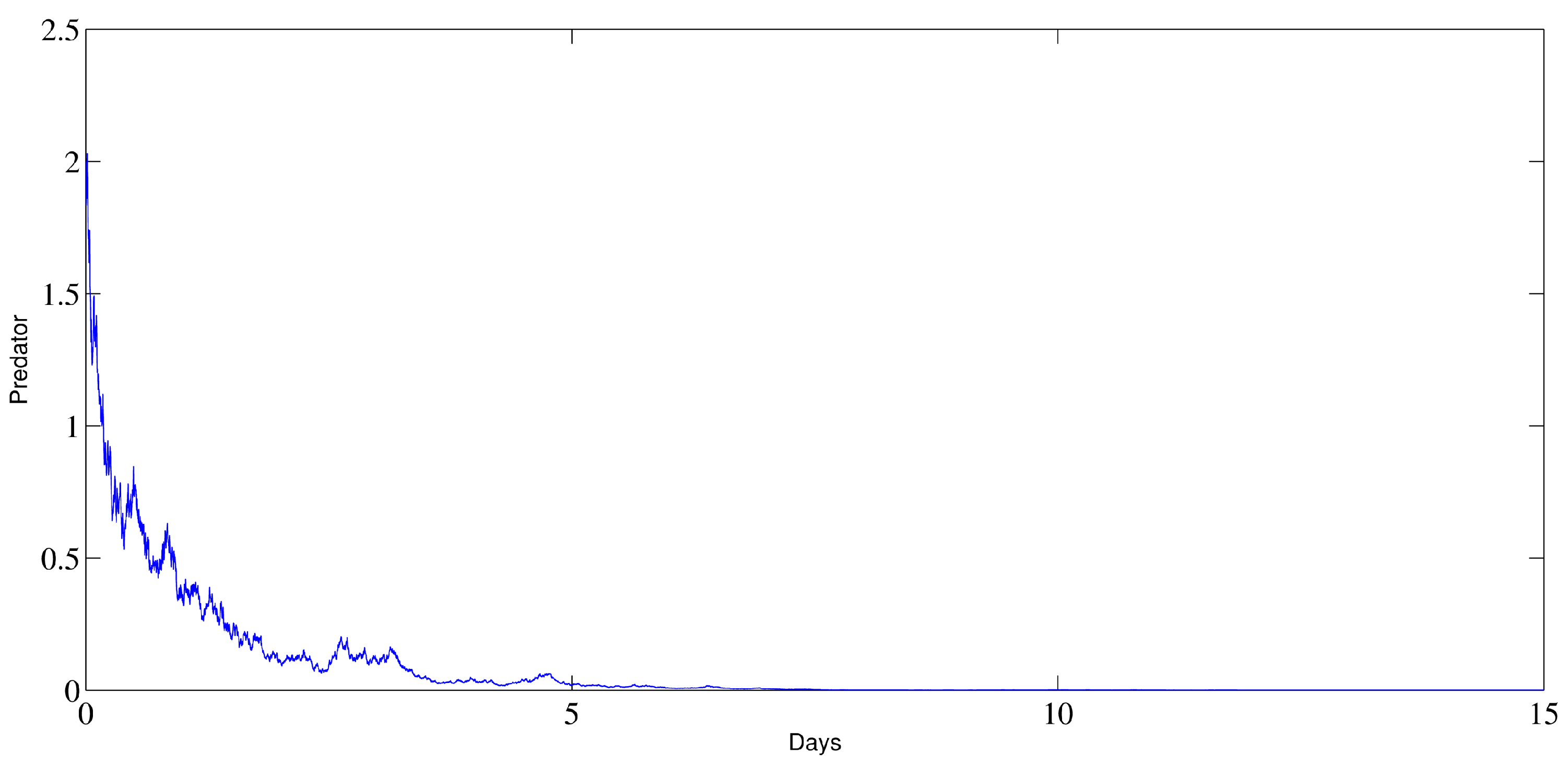
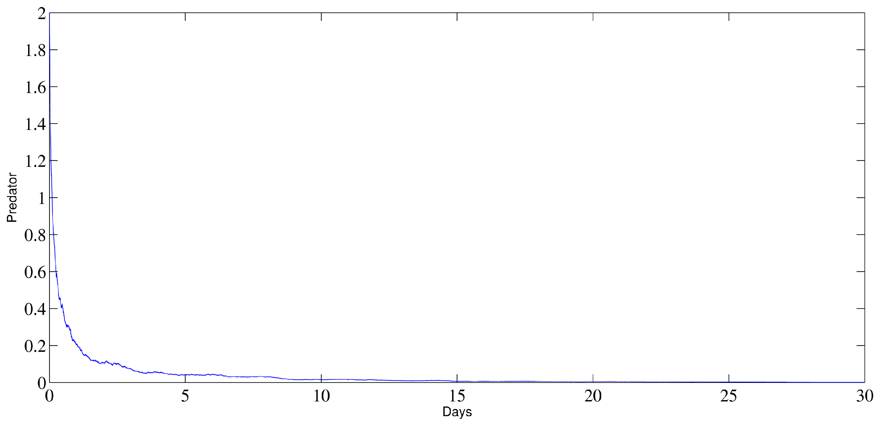
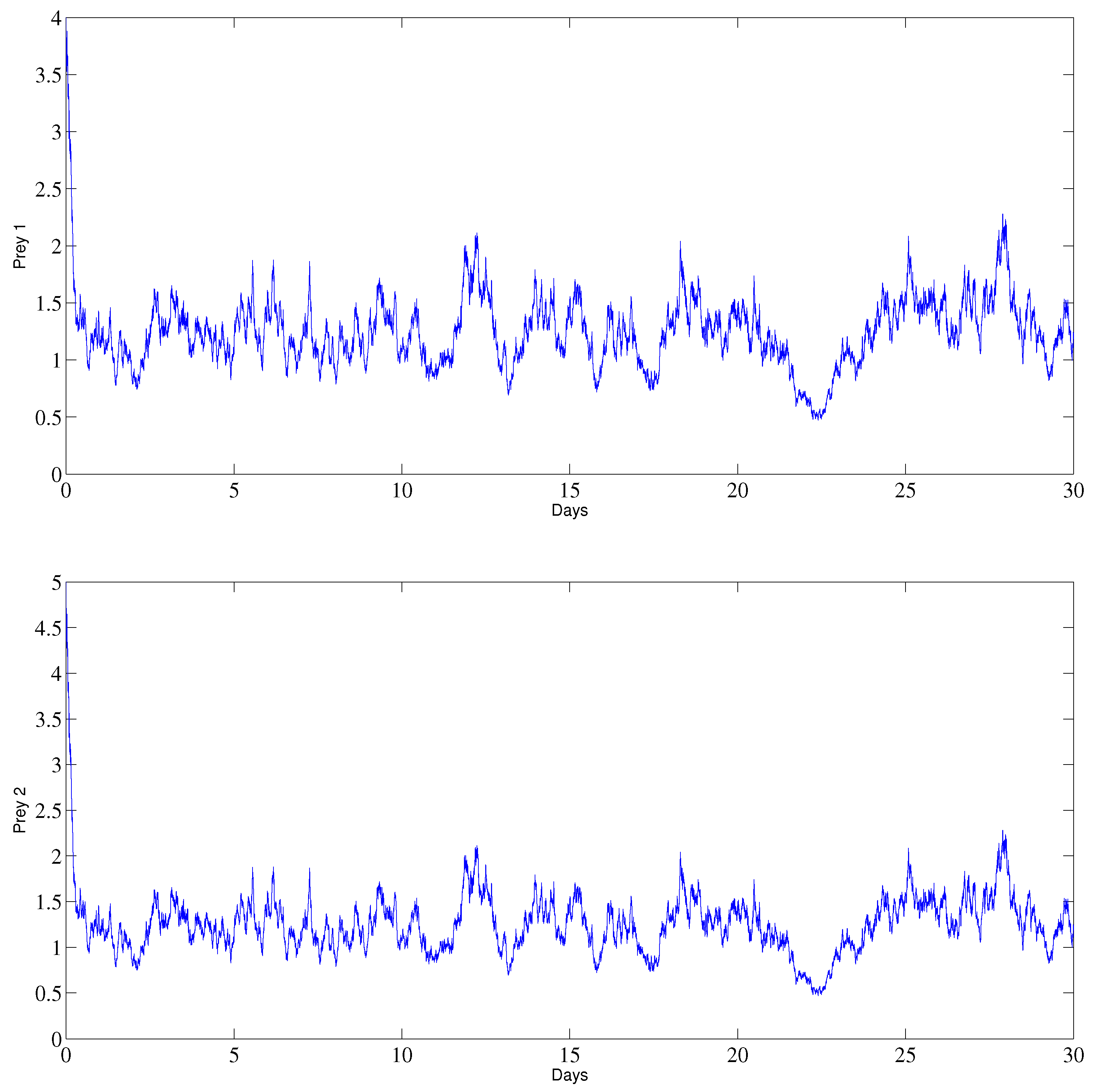
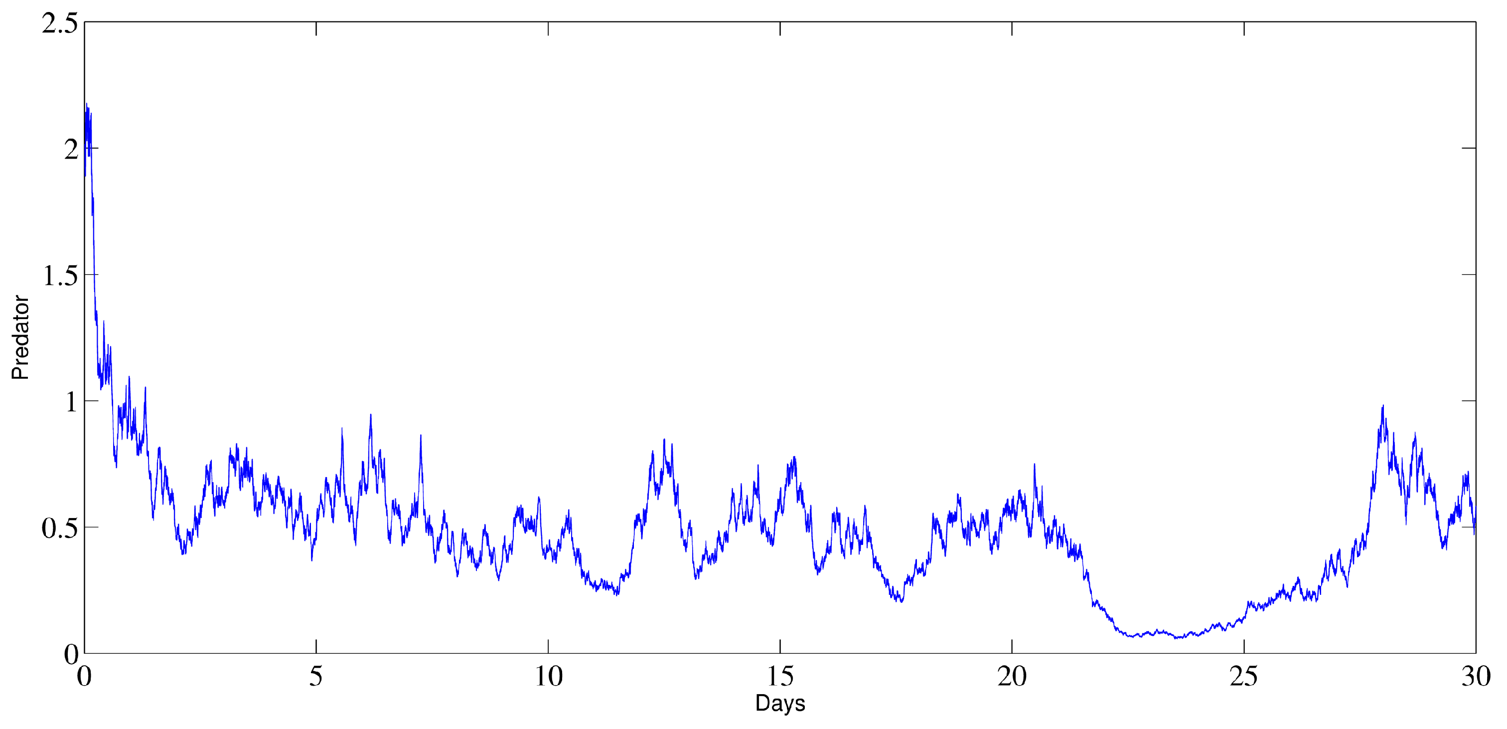
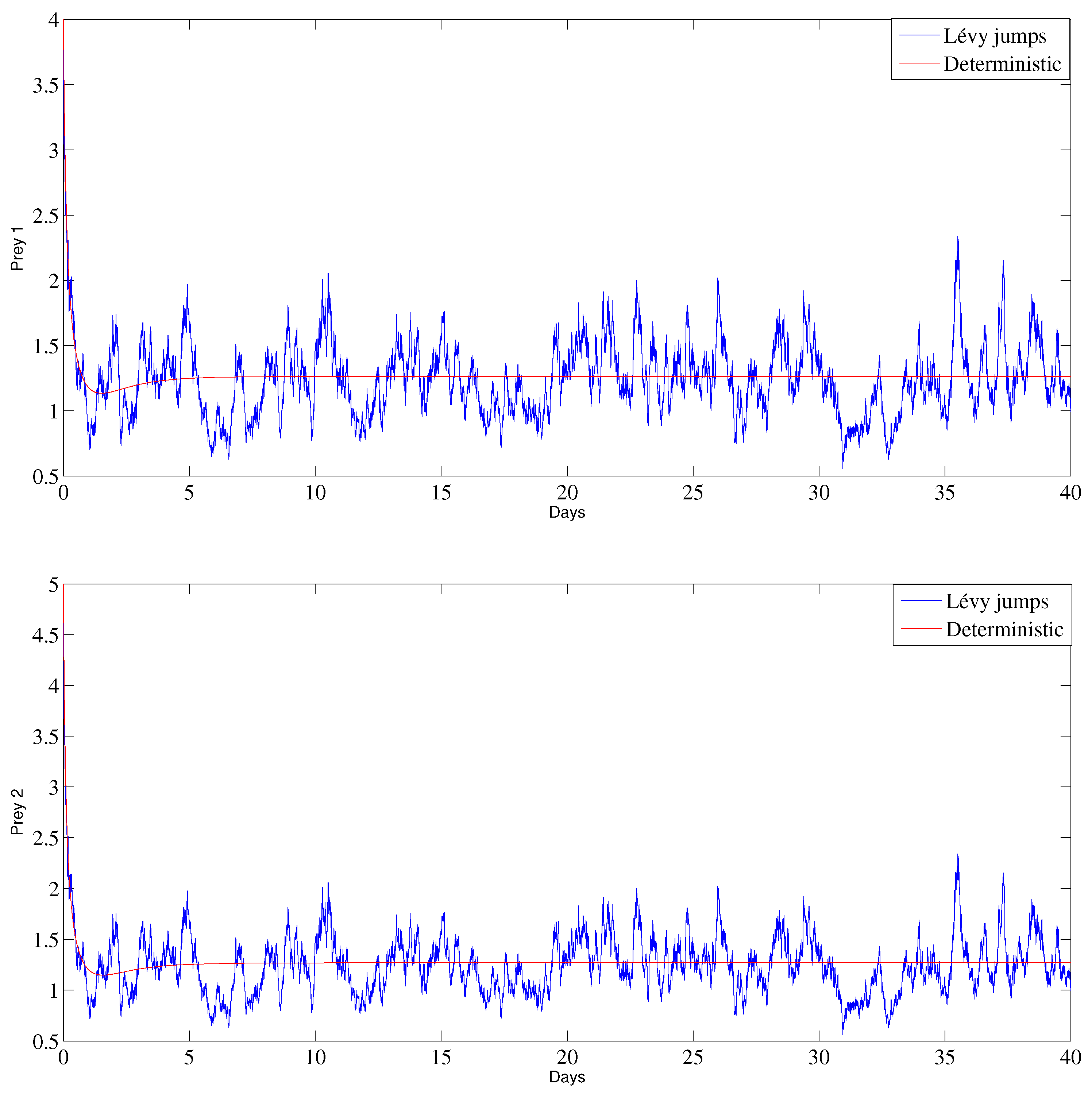
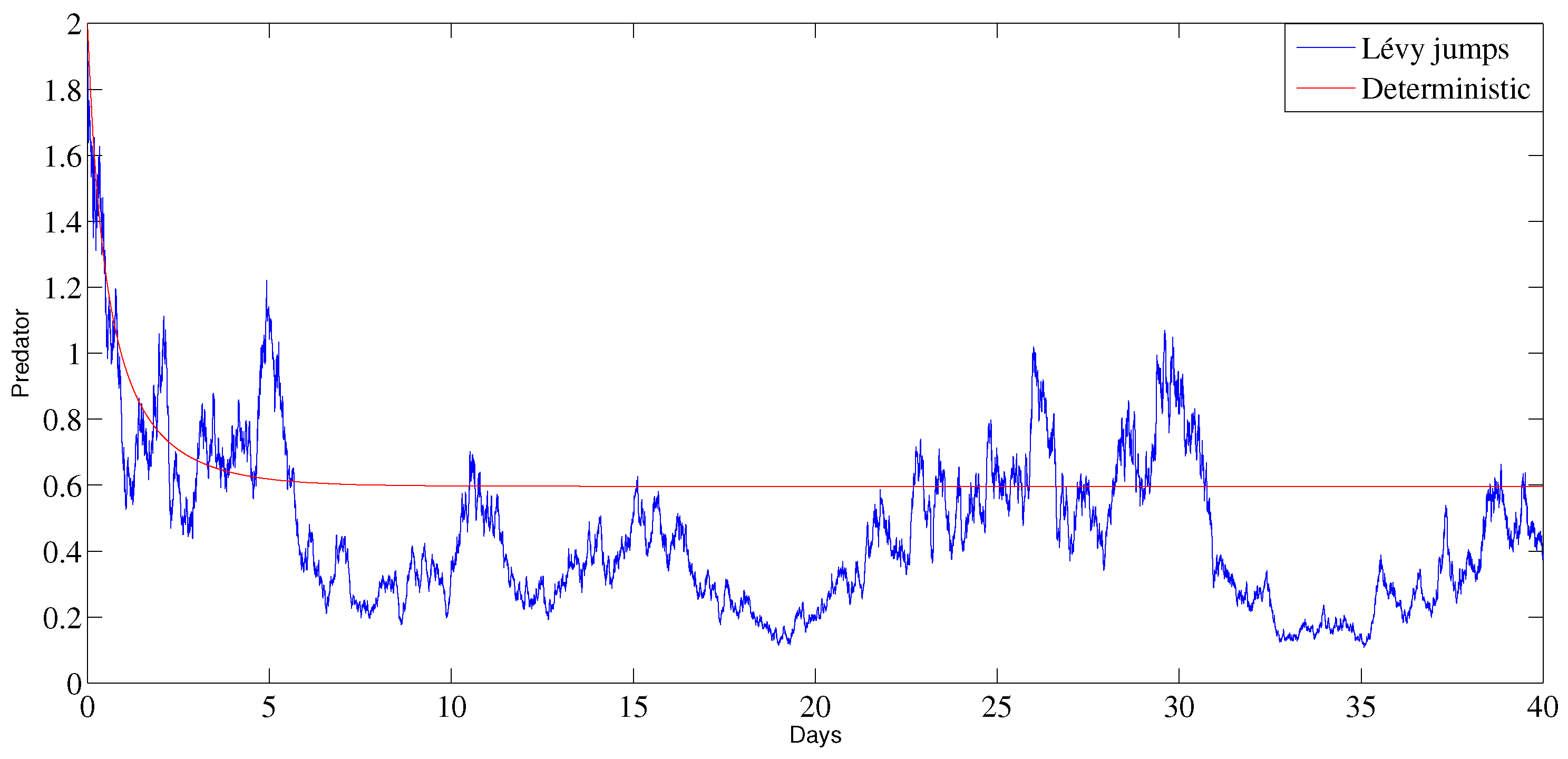
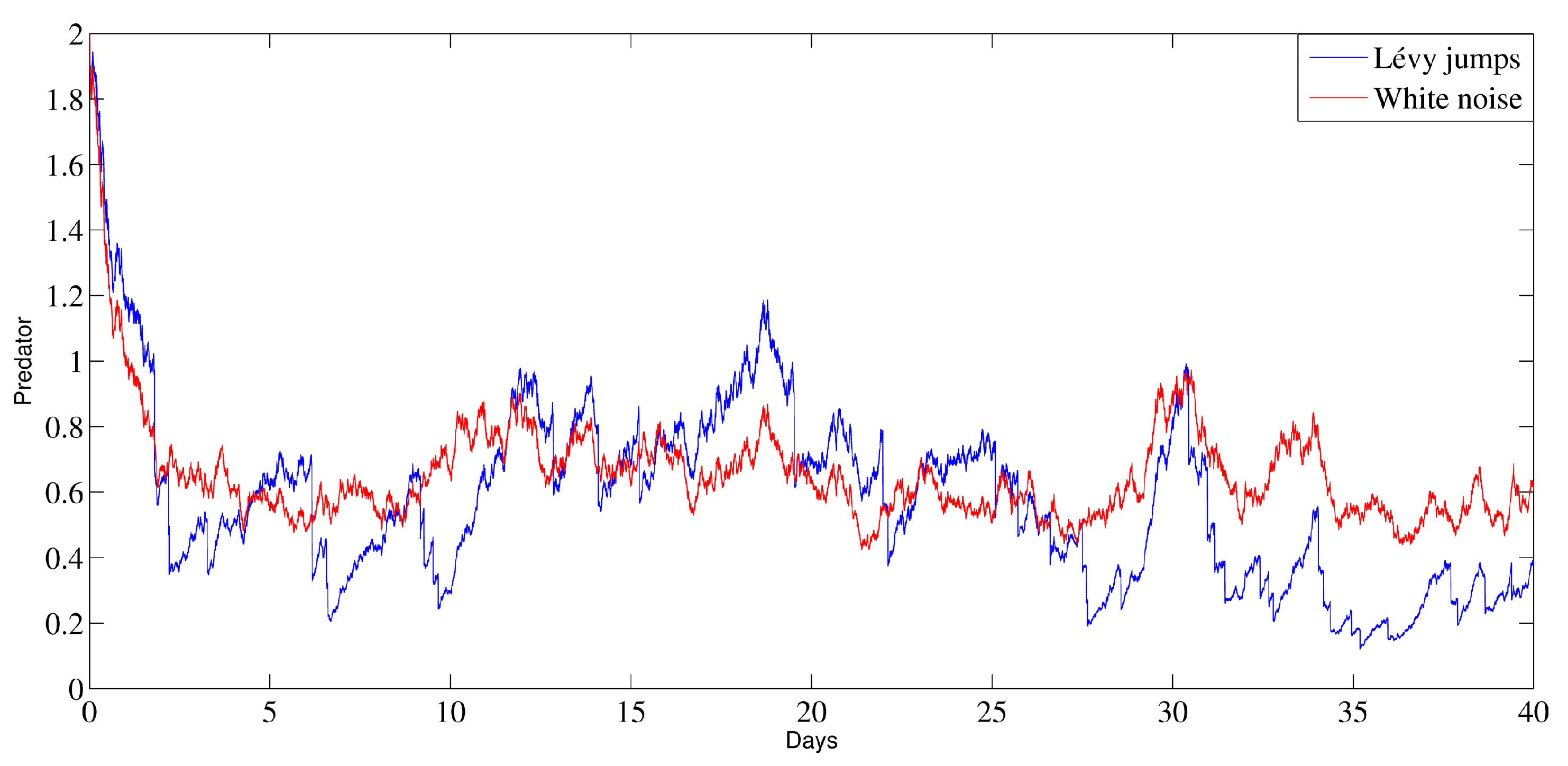
6. Numerical Analysis

In this section, we illustrate the algorithm used in the numerical analysis of the considered model (2). First, we use the following equation:

$$dZ\left(t\right)=\mathcal{G}\left(t,Z\left(t\right)\right)dt+\sigma \left(t,Z\left(t\right)\right)d{W}_t+{\int }_U\Pi (t,u)\mathcal{H}\left(t-,Z(t-)\right)\check{N}(dt,du).$$

(8)

Thus,

$$\begin{array}{cc}\hfill Z\left(t\right)& =Z\left(0\right)+\underset{\mathrm{Part}\mathrm{I}}{\underbrace{{\int }_0^t\mathcal{G}\left(\xi ,Z\left(\xi \right)\right)d\xi +{\int }_0^t\sigma \left(\xi ,Z\left(\xi \right)\right)d{W}_{\xi }}}\hfill \\ \hfill & +\underset{\mathrm{Part}\mathrm{II}}{\underbrace{\mathcal{H}\left(t-,Y(t-)\right){\int }_0^t{\int }_U\Pi (\xi ,u)\check{N}(d\xi ,du)}}.\hfill \end{array}$$

(9)

Using the Runge–Kutta method, we can provide an approximation of part I in (8):

$$\begin{array}{cc}\hfill Z_{j+1}& =Z_j+{\displaystyle \frac{1}{6}}\left(M_1+2M_2+2M_3+M_4\right),\hfill \end{array}$$

with

$$\begin{array}{cc}\hfill M_1& =\mathcal{G}(t_j,Z_j)h_t+\sigma (t_j,Z_j)(W_{j+1}-W_j),\hfill \\ \hfill M_2& =\mathcal{G}(t_j+\frac{h_t}{2}t,Z_j+\frac{M_1}{2})h_t+\sigma (t_j+\frac{h_t}{2},Z_j+\frac{M_1}{2})(W_{j+1}-W_j),\hfill \\ \hfill M_3& =\mathcal{G}(t_j+\frac{h_t}{2},Z_j+\frac{M_2}{2})h_t+\sigma (t_j+\frac{h_t}{2},Z_j+\frac{M_2}{2})(W_{j+1}-W_j),\hfill \\ \hfill M_4& =\mathcal{G}(t_j+h_t,Z_j+M_3)h_t+\sigma (t_j+h_t,Z_j+M_3)(W_{j+1}-W_j).\hfill \end{array}$$

We consider the infinitesimal interval $[T_j,T_{j+1})\subset (t_j,t_{j+1})$; then, for the second part, we have the following:

With no jumping on $[T_j,T_{j+1})$, we obtain

$$\mathcal{H}\left(t-,Z(t-)\right){\int }_{T_j}^{T_{j+1}}{\int }_U\Pi (\xi ,u)\check{N}(d\xi ,du)=0.$$

With one jump at the point $t_i\in [T_i,T_{i+1}),$ we obtain

$$\mathcal{H}\left(t-,Z(t-)\right){\int }_{T_j}^{T_{j+1}}{\int }_U\Pi \left(u\right)\check{N}(d\xi ,du)=\mathcal{H}\left(t_j-,Z(t_j-)\right)\Pi \left(t_j,\varsigma \left(t_j\right)\right),$$

and,

$$\mathcal{H}\left(t-,Z(t-)\right){\int }_0^t{\int }_U\Pi (\xi ,u)\check{N}(d\xi ,du)=\sum _{j=0}^{j=n}\mathcal{H}\left(t_i-,Z(t_j-)\right)\Pi \left(t_j,\varsigma \left(t_j\right)\right).$$

Therefore,

$$Z_{j+1}=Z_j+{\displaystyle \frac{1}{6}}\left(M_1^{\prime }+2M_2^{\prime }+2M_3^{\prime }+M_4^{\prime }\right)$$

is the Runge–Kutta version of Equation (8), with

$$\begin{array}{cc}\hfill M_1^{\prime }& =\mathcal{G}(t_j,Z_j)h_t+\sigma (t_j,Z_j)(W_{j+1}-W_j)\hfill \\ \hfill & +\mathcal{H}(t_j-,Z\left(t_j\right))\Pi (t_j,\varsigma \left(t_j\right)),\hfill \\ \hfill M_2^{\prime }& =\mathcal{G}(t_j+\frac{h_t}{2},Z_j+\frac{M_1^{\prime }}{2})h_t+\sigma (t_j+\frac{h_t}{2},Z_j+\frac{M_1^{\prime }}{2})(W_{j+1}-W_j)\hfill \\ \hfill & +\mathcal{H}(t_j+\frac{h_t}{2},Z(t_j)+\frac{M_1^{\prime }}{2})\Pi (t_j+\frac{h_t}{2},\varsigma (t_j+\frac{h_t}{2})),\hfill \\ \hfill M_3^{\prime }& =\mathcal{G}(t_j+\frac{h_t}{2},Z_j+\frac{M_2^{\prime }}{2})h_t+\sigma (t_j+\frac{h_t}{2},Y_j+\frac{M_2^{\prime }}{2})(W_{j+1}-W_j)\hfill \\ \hfill & +\mathcal{H}(t_J+\frac{h_t}{2},Z(t_j)+\frac{M_2^{\prime }}{2})\Pi (t_j+\frac{h_t}{2},\varsigma (t_j+\frac{h_t}{2})),\hfill \\ \hfill M_4^{\prime }& =\mathcal{G}(t_j+h_t,Z_j+M_3^{\prime })h_t+\sigma (t_j+h_t,Z_j+M_3^{\prime })(W_{j+1}-W_j)\hfill \\ \hfill & +f(t_j+h_t,Z\left(t_j\right)+M_3^{\prime })\Pi (t_j+h_t,\varsigma (t_j+h_t)).\hfill \end{array}$$

The different values used for the numerical results are provided in

Table 2. Values of the parameters used in the numerical simulations.

Parameters	Figure 1	Figure 2	Figure 3
${\upsilon }_1$	$0.7$	$1.7$	2
${\varrho }_1$	2	3	3
${\upsilon }_2$	$0.65$	$1.8$	$2.3$
${\varrho }_2$	1	4	4
${\vartheta }_1$	$0.1$	$0.15$	$0.2$
${\vartheta }_2$	$0.12$	$0.17$	$0.3$
${\varrho }_3$	2	2	$1.5$
$\beta$	$0.002$	$0.0015$	$0.001$
d	$0.4$	$0.35$	$0.1$
${\sigma }_1$	${10}^{-3}$	${10}^{-3}$	${10}^{-2}$
${\sigma }_2$	$2\times {10}^{-5}$	$2\times {10}^{-4}$	$2\times {10}^{-3}$
${\sigma }_3$	$2\times {10}^{-5}$	$2\times {10}^{-3}$	$2\times {10}^{-2}$
${\Xi }_1\left(u\right)$	$0.006$	$0.005$	$0.005$
${\Xi }_2\left(u\right)$	$0.03$	$0.03$	$0.03$
${\Xi }_3\left(u\right)$	$0.07$	$0.06$	$0.05$

.

The dynamics of the two prey subpopulations ${\mathcal{X}}_1$ and ${\mathcal{X}}_2$ and the predator subpopulation y can be seen in Figure 1, where the extinction of both prey species and the predator species can be observed.

Figure 2 illustrates the behavior of ${\mathcal{X}}_1$, ${\mathcal{X}}_2$ and y; it can be observed that the prey subpopulations remain strictly positive and the predator subpopulation vanishes, indicates the extinction of the predator and is opposite to the scenario in which the predator and prey populations persist.

The behavior of ${\mathcal{X}}_1$, ${\mathcal{X}}_2$ and y is illustrated in Figure 3, observing that all the considered populations persist, which coincides with our theoretical result in the case of persistence.

In Figure 4, we show a comparison between the stochastic model (2) and deterministic model (1) in the persistence case. It can be observed that the curve of the stochastic case has perturbations around the deterministic curve, which proves that the stochastic model can more efficiently describe the dynamics of the prey–predator model.

Figure 5 shows a comparison of the stochastic model (2) in the persistence case with and without Lévy jumps. It is notable that the curve of the stochastic model with jumping has a number of jumped-up perturbations, while the curve without Lévy jumps has normal perturbations. This observation demonstrates that certain cases can lead to Lévy jumps in the behavior of the prey–predator model.

7. Conclusions and Discussion

This paper has investigated a stochastic prey–predator model driven by Lévy noise in the presence of two prey subpopulations and one predator subpopulation. The model under consideration uses two forms of functional responses, namely, Holling-II ${\displaystyle \frac{y{\mathcal{X}}_2}{{\iota }_2+{\mathcal{X}}_2+\beta y}}$ and Beddington–DeAngelis ${\displaystyle \frac{y{\mathcal{X}}_1}{{\iota }_1+{\mathcal{X}}_1}}$, due to the saturation behavior. These two mixed functionals can better describe the reality of the computation between the prey and predator subpopulations. First, we have established the well-posedness of the solution of the model (2). An analysis of persistence and extinction led us to three possible cases: the first is devoted to the extinction of all the considered population when $max\{m_1,m_2,m_3\}\le 0$; the second case is dedicated to the persistence of the two prey species and the extinction of the predator species when $min\{m_1^{\prime },m_2^{\prime }\}\ge 0$ and $m_4\le 0$; and in the last case, we show the persistence of all the studied populations under several conditions. In our numerical analysis, we illustrate a special Runge–Kutta method for the stochastic model under Brownian and Lévy jump perturbations as implemented in Matlab R2019b software.

In this way, we considered the three cases with respect to extinction (persistence of the two prey species, extinction of the predator, and persistence of all three species) in simulations in order to validate our theoretical findings. Finally, we present several numerical comparisons. The first is between the deterministic and stochastic cases, which shows the usefulness of considering the stochastic model. The second comparison is between the cases with and without Lévy jumps, which proves that certain cases naturally lead to Lévy jumping in the behavior of the prey–predator model. Future efforts should address remaining issues; one of these is how the presented predator-prey model spreads via Levy jumps. In addition, we intend to study the chaotic behavior of the stochastic predator–prey system. Moreover, it is possible to model the prey–predator relationship using the space–time spectral order Sinc-collocation method (see [36] for example) and to illustrate a new modified stochastic predictor–corrector compact difference method, such as the one suggested in [38].

References

1. Naik, P.A.; Eskandari, Z.; Shahkari, H.E.; Owolabi, K.M. Bifurcation analysis of a discrete-time prey–predator model. Bull. Biomath. 2023, 1, 111–123. [Google Scholar] [CrossRef]
2. Chatterjee, A.; Pal, S. A predator–prey model for the optimal control of fish harvesting through the imposition of a tax. Int. J. Optim. Control Theor. Appl. 2023, 13, 68–80. [Google Scholar] [CrossRef]
3. Tripathi, J.P.; Tyagi, S.; Abbas, S. Global analysis of a delayed density dependent predator–prey model with Crowley-Martin functional response. Commun. Nonlinear Sci. Numer. Simul. 2016, 30, 45–69. [Google Scholar] [CrossRef]
4. Naik, P.A.; Eskandari, Z.; Yavuz, M.; Zu, J. Complex dynamics of a discrete-time Bazykin–Berezovskaya prey-predator model with a strong Allee effect. J. Comput. Appl. Math. 2022, 413, 114401. [Google Scholar] [CrossRef]
5. Lotka, A. Elements of Mathematical Biology; Dover Publications: New York, NY, USA, 1956. [Google Scholar]
6. Spencer, P.D.; Collie, J.S. A simple predator–prey model of exploited marine fish populations incorporating alternative prey. ICES J. Mar. Sci. 1996, 53, 615–628. [Google Scholar] [CrossRef]
7. Fay, T.H.; Greeff, J.C. Lion, wildebeest and zebra: A predator–prey model. Ecol. Model. 2006, 196, 237–244. [Google Scholar] [CrossRef]
8. Verhulst, P.F. Notice sur la loi que la population suit dans son accroissement. Corresp. MathéMatique Phys. 1838, 10, 113–121. [Google Scholar]
9. Pearl, R.; Reed, L.J. The logistic curve and the census count of i930. Science 1930, 72, 399–401. [Google Scholar] [CrossRef] [PubMed]
10. MacLean, M.; Willard, A. The logistic curve applied to Canada’s population. Can. J. Econ. Polit. Sci. 1937, 3, 241–248. [Google Scholar] [CrossRef]
11. Kot, M. Elements of Mathematical Ecology; Cambridge University Press: Cambridge, UK, 2001. [Google Scholar]
12. Kingsland, S. The refractory model: The logistic curve and the history of population ecology. Q. Rev. Biol. 1982, 57, 29–52. [Google Scholar] [CrossRef]
13. Keshet, E.L. Mathematical Models in Biology; McGrawHill: New York, NY, USA, 1988. [Google Scholar]
14. Ghosh, D.; Santra, P.K.; Mahapara, G.S. A three-component prey-predator system with interval number. Math. Model. Numer. Simul. Appl. 2023, 3, 1–16. [Google Scholar] [CrossRef]
15. Yavuz, M.; Sene, N. Stability analysis and numerical computation of the fractional predator–prey model with the harvesting rate. Fractal Fract. 2020, 4, 35. [Google Scholar] [CrossRef]
16. Meng, X.Y.; Huo, H.F.; Xiang, H.; Yin, Q.Y. Stability in a predator–prey model with Crowley-Martin function and stage structure for prey. Appl. Math. Comput. 2014, 232, 810–819. [Google Scholar] [CrossRef]
17. Ko, W.; Ryu, K. Qualitative analysis of a predator—Prey model with Holling type II functional response incorporating a prey refuge. J. Differ. Equ. 2006, 231, 534–550. [Google Scholar] [CrossRef]
18. Sugie, J.; Kohno, R.; Miyazaki, R. On a predator-prey system of Holling type. Proc. Am. Math. Soc. 1997, 125, 2041–2050. [Google Scholar] [CrossRef]
19. Baek, H.; Dongseok, K. Dynamics of a predator-prey system with mixed functional responses. J. Appl. Math. 2014, 2014, 536019. [Google Scholar] [CrossRef]
20. Zou, X.; Li, Q.; Cao, W.; Lv, J. Thresholds and critical states for a stochastic predator–prey model with mixed functional responses. Math. Comput. Simul. 2023, 206, 780–795. [Google Scholar] [CrossRef]
21. Liu, Q.; Jiang, D.; Hayat, T.; Alsaedi, A. Dynamics of a stochastic predator–prey model with stage structure for predator and Holling type II functional response. J. Nonlinear Sci. 2018, 28, 1151–1187. [Google Scholar] [CrossRef]
22. Rihan, F.A.; Alsakaji, H.J. Stochastic delay differential equations of three-species prey-predator system with cooperation among prey species. Discret. Contin. Dyn.-Syst. 2020, 15, 245–263. [Google Scholar] [CrossRef]
23. Danane, J.; Allali, K.; Hammouch, Z.; Nisar, K.S. Mathematical analysis and simulation of a stochastic COVID-19 Lévy jump model with isolation strategy. Results Phys. 2021, 23, 103994. [Google Scholar] [CrossRef] [PubMed]
24. Akdim, K.; Ez-zetouni, A.; Danane, J.; Allali, K. Stochastic viral infection model with lytic and nonlytic immune responses driven by Lévy noise. Phys. Stat. Mech. Its Appl. 2020, 549, 124367. [Google Scholar] [CrossRef]
25. Danane, J. Stochastic predator–prey Lévy jump model with Crowley–Martin functional response and stage structure. J. Appl. Math. Comput. 2021, 67, 41–67. [Google Scholar] [CrossRef]
26. Zhao, S.; Song, M. A stochastic predator-prey system with stage structure for predator. Abstr. Appl. Anal. 2014, 2014, 518695. [Google Scholar] [CrossRef]
27. Danane, J. Stochastic Capital–Labor Lévy Jump Model with the Precariat Labor Force. Math. Comput. Appl. 2022, 27, 93. [Google Scholar] [CrossRef]
28. Choo, S.; Kim, Y.H. Global stability in stochastic difference equations for predator-prey models. J. Comput. Anal. Appl. 2017, 23, 3. [Google Scholar]
29. Yang, L.; Zhong, S. Global stability of a stage-structured predator-prey model with stochastic perturbation. Discret. Dyn. Nat. Soc. 2014, 2014, 512817. [Google Scholar] [CrossRef]
30. Zhao, Y.; Yuan, S. Stability in distribution of a stochastic hybrid competitive Lotka–Volterra model with Lévy jumps. Chaos Solitons Fractals 2016, 85, 98–109. [Google Scholar] [CrossRef]
31. Liu, Q.; Chen, Q.M. Analysis of a stochastic delay predator-prey system with jumps in a polluted environment. Appl. Math. Comput. 2014, 242, 90–100. [Google Scholar] [CrossRef]
32. Zhang, X.; Li, W.; Liu, M.; Wang, K. Dynamics of a stochastic Holling II one-predator two-prey system with jumps. Phys. Stat. Mech. Its Appl. 2015, 421, 571–582. [Google Scholar] [CrossRef]
33. Liu, M.; Bai, C.; Deng, M.; Du, B. Analysis of stochastic two-prey one-predator model with Lévy jumps. Phys. A Stat. Mech. Its Appl. 2016, 445, 176–188. [Google Scholar] [CrossRef]
34. Sabbar, Y. Asymptotic extinction and persistence of a perturbed epidemic model with different intervention measures and standard lévy jumps. Bull. Biomath. 2023, 1, 58–77. [Google Scholar] [CrossRef]
35. Mouhcine, N.; Sabbar, Y.; Anwar, Z. Stability characterization of a fractional-order viral system with the non-cytolytic immune assumption. Math. Model. Numer. Simul. Appl. 2022, 2, 164–176. [Google Scholar]
36. Wu, J. Stability of a three-species stochastic delay predator–prey system with Lévy noise. Phys. Stat. Mech. Appl. 2018, 502, 492–505. [Google Scholar] [CrossRef]
37. Hudson, R.L.; Parthasarathy, K.R. Quantum Ito’s formula and stochastic evolutions. Commun. Math. Phys. 1984, 93, 301–323. [Google Scholar] [CrossRef]
38. Jiang, X.; Wang, J.; Wang, W.; Zhang, H. A Predictor–Corrector Compact Difference Scheme for a Nonlinear Fractional Differential Equation. Fractal Fract. 2023, 7, 521. [Google Scholar] [CrossRef]
Figure 1. The behavior of the prey and predator subpopulations in the extinction situation.
Fractalfract 07 00751 g001aFractalfract 07 00751 g001b
Figure 2. The behavior of the prey and predator populations in the extinction–persistence situation.
Fractalfract 07 00751 g002aFractalfract 07 00751 g002b
Figure 3. The behavior of the prey and predator populations in the case of persistence.
Fractalfract 07 00751 g003aFractalfract 07 00751 g003b
Figure 4. Comparison of the behavior of the prey and predator populations the deterministic model and stochastic model in the case of persistence between.
Fractalfract 07 00751 g004aFractalfract 07 00751 g004b
Figure 5. Comparison of the behavior of the prey and predator populations in the case of persistence with and without Lévy jumps.
Fractalfract 07 00751 g005aFractalfract 07 00751 g005b