Article

On Stability of a Fractional Discrete Reaction–Diffusion Epidemic Model

1
Department of Mathematics, Faculty of Science, The Hashemite University, Zarqa 13133, Jordan
2
Laboratory of Dynamical Systems and Control, University of Oum EL-Bouaghi, Oum El Bouaghi 04000, Algeria
3
Department of Mathematics, Faculty of Science, Zarqa University, Zarqa 13110, Jordan
4
Applied Science Research Center (ASRC), Applied Science Private University, Amman 11931, Jordan
5
Department of Data Sciences and Artificial Intelligence, Al-Ahliyya Amman University, Amman 19111, Jordan
6
Department of Basic Scientific Sciences, Applied Science Private University, Amman 11931, Jordan
7
Department of Mathematics, Jerash University, Jerash 26150, Jordan
8
Department of Mathematics, Faculty of Science and Technology, Irbid National University, Irbid 2600, Jordan
9
Department of Mathematics and Computer Science, University of Oum EL-Bouaghi, Oum El Bouaghi 04000, Algeria
*
Author to whom correspondence should be addressed.
Fractal Fract. 2023, 7(10), 729; https://doi.org/10.3390/fractalfract7100729
Submission received: 29 July 2023 / Revised: 17 September 2023 / Accepted: 19 September 2023 / Published: 2 October 2023
(This article belongs to the Special Issue Advances in Fractional Modeling and Computation)

Abstract

:
This paper considers the dynamical properties of a space and time discrete fractional reaction–diffusion epidemic model, introducing a novel generalized incidence rate. The linear stability of the equilibrium solutions of the considered discrete fractional reaction–diffusion model has been carried out, and a global asymptotic stability analysis has been undertaken. We conducted a global stability analysis using a specialized Lyapunov function that captures the system’s historical data, distinguishing it from the integer-order version. This approach significantly advanced our comprehension of the complex stability properties within discrete fractional reaction–diffusion epidemic models. To substantiate the theoretical underpinnings, this paper is accompanied by numerical examples. These examples serve a dual purpose: not only do they validate the theoretical findings, but they also provide illustrations of the practical implications of the proposed discrete fractional system.

1. Introduction

In recent decades, fractional differential equation models have gained extensive attention within research fields. The prevalence of these models across a wide spectrum of applications, encompassing fields like biological mathematics, physics, and biology, has significantly motivated their exploration. Notably, the domain of nonlinear dynamics has increasingly turned its focus to fractional models, inspiring a surge of relevant research pursuits. For those intrigued by these developments, valuable insights can be gleaned from references such as [1,2,3,4,5,6,7,8].
Fractional reaction–diffusion order models are a generalization of traditional integer reaction–diffusion order models. It must be emphasized that they have benefits over standard integer-order reaction–diffusion models due to the fact that they have memory and genetic qualities that these latter models, which are commonly used by many biological systems, do not have. In addition, these models describe models of population with greater precision than integer-order models [9,10,11,12,13].
In reality, the transmission of infectious illnesses is affected not just by their present condition, but also by their former status. Since each fractional derivative comprises a kernel function, it is possible to conclude that the present state of fractional epidemic systems is dependent on previous data [14]. More notably, Angstmann et al. introduced an infectiousness fractional SIR system and demonstrated how fractional derivatives automatically arise from continuous random walks [15]. Hethcote presented a fractional SIR system with a constant population as a generalization of traditional integer ones [16]. The local stability of both equilibriums of a fractional SEIR epidemic system was then investigated in [17].
Except in rare instances where obtaining an explicit solution for diffusion fractional differential equations proves challenging, the possibilities extend to the study of both numerical and exact solutions based on the partial differential equation. In scenarios where the exact solution is elusive, recourse to the numerical solution remains a viable approach. Not only that, but discrete models have a unique physical process. [18,19,20,21,22]. In particular, infectious illness data are not continuous; however, they cover a specific time period. Furthermore, because the discrete representation of infectious illnesses can be in any time step for the unit, the continuous model is appropriate for easier and more efficient data following the discretization of the epidemic model (see [23,24,25,26]). Nonetheless, previous research on discrete epidemic systems either did not account for any types of diffusion or exclusively studied conventional diffusion. A noteworthy observation relates to the exploration of fractional discrete models coupled with diffusion, which has accumulated significant attention in the research fields. For instance, the work presented in [27] explores the advancement of a fractional discrete reaction–diffusion Lengyel–Epstein system, as well as a detailed examination of its asymptotic stability. Furthermore, the literature includes the presentation of a fractional discrete diffusion equation in [28], providing a unique path for further exploration. An intriguing work explores the chaotic dynamics of a variable-order fractional diffusion equation across non-continuous time scales, as detailed in [29]. The area of epidemic systems with discrete fractions combined with reaction–diffusion processes has been comprehensively explored in [30], uncovering the complexities of their behavior. These efforts together enhance our grasp of the interaction between fractional dynamics and diffusion phenomena. For a more comprehensive exploration into the dynamics of fractional discrete reaction–diffusion models, one can find additional insights in [31,32,33].
Inspired by prior research, we conduct a detailed study of a discrete fractional epidemic system with reaction–diffusion, featuring a generalized incidence rate. In this study, we uncover essential insights that play a key role in our investigation:
  • At the core of our investigation is the introduction of a new discrete fractional epidemic model. This model is created by skillfully combining the L1 scheme and the second-order central difference scheme, which effectively transforms the continuous model into its discrete form. This transformation results in a carefully crafted discrete model, laying the foundation for our subsequent analyses.
  • Central to our study is a thorough examination of both the local and global asymptotic stability within the proposed fractional discrete reaction–diffusion epidemic model. We employ a powerful linearization technique to analyze the complex stability characteristics near equilibrium points. To establish global stability, we utilize a Lyapunov function that effectively captures historical data, strengthening the reliability of our findings.
  • The theoretical framework resulting from our analyses strongly aligns with real-world dynamics. This alignment is robustly confirmed through a series of simulations, where the practical significance of our theoretical discoveries becomes evident. The simulations clearly validate the substantial influence of our findings on the complex network of disease transmission dynamics.
Below is a detailed elaboration of how our work is organized, including every crucial aspect: Within Section 2, we start an important step by generating the discrete form of the fractional reaction–diffusion epidemic system. This process is achieved through the skillful application of the second-order central difference scheme and the L1 scheme. This section is fundamental for the following analyses and investigations that will take place. Section 3 represents a crucial point where we start identifying equilibrium points within the investigated epidemic system. Moreover, we introduce and compute the fundamental reproduction number—an essential metric that Describes how the system spreads. This section sets the foundation for our subsequent explorations of stability. Our investigation advances to Section 4, where we engage in a detailed analysis of the local asymptotic stability. We explore various scenarios both with and without diffusion, all centered around the fundamental reproduction number. This section dissects the stability properties of equilibrium points under varying conditions, enriching our understanding of the system’s dynamics. In Section 5, our attention turns to the global stability analysis of the system. We utilize a well-suited Lyapunov functional to unravel the stability of both the disease-free and epidemic equilibrium points. This section offers a profound perspective on the long-term behavior of the system, highlighting its lasting characteristics. Section 6 connects theory with real-world application through the presentation of examples and simulations. Through these illustrative instances, we illustrate the theoretical ideas in real-world situations, allowing readers to see how they work. This section demonstrates the practical utility of our approach. In Section 7, to conclude, we review our research path and summarize the key insights gathered from each preceding section. We also offer insights into potential directions for future research, providing a comprehensive conclusion that covers both the outcomes of our work and its potential implications.

2. A Novel Fractional Discrete-Time Reaction–Diffusion Epidemic Model

Numerous studies on fractional anomalous diffusion models of infectious diseases have been published [14,15,16,17]. In particular, Zhen et al. examined a class of reaction–diffusion by generalizing the incidence rate fractional-order SIR epidemic model in [34] as follows:
0 C D t α S = k 1 Δ S + θ γ S ψ ( I ) ϵ S , t > 0 , x Ω , 0 C D t α I = k 2 Δ I + γ S ψ ( I ) ( ν + σ ) I , t > 0 , x Ω , 0 C D t α R = k 3 Δ R + σ I δ R , t > 0 , x Ω ,
where the investigated population includes both vulnerable individuals S and infected individuals I. θ reflects the flow rate of recently exposed persons; the symbol ϵ is the mortality rate; the parameter γ defines the rate of disease prevalent within individuals per unit time; and the constant σ is provided by σ = ϵ + ν , where 1 ν is the mean length of a sexual encounter among affected individuals.
k 1 and k 2 represent the diffusion coefficients, and Δ is the Laplacian operator on Ω , where Ω R n is a bounded subset of R n with a smooth border Ω and with homogeneous Neumann boundary conditions and initial conditions.
S ( x , 0 ) = S 0 ( x ) , I ( x , 0 ) = I 0 ( x ) , R ( x , 0 ) = R 0 ( x ) .
It goes without saying that the nonlinearity ψ is a positive and continuously differentiable functional on R + such that
ψ ( 0 ) = 0 ,
and
0 < I ψ ( I ) ψ ( I ) , I > 0 .
However, it has been reported that the recovered class R of System (1) has no effect on the susceptible class S or the infected class I. As a result, the study in [34] concentrated on the following reduced system:
0 C D t α S = k 1 Δ S + θ γ S ψ ( I ) ϵ S , t > 0 , x Ω , 0 C D t α I = k 2 Δ I + γ S ψ ( I ) ( ν + σ ) I , t > 0 , x Ω .
Hence, the discretization and dynamics in this work are based on the epidemic model (5). Because real-world data are discrete, the discrete system is better suited to simulating the spread of disease, based on System (5) and the discretization approach used in [28]. When x [ 0 , L ] , we obtain x i + 1 = x i + d x , i = 0 , , m , and by using the central difference formula for x , 2 S ( x , t ) x 2 and 2 I ( x , t ) x 2 are estimated by
2 S ( x , t ) x 2 S i + 1 ( t ) 2 S i ( t ) + S i 1 ( t ) d x 2 , 2 I ( x , t ) x 2 I i + 1 ( t ) 2 I i ( t ) + I i 1 ( t ) d x 2 .
Considering the definition of the second-order difference operator of S i and I i described in [35,36] by
Δ 2 y ( r ) = y ( r + 2 ) 2 y ( r + 1 ) + y ( r ) , r N .
We obtain the following approximations:
2 S ( x , t ) x 2 Δ 2 S i 1 ( t ) d x 2 , 2 I ( x , t ) x 2 Δ 2 I i 1 ( t ) d x 2 .
Consequently, we take into consideration the following discrete fractional reaction–diffusion epidemic model:
C Δ t 0 ξ S i ( t ) = k 1 d x 2 Δ 2 S i 1 ( t + ξ ) + θ γ S i ( t + ξ ) ψ ( I i ( t + ξ ) ) ϵ S i ( t + ξ ) , C Δ t 0 ξ I i ( t ) = k 2 d x 2 Δ 2 I i 1 ( t + ξ ) + γ S i ( t + ξ ) ψ ( I i ( t + ξ ) ) ( ν + σ ) I i ( t + ξ ) .
To simplify our simulations and ensure that edge effects do not interfere with our results, we will utilize periodic boundary conditions, following the approach outlined in [28].
S 0 ( t ) = S m ( t ) , S 1 ( t ) = S m + 1 ( t ) , I 0 ( t ) = I m ( t ) , I 1 ( t ) = I m + 1 ( t ) ,
and the initial condition
S i t 0 = Φ 1 x i 0 , I i t 0 = Φ 2 x i 0 .
while the definition of the Caputo -difference operator is as follows:
Definition 1
([37,38]). The Caputo ℏ-difference operator is denoted by
C Δ a α y ( t ) = Δ a ( n α ) Δ n y ( t ) , t ( N ) a + α , 0 < α < 1 ,
and the α-th order ℏ-sum is described by
Δ a α y ( t ) = Γ ( α ) t α s = a ( t σ ( s ) ) ( α 1 ) y ( s ) , σ ( s ) = ( s + 1 ) ,
with the set ( N ) a + α defined by
( N ) a + α = { a + ( 1 α ) , a + ( 2 α ) , } .

3. Fixed Points and Basic Reproduction Number

3.1. Fixed Points

Identifying the fixed points is a prerequisite for studying the dynamics of System (9), and the following nonlinear system needs to be solved in order to do so:
θ γ S i ( t + ξ ) ψ ( I i ( t + ξ ) ) ϵ S i ( t + ξ ) = 0 , γ S i ( t + ξ ) ψ ( I i ( t + ξ ) ) ( ν + σ ) I i ( t + ξ ) = 0 .
The point E 0 = θ ϵ , 0 is a solution to the previous system. Since the disease is nonexistent, E 0 is referred to as the disease-free fixed point.
Now, considering that I > 0 , we have
S * = θ ϵ ( ν + σ ) I * ϵ .
The point E * = ( S * , I * ) is called the epidemic equilibrium point; its existence may be explored numerically.

3.2. Basic Reproduction Number

For the purpose of understanding how epidemic systems behave, the fundamental reproduction number is crucial. Ref. [39] states that the fundamental reproduction number is the spectral radius of the subsequent generation matrix F V 1 , wherein F and V are the Jacobian matrices for F and V 1 , respectively, at the disease-free fixed point, and where F is the rate at which new infections appear:
F = γ S ψ ( I ) 0 ,
and V , the infection disappearance rate:
V = ( ν + σ ) I θ + γ S ψ ( I ) + ϵ S .
Hence, the Jacobite matrices at the disease-free equilibrium E 0 are as follows:
F = θ ϵ γ ψ ( 0 ) 0 0 0 , V = ν + σ 0 θ ϵ γ ψ ( 0 ) ϵ ,
The fundamental reproductive number, based on the Jacobite matrices, is provided by:
R 0 = γ θ ϵ ( ν + σ ) ψ ( 0 ) .

4. Local Stability

4.1. Local Stability of the Free Diffusion Epidemic Model

We now provide adequate requirements for the local asymptotic stability of the two equilibriums of the following system:
C Δ t 0 ξ S ( t ) = θ γ S ( t + ξ ) ψ ( I ( t + ξ ) ) ϵ S ( t + ξ ) , C Δ t 0 ξ I ( t ) = γ S ( t + ξ ) ψ ( I ( t + ξ ) ) ( ν + σ ) I ( t + ξ ) .
with the initial conditions
S ( t 0 ) = S 0 > 0 , I ( t 0 ) = I 0 > 0 .
We require the following theorem before we can investigate local stability:
Theorem 1
([40]). Let ( S * , I * ) represent the equilibrium point of (19). If all of the eigenvalues of J E * are in S α , then ( S * , I * ) is asymptotically stable.
where
S α = w C : | A r g ( w ) | > α π 2 or | w | > 2 α α cos α A r g ( w ) α .
Theorem 2.
If R 0 < 1 , the disease-free fixed point E 0 is asymptotically stable.
If R 0 > 1 , the epidemic equilibrium point E * is asymptotically stable.
Proof. 
First, we establish the Jacobian matrix of System (19)
J = γ ψ ( I ( t + ξ ) ) ϵ γ S ( t + ξ ) ψ ( I ( t + ξ ) ) γ ψ ( I ( t + ξ ) ) γ S ( t + ξ ) ψ ( I ( t + ξ ) ) ( ν + σ ) .
  • The Jacobian matrix at the free disease point E 0
    J E 0 = ϵ θ ϵ ψ ( 0 ) γ 0 θ ϵ ψ ( 0 ) γ ( ν + σ ) = ϵ ( ν + σ ) R 0 0 ( ν + σ ) ( R 0 1 ) .
    The Jacobian matrix’s eigenvalues associated with E 0 are
    λ 1 = ϵ , λ 2 = ( ν + σ ) ( R 0 1 ) ,
    System (19) is asymptotically stable if A r g ( λ i ) α π 2 , i = 1 , 2 . Clearly, the eigenvalues are reel and λ 1 < 0 , if R 0 < 1 . This implies λ 2 < 0 . Hence, A r g ( λ 1 ) = A r g ( λ 2 ) = π α π 2 .
  • The Jacobian matrix at the free disease point E *
    J E * = γ ψ ( I * ) ϵ γ S * ψ ( I * ) γ ψ ( I * ) γ S * ψ ( I * ) ( ν + σ ) .
    tr ( J E * ) = γ ψ ( I * ) + γ S * ψ ( I * ) ( ν + σ + ϵ ) , = γ S * ψ ( I * ) γ S * ψ ( I * ) I * θ S * , = θ S * γ S * ψ ( I * ) I * ψ ( I * ) ,
    and
    det ( J E * ) = γ ψ ( I * ) ( ν + σ ) ϵ γ S * ψ ( I * ) + ϵ ( ν + σ ) , = ϵ γ S * ψ ( I * ) I * ψ ( I * ) + γ S * ψ ( I * ) I * γ ψ ( I * ) ,
    Clearly, tr ( J E * ) < 0 and det ( J E * ) > 0 .
    Now, we have the following discriminant
    D λ = tr 2 ( J E * ) 4 det ( J E * ) = θ S * γ S * ψ ( I * ) I * ψ ( I * ) 2 4 ϵ γ S * ψ ( I * ) I * ψ ( I * ) + γ S * ψ ( I * ) I * γ ψ ( I * ) .
    The eigenvalues of the Jacobian matrix J E * are obviously dependent on the sing of D λ ; therefore, we may analyze the stability in the following situations:
    -
    If D λ > 0 and since det ( J E * ) > 0 . As a consequence, the negativity of the eigenvalues is determined by the sign of tr ( J E * ) , and as tr ( J E * ) < 0 , the eigenvalues λ 1 and λ 2 are real, and we have
    λ 1 = tr ( J E * ) D λ 2 < 0 .
    As a consequence of this, A r g ( λ 1 ) = π . It is self-evident that A r g ( λ 1 ) = A r g ( λ 2 ) = π . As a result, according to Theorem 1, the equilibrium E * is asymptotically stable.
    -
    If D λ < 0 , then
    λ 1 = tr ( J E * ) i D λ 2 , λ 2 = tr ( J E * ) + i D λ 2 .
    Because tr ( J E * ) < 0 , System (19) is then asymptotically stable, based on the identical situation studied before.
    -
    If D λ = 0 , tr ( J E * ) cannot have a value of zero. The sign of the eigenvalues corresponds to the sign of tr ( J E * ) . Consequently, E * is asymptotically stable for all α ( 0 , 1 ] .
    We can conclude that if R 0 > 1 ,   E * is locally asymptotically stable regardless of the sign of D λ

4.2. Local Stability of the Diffusion Epidemic Model

In this section, we will show that the steady state can be stable in the presence of diffusion under certain variable circumstances. To accomplish this, we will use the same method as in [41], and we start by computing the eigenvalues of the following equation:
Δ 2 y i 1 ( t ) + θ i y i ( t ) = 0 , t N , y 0 ( t ) = y 1 ( t ) , t N , y N ( t ) = y N 1 ( t ) , t N ,
then, we obtain
C Δ t 0 ξ S i ( t ) = k 1 d x 2 θ i S i ( t + ξ ) + θ γ S i ( t + ξ ) ψ ( I i ( t + ξ ) ) ϵ S i ( t + ξ ) , C Δ t 0 ξ I i ( t ) = k 2 d x 2 θ i I i ( t + ξ ) + γ S i ( t + ξ ) ψ ( I i ( t + ξ ) ) ( ν + σ ) I i ( t + ξ )
When linearizing the reaction–diffusion system (9) with respect to the steady state, we arrive at the following:
J i = k 1 d x 2 θ i γ ψ ( I ( t + ξ ) ) ϵ γ S ( t + ξ ) ψ ( I ( t + ξ ) ) γ ψ ( I ( t + ξ ) ) k 2 d x 2 θ i + γ S ( t + ξ ) ψ ( I ( t + ξ ) ) ( ν + σ ) .
Theorem 3.
If R 0 < 1 , E 0 is locally asymptotically stable.
If R 0 > 1 , we suppose that
θ S * γ S * ψ ( I * ) I * ψ ( I * ) 2 > 4 ϵ γ S * ψ ( I * ) I * ψ ( I * ) + γ S * ψ ( I * ) I * γ ψ ( I * ) , System (9) is asymptotically stable at the steady state ( E * ) if the following hold:
-
If k 1 < k 2 and k 1 d x 2 θ i γ ψ ( I ( t + ξ ) ) + ϵ .
-
If k 1 > k 2 and k 1 d x 2 θ i γ ψ ( I ( t + ξ ) ) + ϵ , in addition the eigenvalues
λ j ( θ i ) = tr ( J i ( E * ) ) + ̲ tr ( J i ( E * ) ) 2 4 det ( J i ( E * ) ) 2 , j = 1 , 2 ,
satisfy A r g ( λ j ( θ i ) ) > α π 2 .
Proof. 
In order to discuss the stability of E 0 , we evaluate J i ( E 0 )
J i ( E 0 ) = k 1 d x 2 θ i ϵ θ ϵ γ ψ ( I ( 0 ) ) 0 k 2 d x 2 θ i + θ ϵ γ ψ ( I ( 0 ) ) ( ν + σ ) = J E 0 λ ( θ i ) I .
The eigenvalues of the Jacobian matrix J i ( E 0 ) associated with E 0 are
λ 1 ( θ i ) = k 1 d x 2 θ i ϵ , λ 2 ( θ i ) = k 2 d x 2 θ i + ( ν + σ ) ( R 0 1 ) ,
If R 0 < 1 , it is evident that λ 1 ( θ i ) < 0 and λ 2 ( θ i ) < 0 , which means that A r g ( λ 1 ( θ i ) ) = A r g ( λ 2 ( θ i ) ) = π > α π 2 . Thus, E 0 is asymptotically stable.
Now, we suppose that R 0 > 1 , clearly E 0 is unstable. Hence, we are interested in this case in the stability of E * and we have
J i ( E * ) = k 1 d x 2 θ i γ ψ ( I * ) ϵ γ S * ψ ( I * ) γ ψ ( I * ) k 2 d x 2 θ i + γ S * ψ ( I * ) ( ν + σ ) .
Then, we define the characteristic equation associated with the Jacobian matrix (33):
λ 2 ( θ i ) tr ( J i ( E * ) ) λ ( θ i ) + det ( J i ( E * ) ) = 0 .
and we have
tr ( J i ( E * ) ) = k 1 d x 2 + k 2 d x 2 θ i + tr ( J E * ) ,
det ( J i ( E * ) ) = k 1 k 2 d x 4 θ i 2 + k 1 d x 2 ( γ S * ψ ( I * ) ( ν + σ ) ) + k 2 d x 2 γ ψ ( I * ) + ϵ θ i + det ( J E * ) ,
and the discriminant is defined by
D i = k 1 d x 2 k 2 d x 2 2 θ i 2 + 4 k 1 d x 2 ( γ S * ψ ( I * ) ( ν + σ ) ) k 2 d x 2 ( γ ψ ( I * ) + ϵ ) θ i + D
We need to evaluate the sign of D i . Therefore, we calculate the discriminant of D i in relation to θ i as follows:
D θ i = k 1 d x 2 ( γ S * ψ ( I * ) ( ν + σ ) ) k 2 d x 2 ( γ ψ ( I * ) + ϵ ) θ i 2 k 1 d x 2 k 2 d x 2 2 λ i 2 Δ , = 4 k 1 d x 2 k 2 d x 2 2 ( γ ψ ( I * ) + ϵ ) γ S * ψ ( I * ) .
Clearly, D θ i > 0 because k 1 k 2 , and we distinguish two cases,
-
If k 1 < k 2 , then θ S * γ S * ψ ( I * ) I * ψ ( I * ) 2 > 4 ϵ γ S * ψ ( I * ) I * ψ ( I * ) + γ S * ψ ( I * ) I * γ ψ ( I * ) , the two solutions of the equation D θ i = 0 are both negative. Thus, D i > 0 , and the roots of (34) are
λ 1 ( θ i ) = tr ( J i ( E * ) ) + tr ( J i ( E * ) ) 2 4 det ( J i ( E * ) ) 2 λ 2 ( θ i ) = tr ( J i ( E * ) ) tr ( J i ( E * ) ) 2 4 det ( J i ( E * ) ) 2 .
Note that the solutions are real, and λ 1 ( θ i ) < 0 . In addition, k 1 d x 2 θ i γ ψ ( I ( t + ξ ) ) + ϵ . This leads to
| A r g ( λ 1 ( θ i ) ) | = | A r g ( λ 2 ( θ i ) ) | = π ,
which ensures E * is asymptotic stability.
-
If k 1 > k 2 , we have ( γ ϵ ) 2 > 4 ϵ γ . This returns us to the previous scenario Again, for k 1 d x 2 θ i γ ψ ( I ( t + ξ ) ) + ϵ ,   d e t ( J i ( E * ) ) > 0 , and hence, λ 1 ( θ i ) and λ 2 ( θ i ) are negative and must meet the conditions of Theorem 1.

5. Global Stability

We examine here the global stability of both stable states E 0 and E * . We have chosen to handle the cases R 0 > 1 and R 0 < 1 independently since global stability relies on the reproduction number R 0 . First, we provide the following theorem with regard to the global stability of fractional discrete systems:
Theorem 4.
[42Let ( S * , I * ) = 0 be the system’s equilibrium point (9). The equilibrium point is asymptotically stable if there exists a positive definite and declining scalar function such that: C Δ a α V ( t ) 0 .
We also have the following important inequality:
Lemma 1
([42]).  The following inequality holds
C Δ a α y 2 ( t ) 2 y ( t + α ) h C Δ a α y ( t ) , t ( N ) a + α ,
Theorem 5
([43]).  The summation by parts formulas for two functions y and z defined on N and a ; b N are given by:
r = a b 1 y ( r ) Δ z ( r ) = y ( r ) z ( r ) a b r = a b 1 z ( r + 1 ) Δ y ( r ) ,
r = a b 1 y ( r + 1 ) Δ z ( r ) = y ( r ) z ( r ) a b r = a b 1 z ( r ) Δ y ( r ) .
while the forward difference operator Δ is defined by
Δ y ( r ) = y ( r + 1 ) y ( r ) .

5.1. Global Stability of E 0

Theorem 6.
If R 0 < 1 , E 0 is globally asymptotically stable for ξ ( 0 , 1 ) .
Proof. 
We start by selecting the following Lyapunov function
Ł ( t ) = i = 1 m S i ( t ) θ ϵ θ ϵ ln ϵ θ S i ( t ) + 1 2 I i 2 ( t ) .
Employing the Caputo -difference operator and Lemma 1, we have
C Δ a α Ł ( t ) = i = 1 m C Δ a α S i ( t ) θ ϵ θ ϵ ln ϵ θ S i ( t ) + 1 2 C Δ a α I i 2 ( t ) , i = 1 m 1 1 S i ( t + α ) θ ϵ C Δ a α S i ( t ) + I i ( t + ξ ) C Δ a α I i ( t ) , = i = 1 m 1 1 S i ( t + α ) θ ϵ ( k 1 d x 2 Δ 2 S i 1 ( t + ξ ) + θ γ S i ( t + ξ ) ψ ( I i ( t + ξ ) ) ϵ S i ( t + ξ ) ) + I i ( t + ξ ) k 2 d x 2 Δ 2 I i 1 ( t + ξ ) + γ S i ( t + ξ ) ψ ( I i ( t + ξ ) ) ( ν + σ ) I i ( t + ξ ) , i = 1 m k 1 d x 2 1 1 S i ( t + α ) θ ϵ Δ 2 S i 1 ( t + ξ ) + 1 1 S i ( t + α ) θ ϵ θ γ S i ( t + ξ ) ψ ( I i ( t + ξ ) ) ϵ S i ( t + ξ ) + k 2 d x 2 I i ( t + ξ ) Δ 2 I i 1 ( t + ξ ) + I i ( t + ξ ) ( γ S i ( t + ξ ) ψ ( I i ( t + ξ ) ) ( ν + σ ) I i ( t + ξ ) ) , = J 1 ( t ) + J 2 ( t ) ,
where
J 1 ( t ) = i = 1 m k 1 d x 2 1 1 S i ( t + α ) θ ϵ Δ 2 S i 1 ( t + ξ ) + k 2 d x 2 I i ( t + ξ ) Δ 2 I i 1 ( t + ξ ) ,
and
J 2 ( t ) = i = 1 m 1 1 S i ( t + α ) θ ϵ θ γ S i ( t + ξ ) ψ ( I i ( t + ξ ) ) ϵ S i ( t + ξ ) + I i ( t + ξ ) γ S i ( t + ξ ) ψ ( I i ( t + ξ ) ) ( ν + σ ) I i ( t + ξ ) ,
We evaluate J 1 ( t )
J 1 ( t ) i = 1 m k 1 d x 2 1 1 S i ( t + α ) θ ϵ S i + 1 ( t + α ) 2 S i ( t + α ) + S i 1 ( t + α ) k 2 d x 2 Δ I i 1 ( t + ξ ) 2 + k 2 d x 2 I i ( t + ξ ) Δ I i 1 ( t + ξ ) | 1 m + 1 , i = 1 m k 1 d x 2 S i + 1 ( t + α ) 2 S i ( t + α ) + S i 1 ( t + α ) k 1 d x 2 S i + 1 ( t + α ) S i ( t + α ) + S i 1 ( t + α ) S i ( t + α ) 2 k 2 d x 2 Δ I i 1 ( t + ξ ) 2 , i = 1 m k 1 d x 2 S m + 1 ( t + α ) 2 S m ( t + α ) + S 0 ( t + α ) S 1 ( t + α ) k 1 d x 2 S i + 1 ( t + α ) S i ( t + α ) 2 + S i 1 ( t + α ) S i ( t + α ) k 2 d x 2 Δ I i 1 ( t + ξ ) 2
According to [32], we have
S i + 1 ( t + α ) S i ( t + α ) 2 + S i 1 ( t + α ) S i ( t + α ) 0 ,
which means J 1 ( t ) 0 .
Now, we have
J 2 ( t ) i = 1 m 1 1 S i ( t + α ) θ ϵ θ ϵ S i ( t + ξ ) γ 1 1 S i ( t + α ) θ ϵ S i ( t + ξ ) ψ ( I i ( t + ξ ) ) + γ S i ( t + ξ ) I i ( t + ξ ψ ( I i ( t + ξ ) ) ( ν + σ ) I i 2 ( t + ξ ) , i = 1 m ϵ S i ( t + α ) θ ϵ S i ( t + α ) S i ( t + ξ ) θ ϵ + θ ϵ γ ψ ( I i ( t + ξ ) ) ) ( ν + σ ) I i 2 ( t + ξ ) , i = 1 m ϵ S i ( t + α ) θ ϵ 2 S i ( t + α ) + θ ϵ γ I i 2 ( t + ξ ) ψ ( I i ( 0 ) ) ( ν + σ ) I i 2 ( t + ξ ) , ( ν + σ ) θ γ ϵ ( ( ν + σ ) ) ψ ( I i ( 0 ) ) 1 i = 1 m I i 2 ( t + ξ ) , = ( ν + σ ) ( R 0 1 ) i = 1 m I i 2 ( t + ξ ) .
Therefore, if R 0 1 < 0 , then J 2 ( t ) < 0 . Hence, C Δ a α ( t ) 0 , and according to Theorem 6, E 0 is globally asymptotically stable. □

5.2. Global Stability of E *

Theorem 7.
If R 0 > 1 , E * is globally asymptotically stable for ξ ( 0 , 1 ) .
Proof. 
We use the exact same Lyapunov function as in [44] to show this result. For this, we take into consideration the following function:
ł ( z ) = z 1 ln ( z ) ,
where ł ( 1 ) = 0 , and this function has a global minimum. Consider the non-negative function:
Ł ( t ) = Ł 1 ( t ) + Ł 2 ( t ) ,
where
Ł 1 ( t ) = S * ł S i ( t ) S * , Ł 2 ( t ) = I * ł I i ( t ) I *
First, we calculate C Δ a α Ł 1 ( t )
C Δ a α Ł 1 ( t ) = i = 1 m C Δ a α S * ł S i ( t ) S * , i = 1 m 1 S * S i ( t + ξ ) C Δ a α S i ( t ) , i = 1 m 1 S * S i ( t + ξ ) ( k 1 d x 2 Δ 2 S i 1 ( t + ξ ) + θ γ S i ( t + ξ ) ψ ( I i ( t + ξ ) ) ϵ S i ( t + ξ ) ) , i = 1 m k 1 d x 2 S m + 1 ( t + α ) 2 S m ( t + α ) + S 0 ( t + α ) S 1 ( t + α ) k 1 d x 2 S i + 1 ( t + α ) S i ( t + α ) 2 + S i 1 ( t + α ) S i ( t + α ) + γ S * ψ ( I * ) 1 S * S i ( t + ξ ) 1 S i ( t + ξ ) ψ ( I i ( t + ξ ) ) S * ψ ( I * ) + ϵ S * 1 S * S i ( t + ξ ) 1 S i ( t + ξ ) S * , i = 1 m k 1 d x 2 S i + 1 ( t + α ) S i ( t + α ) 2 + S i 1 ( t + α ) S i ( t + α ) γ S * ψ ( I * ) ł S * S i ( t + α ) ł ψ ( I i ( t + ξ ) ) ψ ( I * ) + ł S i ( I i ( t + ξ ) ψ ( I i ( t + ξ ) ) S * ψ ( I * ) ϵ S * ł S * S i ( t + α ) + ł S i ( t + α ) S *
Now, we have
C Δ a α Ł 2 ( t ) = i = 1 m C Δ a α I * ł I i ( t ) I * , i = 1 m 1 I * I i ( t + ξ ) C Δ a α I i ( t ) , i = 1 m 1 I * I i ( t + ξ ) ( k 2 d x 2 Δ 2 I i 1 ( t + ξ ) + γ S i ( t + ξ ) ψ ( I i ( t + ξ ) ) ( ν + σ ) I i ( t + ξ ) ) , i = 1 m k 2 d x 2 1 I * I i ( t + ξ ) I i + 1 ( t + ξ ) 2 I i ( t + ξ ) + I i 1 ( t + ξ ) + 1 I * I i ( t + ξ ) γ S i ( t + ξ ) ψ ( I i ( t + ξ ) ) γ S * ψ ( I * ) I * I i ( t + ξ ) , i = 1 m k 2 d x 2 I m + 1 ( t + α ) 2 I m ( t + α ) + I 0 ( t + α ) I 1 ( t + α ) k 2 d x 2 I i + 1 ( t + α ) I i ( t + α ) 2 + I i 1 ( t + α ) I i ( t + α ) + γ S * ψ ( I * ) 1 I * I i ( t + ξ ) S i ( t + ξ ) ψ ( I i ( t + ξ ) S * ψ ( I * ) I i ( t + ξ ) I * , i = 1 m k 2 d x 2 I i + 1 ( t + α ) I i ( t + α ) 2 + I i 1 ( t + α ) I i ( t + α ) + γ S * ψ ( I * ) ( ł ψ ( I i ( t + ξ ) ψ ( I * ) ł S * S i ( t + ξ ) ł I i ( t + ξ ) I * ł I * S i ( t + ξ ) ψ ( I i ( t + ξ ) S * ψ ( I * ) I i ( t + ξ ) ) .
We conclude that
C Δ a α Ł ( t ) = C Δ a α Ł 1 ( t ) + C Δ a α Ł 2 ( t ) , i = 1 m γ S * ψ ( I * ) ł S * S i ( t + α ) ł ψ ( I i ( t + ξ ) ) ψ ( I * ) + ł S i ( I i ( t + ξ ) ψ ( I i ( t + ξ ) ) S * ψ ( I * ) ϵ S * ł S * S i ( t + α ) + ł S i ( t + α ) S * + γ S * ψ ( I * ) ( ł ψ ( I i ( t + ξ ) ψ ( I * ) ł S * S i ( t + ξ ) ł I i ( t + ξ ) I * ł I * S i ( t + ξ ) ψ ( I i ( t + ξ ) S * ψ ( I * ) I i ( t + ξ ) ) < 0 .
As a result, the proof is complete. □

6. Numerical Simulations

In this section, we provide illustrative simulations that demonstrate the theoretical aspects related to stability of the discrete fractional epidemic reaction–diffusion system. Moreover, we explore the characteristics of solutions for the epidemiological fractional discrete reaction–diffusion systems (9) across various fractional-order values. These simulations have been conducted using the finite difference approach within the MATLAB software framework.
Example 1.
First, we consider the bilinear incidence rate ψ ( I ) = I , and System (9) becomes
C Δ t 0 ξ S i ( t ) = k 1 d x 2 Δ 2 S i 1 ( t + ξ ) + θ γ S i ( t + ξ ) I i ( t + ξ ) ϵ S i ( t + ξ ) , C Δ t 0 ξ I i ( t ) = k 2 d x 2 Δ 2 I i 1 ( t + ξ ) + γ S i ( t + ξ ) I i ( t + ξ ) ( ν + σ ) I i ( t + ξ ) .
We employ the following numerical solution, and System (46) seems to be as follows:
S i ( n ) = ψ 1 ( x i ) + α Γ ( α ) r = 1 n Γ ( n r + α ) Γ ( n r + 1 ) [ S i + 1 ( ( r 1 ) ) 2 S i ( ( r 1 ) ) + S i 1 ( ( r 1 ) ) d x 2 + θ γ S i ( ( r 1 ) ) I i ( ( r 1 ) ) ϵ S i ( ( r 1 ) ) ] , I i ( n ) = ψ 2 ( x i ) + α Γ ( α ) r = 1 n Γ ( n r + α ) Γ ( n r + 1 ) [ I i + 1 ( ( r 1 ) ) 2 I i ( ( r 1 ) ) + I i 1 ( ( r 1 ) ) k 2 + γ S i ( ( r 1 ) ) I i ( ( r 1 ) ) ( ν + σ ) I i ( ( r 1 ) ) ] , 1 i m , n > 0 .
We provide the following parameters for System (46)
k 1 = 5 , k 2 = 2 , θ = 3 5 , γ = 1 2 , ϵ = 2 7 , ν = 0.2 , σ = 0.7 .
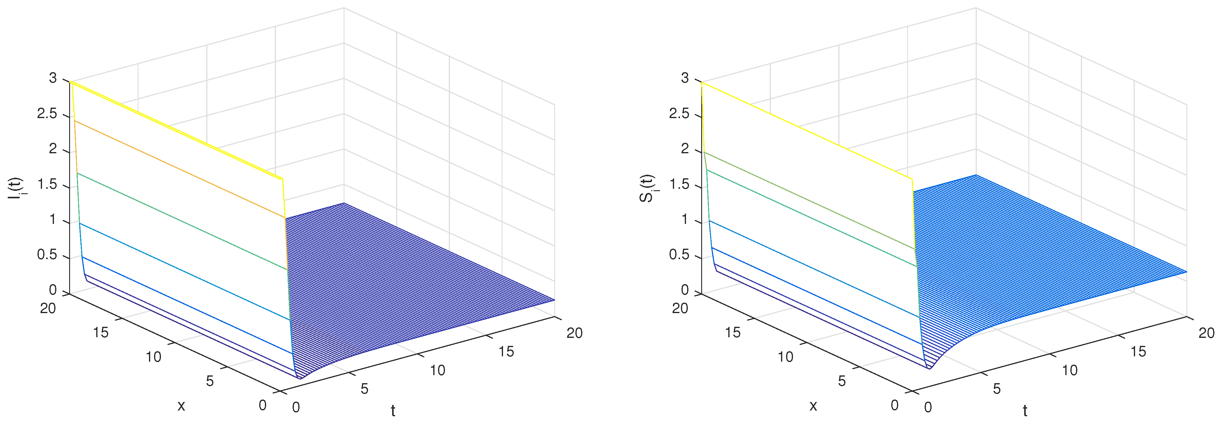
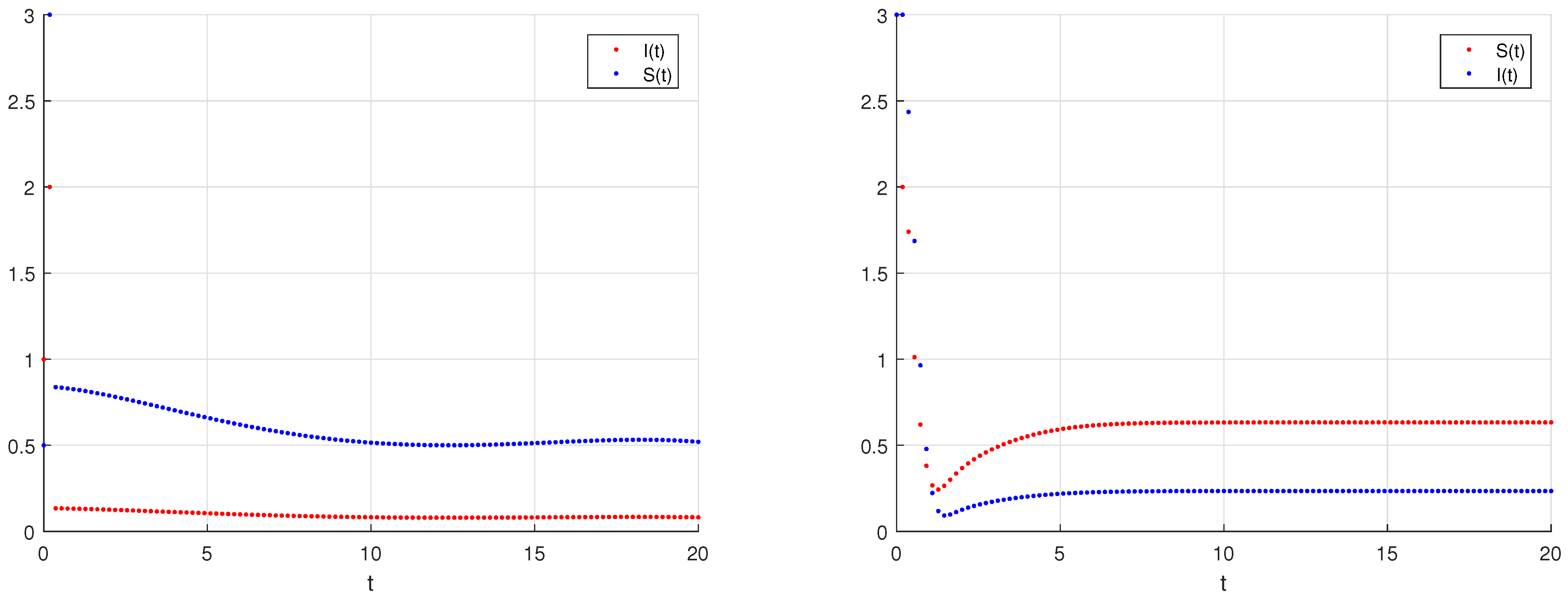
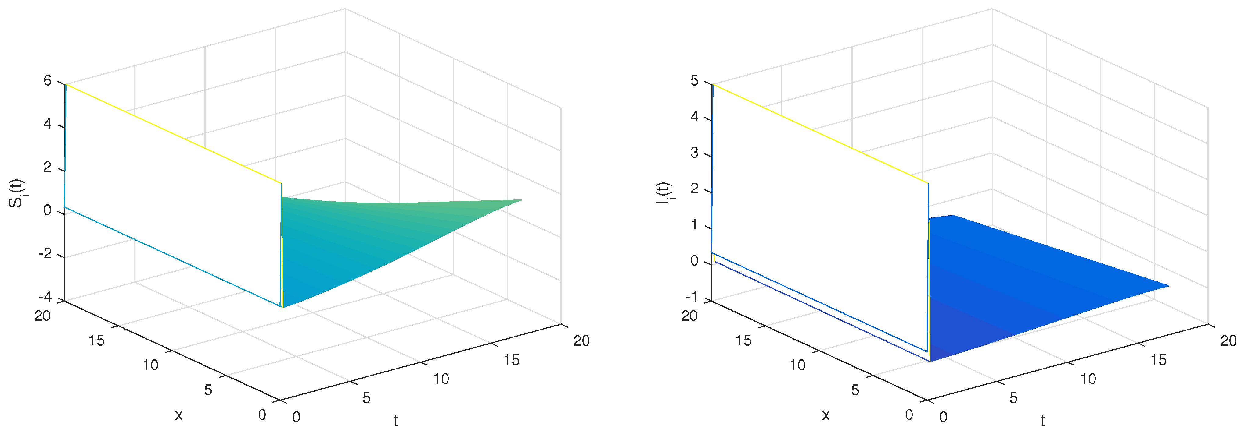
It is easy to see that R 0 stands at 0.6 , a value below the limit of 1. In accordance with the principles outlined in Theorem 6, the disease-free equilibrium point E 0 = ( 0.5 , 0 ) within the framework of System (46) is endowed with global stability, a substantiated assertion illustrated by Figure 1, Figure 2 and Figure 3. Additionally, for the following parameters:
k 1 = 2 , k 2 = 1 , θ = 5 , γ = 1 , ϵ = 2 , ν = 0.2 , σ = 0.3 .
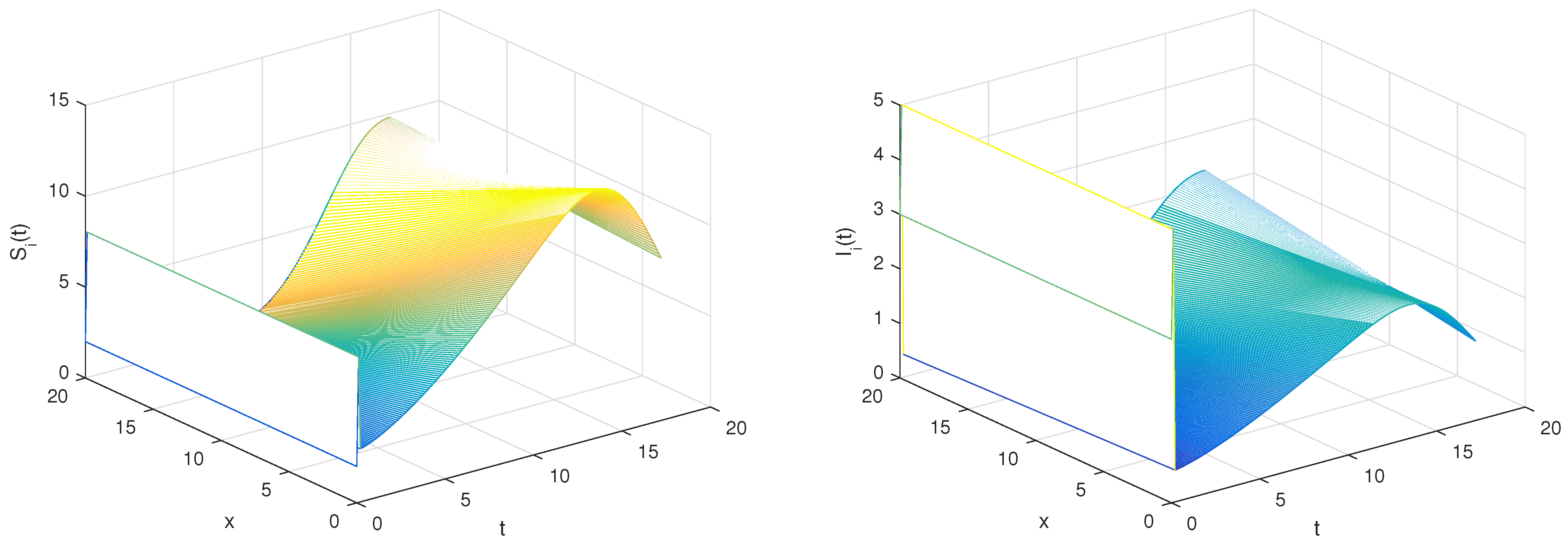
Within System (46), a single equilibrium point denoted as E * prevails. The calculation of R 0 yields a value of 10, surpassing the threshold of 1 as prescribed by Equation (46). It is noteworthy that the endemic equilibrium point E * within System (46), as substantiated by the aforementioned investigation, enjoys global stability, a conclusion supported by the evidence presented in Figure 4 stable.
Example 2.
We use the following incidence rate as an illustration:
ψ ( I ) = I 1 + δ I ,
where δ is a positive parameter measuring the psychological or inhibitory effect. System (9) is expressed as follows:
C Δ t 0 ξ S i ( t ) = k 1 d x 2 Δ 2 S i 1 ( t + ξ ) + θ γ S i ( t + ξ ) I i ( t + ξ ) 1 + δ I i ( t + ξ ) ϵ S i ( t + ξ ) , C Δ t 0 ξ I i ( t ) = k 2 d x 2 Δ 2 I i 1 ( t + ξ ) + γ S i ( t + ξ ) I i ( t + ξ ) 1 + δ I i ( t + ξ ) ( ν + σ ) I i ( t + ξ ) .
and the numerical solution of System (51) is provided by
S i ( n ) = ψ 1 ( x i ) + α Γ ( α ) r = 1 n Γ ( n r + α ) Γ ( n r + 1 ) [ S i + 1 ( ( r 1 ) ) 2 S i ( ( r 1 ) ) + S i 1 ( ( j 1 ) ) d x 2 + θ γ S i ( ( r 1 ) ) I i ( ( r 1 ) ) 1 + δ I i ( ( r 1 ) ) ϵ S i ( ( r 1 ) ) ] , I i ( n ) = ψ 2 ( x i ) + α Γ ( α ) r = 1 n Γ ( n r + α ) Γ ( n r + 1 ) [ I i + 1 ( ( r 1 ) ) 2 I i ( ( r 1 ) ) + I i 1 ( ( r 1 ) ) k 2 + γ S i ( ( r 1 ) ) I i ( ( r 1 ) ) 1 + δ I i ( ( r 1 ) ) ( ν + σ ) I i ( ( r 1 ) ) ] , 1 i m , n > 0 .
We supply the system with the following settings:
k 1 = 3 , k 2 = 2 , θ = 1 2 , γ = 1 2 , ϵ = 2 7 , ν = 0.2 , σ = 0.7 .
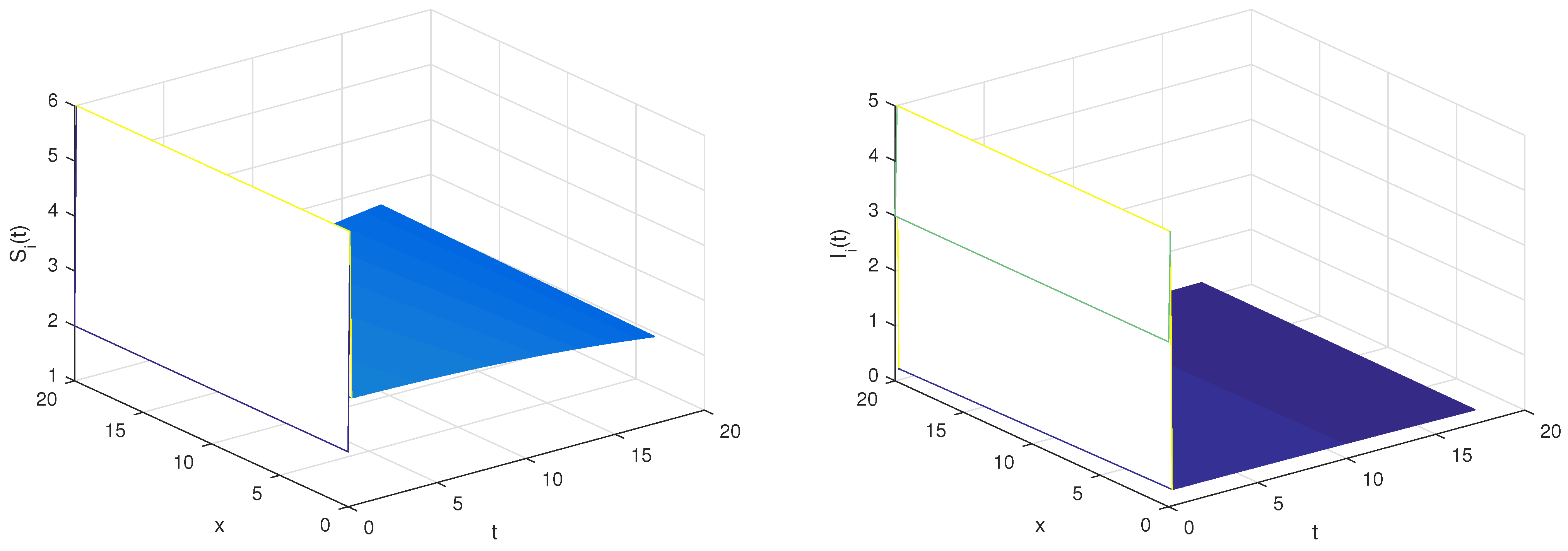
Computing R 0 as 0.9 , which is less than 1, is a straightforward task. It is noteworthy that the disease-free equilibrium point E 0 = ( 1 , 0 ) of System (51) exhibits global stability, as evidenced in Figure 5 and Figure 6.

7. Conclusions

This study explores the discrete version of the fractional reaction–diffusion epidemic system featuring a generalized incidence rate. Notably, when the fractional order approaches unity, the system naturally transitions into its discrete form through the use of the forward difference scheme. The core of our investigation lies in the analysis of the asymptotic stability of this discretized system. The conclusions drawn are in line with those of the corresponding continuous system, suggesting a compelling alignment between discrete and continuous dynamics. This insight emphasizes the capacity of a discrete system, precisely formulated using an L1 finite difference scheme and a second-order central difference scheme, to acquire key characteristics from the continuous version, including positivity, boundedness, and global stability of equilibrium points. Enhancing this theoretical investigation, our numerical simulations validate the proposed approach’s efficiency and applicability. These simulations not only validate the feasibility of our methodology but also highlight its practical effectiveness in capturing system dynamics.

Author Contributions

Conceptualization, H.A.-T.; Methodology, A.A.-H.; Software, M.A.; Validation, O.A.; Formal analysis, M.S.A.; Investigation, A.H.; Writing—original draft, A.H.; Writing—review & editing, A.O.; Visualization, G.M.G. and N.A.-A.; Supervision, A.O. All authors have read and agreed to the published version of the manuscript.

Funding

This research received no external funding.

Institutional Review Board Statement

Not applicable.

Informed Consent Statement

Not applicable.

Data Availability Statement

Not applicable.

Conflicts of Interest

The authors declare no conflict of interest.

References

  1. El-Saka, H.A.A. The fractional-order SIS epidemic model with variable population size. J. Egypt. Math. Soc. 2014, 22, 50–54. [Google Scholar] [CrossRef]
  2. Vargas-De-León, C. Volterra-type Lyapunov functions for fractional-order epidemic systems. Commun. Nonlinear Sci. Numer. Simul. 2015, 24, 75–85. [Google Scholar] [CrossRef]
  3. Ahmed, E.; Elgazzar, A.S. On fractional order differential equations model for nonlocal epidemics. Phys. A Stat. Mech. Its Appl. 2007, 379, 607–614. [Google Scholar] [CrossRef]
  4. Rihan, F.A.; Al-Mdallal, Q.M.; AlSakaji, H.J.; Hashish, A. A fractional-order epidemic model with time-delay and nonlinear incidence rate. Chaos Solitons Fractals 2019, 126, 97–105. [Google Scholar] [CrossRef]
  5. He, Z.Y.; Abbes, A.; Jahanshahi, H.; Alotaibi, N.D.; Wang, Y. Fractional-order discrete-time SIR epidemic model with vaccination: Chaos and complexity. Mathematics 2022, 10, 165. [Google Scholar] [CrossRef]
  6. Can, N.H.; Nikan, O.; Rasoulizadeh, M.N.; Jafari, H.; Gasimov, Y.S. Numerical computation of the time non-linear fractional generalized equal width model arising in shallow water channel. Therm. Sci. 2020, 24, 49–58. [Google Scholar] [CrossRef]
  7. Asaduzzaman, M.; Kilicman, A.; Ali, M.Z. Presence and diversity of positive solutions for a Caputo-type fractional order nonlinear differential equation with an advanced argument. J. Math. Comput. Sci 2021, 23, 230–244. [Google Scholar] [CrossRef]
  8. AlAhmad, R.; AlAhmad, Q.; Abdelhadi, A. Solution of fractional autonomous ordinary differential equations. J. Math. Comput. Sci. 2022, 27, 59–64. [Google Scholar] [CrossRef]
  9. Henry, B.I.; Wearne, S.L. Fractional reaction–diffusion. Phys. A Stat. Mech. Its Appl. 2000, 276, 448–455. [Google Scholar] [CrossRef]
  10. Seki, K.; Wojcik, M.; Tachiya, M. Fractional reaction-diffusion equation. J. Chem. Phys. 2003, 119, 2165–2170. [Google Scholar] [CrossRef]
  11. Gafiychuk, V.; Datsko, B.; Meleshko, V. Mathematical modeling of time fractional reaction–diffusion systems. J. Comput. Appl. Math. 2008, 220, 215–225. [Google Scholar] [CrossRef]
  12. Owolabi, K.M.; Atangana, A.; Akgul, A. Modelling and analysis of fractal-fractional partial differential equations: Application to reaction-diffusion model. Alex. Eng. J. 2020, 59, 2477–2490. [Google Scholar] [CrossRef]
  13. Akram, T.; Abbas, M.; Ali, A. A numerical study on time fractional Fisher equation using an extended cubic B-spline approximation. J. Math. Comput. Sci. 2021, 22, 85–96. [Google Scholar] [CrossRef]
  14. Zhou, P.; Ma, J.; Tang, J. Clarify the physical process for fractional dynamical systems. Nonlinear Dyn. 2020, 100, 2353–2364. [Google Scholar] [CrossRef]
  15. Angstmann, C.N.; Henry, B.I.; McGann, A.V. A fractional-order infectivity SIR model. Phys. A Stat. Mech. Appl. 2016, 452, 86–93. [Google Scholar] [CrossRef]
  16. Hethcote, H.W. The mathematics of infectious diseases. SIAM Rev. 2000, 42, 599–653. [Google Scholar] [CrossRef]
  17. Almeida, R. Analysis of a fractional SEIR model with treatment. Appl. Math. Lett. 2018, 84, 56–62. [Google Scholar] [CrossRef]
  18. Angstmann, C.N.; Donnelly, I.C.; Henry, B.I.; Jacobs, B.A.; Langlands, T.A.M.; Nichols, J.A. From stochastic processes to numerical methods: A new scheme for solving reaction subdiffusion fractional partial differential equations. J. Comput. Phys. 2016, 307, 508–534. [Google Scholar] [CrossRef]
  19. Angstmann, C.N.; Donnelly, I.C.; Henry, B.I.; Nichols, J.A. A discrete time random walk model for anomalous diffusion. J. Comput. Phys. 2015, 293, 53–69. [Google Scholar] [CrossRef]
  20. Angstmann, C.N.; Henry, B.I.; McGann, A.V. A fractional order recovery SIR model from a stochastic process. Bull. Math. Biol. 2016, 78, 468–499. [Google Scholar] [CrossRef]
  21. Dababneh, A.; Djenina, N.; Ouannas, A.; Grassi, G.; Batiha, I.M.; Jebril, I.H. A new incommensurate fractional-order discrete COVID-19 model with vaccinated individuals compartment. Fractal Fract. 2022, 6, 456. [Google Scholar] [CrossRef]
  22. Saadeh, R.; Abbes, A.; Al-Husban, A.; Ouannas, A.; Grassi, G. The Fractional Discrete Predator–Prey Model: Chaos, Control and Synchronization. Fractal Fract. 2023, 7, 120. [Google Scholar] [CrossRef]
  23. Yi, N.; Liu, P.; Zhang, Q. Bifurcations analysis and tracking control of an epidemic model with nonlinear incidence rate. Appl. Math. Model. 2012, 36, 1678–1693. [Google Scholar] [CrossRef]
  24. Chen-Charpentier, B.M.; Dimitrov, D.T.; Kojouharov, H.V. Numerical simulation of multi-species biofilms in porous media for different kinetics. Math. Comput. Simul. 2009, 79, 1846–1861. [Google Scholar] [CrossRef]
  25. Jang, S.; Elaydi, S. Difference equations from discretization of a continuous epidemic model with immigration of infectives. Math. Fac. Res. 2003, 11, 93–105. [Google Scholar]
  26. Sekiguchi, M.; Ishiwata, E. Global dynamics of a discretized SIRS epidemic model with time delay. J. Math. Anal. Appl. 2010, 371, 195–202. [Google Scholar] [CrossRef]
  27. Almatroud, O.A.; Hioual, A.; Ouannas, A.; Grassi, G. On Fractional-Order Discrete-Time Reaction Diffusion Systems. Mathematics 2023, 11, 2447. [Google Scholar] [CrossRef]
  28. Wu, G.C.; Baleanu, D.; Zeng, S.D.; Deng, Z.G. Discrete fractional diffusion equation. Nonlinear Dyn. 2015, 80, 281–286. [Google Scholar] [CrossRef]
  29. Wu, G.C.; Baleanu, D.; Xie, H.P.; Zeng, S.D. Discrete fractional diffusion equation of chaotic order. Int. J. Bifurc. Chaos 2016, 26, 1650013. [Google Scholar] [CrossRef]
  30. Lu, Z.; Yu, Y.; Xu, W.; Ren, G.; Meng, X. Global dynamics for a class of discrete fractional epidemic model with reaction-diffusion. arXiv 2022, arXiv:2208.06548. [Google Scholar]
  31. Abu Falahah, I.; Hioual, A.; Al-Qadri, M.O.; AL-Khassawneh, Y.A.; Al-Husban, A.; Hamadneh, T.; Ouannas, A. Synchronization of Fractional Partial Difference Equations via Linear Methods. Axioms 2023, 12, 728. [Google Scholar] [CrossRef]
  32. Hamadneh, T.; Hioual, A.; Alsayyed, O.; AL-Khassawneh, Y.A.; Al-Husban, A.; Ouannas, A. Local Stability, Global Stability, and Simulations in a Fractional Discrete Glycolysis Reaction–Diffusion Model. Fractal Fract. 2023, 7, 587. [Google Scholar] [CrossRef]
  33. Hamadneh, T.; Hioual, A.; Alsayyed, O.; Al-Khassawneh, Y.A.; Al-Husban, A.; Ouannas, A. The FitzHugh–Nagumo Model Described by Fractional Difference Equations: Stability and Numerical Simulation. Axioms 2023, 12, 806. [Google Scholar] [CrossRef]
  34. Lu, Z.; Yu, Y.; Ren, G.; Xu, C.; Meng, X. Global dynamics for a class of reaction–diffusion multigroup SIR epidemic models with time fractional-order derivatives. Nonlinear Anal. Model. Control. 2022, 27, 142–162. [Google Scholar] [CrossRef]
  35. Kelley, W.G.; Peterson, A.C. Difference Equations: An Introduction with Applications; Academic Press: Cambridge, MA, USA, 2001. [Google Scholar]
  36. Sharkovsky, A.N.; Maistrenko, Y.L.T.; Romanenko, E.Y. Difference Equations and Their Applications; Springer Science & Business Media: Berlin/Heidelberg, Germany, 2012; Volume 250. [Google Scholar]
  37. Baleanu, D.; Wu, G.C.; Bai, Y.R.; Chen, F.L. Stability analysis of Caputo–like discrete fractional systems. Commun. Nonlinear Sci. Numer. Simul. 2017, 48, 520–530. [Google Scholar] [CrossRef]
  38. Hioual, A.; Ouannas, A.; Oussaeif, T.E.; Grassi, G.; Batiha, I.M.; Momani, S. On variable-order fractional discrete neural networks: Solvability and stability. Fractal Fract. 2022, 6, 119. [Google Scholar] [CrossRef]
  39. Van den Driessche, P.; Watmough, J. Reproduction numbers and sub-threshold endemic equilibria for compartmental models of disease transmission. Math. Biosci. 2002, 180, 29–48. [Google Scholar] [CrossRef]
  40. Čermák, J.; Nechvátal, L. On a problem of linearized stability for fractional difference equations. Nonlinear Dyn. 2021, 104, 1253–1267. [Google Scholar] [CrossRef]
  41. Xu, L.; Zhao, L.J.; Chang, Z.X.; Feng, J.T.; Zhang, G. Turing instability and pattern formation in a semi-discrete Brusselator model. Mod. Phys. Lett. B 2013, 27, 1350006. [Google Scholar] [CrossRef]
  42. Franco-Perez, L.; Fernandez-Anaya, G.; Quezada-Téllez, L.A. On stability of nonlinear nonautonomous discrete fractional Caputo systems. J. Math. Anal. Appl. 2020, 487, 124021. [Google Scholar] [CrossRef]
  43. Elaydi, S. An Introduction to Difference Equations; Springer: San Antonio, TX, USA, 2015. [Google Scholar]
  44. Anakira, N.; Hioual, A.; Ouannas, A.; Oussaeif, T.E.; Batiha, I.M. Global Asymptotic Stability for Discrete-Time SEI Reaction-Diffusion Model. In International Conference on Mathematics and Computations; Springer Nature: Singapore, 2022; pp. 345–357. [Google Scholar]
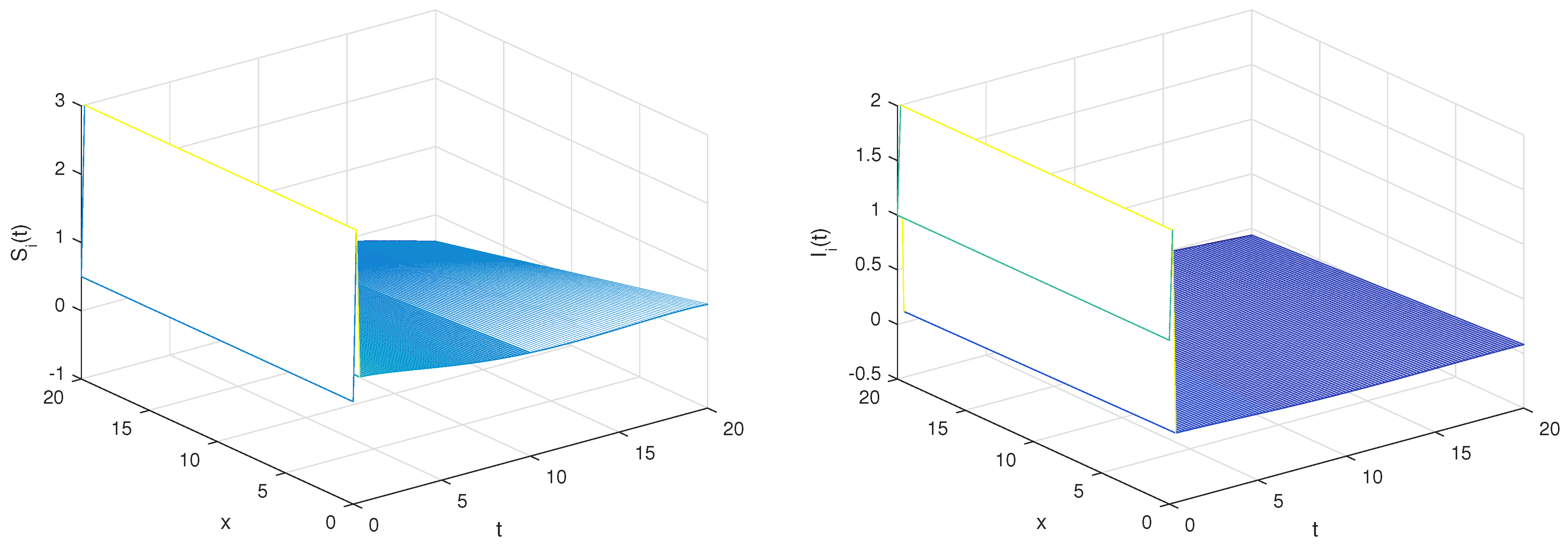
Figure 1. Dynamic behaviors of S i ( t ) and I i ( t ) for N = 110 and the periodic boundary condition ( S 0 , I 0 ) = ( 3 , 2 ) and the fractional order α = 0.8 .
Fractalfract 07 00729 g001
Figure 2. Dynamic behaviors of S i ( t ) and I i ( t ) for N = 110 and the periodic boundary condition ( S 0 , I 0 ) = ( 3 , 3 ) and the fractional order α = 0.5 .
Fractalfract 07 00729 g002
Figure 3. State trajectories of S i ( t ) and I _ i ( t ) for N = 110 .
Fractalfract 07 00729 g003
Figure 4. Dynamic behaviors of S i ( t ) and I i ( t ) for N = 200 and the periodic boundary condition ( S 0 , I 0 ) = ( 6 , 5 ) and the fractional order α = 0.1 .
Fractalfract 07 00729 g004
Figure 5. Dynamic behaviors of S i ( t ) and I i ( t ) for N = 200 and the periodic boundary condition ( S 0 , I 0 ) = ( 6 , 5 ) and the fractional order α = 0.7 .
Fractalfract 07 00729 g005
Figure 6. Dynamic behaviors of S i ( t ) and I i ( t ) for N = 200 and the periodic boundary condition ( S 0 , I 0 ) = ( 6 , 5 ) and the fractional order α = 0.2 .
Fractalfract 07 00729 g006
Disclaimer/Publisher’s Note: The statements, opinions and data contained in all publications are solely those of the individual author(s) and contributor(s) and not of MDPI and/or the editor(s). MDPI and/or the editor(s) disclaim responsibility for any injury to people or property resulting from any ideas, methods, instructions or products referred to in the content.