A Joint Multifractal Approach to Solar Wind Turbulence

Abstract

Previous studies have shown that solar wind, a plasma medium with turbulent dynamics, exhibits anomalous scaling features, i.e., intermittency, in the inertial domain. This intermittent nature has primarily been investigated through the study of the scaling features of the structure functions of single quantities. We use a novel approach based on joint multifractal analysis in this study to simultaneously investigate the scaling characteristics of both the magnetic field and the plasma velocity in solar wind turbulence. Specifically, we focus on the joint multifractal behavior of magnetic and velocity field fluctuations in both fast and slow solar wind streams observed by the ESA-Ulysses satellite, with the goal of identifying any differences in their joint multifractal characteristics.

1. Introduction

Space plasmas display non-trivial, non-linear, and complex dynamics, which take the form of multiscale features, chaos, and turbulence in many astrophysical and space environments. Understanding and studying this emergent complexity necessitate the application of methods and approaches developed in other research areas, especially those derived from dynamical systems physics.

In this sense, the heliosphere, which includes solar wind and planetary environments, provides a natural laboratory for studying how the complexity and complex dynamical features emerge in space plasmas. Within these plasma environments, phenomena like turbulence and chaos play critical roles in plasma diffusion, transport, energization, and particle acceleration. The investigation of turbulence in space plasma media, especially in solar wind, has a rich history that dates back to the late 1960s when Coleman [1] made significant strides in this field. Utilizing magnetic and plasma observations from the Mariner 2 spacecraft, he presented the first evidence of the turbulence spectrum of solar wind fluctuations spanning over several frequency decades. This groundbreaking discovery laid the foundation for extensive research aimed at gaining a deeper understanding of the turbulent nature and dynamics of solar wind. Furthermore, these findings are consistent with the inherent characteristics of solar wind as a plasma with remarkably low viscosity and resistivity, resulting in high kinetic and magnetic Reynolds numbers in the magnetohydrodynamic (MHD) equations. These high Reynolds numbers indicate the dominance of non-linear terms over dissipative terms, implying that significant turbulent effects are likely in solar wind. Over the years, researchers have made significant progress in understanding the turbulent nature of solar wind [2,3]. However, in the 1970s and 1980s, when in situ observations were mainly carried out in the ecliptic plane, a significant advance in our comprehension of solar wind turbulence took place. During this period, spacecraft observations were limited to a narrow latitudinal range around the solar equator, offering only a bidimensional (2D) perspective of the heliosphere. Fortunately, this limitation was overcome in the 1990s with the launch of the Ulysses spacecraft. Ulysses provided a unique opportunity to extend investigations to the high-latitude regions of the heliosphere, providing crucial insights into how turbulence evolves in the polar regions. Researchers have primarily focused on studying the spectral and scaling features of solar wind turbulence, examining how they evolve with the radial distance from the Sun within the heliosphere, and comparing these observed features to theoretical predictions from magnetohydrodynamic (MHD) approaches [3,4].

It is now well established in the context of solar wind research that turbulence in solar wind exhibits the property of intermittency. Intermittency is a common feature observed in many complex physical systems in nature, indicating that fluctuations are not strictly self-similar and that energy is not distributed uniformly in space across all scales. This phenomenon challenges the classical Kolmogorov 5/3 law of turbulence, which assumes a globally scale-invariant and homogeneous behavior (Kolmogorov, 1941). However, Obukhov (1962) later proposed that the energy transfer rate from larger to smaller structures, initially assumed to be scale-independent by Kolmogorov, can actually fluctuate over space and time. This variability in energy dissipation and transfer rates forms the foundation of intermittency. In the case of solar wind turbulence, intermittency is manifested through fluctuations of energy at different scales. Early investigations into solar wind’s fluctuations date back to the 1990s, primarily focusing on investigating the anomalous scaling features of structure functions in the inertial range [5,6,7,8,9]. These studies, in particular, revealed the presence of anomalous scaling laws for structure functions of solar wind velocity fluctuations at various scales, encompassing both the inertial and injection ranges of scales. Additionally, studies explored the multifractal character of measures related to magnetic and velocity field fluctuations [10,11], as well as the features of probability density functions (PDFs) of magnetic and velocity field increments in the inertial range [12,13]. Intermittency in solar wind at fluid MHD scales has been attributed primarily to coherent structures of solar or local origin that are advected by the wind. These structures, which have been identified as primarily parallel shocks, slow mode shocks, or tangential discontinuities/current sheets, appear to play an important role in the generation of intermittent features in solar wind [14].

All previous studies have focused on analyzing single quantities (velocity field, magnetic field and so on), without considering the potential correlations between the singular character of different quantities. Investigating the cross-singularity spectra associated with two distinct measurable quantities using joint multifractal analysis introduced by Meneveau et al. [15] could be a promising step forward in characterizing the intermittent nature of solar wind turbulence.

Indeed, this method extends the traditional multifractal formalism to multiple variables, allowing for the investigation of simultaneous cascading processes [15,16].

In this study, we utilize joint multifractal analysis to examine the magnetic and velocity fields in two distinct solar wind conditions: high-latitude fast solar wind and low-latitude slow solar wind, as observed by the Ulysses mission. Indeed, one of the most significant characteristics of solar wind is its bimodal nature, as it can be classified into two main types: fast and slow solar wind [3]. These two types of solar wind exhibit distinct properties and have different origins. Fast solar wind is typically observed at high latitudes of the Sun, near its poles. It originates from coronal holes, which are regions in the Sun’s corona with lower magnetic field intensity. These coronal holes allow high-speed plasma streams to escape more easily into space. Fast solar wind is characterized by higher speeds, reaching up to 700 km per second at 1 astronomical unit (AU) from the Sun, and lower densities compared to slow solar wind. On the other hand, slow solar wind is mostly observed at low latitudes of the Sun, near the equator. It comes from regions with closed magnetic field lines, known as the streamer belt. Slow solar wind flows along these magnetic field lines and is released into the interplanetary space. When compared to fast solar wind, it has lower speeds, around 400 km per second at 1 AU, and higher densities.

The goal of this study is to investigate change in the correlation between the singularity spectra of these two solar wind conditions within the MHD inertial range.

2. Method: Joint Multifractal Analysis

The multifractal formalism is undoubtedly one of the most powerful statistical techniques for investigating the scaling and self-similarity properties of mathematical and physical objects and signals. In detail, a multifractal measure can be conceptualized from a broad mathematical perspective as a fractal measure defined on a fractal domain or set, where multifractality arises due to the interplay between two families of singularities. The aim of the multifractal formalism is to describe the self-similarity of a fractal object by using a hierarchy of generalized dimensions, denoted as $D_q$ or Renyi’s dimensions. Additionally, it involves the multifractal singularity spectrum, $f\left(\alpha \right)$, which characterizes the dimensions associated with the set of singularities of strength $\alpha$ [17].

Joint multifractal analysis represents a natural multidimensional extension of the multifractal formalism. It was originally introduced by Meneveau et al. [15] in the context of high-Reynolds-number turbulence to quantify the correlation between intermittent fields, specifically, the coexisting distributions of such fields. Over time, this method has found applications in various research fields, including financial markets’ studies, investigations related to rainfall, agronomy studies, and more [16,18,19,20]. The versatility of this approach has enabled its application in diverse domains, making it a valuable tool for exploring correlations in intermittent phenomena.

Despite the original method proposed by Meneveau et al. [15], which was based on the traditional partition functions approach, alternative methods have been developed over time to explore the joint multifractality of coupled measures. Some of these alternative methods include joint structure–function analysis, multifractal wavelet coherence analysis, and others (see Ref. Jiang et al. [16] for more details). In this study, we focus on the traditional method proposed by Meneveau et al. [15], which is based on partition function analysis. This method assumes that the measures defined on the velocity and magnetic field coexist in the same sample space domain.

Consider two distinct experimental measures, ${\varphi }_1$ and ${\varphi }_2$, defined over the same domain $\mathcal{S}$. Let $s_i(𝓁)$ be a non-overlapping partition of order N of the domain $\mathcal{S}$, consisting of elementary boxes of dimension ℓ, i.e., ${\sum }_{i=1}^N{s}_i(𝓁)\equiv \mathcal{S}$. For each box, consider the fractions ${ϵ}_{i,1}(𝓁)$ and ${ϵ}_{i,2}(𝓁)$ of the measures associated with each box, and define two new measures ${\mu }_{i,j}(p,𝓁)$ (where $j=1,2$) of moment order p as follows:

$${\mu }_{i,j}(p,𝓁)={\left[{ϵ}_{i,j}(𝓁)\right]}^p,\forall j=1\mathrm{or}2.$$

(1)

In the case of the standard multifractal analysis, we now compute the scaling features of the partition function associated with the defined measure, i.e.,

$$\chi (𝓁,p)=\sum _i{\mu }_i(p,𝓁)=\sum _i{\left[{ϵ}_i(𝓁)\right]}^p\simeq {𝓁}^{\tau \left(p\right)},$$

(2)

where $\tau \left(p\right)$ is the scaling exponent associated with the moment order p. From this equation, by simply applying a Legendre transform, it is possible to compute the corresponding multifractal spectrum $f\left(\alpha \right)$, i.e.,

$$f\left(\alpha \right)=p\alpha \left(p\right)-\tau \left(p\right),$$

(3)

where $\alpha \left(p\right)=d\tau \left(p\right)/dp$.

Analogously, in the case of the joint multifractal analysis, it is possible to introduce a joint-partition function $\chi (𝓁;p,q)$ as

$$\chi (𝓁;p,q)=\sum _i{\mu }_{i,1}(p,𝓁){\mu }_{i,2}(q,𝓁)\equiv \sum _i{\left[{ϵ}_{i,1}(𝓁)\right]}^p{\left[{ϵ}_{i,2}(𝓁)\right]}^q.$$

(4)

In the case of scaling features, the partition function $\chi (𝓁;p,q)$ is expected to scale with the box dimension ℓ according to a power law,

$$\chi (𝓁;p,q)\sim {𝓁}^{\tau (q,p)},$$

(5)

where $\tau (q,p)$ is a joint-scaling exponent analogous to the exponent $\tau \left(q\right)$ of single multifractal analysis.

The knowledge of the joint-scaling exponent $\tau (q,p)$ allows computing the joint-singularity spectrum $f(\alpha ,{\alpha }^{\prime })$ using a double Legendre transform that links the triads $(\tau ,p,q)$ with the corresponding $(f,\alpha ,{\alpha }^{\prime })$, i.e.,

$$\begin{array}{ccc}\hfill \alpha (q,p)& =& \frac{\partial }{\partial q}\tau (q,p),\hfill \end{array}$$

(6)

$$\begin{array}{ccc}\hfill {\alpha }^{\prime }(q,p)& =& \frac{\partial }{\partial p}\tau (q,p),\hfill \end{array}$$

(7)

$$\begin{array}{ccc}\hfill f(\alpha ,{\alpha }^{\prime })& =& q\alpha (q,p)+p{\alpha }^{\prime }(q,p)-\tau (q,p).\hfill \end{array}$$

(8)

It is important to remark that this kind of analysis is complementary to the usual structure–function analysis, being a link between the observed joint-scaling exponent $\tau (q,p)$ and the structure–function ones. For an extended discussion on this point, we invite the readers to refer to Meneveau et al. [15] and to Benzi and Toschi [21].

3. Data

We use data from the ESA-Ulysses mission in this study, focusing on magnetic and velocity field measurements in the heliosphere. More specifically, we look at two distinct time periods: a high-latitude fast solar wind period from 1 July 1995 to 31 December 1995, and a low-latitude slow solar wind period from 1 September 1997 to 28 February 1998. These time periods have also been previously examined in some other works, including those by Bavassano et al. [22,23], and Consolini et al. [24]. Data come from the NASA-CDAWeb service of the NSSDC Data Center (accessed on 3 March 2023) and refer to 1 min magnetic field measurements and 4 ÷ 8 min plasma velocity measurements.

Table 1. Average features of the two selected time periods. Latitude is in the Solar Ecliptic Coordinate System. # 1 and # 2 refer to the fast period and the slow period, respectively. $\langle c_A\rangle$ and $\langle c_{MS}\rangle$ are the average Alfvén and fast magnetosonic velocities, respectively.

	R	${\mathit{Lat}}_{\left[\mathbf{SE}\right]}$	$\langle \mathit{v}\rangle$	$\langle \mathit{B}\rangle$	${\mathit{n}}_{\mathit{RMS}}$	$\langle {\mathit{c}}_{\mathit{A}}\rangle$	$\langle {\mathit{c}}_{\mathit{MS}}\rangle$	$\langle \mathit{\beta }\rangle$
	(au)	(deg)	(km/s)	(nT)	(cm${}^{-\mathbf{3}}$)	(km/s)	(km/s)
# 1	$[2.44\pm 0.37]$	$[72\pm 6]$	$[780\pm 20]$	$[1.21\pm 0.35]$	$0.44$	40	50	$1.5$
# 2	$[5.34\pm 0.05]$	$[7.8\pm 2.6]$	$[368\pm 23]$	$[0.68\pm 0.39]$	$0.39$	24	31	$0.5$

provides the key information for the two selected time periods including also the Alfvén velocity $c_A$ and the fast magnetosonic velocity, $c_{MS}=\sqrt{c_A^2+c_s^2}$, where $c_s$ is the sound velocity, and the ion plasma beta $\beta$.

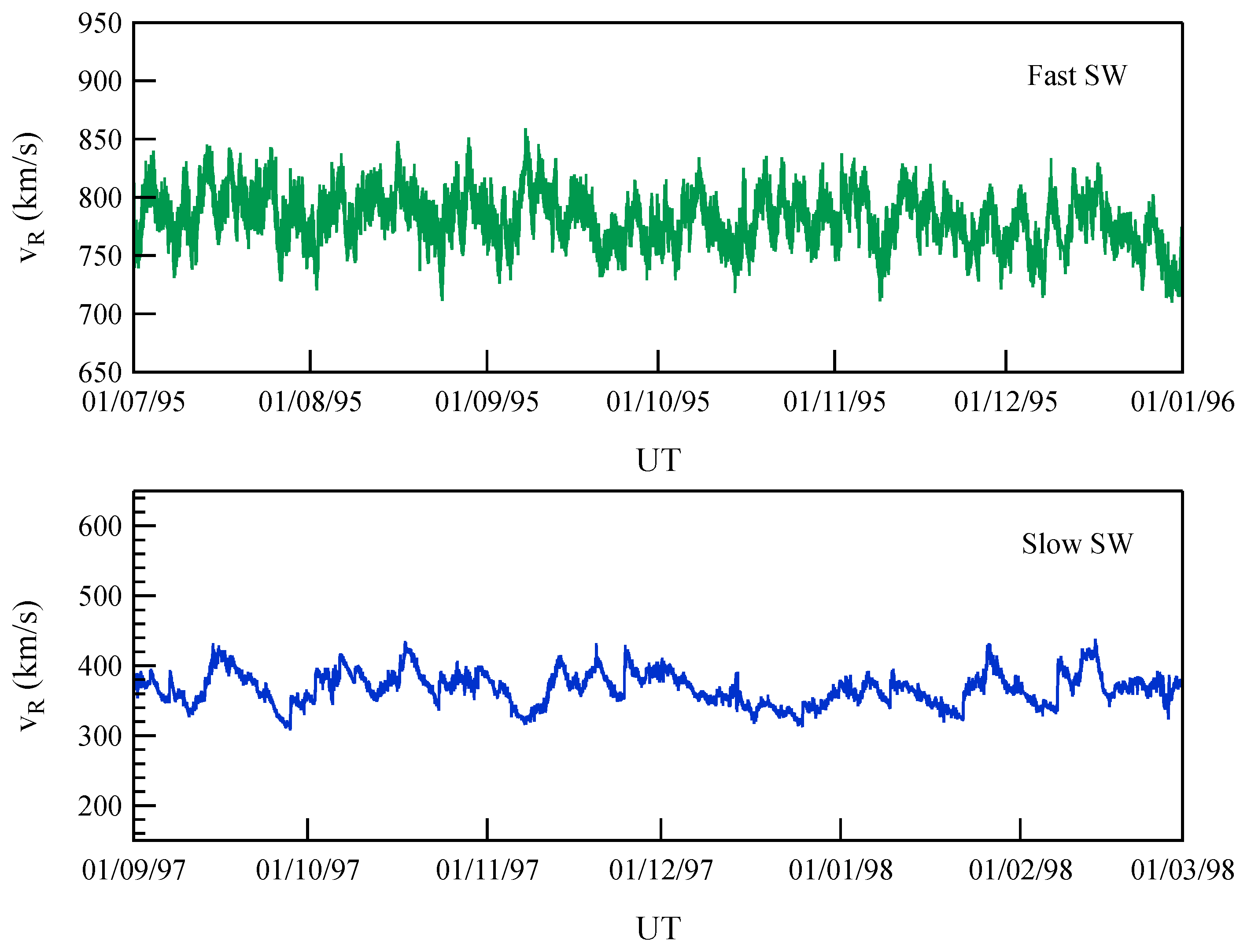
The plots in Figure 1 show the radial velocity $v_R$ for the two time periods chosen, indicating that they correspond to quasi-stationary solar wind conditions. The data are represented in the radial–transverse–normal (RTN) reference frame, with a resolution of 4 min (data relative to magnetic field measurements have been downsampled, whereas data relative to velocity field measurements have been interpolated to achieve a resolution of 4 min). The datasets contain over 64,000 data points, allowing us to investigate moments in the range $q\in [-4,4]$. For our analysis, we focus on the two components perpendicular to the radial direction, namely the transverse (T) and normal (N) components.

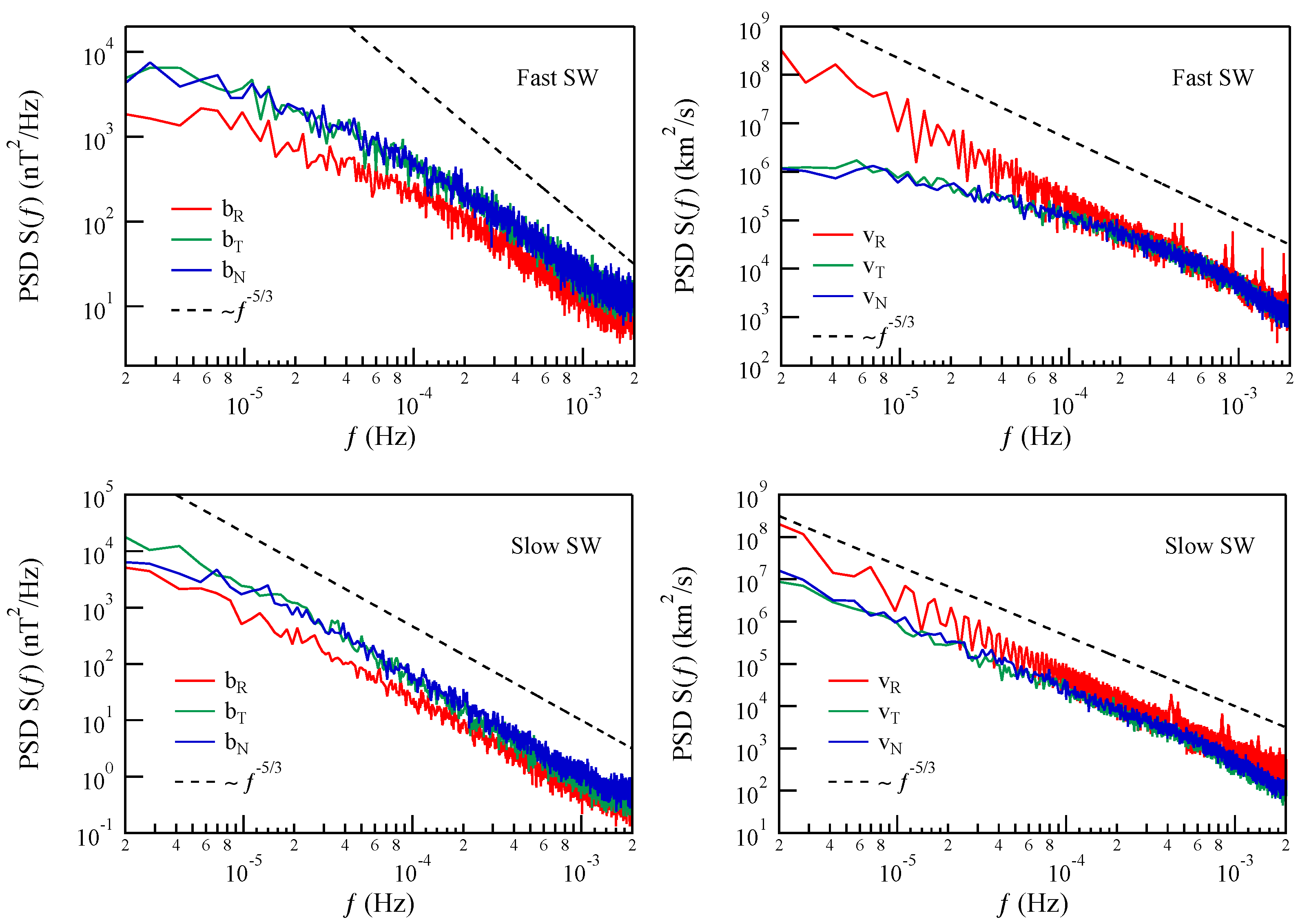
Figure 2 illustrates the power spectral densities of the magnetic and velocity fields along the three directions during the two selected time periods. In more detail, the top section of the figure exhibits two panels, displaying the power spectral densities obtained for the magnetic field (left panel) and the velocity field (right panel) during the fast solar wind period. Conversely, the bottom panels pertain to the analysis conducted for the slow solar wind period, with the left panels representing the power spectral densities of the magnetic field and the right panels depicting those of the velocity field. All the spectral densities exhibit a quasi −5/3 spectral interval, which is consistent with previous studies [see Ref. [3]]. However, the range of scales where the −5/3 spectral interval is present is wider in the slow solar wind period than in the fast solar wind period. This difference might be attributed to a distinct turbulence aging between the two solar wind types, indicating that turbulence is more developed in the slow solar wind period than in the fast one. Another possibility is that they originate from different solar regions, namely coronal holes and closed magnetic field regions. We would like to emphasize that to make a meaningful comparison with theoretical predictions, it is necessary to consider spectra in the Fourier $k–$space. However, since solar wind is supersonic and super-Alfvénic, we can reasonably assume that Taylor’s hypothesis holds, i.e., $f=v_{sw}k$, where $v_{sw}$ is solar wind velocity. Another crucial aspect that becomes apparent from the spectral characteristics is the sudden decrease in power at frequencies greater than ${10}^{-3}$ Hz in the velocity spectra. This decline might be attributed to instrumental limitations. As a result, we focus our joint multifractal analysis on temporal scales longer than 10 min. Moreover, in accordance with Elsasser’s equation for MHD, it is preferable to use the magnetic field (b) in Alfvén units rather than directly considering it in nanotesla (nT), i.e.,

$$\mathbf{b}\to {\mathbf{b}}^A=\frac{\mathbf{b}}{\sqrt{4\pi \rho }},$$

(9)

where $\rho$ is the plasma density. Here, we perform the analysis of the joint multifractal features by using as dynamical variables the magnetic field in Alfvén units and the velocity field.

4. Analysis and Results

The first step necessary to perform joint multifractal analysis requires defining a proper set of measures ${\mu }_i$ over the data set. Among the different measures that can be used to investigate multifractality over data samples, we opt for a measure related to the energy dissipation (transfer) rate $ϵ$ in fluid turbulence, similar to the one introduced by Marsch et al. [11]. In detail, we define the following measures,

$$\begin{array}{ccc}\hfill {\mu }_b\left(t\right)& =& {\left[\delta b_{R,\tau }^A\left(t\right)\right]}^2+{\left[\delta b_{T,\tau }^A\left(t\right)\right]}^2+{\left[\delta b_{N,\tau }^A\left(t\right)\right]}^2,\hfill \end{array}$$

(10)

$$\begin{array}{ccc}\hfill {\mu }_v\left(t\right)& =& {\left[\delta v_{R,\tau }\left(t\right)\right]}^2+{\left[\delta v_{T,\tau }\left(t\right)\right]}^2+{\left[\delta v_{N,\tau }\left(t\right)\right]}^2,\hfill \end{array}$$

(11)

which are related to the total kinetic and magnetic energy dissipation rates, respectively. The expression $\delta x\left(t\right)=x(t+\tau )-x\left(t\right)$, with $\tau =4$ minutes as the data resolution, represents the difference in the values of either the magnetic field or the velocity field at two time points. The term “x” represents the components of the magnetic or velocity field measured along the transverse (T), normal (N), and radial (R) directions. These measures are subsequently renormalized so that

$${\int }_{{\mathrm{\Omega }}_t}{\mu }_i\left(t\right)dt=1,$$

(12)

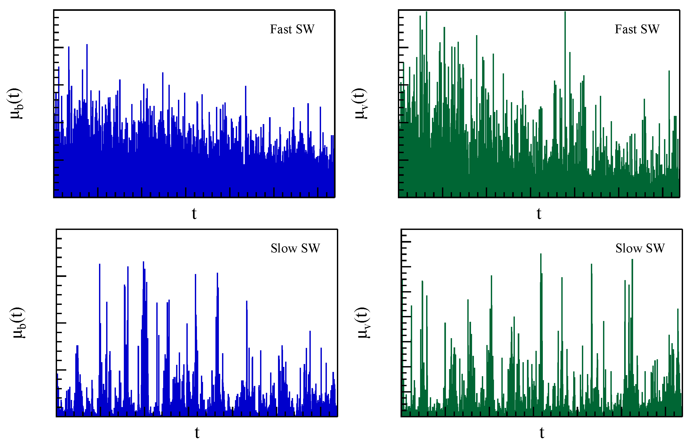
where ${\mathrm{\Omega }}_t$ is the selected time interval. Figure 3 displays the renormalized measures obtained by applying Equations (10) and (11) for fast and slow solar wind, respectively. Upon initial examination, it is evident that the measure ${\mu }_{b,v}$ of the slow solar wind exhibits a more intermittent character.

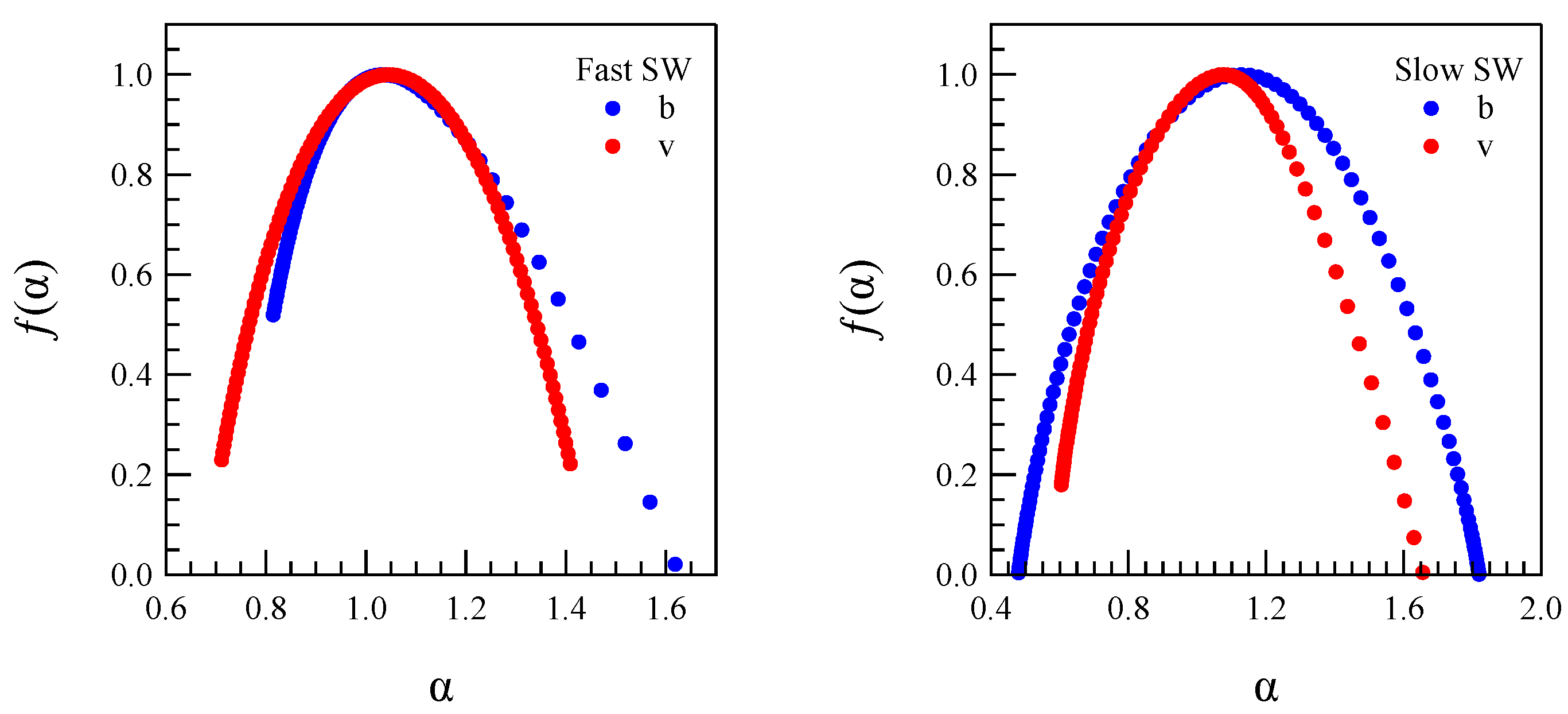
After computing the singularity spectrum, $f\left(\alpha \right)$, of the individual measures based on the definitions provided in Section 2, we present the results for the magnetic field and velocity of the fast and slow solar wind in Figure 4. It can be seen that the magnetic field measure for both fast and slow solar wind has a wider singularity spectrum than the velocity measure, with the slow solar wind having a more pronounced singularity spectrum.

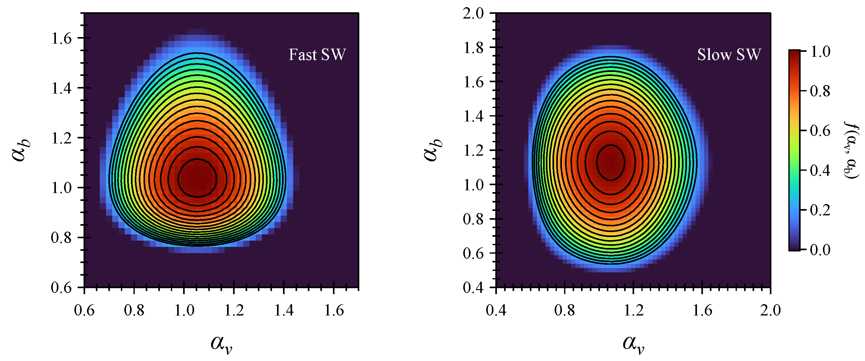
Following the approach proposed by Meneveau et al. [15], we utilize the multifractal singularity spectrum of the individual measures to calculate the expected joint multifractal singularity spectrum, $f({\alpha }_v,{\alpha }_b)$, assuming independent measure distributions. This is given by the following expression,

$$f({\alpha }_v,{\alpha }_b)=f\left({\alpha }_v\right)+f\left({\alpha }_b\right)-d,$$

(13)

where d is the dimension of the domain over which is defined the measures (here, $d=1$).

Figure 5 shows the expected joint-singularity spectra of independent measure distributions.

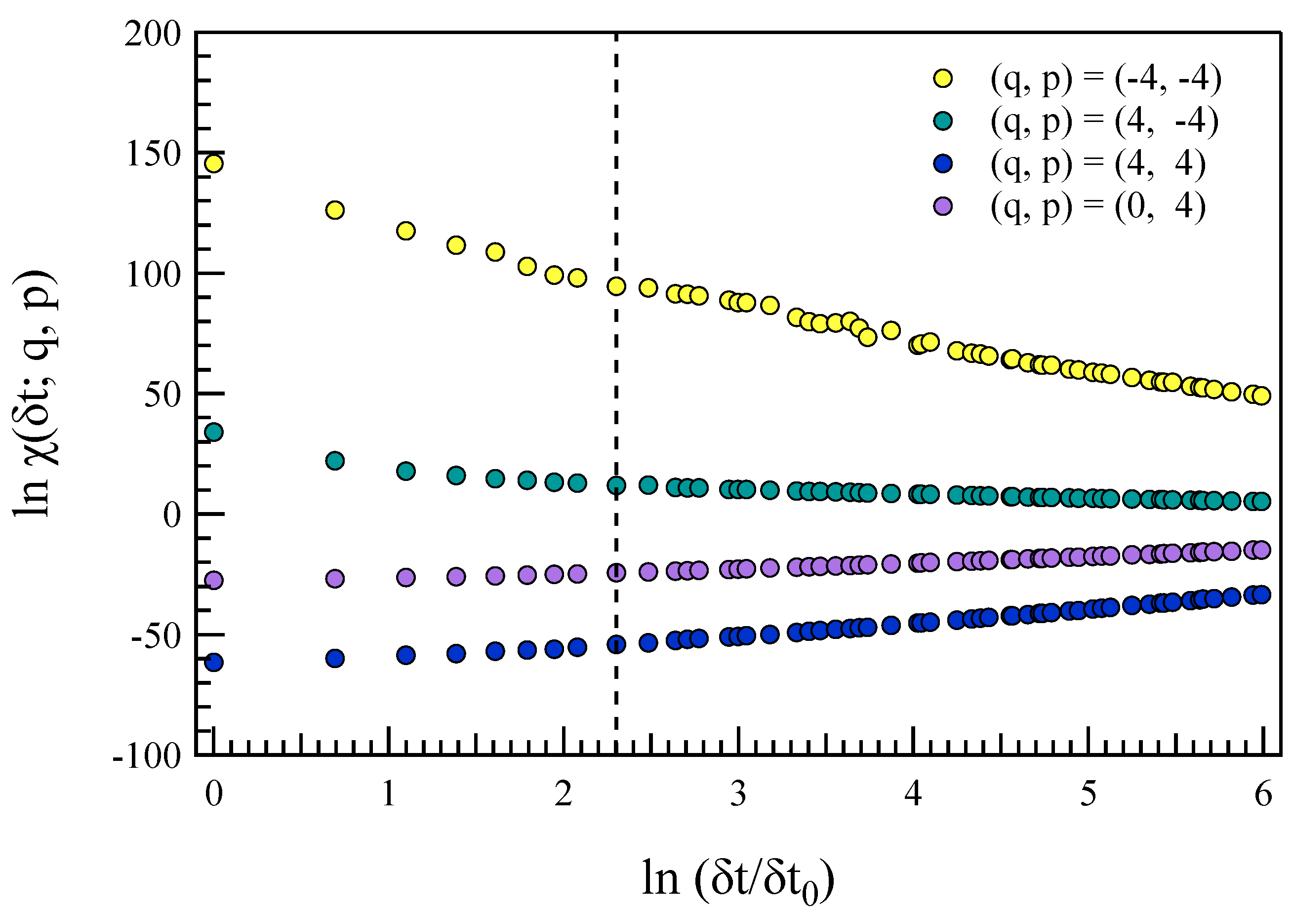
Let us now compute the joint-partition function $\chi (\delta t;q,p)$ at different timescales $\delta t$ and as a function of the moment orders $(q,p)$ for both the fast and slow solar wind intervals. In both cases, we find a well-defined scaling interval for the joint-partition function in the range $\delta t\ge 10$ min, which corresponds to exploring spatial scales of $𝓁\ge 5·{10}^5$ km and $2·{10}^5$ km for the fast and slow solar wind, respectively. We have explored values of q and p in the range of $(-4,4)$ with a resolution of 0.1. Figure 6 presents an example of the behavior of the joint-partition function $\chi (\delta t;q,p)$ for different combinations of $(q,p)$ during the fast solar wind period.

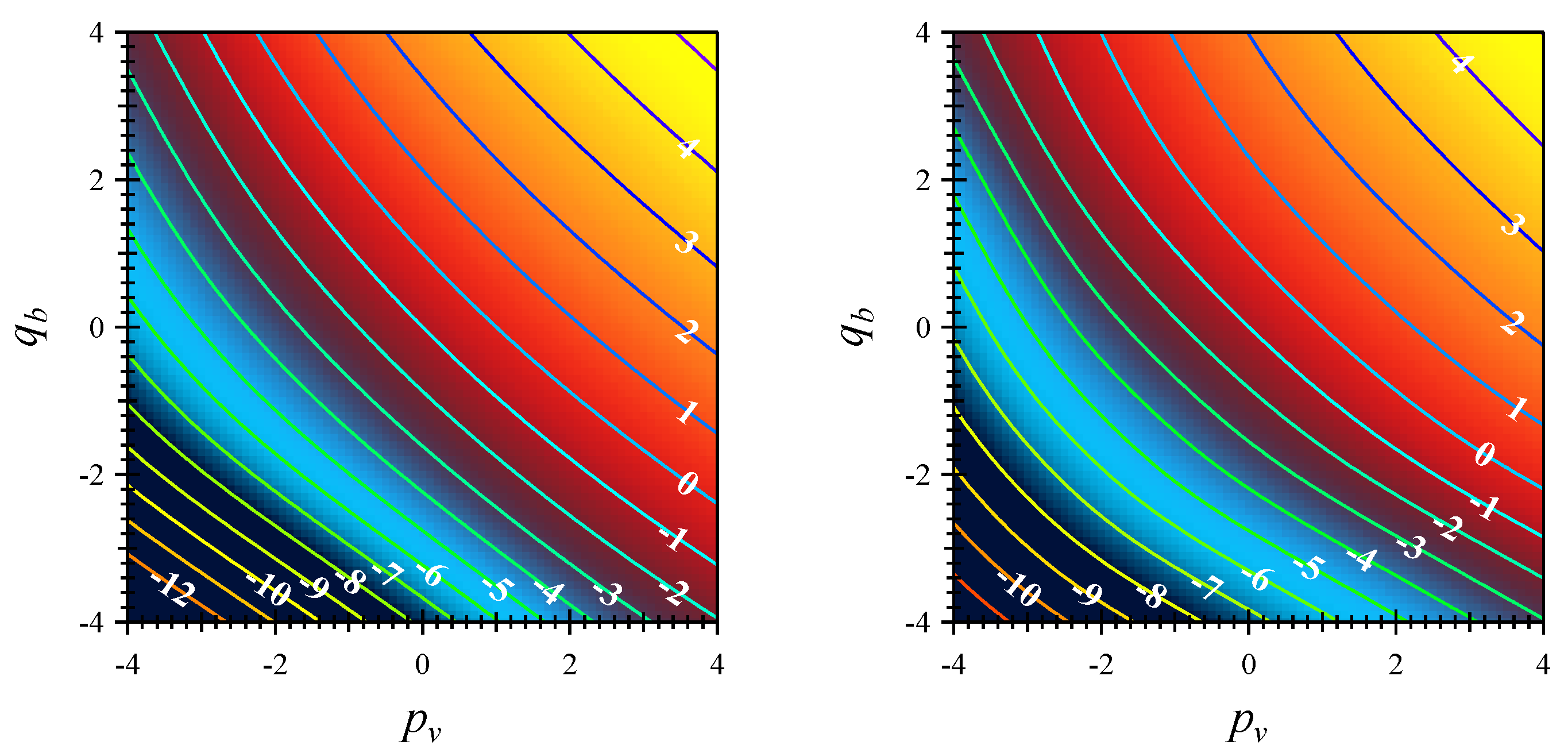
Using Equation (5), we computed the joint-scaling exponents, $\tau (q,p)$, as a function of the moments $(q,p)$. The results are depicted in Figure 7 for both intervals. Noticeable differences are observed among the joint-scaling exponents, $\tau (q,p)$, of the two periods. In particular, $\tau (q,p)$ for the fast solar wind covers a wide range of values.

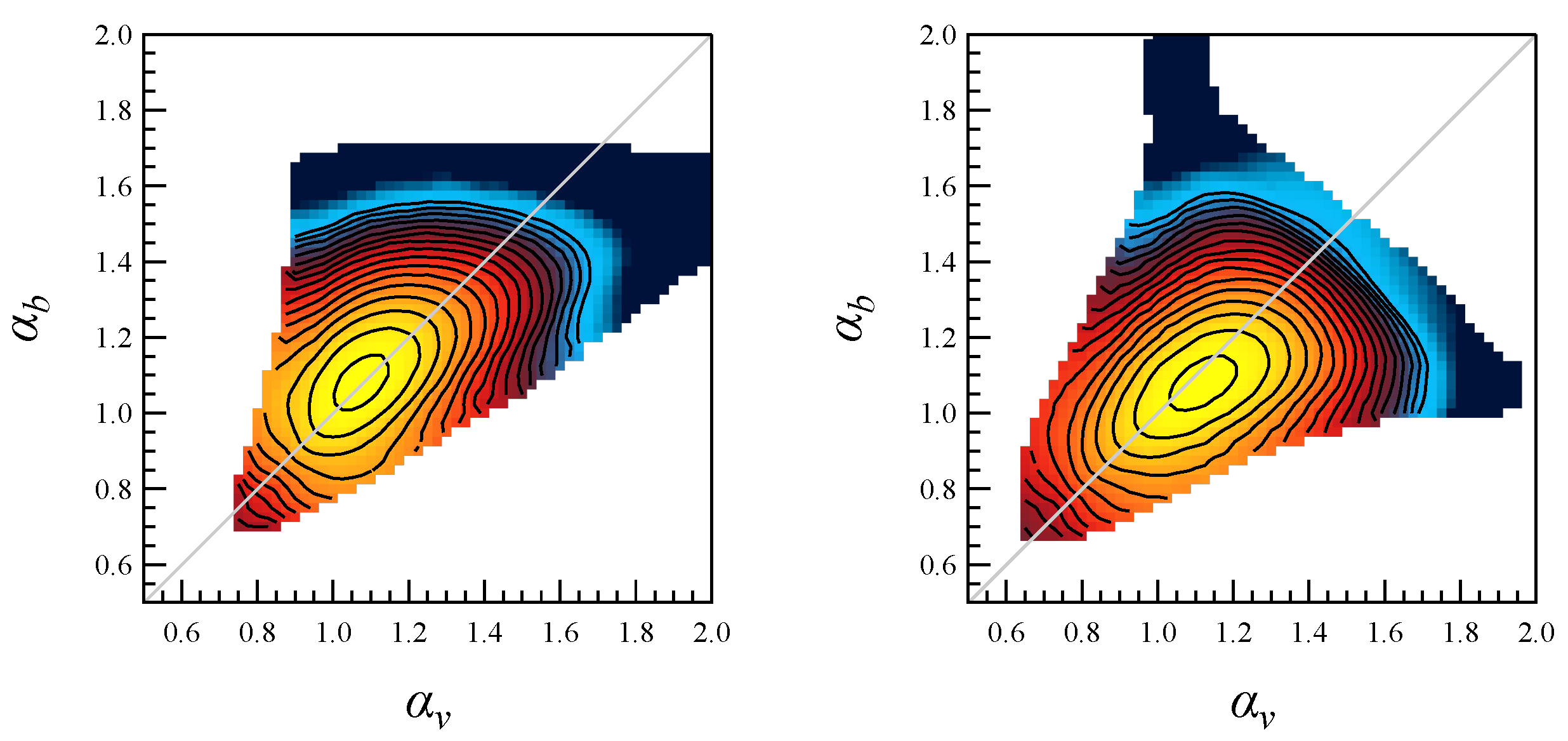
Using the double Legendre transforms in Equations (6)–(8), we evaluate the corresponding joint-singularity spectrum $f({\alpha }_v,{\alpha }_b)$. The results are presented in Figure 8.

The two joint-singularity spectra have distinct features. Both spectra are stretched along the bisector line, suggesting that the singularities of the two chosen quantities have some correlation. This correlation becomes clearer when the joint-singularity spectra obtained from the analysis are compared to those obtained from the case of independent distributions (see Figure 5). However, the observed correlation is more pronounced in the case of the fast solar wind, where the core of the joint-singularity spectrum (the yellow area in Figure 8) appears symmetric with respect to the bisector line. However, despite having a similar shape to the fast solar wind spectrum, the joint-singularity spectrum for the slow solar wind appears to be less symmetric with respect to the bisector line. We performed an additional test to confirm the existence of a significant correlation in the joint-singularity spectra. To change the positions of the singularities, we shuffled the time series of the two measures associated with the magnetic and velocity fields. Following that, we ran the joint multifractal analysis on the shuffled measures. Figure 9 presents the results of this test for the fast solar wind case. The most notable finding is that the joint-singularity spectrum $f({\alpha }_v,{\alpha }_b)$ becomes fully circular, losing its elongated character. This significant shape change suggests that magnetic and velocity field singularities occur in a manner that is clearly correlated. The slow solar wind case also yielded a similar result.

5. Discussion and Conclusions

The analysis of the joint multifractal features of the magnetic and velocity fields in turbulent solar wind reveals a significant degree of correlation between the multifractal characteristics of the two quantities. The correlation degree can be estimated by computing the corresponding correlation coefficient, which, according to Meneveau et al. [15], is defined as follows:

$$r=\frac{-{\partial }_{q,p}^2\tau }{\sqrt{{\partial }_q^2\tau {\partial }_p^2\tau }}{|}_{q=p=0}=\frac{-{\partial }_{p,q}^2\tau }{\sqrt{{\partial }_q^2\tau {\partial }_p^2\tau }}{|}_{q=p=0}.$$

(14)

In our case, the correlation coefficients for fast and slow solar wind are of $r=0.53$ and $r=0.60$. These correlation values are considered very high according to the conventional classification, where $r=0.5$ denotes a strong correlation.

Examining the two joint multifractal spectra in Figure 8 reveals that the slow solar wind has a broader range of singularities. Furthermore, the significant amplitude along the ${\alpha }_b$ direction suggests that the magnetic field is more intermittent than the velocity field. When the slow solar wind case is compared to the fast solar wind case, it is clear that the magnetic field in the slow solar wind is more intermittent. This observation is supported by the values of the individual intermittency exponents of the two measures [15], denoted as:

$$\begin{array}{c}\hfill {\mu }_b=-\frac{{\partial }^2}{\partial q^2}\tau (q,p){|}_{q=p=0},\end{array}$$

(15)

$$\begin{array}{c}\hfill {\mu }_v=-\frac{{\partial }^2}{\partial p^2}\tau (q,p){|}_{q=p=0}.\end{array}$$

(16)

These values are reported in

Table 2. Values of the individual intermittency exponents of the two measures (see Equations (15) and (16)).

Period	${\mathit{\mu }}_{\mathit{b}}$	${\mathit{\mu }}_{\mathit{v}}$
# 1: fast	$0.158$	$0.160$
# 2: slow	$0.235$	$0.143$

. While the fast solar wind shows nearly identical intermittent exponents for both individual measures, the slow solar wind exhibits different values, and notably, the intermittent exponent associated with the magnetic field is significantly larger than the others.

A possible explanation for the observed features could be the different degree of Alfvénicity between fast and slow solar wind. In the case of Alfvénic turbulence, a high degree of correlation is expected between magnetic and velocity field fluctuations [3]. To investigate this further, we can compute the normalized cross-helicity ${\sigma }_C$ and the normalized residual energy ${\sigma }_R$ as follows:

$$\begin{array}{c}\hfill {\sigma }_C=\frac{2\langle \mathbf{v}·\mathbf{b}\rangle }{\langle {\mathbf{v}}^2\rangle +\langle {\mathbf{b}}^2\rangle }\end{array}$$

(17)

$$\begin{array}{c}\hfill {\sigma }_R=\frac{\langle {\mathbf{v}}^2\rangle -\langle {\mathbf{b}}^2\rangle }{\langle {\mathbf{v}}^2\rangle +\langle {\mathbf{b}}^2\rangle }\end{array}$$

(18)

where $\langle \dots \rangle$ represents the time average over a certain interval T [22,23,24]. These two quantities provide information about the different roles of magnetic and kinetic energies and the relations between field fluctuations. Specifically, ${\sigma }_C$ measures the energy balance between outward- and inward-propagating Alfvénic fluctuations, while ${\sigma }_R$ quantifies the balance between kinetic and magnetic energy. Both quantities can vary within the range of [−1, +1].

Figure 10 displays the joint histogram of ${\sigma }_C$ and ${\sigma }_R$ computed at a 1 h scale. The distributions exhibit a significant difference. Specifically, the fast solar wind shows a more Alfvénic nature, whereas the slow solar wind appears to be characterized by non-Alfvénic fluctuations. This result supports the existence of magnetic field structures (see, e.g., Refs. [22,23]). Therefore, the more intermittent character of the magnetic field measure can be attributed to the presence of singularities associated with magnetic structures, such as flux tubes and shocks.

We presented an advancement in the analysis of the intermittency in solar wind in this study, as it investigates the correlation between the singularity character of magnetic field and velocity fluctuations in a novel way. The obtained results show a strong correlation between the singular character of the measure defined on the magnetic field and the one on the velocity field in the inertial range of solar wind. This implies that the source of this correlation must be found in the Alfvénic nature of solar wind turbulence. Furthermore, the study emphasizes the importance of magnetic structures such as flux tubes and shocks in shaping the correlation observed in the intermittent nature of the two quantities in the case of solar wind at 5 au [22,23,24]. What makes this research interesting is the use of the joint multifractal analysis method in the context of solar wind properties. By adopting this innovative approach, it is possible to gain a deeper understanding of how different solar wind quantities are interconnected, unveiling a multifaceted view of solar wind’s behavior.

In conclusion, this study offers valuable new insights into solar wind turbulence, shedding light on the complex dynamics of the heliosphere. By employing cutting-edge analysis methods, it sets the stage for further exploration of space plasma turbulence.