Numerical Solutions of the Multi-Space Fractional-Order Coupled Korteweg–De Vries Equation with Several Different Kernels

Abstract

In this article, the authors propose to investigate the numerical solutions of several fractional-order models of the multi-space coupled Korteweg–De Vries equation involving many different kernels. In order to transform these models into a set or system of differential equations, various properties of the first-kind Chebyshev polynomial are used in this study. The main objective of the present study is to apply the spectral collocation approach for the multi-space fractional-order coupled Korteweg–De Vries equation with different kernels. We use finite differences to numerically solve these differential equations by reducing them to algebraic equations. The Newton (or, more precisely, the Newton–Raphson) method is then used to solve these resulting algebraic equations. By calculating the error involved in our approach, the precision of the numerical solution is verified. The use of spectral methods, which provide excellent accuracy and exponential convergence for issues with smooth solutions, is shown to be a benefit of the current study.

1. Introduction

Fractional calculus is a branch of mathematics that generalizes the concepts of differentiation and integration to non-integer orders. Thus, instead of restricting differentiation and integration to whole numbers or integer orders, fractional calculus allows for differentiation and integration with non-integer or fractional orders (see, for details, [1,2,3,4,5,6,7]). The concept of fractional calculus dates back to the 17th century, with early contributions by mathematicians like Isaac Newton and Gottfried Leibniz. However, it was not until the 19th century that mathematicians such as Augustin-Louis Cauchy and Karl Weierstrass began to develop a systematic theory of fractional calculus. Fractional derivatives and integrals can be defined by using various approaches, such as the Riemann–Liouville, Liouville–Caputo (see [8]), or Grünwald–Letnikov definitions. These definitions involve extending the classical derivative and the classical integral operators to accommodate non-integer orders (see [9]). Fractional calculus has found applications in various fields, including physics, engineering, signal processing, and finance. It allows for a more nuanced understanding of the phenomena that exhibit fractional or fractal behavior, such as anomalous diffusion, viscoelasticity, and fractal time series (see [10,11,12,13,14,15]). Moreover, fractional calculus provides a powerful mathematical tool for the modeling and analysis of complex systems that cannot be adequately described by using the traditional integer-order calculus (see [16]).

In general, the Korteweg–De Vries (KdV) equations are found in the study of nonlinear dispersive waves (see [17]). These equations were introduced in 1895 by Korteweg and de Vries for modeling shallow water waves in a canal [18]. The coupled Korteweg–De Vries (cKdV) equation is a nonlinear partial differential equation that describes the evolution of two or more interacting, long, and weakly nonlinear waves in a dispersive medium. It is an extension of the well-known Korteweg–De Vries (KdV) equation, which describes the behavior of a single wave. Hirota and Satsuma in [19] introduced the coupled KdV equation. The KdV equations describe the interaction between two long waves that have different dispersion relations [19] (see also [20]). Interestingly, the Korteweg–De Vries equations appear in various fields of the physical sciences, such as plasmas, fluids, and crystal lattice vibrations at low temperatures. Despite the seemingly unrelated nature of these applications, they all originate from a general physical model and eventually converge to the Korteweg–De Vries equation when a specific limit of the problem is considered. Hence, the Korteweg–De Vries equation is considered to be universal in this context.

Lanre Akinyemi and Olaniyi S. Iyiola [21] used an effective method, the q-homotopy analysis transform method, to investigate a linked nonlinear Caputo fractional time system of equations. The generalized Hirota–Satsuma coupled with coupled KdV and the modified coupled KdV equations, which are used as a model in nonlinear physical phenomena arising in biology, chemistry, physics, and engineering, are the nonlinear fractional coupled systems studied in this current investigation. Basim Albuohimad et al. [22] offered a numerical approach capable of resolving a set of partial differential equations that are time-fractional. They employed the finite difference method for the time-fractional derivative and the spectrum collection method based on shifted Chebyshev polynomials in space. They also used this approach to solve the coupled time-fractional Korteweg–De Vries equations (KdV) under suitable initial and boundary conditions.

The use of Chebyshev polynomials in spectral methods is widely recognized for solving ordinary differential equations and partial differential equations (see [23,24,25]). When dealing with smooth problems in straightforward geometries, these methods demonstrate exponential convergence rates or spectral precision. A significant benefit of these methods compared to finite-difference approaches is that the computation of the approximation coefficient fully determines the solution at any desired point within the interval. As a result, the numerical solution of the system in Equation (1) below by utilizing operational matrix spectral methods based on the Chebyshev polynomials holds great significance (see also [26,27,28]).

The main objective in this paper is to present the numerical solutions of the multi-space fractional-order coupled Korteweg–De Vries equation by using several different kernels. The solution technique involves utilizing the shifted Chebyshev polynomials of the first kind and their properties along with the Chebyshev collocation method. This combination is employed to discretize the space fractional-order diffusion equation, resulting in a linear system of ordinary differential equations. This simplifies the problem significantly. The next step is to solve this system of ordinary differential equations by using the finite difference method (FDM) (see, for further details, [29,30,31]).

The structure of this paper is as follows. In Section 2, we review the first-kind Chebyshev polynomials and function approximation. In Section 3, we propose a spectral method based upon the shifted Chebyshev polynomials for solving the multi-space fractional-order coupled Korteweg–De Vries equation, which is associated with several different kernels. In Section 4, we provide numerical results and the discussion for the proposed system with the three kernels, which we have used in this paper. Finally, in Section 5, we present our conclusions.

2. The First-Kind Chebyshev Polynomials and Function Approximations

In this section, we will provide a quick review of the definitions and formulas related to the Chebyshev polynomials of the first kind.

It is well-known that the first-kind Chebyshev polynomials are defined on the interval $[-1,1]$ as follows (see, for details, [32,33]):

$$\begin{array}{c}\hfill T_n\left(\xi \right)=cos\left(n\theta \right)(n\in {\mathbb{N}}_0:=\mathbb{N}\cup \left\{0\right\}=0,1,2,\cdots ),\end{array}$$

(1)

where $\xi =cos\left(\theta \right).$

The Chebyshev polynomials ${\left\{T_n\left(\xi \right)\right\}}_{n\in {\mathbb{N}}_0}$ can be obtained from the following recurrence relation:

$$\begin{array}{c}\hfill T_{n+1}\left(\xi \right)=2\xi T_n\left(\xi \right)-T_{n-1}\left(\xi \right)(n\in \mathbb{N})\left(T_0\left(\xi \right)=1;T_1\left(\xi \right)=\xi \right).\end{array}$$

(2)

The Chebyshev polynomials ${\left\{T_n\left(\xi \right)\right\}}_{n\in {\mathbb{N}}_0}$ are orthogonal over the interval $[-1,1]$ with the weight function ${(1-{\xi }^2)}^{-\frac{1}{2}}$, and we have the following orthogonality property:

$$\begin{array}{cc}\hfill & {\int }_{-1}^1{(1-{\xi }^2)}^{-\frac{1}{2}}{T}_i\left(\xi \right)T_j\left(\xi \right)d\xi \hfill \\ \hfill & =\left\{\begin{array}{cc}0\hfill & (i\ne j)\hfill \\ \\ {\displaystyle \frac{\pi }{2}}\hfill & (i=j\ne 0)\hfill \\ \\ \pi \hfill & (i=j=0)\hfill \end{array}.\right.\hfill \end{array}$$

(3)

The explicit form of the Chebyshev polynomial is given as follows:

$$\begin{array}{c}\hfill T_n\left(\xi \right)=\frac{n}{2}\sum _{i=0}^{[n/2]}{(-1)}^i\frac{(n-i-1)!}{\left(i\right)!(n-2i)!}{\left(2\xi \right)}^{n-2i},\end{array}$$

(4)

where, as usual, $\left[\kappa \right]$ denotes the greatest integer in $\kappa \in \mathbb{R}$.

We define the shifted Chebyshev polynomials on the interval $[0,1]$ by setting the variable $\xi =2\zeta -1$. These polynomials are defined by

$${\overline{\mathbb{T}}}_s\left(\zeta \right)={\overline{\mathbb{T}}}_s(2\zeta -1)={\zeta }_{2s}\left(\sqrt{\zeta }\right),$$

where a family of orthogonal Chebyshev polynomials over the interval $[0,1]$ is formed by the polynomial set ${\left\{{\overline{\mathbb{T}}}_{2s}\left(\zeta \right)\right\}}_{s\in {\mathbb{N}}_0}$.

It is easy to compute the explicit form of the shifted Chebyshev polynomial ${\overline{\mathbb{T}}}_s\left(\zeta \right)$ of degree s as follows (see [33]):

$$\begin{array}{c}\hfill {\overline{\mathbb{T}}}_s\left(\zeta \right)=s\sum _{k=0}^s{(-1)}^{s-k}\frac{2^{2k}(s+k-1)!}{\left(2k\right)!(s-k)!}{\zeta }^k,\end{array}$$

(5)

where

$${\overline{\mathbb{T}}}_0\left(\zeta \right)=1\mathrm{and}{\overline{\mathbb{T}}}_1\left(\zeta \right)=2\zeta -1.$$

Upon expanding and approximating the function $\Omega \left(\zeta \right)$ over the range $[0,1]$ as a linear combination of the first $(m+1)$-terms of ${\overline{\mathbb{T}}}_s$, we find that

$$\Omega \left(\zeta \right)\simeq {\Omega }_m\left(\zeta \right)=\sum _{i=0}^m{a}_i{\overline{\mathbb{T}}}_i\left(\zeta \right),$$

(6)

where the coefficients $a_i$ are given by

$$\begin{array}{c}\hfill a_i=\left\{\begin{array}{cc}{\displaystyle \frac{1}{\pi }}{\int }_0^1{\displaystyle \frac{\Omega \left(\zeta \right){\overline{\mathbb{T}}}_i\left(\zeta \right)}{\sqrt{\zeta -{\zeta }^2}}}d\zeta \hfill & (i=0)\hfill \\ \\ {\displaystyle \frac{2}{\pi }}{\int }_0^1\frac{\Omega \left(\zeta \right){\overline{\mathbb{T}}}_i\left(\zeta \right)}{\sqrt{\zeta -{\zeta }^2}}d\zeta \hfill & (i\in \mathbb{N}).\hfill \end{array}\right.\end{array}$$

(7)

3. Implementation the Proposed Method and Numerical Simulation

We divide this section into three subsections, wherein describe the fractional derivatives associated with three different kernels.

3.1. Fractional Derivative Involving the Power-Law Kernel

We use a Sobolev space defined by

$$\begin{array}{c}\hfill H^1(0,b)=\left\{\phi \in L^2(0,b):\frac{d\phi }{d\zeta }\in L^2(0,b),L^2(0,b)=\{\phi \left(\zeta \right):{\left({\int }_0^b\phi {\left(\zeta \right)}^2\right)}^{\frac{1}{2}}<\infty \},\right\}\end{array}$$

(8)

to define the fractional derivative as follows.

Upon replacing the classical derivative with the fractional derivative involving a power-law kernel, the coupled KdV system of equations is given by

$$\begin{array}{c}\hfill {\alpha }_{\eta }+c{}^{\mathrm{LC}}{D}_{\zeta }^{{\nu }_1}\alpha +\gamma \alpha {}^{\mathrm{LC}}{D}_{\zeta }^{{\nu }_2}\alpha +\mu \beta {}^{\mathrm{LC}}{D}_{\zeta }^{{\nu }_2}\beta =0,\end{array}$$

(9)

and

$$\begin{array}{c}\hfill {\beta }_{\eta }+c{}^{\mathrm{LC}}{D}_{\zeta }^{{\nu }_1}\beta +\delta \alpha {}^{\mathrm{LC}}{D}_{\zeta }^{{\nu }_2}\beta =0,\end{array}$$

(10)

$$\left(2<{\nu }_1\le 3,0<{\nu }_2\le 1\right),$$

where ${}^{\mathrm{LC}}{D}_{\zeta }^{\nu }$ is the Liouville–Caputo (LC) fractional derivative of order $n-1<\nu \leqq n,n\in N$ of a function $\phi \left(\zeta \right)\in H^1(0,b)$ defined in the following form (see, for details, [34]):

$$\begin{array}{c}\hfill {}^{\mathrm{LC}}{D}_{\zeta }^{\nu }\phi \left(\zeta \right)=\frac{1}{\Gamma (n-\nu )}{\int }_0^{\zeta }\frac{{\phi }^{\left(n\right)}\left(\tau \right)}{{(\zeta -\tau )}^{\nu -n+1}}d\tau (\zeta >0).\end{array}$$

(11)

The first term in (9) stands for the evolution term, while the second and fourth terms are the nonlinear terms. The dispersion is the third term. The second term in (10) is the cross-nonlinear term; the first term in (10) is evolution once more; and the third term in (10) is dispersion once more, while $c,\gamma ,\delta$, and $\mu$ are constant parameters. The approximate formula in the case of the fractional derivative ${}^{\mathrm{LC}}{D}_{\zeta }^{\nu }\phi \left(\zeta \right)$ with the power-law kernel is given in the following theorem.

Theorem 1

(see [35]). Suppose that the function $\Omega \left(\zeta \right)$ is approximated in the form (6). Then, ${}^{\mathrm{LC}}{D}_{\zeta }^{\nu }\left({\Omega }_m\left(\zeta \right)\right)$ is given by

$$\begin{array}{c}\hfill {}^{\mathrm{LC}}{D}_{\zeta }^{\nu }\left({\Omega }_m\left(\zeta \right)\right)=\sum _{k=\lceil \nu \rceil }^m\sum _{\ell =\lceil \nu \rceil }^k{a}_i{\vartheta }_{k,\ell }{\Pi }_{\nu ,\ell }{}^{\mathrm{LC}},\end{array}$$

(12)

where

$$\begin{array}{c}\hfill {\vartheta }_{k,\ell }={(-1)}^{k-\ell }{2}^{2\ell }\frac{k(k+\ell -1)!}{\ell !(2k-2\ell )},\end{array}$$

(13)

and

$$\begin{array}{c}\hfill {\Pi }_{\nu ,\ell }{}^{\mathrm{LC}}\left(\zeta \right)=\frac{\Gamma (\ell +1)}{\Gamma (\ell -\nu +1)!};{\zeta }^{\ell -\nu }.\end{array}$$

(14)

We can now solve Equations (9) to (10) by using the Chebyshev spectral collocation method as follows:

$$\begin{array}{c}\hfill {\alpha }_m(\zeta ,\eta )=\sum _{k=0}^m{\alpha }_k\left(\eta \right){\overline{\mathbb{T}}}_k\left(\zeta \right),\end{array}$$

(15)

and

$$\begin{array}{c}\hfill {\beta }_m(\zeta ,\eta )=\sum _{k=0}^m{\beta }_k\left(\eta \right){\overline{\mathbb{T}}}_k\left(\zeta \right).\end{array}$$

(16)

By using Equations (9) to (10), (12), and Formula (6), we obtain

$$\begin{array}{cc}\hfill \sum _{k=0}^m\frac{d{\alpha }_k\left(\eta \right)}{d\eta }{\overline{\mathbb{T}}}_k\left(\zeta \right)& =c\sum _{k=\lceil {\nu }_1\rceil }^m\sum _{\ell =\lceil {\nu }_1\rceil }^k{\alpha }_k\left(\eta \right){\vartheta }_{k,\ell }{\Pi }_{\nu ,\ell }{}^{\mathrm{LC}}\left(\zeta \right)+\gamma \left(\sum _{k=0}^m{\alpha }_k\left(\eta \right){\overline{\mathbb{T}}}_k\left(\zeta \right)\right)\hfill \\ \hfill & ·\left(\sum _{k=\lceil {\nu }_2\rceil }^m\sum _{\ell =\lceil {\nu }_2\rceil }^k{\alpha }_k\left(\eta \right){\vartheta }_{k,\ell }{\Pi }_{\theta ,\ell }{}^{\mathrm{LC}}\left(\zeta \right)\right)+\mu \left(\sum _{k=0}^m{\beta }_k\left(\eta \right){\overline{\mathbb{T}}}_k\left(\zeta \right)\right)\hfill \\ \hfill & ·\left(\sum _{k=\lceil {\nu }_2\rceil }^m\sum _{\ell =\lceil {\nu }_2\rceil }^k{\beta }_k\left(\eta \right){\vartheta }_{k,\ell }{\Pi }_{\theta ,\ell }{}^{\mathrm{LC}}\left(\zeta \right)\right),\hfill \end{array}$$

(17)

and

$$\begin{array}{cc}\hfill \sum _{k=0}^m\frac{d{\beta }_k\left(\eta \right)}{d\eta }{\overline{\mathbb{T}}}_k\left(\zeta \right)& =c\sum _{k=\lceil {\nu }_1\rceil }^m\sum _{\ell =\lceil {\nu }_1\rceil }^k{\beta }_k\left(\eta \right){\vartheta }_{k,\ell }{\Pi }_{{\nu }_2,\ell }{}^{\mathrm{LC}}\left(\zeta \right)+\delta \left(\sum _{k=0}^m{\alpha }_k\left(\eta \right){\overline{\mathbb{T}}}_k\left(\zeta \right)\right)\hfill \\ \hfill & ·\left(\sum _{k=\lceil {\nu }_2\rceil }^m\sum _{\ell =\lceil {\nu }_2\rceil }^k{\beta }_k\left(\eta \right){\vartheta }_{k,\ell }{\Pi }_{\theta ,\ell }{}^{\mathrm{LC}}\left(\zeta \right)\right).\hfill \end{array}$$

(18)

Equations (17) and (18) will be collocated at m nodes ${\zeta }_p(p=0,1,\cdots ,m-1)$ as follows:

$$\begin{array}{cc}\hfill \sum _{k=0}^m\frac{d{\alpha }_k\left(\eta \right)}{d\eta }{\overline{\mathbb{T}}}_k\left({\zeta }_p\right)& =c\sum _{k=\lceil {\nu }_1\rceil }^m\sum _{\ell =\lceil {\nu }_1\rceil }^k{\alpha }_k\left(\eta \right){\vartheta }_{k,\ell }{\Pi }_{\theta ,\ell }{}^{\mathrm{LC}}\left({\zeta }_p\right)+\gamma \left(\sum _{k=0}^m{\alpha }_k\left(\eta \right){\overline{\mathbb{T}}}_k\left({\zeta }_p\right)\right)\hfill \\ & ·\left(\sum _{k=\lceil {\nu }_2\rceil }^m\sum _{\ell =\lceil {\nu }_2\rceil }^k{\alpha }_k\left(\eta \right){\vartheta }_{k,\ell }{\Pi }_{\theta ,\ell }{}^{\mathrm{LC}}\left({\zeta }_p\right)\right)+\mu \left(\sum _{k=0}^m{\beta }_k\left(\eta \right){\overline{\mathbb{T}}}_k\left({\zeta }_p\right)\right)\hfill \\ & ·\left(\sum _{k=\lceil {\nu }_2\rceil }^m\sum _{\ell =\lceil {\nu }_2\rceil }^k{\beta }_k\left(\eta \right){\vartheta }_{k,\ell }{\Pi }_{\theta ,\ell }{}^{\mathrm{LC}}\left({\zeta }_p\right)\right),\hfill \end{array}$$

(19)

$$\begin{array}{cc}\hfill \sum _{k=0}^m\frac{d{\beta }_k\left(\eta \right)}{d\eta }{\overline{\mathbb{T}}}_k\left({\zeta }_p\right)& =c\sum _{k=\lceil {\nu }_1\rceil }^m\sum _{\ell =\lceil {\nu }_1\rceil }^k{\beta }_k\left(\eta \right){\vartheta }_{k,\ell }{\Pi }_{\nu ,\ell }{}^{\mathrm{LC}}{\left({\zeta }_p\right)}_p+\delta \left(\sum _{k=0}^m{\alpha }_k\left(\eta \right){\overline{\mathbb{T}}}_k\left({\zeta }_p\right)\right)\hfill \\ \hfill & ·\left(\sum _{k=\lceil {\nu }_2\rceil }^m\sum _{\ell =\lceil {\nu }_2\rceil }^k{\beta }_k\left(\eta \right){\vartheta }_{k,\ell }{\Pi }_{\theta ,\ell }{}^{\mathrm{LC}}\left({\zeta }_p\right)\right).\hfill \end{array}$$

(20)

Additionally, by substituting from Equation (6), the corresponding initial conditions can be expressed. This leads to the following four equations:

$$\begin{array}{c}\hfill \sum _{k=0}^m{(-1)}^k\alpha \left(\eta \right)=g_1\left(\eta \right),\sum _{k=0}^m{(-1)}^k\beta \left(\eta \right)=h_1\left(\eta \right),\end{array}$$

(21)

$$\begin{array}{c}\hfill \sum _{k=0}^{m}2{(-1)}^{k-1}{k}^2\alpha \left(\eta \right)=g_2\left(\eta \right),\sum _{k=0}^{m}2{(-1)}^{k-1}{k}^2\beta \left(\eta \right)=h_2\left(\eta \right),\end{array}$$

(22)

and

$$\begin{array}{c}\hfill \sum _{k=0}^{m}2k^2\alpha \left(\eta \right)=g_3\left(\eta \right)\mathrm{and}\sum _{k=0}^{m}2k^2\beta \left(\eta \right)=h_3\left(\eta \right).\end{array}$$

(23)

Finally, by applying the finite difference method, we obtain a system of nonlinear algebraic equations, which can be solved numerically by using one of such well-known methods as, for example, the Newton–Raphson method to obtain ${\alpha }_k$ and ${\beta }_k$ for $k=0,1,\cdots ,m.$

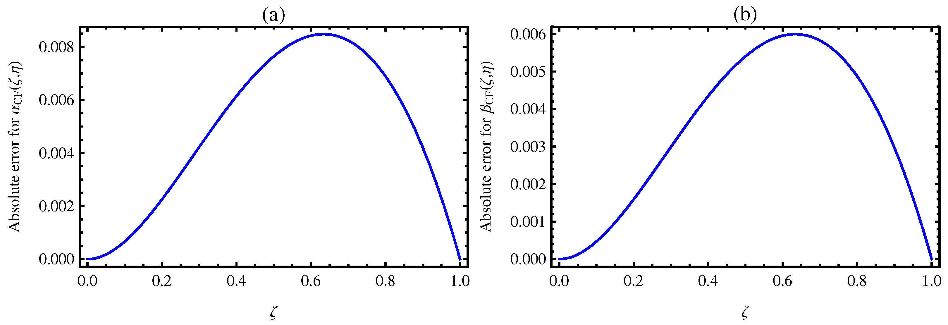
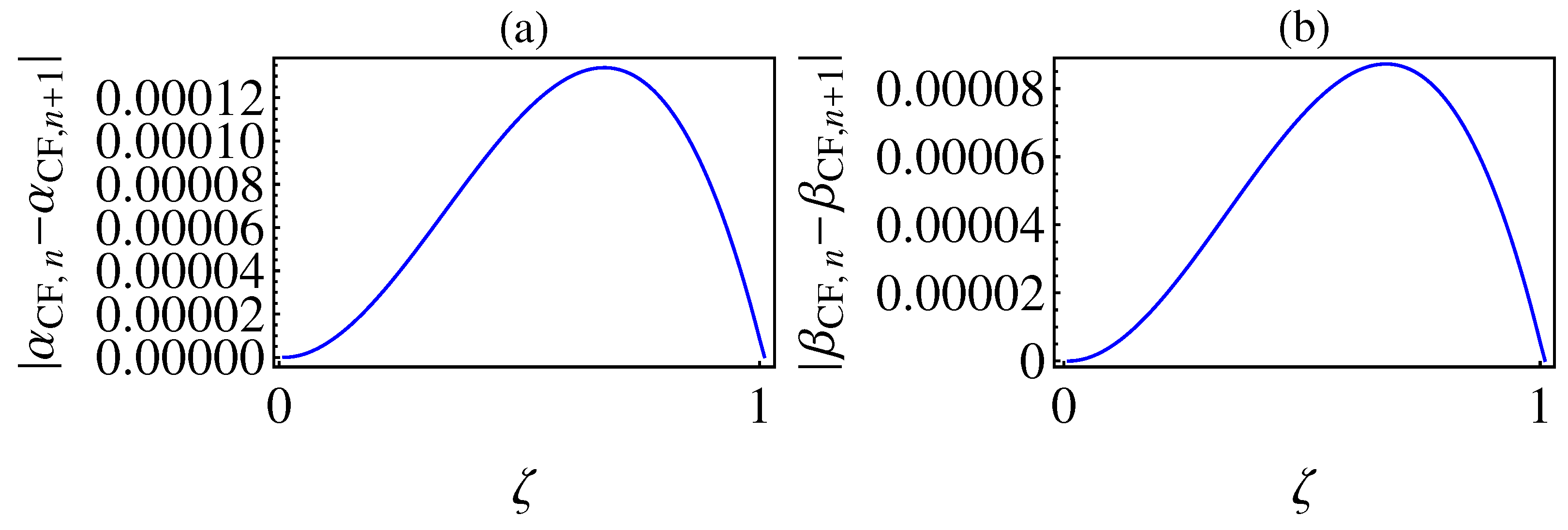
3.2. Fractional Derivative Involving the Exponential-Decay Kernel

After replacing the classical derivative by the fractional derivative with the exponential-decay kernel or by the Caputo–Fabrizio fractional-order derivative (CF), the coupled KdV system of equations can be written as follows:

$$\begin{array}{c}\hfill {\alpha }_{\eta }+c{}^{\mathrm{CF}}{D}_{\zeta }^{{\nu }_1}\alpha +\gamma \alpha {}^{\mathrm{CF}}{D}_{\zeta }^{{\nu }_2}\alpha +\mu \beta {}^{\mathrm{CF}}{D}_{\zeta }^{{\nu }_2}\beta =0,\end{array}$$

(24)

and

$$\begin{array}{c}\hfill {\beta }_{\eta }+c{}^{\mathrm{CF}}{D}_{\zeta }^{{\nu }_1}\beta +\delta \alpha {}^{\mathrm{CF}}{D}_{\zeta }^{{\nu }_2}\beta =0,\end{array}$$

(25)

$$\left(2<{\nu }_1\le 3,0<{\nu }_2\le 1\right),$$

where the fractional derivative ${}^{\mathrm{CF}}{D}_{\zeta }^{{\nu }_{.}}$ of order $0<\nu <1$ is defined in the following form (see [36]):

$$\begin{array}{c}\hfill {}^{\mathrm{CF}}{D}_{a+}^{\nu }\phi \left(\zeta \right)=\frac{\theta \left(\nu \right)}{1-\nu }{\int }_0^{\zeta }{e}^{-\frac{\nu (\zeta -\tau )}{1-\nu }}{\phi }^{{}^{\prime }}\left(\tau \right)d\tau ,\end{array}$$

(26)

where $\theta \left(\nu \right)$ is the normalization function.

The fractional derivative operator ${}^{\mathrm{CF}}{D}_{\zeta }^{\nu }$ of order $n<\nu <n+1$, involving the exponential-decay kernel, is defined as follows (see [37]):

$$\begin{array}{c}\hfill {}^{\mathrm{CF}}{D}_{a+}^{\nu }\phi \left(\zeta \right)={}^{\mathrm{CF}}{D}_{a+}^{\kappa }\left(D^n\phi \left(\zeta \right)\right)=\frac{\vartheta \left(\kappa \right)}{1-\kappa }{\int }_a^{\zeta }{\phi }^{(n+1)}\left(\tau \right)e^{-\frac{\kappa (\zeta -\tau )}{1-\kappa }}d\tau ,\end{array}$$

(27)

where $n=\lfloor \nu \rfloor$ = the floor function of $\nu$ (that is, the greatest integer less than or equal to $\nu$) and $\kappa =\lceil \nu \rceil$ = the ceiling function of $\nu$ (that is, the least integer greater than or equal to $\nu$).

Theorem 2

(see [37]). The left-sided fractional derivative involving the exponential-decay kernel of order $\nu \in (n,n+1)$ of the following function:

$$\phi \left(\zeta \right)={\zeta }^m(m>1;m\geqq \lceil \nu \rceil )$$

can be expressed in the following form:

$$\begin{array}{cc}\hfill & {}^{\mathrm{CF}}{D}_{0+}^{\nu }{\zeta }^m=\frac{M\left(\kappa \right)\Gamma (m+1)}{1-\kappa }\left(\sum _{i=0}^{m-n-1}\frac{{(-1)}^i{\zeta }^{m-n-1-i}}{\Gamma (m-n-i){\left(\frac{\kappa }{1-\kappa }\right)}^{i+1}}+\frac{{(-1)}^{m-n}}{{\left(\frac{\kappa }{1-\kappa }\right)}^{m-n}}{e}^{-\frac{\kappa \zeta }{1-\kappa }}\right).\hfill \end{array}$$

(28)

The formula in Theorem 1 of [37] at $a=0$ is a particular instance of Formula (28). See [37] for further information on the definitions and properties of fractional CF derivatives.

The following theorem presents the approximation formula of ${}^{\mathrm{CF}}{D}_{0+}^{\nu }{\Omega }_m\left(x\right)$ by means of (6).

Theorem 3.

The ${}^{\mathrm{CF}}{D}_{\zeta }^{\nu }\left({\Omega }_m\left(\zeta \right)\right)$ can be written as follows:

$$\begin{array}{c}\hfill {}^{\mathrm{CF}}{D}_{0+}^{\nu }\left({\Omega }_m\left(\zeta \right)\right)=\sum _{k=\lceil \nu \rceil }^m\sum _{\ell =\lceil \nu \rceil }^k{a}_k{\vartheta }_{k,\ell }{\Pi }_{k,\ell ,\kappa }{}^{\mathrm{CF}}\left(\zeta \right),\end{array}$$

(29)

where

$$\begin{array}{c}\hfill {\Pi }_{k,\ell ,\kappa }{}^{\mathrm{CF}}\left(\zeta \right)=\left(\frac{M\left(\kappa \right)}{1-\kappa }\right)\left(\frac{{(-1)}^{\ell -n}}{(\frac{\kappa }{1-\kappa }{)}^{\ell -n}}{e}^{-\frac{\kappa x}{1-\kappa }}+\sum _{p=0}^{\ell -n-1}\frac{{(-1)}^p{\zeta }^{\ell -n-1-p}}{\Gamma (\ell -n-p)(\frac{\kappa }{1-\kappa }{)}^{p+1}}\right).\end{array}$$

(30)

By using Equations (9) and (10), (12) and Formula (6) with CF, we obtain

$$\begin{array}{cc}\hfill \sum _{k=0}^m\frac{d{\alpha }_k\left(\eta \right)}{d\eta }{\overline{\mathbb{T}}}_k\left(\zeta \right)& =c\sum _{k=\lceil {\nu }_1\rceil }^m\sum _{\ell =\lceil {\nu }_1\rceil }^k{\alpha }_k\left(\eta \right){\vartheta }_{k,\ell }{\Pi }_{k,\ell ,\kappa }{}^{\mathrm{CF}}\left(\zeta \right)+\gamma \left(\sum _{k=0}^m{\alpha }_k\left(\eta \right){\overline{\mathbb{T}}}_k\left(\zeta \right)\right)\hfill \\ \hfill & ·\left(\sum _{k=\lceil {\nu }_2\rceil }^m\sum _{\ell =\lceil {\nu }_2\rceil }^k{\alpha }_k\left(\eta \right){\vartheta }_{k,\ell }{\Pi }_{k,\ell ,\kappa }{}^{\mathrm{CF}}\left(\zeta \right)\right)+\mu \left(\sum _{k=0}^m{\beta }_k\left(\eta \right){\overline{\mathbb{T}}}_k\left(\zeta \right)\right)\hfill \\ \hfill & ·\left(\sum _{k=\lceil {\nu }_2\rceil }^m\sum _{\ell =\lceil {\nu }_2\rceil }^k{\beta }_k\left(\eta \right){\vartheta }_{k,\ell }{\Pi }_{k,\ell ,\kappa }{}^{\mathrm{CF}}\left(\zeta \right)\right),\hfill \end{array}$$

(31)

$$\begin{array}{cc}\hfill \sum _{k=0}^m\frac{d{\beta }_k\left(\eta \right)}{d\eta }{\overline{\mathbb{T}}}_k\left(\zeta \right)& =c\sum _{k=\lceil {\nu }_1\rceil }^m\sum _{\ell =\lceil {\nu }_1\rceil }^k{\beta }_k\left(\eta \right),{\vartheta }_{k,\ell }{\Pi }_{k,\ell ,\kappa }{}^{\mathrm{CF}}\left(\zeta \right)+\delta \left(\sum _{k=0}^m{\alpha }_k\left(\eta \right){\overline{\mathbb{T}}}_k\left(\zeta \right)\right)\hfill \\ \hfill & ·\left(\sum _{k=\lceil {\nu }_2\rceil }^m\sum _{\ell =\lceil {\nu }_2\rceil }^k{\beta }_k\left(\eta \right){\vartheta }_{k,\ell }{\Pi }_{k,\ell ,\kappa }{}^{\mathrm{CF}}\left(\zeta \right)\right).\hfill \end{array}$$

(32)

Equations (31) and (32) will be collocated at m nodes ${\zeta }_p(p=0,1,\cdots ,m-1)$ as follows:

$$\begin{array}{cc}\hfill \sum _{k=0}^m\frac{d{\alpha }_k\left(\eta \right)}{d\eta }{\overline{\mathbb{T}}}_k\left({\zeta }_p\right)& =c\sum _{k=\lceil {\nu }_1\rceil }^m\sum _{\ell =\lceil {\nu }_1\rceil }^k{\alpha }_k\left(\eta \right),{\vartheta }_{k,\ell }{\Pi }_{k,\ell ,\kappa }{}^{\mathrm{CF}}\left({\zeta }_p\right)+\delta \left(\sum _{k=0}^m{\alpha }_k\left(\eta \right){\overline{\mathbb{T}}}_k\left(\zeta \right)\right)\hfill \\ \hfill & ·\left(\sum _{k=\lceil \nu \rceil }^m\sum _{\ell =\lceil \nu \rceil }^k{\alpha }_k\left(\eta \right){\vartheta }_{k,\ell }{\Pi }_{k,\ell ,\kappa }{}^{\mathrm{CF}}\left({\zeta }_p\right)\right)+\mu \left(\sum _{k=0}^m{\beta }_k\left(\eta \right){\overline{\mathbb{T}}}_k\left({\zeta }_p\right)\right)\hfill \\ \hfill & ·\left(\sum _{k=\lceil {\nu }_2\rceil }^m\sum _{\ell =\lceil {\nu }_2\rceil }^k{\beta }_k\left(\eta \right){\vartheta }_{k,\ell }{\Pi }_{k,\ell ,\kappa }{}^{\mathrm{CF}}\left({\zeta }_p\right)\right),\hfill \end{array}$$

(33)

and

$$\begin{array}{cc}\hfill \sum _{k=0}^m\frac{d{\beta }_k\left(\eta \right)}{d\eta }{\overline{\mathbb{T}}}_k\left(\zeta \right)& =c\sum _{k=\lceil {\nu }_1\rceil }^m\sum _{\ell =\lceil {\nu }_1\rceil }^k{\beta }_k\left(\eta \right){\vartheta }_{k,\ell }{\Pi }_{k,\ell ,\kappa }{}^{\mathrm{CF}}\left({\zeta }_p\right)+\delta \left(\sum _{k=0}^m{\alpha }_k\left(\eta \right){\overline{\mathbb{T}}}_k\left({\zeta }_p\right)\right)\hfill \\ \hfill & ·\left(\sum _{k=\lceil {\nu }_2\rceil }^m\sum _{\ell =\lceil {\nu }_2\rceil }^k{\beta }_k\left(\eta \right){\vartheta }_{k,\ell }{\Pi }_{k,\ell ,\kappa }{}^{\mathrm{CF}}\left({\zeta }_p\right)\right).\hfill \end{array}$$

(34)

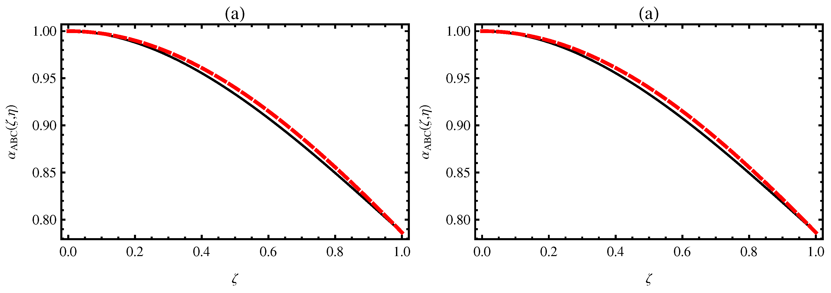
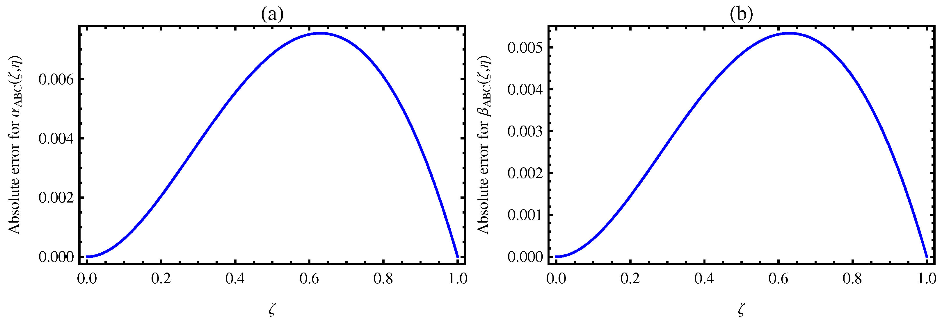
3.3. Fractional Derivative Involving the Mittag–Leffler Kernel

If we replace the classical derivative by the fractional derivative with the Mittag–Leffler kernel or the Atangana–Baleanu–Caputo fractional-order derivative (ABC), the coupled KdV system of the equations is given by

$$\begin{array}{c}\hfill {\alpha }_{\eta }+c{}^{\mathrm{ABC}}{D}_{\zeta }^{{\nu }_1}\alpha +\gamma \alpha {}^{\mathrm{ABC}}{D}_{\zeta }^{{\nu }_2}\alpha +\mu \beta {}^{\mathrm{ABC}}{D}_{\zeta }^{{\nu }_2}\beta =0,\end{array}$$

(35)

and

$$\begin{array}{c}\hfill {\beta }_{\eta }+c{}^{\mathrm{ABC}}{D}_{\zeta }^{{\nu }_1}\beta +\delta \alpha {}^{\mathrm{ABC}}{D}_{\zeta }^{{\nu }_2}\beta =0,\end{array}$$

(36)

$$\left(2<{\nu }_1\le 3,0<{\nu }_2\le 1\right),$$

where the fractional derivative ${{}_a^{\mathrm{ABC}}D}^{\nu }$ of order $0<\nu \leqq 1$ is defined in the following form (see [38]):

$$\begin{array}{c}\hfill {}_a^{\mathrm{ABC}}{D}^{\nu }\phi \left(\zeta \right)=\frac{M\left(\nu \right)}{1-\nu }{\int }_a^{\zeta }{\phi }^{\prime }\left(\tau \right)E_{\nu }\left(-\frac{\nu }{1-\nu }{(\zeta -\tau )}^{\nu }\right)d\tau ,\end{array}$$

(37)

where $M\left(\nu \right)=-\nu +\frac{\nu }{\Gamma \left(\nu \right)}+1$ is the normalization function such that $M\left(0\right)=M\left(1\right)=1$ and

$$E_{\nu }\left(\zeta \right)=\sum _{k=0}^{\infty }\frac{{\zeta }^k}{\Gamma (k\nu +1)}$$

is the Mittag–Leffler function (see, for details, (Section 1, [1]).

The fractional derivative ${{}_a^{\mathrm{ABC}}D}^{\nu }$ of order $n<\nu \leqq n+1$ is defined by (see [39])

$$\begin{array}{cc}\hfill {{}_a^{\mathrm{ABC}}D}^{\nu }\phi \left(\zeta \right)& ={{}_a^{\mathrm{ABC}}D}^{\kappa }\left(D^n\phi \left(\zeta \right)\right)\hfill \\ \hfill & =\frac{M\left(\kappa \right)}{1-\kappa }{\int }_a^{\zeta }{\phi }^{(n+1)}\left(\tau \right)E_{\kappa }\left(-\frac{\kappa }{1-\kappa }{(\zeta -\tau )}^{\kappa }\right)d\tau ,\hfill \end{array}$$

where $n=\lfloor \nu \rfloor$ = the floor function of $\nu$ (that is, the greatest integer less than or equal to $\nu$) and $\kappa =\lceil \nu \rceil$ = the ceiling function of $\nu$ (that is, the least integer greater than or equal to $\nu$).

Theorem 4

(see [31]). The ABC-derivative of order $\nu \in (n,n+1]$ of the following function:

$$\phi \left(\zeta \right)={\zeta }^m(m>1;\beta \geqq \lceil \nu \rceil )$$

is given by

$$\begin{array}{c}\hfill {{}_0^{\mathrm{ABC}}D}^{\nu }{\zeta }^m=\frac{M\left(\kappa \right)\Gamma (m+1)}{1-\kappa }\sum _{i=0}^{\infty }{\left(-\frac{\kappa }{1-\kappa }\right)}^i\frac{{\zeta }^{m+i\kappa -n}}{\Gamma (m+i\kappa -n+1)}.\end{array}$$

(38)

In the following theorem, we present the main approximation formula for ${}_0{}^{\mathrm{ABC}}{D}^{\nu }{\Omega }_m\left(\zeta \right)$ by applying the approximation (6).

Theorem 5

(see [31]). The ABC-derivative ${{}_0^{\mathrm{ABC}}D}^{\nu }\left({\Omega }_m\left(\zeta \right)\right)$ can be expressed as follows:

$${{}_0^{\mathrm{ABC}}D}^{\nu }\left({\Omega }_m\left(x\right)\right)=\sum _{i=\lceil \nu \rceil }^m\sum _{j=\lceil \nu \rceil }^i{a}_i{\vartheta }_{k,\ell }{\Pi }_{k,\ell ,\kappa }{}^{\mathrm{ABC}}\left(\zeta \right),$$

(39)

where

$$\begin{array}{cc}\hfill & {\Pi }_{k,\ell ,\kappa }{}^{\mathrm{ABC}}\left(\zeta \right)=\frac{M\left(\kappa \right)\Gamma (\ell +1)}{1-\kappa }\sum _{p=0}^{\ell -n-1}\frac{{\rho }^p{\zeta }^{\ell +p\kappa -n}}{\Gamma (\ell +p\kappa -n+1)}.\hfill \end{array}$$

(40)

It is easily observed that

$$\begin{array}{cc}\hfill \sum _{k=0}^m\frac{d{\alpha }_k\left(\eta \right)}{d\eta }{\overline{\mathbb{T}}}_k\left(\zeta \right)& =c\sum _{k=\lceil {\nu }_1\rceil }^m\sum _{\ell =\lceil {\nu }_1\rceil }^k{\alpha }_k\left(\eta \right){\vartheta }_{k,\ell }{\Pi }_{k,\ell ,\kappa }{}^{\mathrm{ABC}}\left(\zeta \right)+\gamma \left(\sum _{k=0}^m{\alpha }_k\left(\eta \right){\overline{\mathbb{T}}}_k\left(\zeta \right)\right)\hfill \\ & ·\left(\sum _{k=\lceil {\nu }_2\rceil }^m\sum _{\ell =\lceil {\nu }_2\rceil }^k{\alpha }_k\left(\eta \right){\vartheta }_{k,\ell }{\Pi }_{k,\ell ,\kappa }{}^{\mathrm{ABC}}\left(\zeta \right)\right)+\mu \left(\sum _{k=0}^m{\beta }_k\left(\eta \right){\overline{\mathbb{T}}}_k\left(\zeta \right)\right)\hfill \\ & ·\left(\sum _{k=\lceil {\nu }_2\rceil }^m\sum _{\ell =\lceil {\nu }_2\rceil }^k{\beta }_k\left(\eta \right){\vartheta }_{k,\ell }{\Pi }_{k,\ell ,\kappa }{}^{\mathrm{ABC}}\left(\zeta \right)\right),\hfill \end{array}$$

(41)

$$\begin{array}{cc}\hfill \sum _{k=0}^m\frac{d{\beta }_k\left(\eta \right)}{d\eta }{\overline{\mathbb{T}}}_k\left(\zeta \right)& =c\sum _{k=\lceil {\nu }_1\rceil }^m\sum _{\ell =\lceil {\nu }_1\rceil }^k{\beta }_k\left(\eta \right),{\vartheta }_{k,\ell }{\Pi }_{k,\ell ,\kappa }{}^{\mathrm{ABC}}\left(\zeta \right)+\delta \left(\sum _{k=0}^m{\alpha }_k\left(\eta \right){\overline{\mathbb{T}}}_k\left(\zeta \right)\right)\hfill \\ \hfill & ·\left(\sum _{k=\lceil {\nu }_2\rceil }^m\sum _{\ell =\lceil {\nu }_2\rceil }^k{\beta }_k\left(\eta \right){\vartheta }_{k,\ell }{\Pi }_{k,\ell ,\kappa }{}^{\mathrm{ABC}}\left(\zeta \right)\right).\hfill \end{array}$$

(42)

Equations (41) and (42) will be collocated at m nodes ${\zeta }_p(p=0,1,\cdots ,m-1)$ as follows:

$$\begin{array}{cc}\hfill \sum _{k=0}^m\frac{d{\alpha }_k\left(\eta \right)}{d\eta }{\overline{\mathbb{T}}}_k\left({\zeta }_p\right)& =c\sum _{k=\lceil {\nu }_1\rceil }^m\sum _{\ell =\lceil {\nu }_1\rceil }^k{\alpha }_k\left(\eta \right),{\vartheta }_{k,\ell }{\Pi }_{k,\ell ,\kappa }{}^{\mathrm{ABC}}\left({\zeta }_p\right)+\gamma \left(\sum _{k=0}^m{\alpha }_k\left(\eta \right){\overline{\mathbb{T}}}_k\left(\zeta \right)\right)\hfill \\ \hfill & ·\left(\sum _{k=\lceil {\nu }_2\rceil }^m\sum _{\ell =\lceil {\nu }_2\rceil }^k{\alpha }_k\left(\eta \right){\vartheta }_{k,\ell }{\Pi }_{k,\ell ,\kappa }{}^{\mathrm{ABC}}\left({\zeta }_p\right)\right)+\mu \left(\sum _{k=0}^m{\beta }_k\left(\eta \right){\overline{\mathbb{T}}}_k\left({\zeta }_p\right)\right)\hfill \\ \hfill & ·\left(\sum _{k=\lceil {\nu }_2\rceil }^m\sum _{\ell =\lceil {\nu }_2\rceil }^k{\beta }_k\left(\eta \right){\vartheta }_{k,\ell }{\Pi }_{k,\ell ,\kappa }{}^{\mathrm{ABC}}\left({\zeta }_p\right)\right),\hfill \end{array}$$

(43)

and

$$\begin{array}{cc}\hfill \sum _{k=0}^m\frac{d{\beta }_k\left(\eta \right)}{d\eta }{\overline{\mathbb{T}}}_k\left(\zeta \right)& =c\sum _{k=\lceil {\nu }_1\rceil }^m\sum _{\ell =\lceil {\nu }_1\rceil }^k{\beta }_k\left(\eta \right){\vartheta }_{k,\ell }{\Pi }_{k,\ell ,\kappa }{}^{\mathrm{ABC}}\left({\zeta }_p\right)+\delta \left(\sum _{k=0}^m{\alpha }_k\left(\eta \right){\overline{\mathbb{T}}}_k\left({\zeta }_p\right)\right)\hfill \\ \hfill & ·\left(\sum _{k=\lceil {\nu }_2\rceil }^m\sum _{\ell =\lceil {\nu }_2\rceil }^k{\beta }_k\left(\eta \right){\vartheta }_{k,\ell }{\Pi }_{k,\ell ,\kappa }{}^{\mathrm{ABC}}\left({\zeta }_p\right)\right).\hfill \end{array}$$

(44)

4. Numerical Results and Discussion

In this section, by using the three schemes as above, we numerically evaluate the multi-space fractional-order coupled Korteweg–De Vries equation with three different kernels. Figure 1, Figure 2, Figure 3, Figure 4, Figure 5, Figure 6, Figure 7, Figure 8 and Figure 9 serve to illustrate the numerical results. All of the numerical results presented in this section will be in accordance with the values $c=1,$ $\mu =-6,$ $\gamma =6,$ $\delta =3,$ $\lambda =1$, and $a=1.$

In Figure 1, we compare the exact solution with the approximate solution of (9) and (10) in the case of the LC-derivative with (as indicated above) ${\nu }_1=2.9,$ ${\nu }_2=0.9,$ $c=1,$ $\mu =-6,$ $\gamma =6,$ $\delta =3$ $\lambda =1,$ and $a=1.$ The exact solution of the coupled Korteweg–De Vries equation in the case of classical case is given by

$$\begin{array}{c}\hfill \alpha (\zeta ,\eta )=\frac{\lambda }{a}{\mathrm{sech}}^2\left(\sqrt{\frac{\lambda }{4a}}(\zeta -\lambda \eta )\right),\end{array}$$

(45)

and

$$\begin{array}{c}\hfill \beta (\zeta ,\eta )=\frac{\lambda }{\sqrt{2a}}{\mathrm{sech}}^2\left(\sqrt{\frac{\lambda }{4a}}(\zeta -\lambda \eta )\right).\end{array}$$

(46)

We use the initial condition in the exact solution for the coupled Korteweg–De Vries equation by setting the time equal to zero. Then, the the initial values are given by

$$\begin{array}{c}\hfill \alpha \left(\zeta \right)=\frac{\lambda }{a}{\mathrm{sech}}^2\left(\sqrt{\frac{\lambda }{4a}}\zeta \right),\end{array}$$

(47)

and

$$\begin{array}{c}\hfill \beta \left(\zeta \right)=\frac{\lambda }{\sqrt{2a}}{\mathrm{sech}}^2\left(\sqrt{\frac{\lambda }{4a}}\zeta \right).\end{array}$$

(48)

Furthermore, the boundary conditions after setting $\eta =0$ are given by

$$\begin{array}{c}\hfill \alpha \left(\zeta \right)=\frac{\lambda }{a}{\mathrm{sech}}^2\left(\sqrt{\frac{\lambda }{4a}}(-\lambda \eta )\right),\end{array}$$

(49)

$$\begin{array}{c}\hfill \beta \left(\zeta \right)=\frac{\lambda }{\sqrt{2a}}{\mathrm{sech}}^2\left(\sqrt{\frac{\lambda }{4a}}(-\lambda \eta )\right),\end{array}$$

(50)

$$\begin{array}{c}\hfill {\alpha }_{\zeta }=-\frac{\lambda }{a}\sqrt{\frac{\lambda }{a}}tanh\left(\sqrt{\frac{\lambda }{4a}}\left(\lambda (-\eta )\right)\right){\mathrm{sech}}^2\left(\sqrt{\frac{\lambda }{4a}}\left(\lambda \eta \right)\right),\end{array}$$

(51)

and

$$\begin{array}{c}\hfill {\beta }_{\zeta }=-\frac{\lambda }{a}\sqrt{\frac{\lambda }{a}}tanh\left(\sqrt{\frac{\lambda }{4a}}\left(\lambda (-\eta )\right)\right){\mathrm{sech}}^2\left(\sqrt{\frac{\lambda }{4a}}\left(\lambda \eta \right)\right).\end{array}$$

(52)

We will use the above initial and boundary conditions in all of the computations in this work.

In Figure 2, we show the absolute error between the exact solutions (45) and (46) and the numerical solution (9) and (10) for the same parameters as in Figure 1.

Since the fractional-order equation does not have an exact solution, in this case, we will resort to studying the absolute value of the error between two successive steps.

In Figure 3, an illustration of the error between two successive steps is plotted. More precisely, all of the data in Figure 1, Figure 2 and Figure 3 are presented in

Table 1. The absolute error for (9) and (10) with ${\nu }_1=2.9,{\nu }_2=0.9,c=1,\mu =-6,\gamma =6,\delta =3,\lambda =1,$ and $a=1.$

$\mathit{\zeta }$	$|\mathit{\alpha }(\mathit{\zeta },\mathit{\eta })-{\mathit{\alpha }}_{\mathbf{LC}}({\mathit{\zeta }}_{\mathit{n}},{\mathit{\eta }}_{\mathit{n}})|$	$|\mathit{\beta }(\mathit{\zeta },\mathit{\eta })-{\mathit{\beta }}_{\mathbf{LC}}({\mathit{\zeta }}_{\mathit{n}},{\mathit{\eta }}_{\mathit{n}})|$	$|{\mathit{\alpha }}_{\mathbf{LC},\mathit{n}}-{\mathit{\alpha }}_{\mathbf{LC},\mathit{n}+1}|$	$|{\mathit{\beta }}_{\mathbf{LC},\mathit{n}}-{\mathit{\beta }}_{\mathbf{LC},\mathit{n}+1}|$
0.1	$6.22302\times {10}^{-4}$	$4.40034\times {10}^{-4}$	$7.37892\times {10}^{-6}$	$5.21768\times {10}^{-6}$
0.2	$2.10212\times {10}^{-3}$	$1.48643\times {10}^{-3}$	$2.63144\times {10}^{-5}$	$1.86071\times {10}^{-5}$
0.3	$3.93123\times {10}^{-3}$	$2.7798\times {10}^{-3}$	$5.18548\times {10}^{-5}$	$3.66669\times {10}^{-5}$
0.4	$5.69248\times {10}^{-3}$	$4.02519\times {10}^{-3}$	$7.90486\times {10}^{-5}$	$5.58958\times {10}^{-5}$
0.5	$7.05016\times {10}^{-3}$	$4.98522\times {10}^{-3}$	$1.02944\times {10}^{-4}$	$7.27923\times {10}^{-5}$
0.6	$7.73733\times {10}^{-3}$	$5.47112\times {10}^{-3}$	$1.18589\times {10}^{-4}$	$8.38552\times {10}^{-5}$
0.7	$7.5411\times {10}^{-3}$	$5.33236\times {10}^{-3}$	$1.21033\times {10}^{-4}$	$8.55831\times {10}^{-5}$
0.8	$6.2868\times {10}^{-3}$	$4.44544\times {10}^{-3}$	$1.05323\times {10}^{-4}$	$7.44746\times {10}^{-5}$
0.9	$3.82179\times {10}^{-3}$	$2.70242\times {10}^{-3}$	$6.65082\times {10}^{-5}$	$4.70284\times {10}^{-5}$
1	0	0	$3.63417\times {10}^{-7}$	$2.56975\times {10}^{-7}$

.

From the previous three figures, we find that the numerical solutions that we presented are accurate and have a very small error order. Especially when calculating the error between two successive steps, which is the goal of our work, we study the fractional-order equations. The data which support these figures is presented in Table 1, which shows the exact amount of error. These calculations and representation of the data were performed in the case of the LC-derivative.

In Figure 4, Figure 5 and Figure 6, the same study was carried out as in the case of LC, but in the presence of the CF-derivative operator. Also, in

Table 2. The absolute error for (24) and (25) with ${\nu }_1=2.9,{\nu }_2=0.9,c=1,\mu =-6,\gamma =6,\delta =3,\lambda =1,$ and $a=1.$

$\mathit{\zeta }$	$|\mathit{\alpha }(\mathit{\zeta },\mathit{\eta })-{\mathit{\alpha }}_{\mathbf{CF}}({\mathit{\zeta }}_{\mathit{n}},{\mathit{\eta }}_{\mathit{n}})|$	$|\mathit{\beta }(\mathit{\zeta },\mathit{\eta })-{\mathit{\beta }}_{\mathbf{CF}}({\mathit{\zeta }}_{\mathit{n}},{\mathit{\eta }}_{\mathit{n}})|$	$|{\mathit{\alpha }}_{\mathbf{CF},\mathit{n}}-{\mathit{\alpha }}_{\mathbf{CF},\mathit{n}+1}|$	$|{\mathit{\beta }}_{\mathbf{CF},\mathit{n}}-{\mathit{\beta }}_{\mathbf{CF},\mathit{n}+1}|$
$0.1$	$6.65154\times {10}^{-4}$	$4.70335\times {10}^{-4}$	$8.1039\times {10}^{-6}$	$5.27768\times {10}^{-6}$
0.2	$2.25449\times {10}^{-3}$	$1.59416\times {10}^{-3}$	$2.88921\times {10}^{-5}$	$1.88204\times {10}^{-5}$
0.3	$4.23119\times {10}^{-3}$	$2.99191\times {10}^{-3}$	$5.69297\times {10}^{-5}$	$3.70869\times {10}^{-5}$
0.4	$6.14957\times {10}^{-3}$	$4.34841\times {10}^{-3}$	$8.67817\times {10}^{-5}$	$5.65358\times {10}^{-5}$
0.5	$7.64533\times {10}^{-3}$	$5.40607\times {10}^{-3}$	$1.13013\times {10}^{-4}$	$7.36257\times {10}^{-5}$
0.6	$8.42296\times {10}^{-3}$	$5.95594\times {10}^{-3}$	$1.30189\times {10}^{-4}$	$8.48153\times {10}^{-5}$
0.7	$8.24102\times {10}^{-3}$	$5.82728\times {10}^{-3}$	$1.32874\times {10}^{-4}$	$8.65632\times {10}^{-5}$
0.8	$6.89625\times {10}^{-3}$	$4.87639\times {10}^{-3}$	$1.15634\times {10}^{-4}$	$7.5328\times {10}^{-5}$
0.9	$4.20746\times {10}^{-3}$	$2.97513\times {10}^{-3}$	$7.3033\times {10}^{-5}$	$4.75684\times {10}^{-5}$
1	$4.62223\times {10}^{-32}$	$3.23556\times {10}^{-32}$	$3.63417\times {10}^{-7}$	$2.56975\times {10}^{-7}$

, the data that are shown in Figure 4, Figure 5 and Figure 6 are clarified.

In Figure 7, Figure 8 and Figure 9, the numerical solutions of (41) and (42) are also studied in the presence of the ABC-derivative operator. Also, the corresponding

Table 3. The comparison of the exact solution with the approximate solution of (41) and (42) via the ABC-derivative with ${\nu }_1=2.9,{\nu }_2=0.9,c=1,\mu =-6,\gamma =6,\delta =3\lambda =1,$ and $a=1$

$\mathit{\zeta }$	$|\mathit{\alpha }(\mathit{\zeta },\mathit{\eta })-{\mathit{\alpha }}_{\mathbf{ABC}}({\mathit{\zeta }}_{\mathit{n}},{\mathit{\eta }}_{\mathit{n}})|$	$|\mathit{\beta }(\mathit{\zeta },\mathit{\eta })-{\mathit{\beta }}_{\mathbf{ABC}}({\mathit{\zeta }}_{\mathit{n}},{\mathit{\eta }}_{\mathit{n}})|$	$|{\mathit{\alpha }}_{\mathbf{ABC},\mathit{n}}-{\mathit{\alpha }}_{\mathbf{ABC},\mathit{n}+1}|$	$|{\mathit{\beta }}_{\mathbf{ABC},\mathit{n}}-{\mathit{\beta }}_{\mathbf{ABC},\mathit{n}+1}|$
$0.1$	$6.08166\times {10}^{-4}$	$4.30038\times {10}^{-4}$	$7.03329\times {10}^{-6}$	$4.97329\times {10}^{-6}$
0.2	$2.05186\times {10}^{-3}$	$1.45089\times {10}^{-3}$	$2.50855\times {10}^{-5}$	$1.77381\times {10}^{-5}$
0.3	$3.83228\times {10}^{-3}$	$2.70983\times {10}^{-3}$	$4.94355\times {10}^{-5}$	$3.49562\times {10}^{-5}$
0.4	$5.5417\times {10}^{-3}$	$3.91858\times {10}^{-3}$	$7.53619\times {10}^{-5}$	$5.32889\times {10}^{-5}$
0.5	$6.85384\times {10}^{-3}$	$4.84639\times {10}^{-3}$	$9.81436\times {10}^{-5}$	$6.9398\times {10}^{-5}$
0.6	$7.51116\times {10}^{-3}$	$5.31119\times {10}^{-3}$	$1.13059\times {10}^{-4}$	$7.9945\times {10}^{-5}$
0.7	$7.31022\times {10}^{-3}$	$5.16911\times {10}^{-3}$	$1.15388\times {10}^{-4}$	$8.15914\times {10}^{-5}$
0.8	$6.08576\times {10}^{-3}$	$4.30328\times {10}^{-3}$	$1.00407\times {10}^{-4}$	$7.09988\times {10}^{-5}$
0.9	$3.69457\times {10}^{-3}$	$2.61246\times {10}^{-3}$	$6.33975\times {10}^{-5}$	$4.48288\times {10}^{-5}$
1	$1.11022\times {10}^{-16}$	$1.11022\times {10}^{-16}$	$3.63417\times {10}^{-7}$	$2.56975\times {10}^{-7}$

shows the absolute error of the numerical solutions of (41) and (42). Through this study, we found that the resulting error amount in the numerical calculations is very small. Consequently, this work can be applied to other fractional-order systems and equations.

5. Conclusions

In our present investigation, the multi-space fractional-order coupled Korteweg–De Vries equation with several different kernels was effectively transformed first into a system of differential equations and then into a system of nonlinear algebraic equations. In order to solve the resulting system of nonlinear algebraic equations, we applied one of the widely-used numerical techniques, which is popularly known as the Newton–Raphson method. By computing the absolute error between the exact solutions and the approximate solutions, the accuracy of the considered approximations was confirmed. Also, in the case of the non-integer order, we computed the absolute error between the successive approximations.

In our future work, we propose to focus our attention on the use of fractional derivatives of space–time. Also, we will use nonstandard finite-difference methods to convert the fractional time derivative into a difference equation. In addition, we can employ other special functions to transform complicated models into a controllable system of differential equations (see, for example, [40]).

References

1. Kilbas, A.A.; Srivastava, H.M.; Trujillo, J.J. Theoryand Applications of Fractional Differential Equations; North-Holland Mathematical Studies; Elsevier (North-Holland) Science Publishers: Amsterdam, The Netherlands; London, UK; New York, NY, USA, 2006; Volume 204. [Google Scholar]
2. Podlubny, I. Fractional Differential Equations: An Introduction to Fractional Derivatives, Fractional Differential Equations, to Methods of Their Solution and Some of Their Applications; Mathematics in Science and Engineering; Academic Press: New York, NY, USA; London, UK; Sydney, Australia; Tokyo, Japan; Toronto, ON, Canada, 1999; Volume 198. [Google Scholar]
3. Hilfer, R. (Ed.) Applications of Fractional Calculus in Physics; World Scientific Publishing Company: Singapore; Hoboken, NJ, USA; London, UK; Hong Kong, China, 2000. [Google Scholar]
4. Shishkina, E.; Sitnik, S. Transmutations, Singular and Fractional Differential Equations with Applications to Mathematical Physics; Mathematics in Science and Engineering; Academic Press (Elsevier Science Publishers): New York, NY, USA; London, UK; Toronto, ON, Canada, 2020. [Google Scholar]
5. Anastassiou, G.A. Generalized Fractional Calculus: New Advancements and Applications; Studies in Systems, Decision and Control; Springer: Cham, Switzerland, 2021; Volume 305. [Google Scholar]
6. Mainardi, F. Fractional Calculus and Waves in Linear Viscoelasticity: An Introduction to Mathematical Models; World Scientific Publishing Company: Singapore; Hoboken, NJ, USA; London, UK; Hong Kong, China, 2010. [Google Scholar]
7. Samko, S.G.; Kilbas, A.A.; Marichev, O.I. Fractional Integrals and Derivatives: Theory and Applications; Gordon and Breach: Yverdon, Switzerland, 1993. [Google Scholar]
8. Liouville, J. Mémoire sur quelques quéstions de géometrie et de mécanique, et sur un nouveau genre de calcul pour résoudre ces quéstions. J. École Polytech. 1832, 13, 1–69. [Google Scholar]
9. Miller, K.S.; Ross, B. An Introduction to the Fractional Calculus and Fractional Differential Equations; John Wiley and Sons: New York, NY, USA; Chischester, UK; Brisbane, Australia; Toronto, ON, Canada,, 1993. [Google Scholar]
10. Sabir, Z.; Said, S.B.; Al-Mdallal, Q. A fractional order numerical study for the influenza disease mathematical model. Alex. Eng. J. 2023, 65, 615–626. [Google Scholar] [CrossRef]
11. Alqhtani, M.; Owolabi, K.M.; Saad, K.M. Spatiotemporal (target) patterns in sub-diffusive predator-prey system with the Caputo operator. Chaos Solitons Fractals 2022, 160, 112267. [Google Scholar] [CrossRef]
12. Abdon, M.A.; Hasan, F.L. Advantages of the differential equations for solving problems in mathematical physics with symbolic computation. Math. Model. Eng. Probl. 2022, 9, 268–276. [Google Scholar] [CrossRef]
13. Srivastava, H.M.; Saad, K.M.; Hamanah, W.M. Certain new models of the multi-space fractal-fractional Kuramoto-Sivashinsky and Korteweg-de Vries equations. Mathematics 2022, 10, 1089. [Google Scholar] [CrossRef]
14. Waheed, W.; Deng, G.; Liu, B. Discrete Laplacian operator and its Applications in signal processing. IEEE ACCESS 2020, 8, 89692–89707. [Google Scholar] [CrossRef]
15. Lin, Z.; Wang, H. Modeling and application of fractional-order economic growth model with time delay. Fractal Fract. 2021, 5, 74. [Google Scholar] [CrossRef]
16. Pakhira, R.; Ghosh, U.; Garg, H. An inventory model for partial backlogging items with memory effect. Soft Comput. 2023, 27, 9533–9550. [Google Scholar] [CrossRef]
17. Korteweg, D.J.; de Vries, G. On the change of form of long waves advancing in a rectangular canal, and on a new type of long stationary waves. Philos. Mag. 1985, 39, 422–443. [Google Scholar] [CrossRef]
18. Wu, Y.; Geng, X.; Hu, X.; Zhu, S. A generalized Hirota-Satsuma coupled Korteweg-de Vries equation and Miura transformations. Phys. Lett. A 1999, 255, 259–264. [Google Scholar] [CrossRef]
19. Hirota, R.; Satsuma, J. Soliton solutions of a coupled Korteweg-de Vries equation. Phys. Lett. A 1981, 85, 407–418. [Google Scholar] [CrossRef]
20. Srivastava, H.M.; Mandal, H.; Bira, B. Lie symmetry and exact solution of the time-fractional Hirota-Satsuma Korteweg-de Vries system. Russ. J. Math. Phys. 2021, 28, 284–292. [Google Scholar] [CrossRef]
21. Akinyemi, L.; Iyiola, O.S. A reliable technique to study nonlinear time-fractional coupled Korteweg-de Vries equations. Adv. Differ. Equ. 2020, 169, 2020. [Google Scholar] [CrossRef]
22. Albuohimad, B.; Adibi, H.; Kazem, S. A numerical solution of time-fractional coupled Korteweg-de Vries equation by using spectral collection method. Ain Shams Eng. J. 2018, 9, 1897–1905. [Google Scholar] [CrossRef]
23. Dabiri, A.; Butcher, E.A. Numerical solution of multi-order fractional differential equations with multiple delays via spectral collocation methods. Appl. Math. Model. 2018, 56, 424–448. [Google Scholar] [CrossRef]
24. Dabiri, A.; Butcher, E.A. Efficient modified Chebyshev differentiation matrices for fractional differential equations. Commun. Nonlinear Sci. Numer. Simul. 2017, 50, 284–310. [Google Scholar] [CrossRef]
25. Dabiri, A.; Butcher, E.A. Stable fractional Chebyshev differentiation matrix for the numerical solution of multi-order fractional differential equations. Nonlinear Dyn. 2017, 90, 185–201. [Google Scholar] [CrossRef]
26. Yang, X.-J.; Hristov, J.; Srivastava, H.M.; Ahmad, B. Modelling fractal waves on shallow water surfaces via local fractional Korteweg-de Vries equation. Abstr. Appl. Anal. 2014, 2014, 278672. [Google Scholar] [CrossRef]
27. Baleanu, D.; Shiri, B.; Srivastava, H.M.; Al Qurashi, M. A Chebyshev spectral method based on operational matrix for fractional differential equations involving non-singular Mittag-Leffler kernel. Adv. Differ. Equ. 2018, 2018, 353. [Google Scholar] [CrossRef]
28. Hadhoud, A.R.; Srivastava, H.M.; Rageh, A.A.M. Non-polynomial B-spline and shifted Jacobi spectral collocation techniques to solve time-fractional nonlinear coupled Burgers’ equations numerically. Adv. Differ. Equ. 2021, 2021, 439. [Google Scholar] [CrossRef]
29. Khader, M.M.; Saad, K.M. A numerical approach for solving the fractional Fisher equation using Chebyshev spectral collocation method. Chaos Solitons Fractals 2018, 110, 169–177. [Google Scholar] [CrossRef]
30. Khader, M.M.; Saad, K.M.; Hammouch, Z.; Baleanu, D. A spectral collocation method for solving fractional KdV and KdV-Burgers equations with non-singular kernel derivatives. Appl. Numer. Math. 2021, 161, 137–146. [Google Scholar] [CrossRef]
31. Khader, M.M.; Saad, K.M.; Gómez-Aguilar, J.F.; Baleanu, D. Numerical solutions of the fractional Fisher’s type equations with Atangana-Baleanu fractional derivative by using spectral collocation methods. Chaos 2019, 29, 023116. [Google Scholar]
32. Szegö, G. Orthogonal Polynomials, 4th ed.; American Mathematical Society Colloquium Publications; American Mathematical Society: Providence, RI, USA, 1975; Volume 23. [Google Scholar]
33. Mason, J.C.; Handscomb, D.C. Chebyshev Polynomials; Chapman and Hall (CRC Press): Baton Roca, FL, USA, 2003. [Google Scholar]
34. Srivastava, H.M. An introductory overview of fractional-calculus operators based upon the Fox-Wright and related higher transcendental functions. J. Adv. Eng. Comput. 2021, 5, 135–166. [Google Scholar] [CrossRef]
35. Sweilam N, H.; Khader, M.M. A Chebyshev pseudo-spectral method for solving fractional integro-differential equations. ANZIAM J. 2010, 51, 464–475. [Google Scholar] [CrossRef]
36. Caputo, M.; Fabrizio, M. A new definition of fractional derivative without singular kernel. Prog. Fract. Differ. Appl. 2015, 1, 1–13. [Google Scholar]
37. Loh, J.R.; Isah, A.; Phang, C.; Toh, Y.T. On the new properties of Caputo-Fabrizio operator and its application in deriving shifted Legendre operational matrix. Appl. Numer. Math. 2018, 132, 138–153. [Google Scholar] [CrossRef]
38. Atangana, A.; Baleanu, D. New fractional derivative with non-local and non-singular kernel. Therm. Sci. 2016, 20, 757–763. [Google Scholar] [CrossRef]
39. Abdeljawad, T.; Baleanu, D. Integration by parts and its applications of a new nonlocal fractional derivative with Mittag-Leffler nonsingular kernel. J. Nonlinear Sci. Appl. 2017, 9, 1098–1107. [Google Scholar] [CrossRef]
40. Srivastava, H.M. A survey of some recent developments on higher transcendental functions of analytic number theory and applied mathematics. Symmetry 2021, 13, 2294. [Google Scholar] [CrossRef]
Figure 1. Graph of the comparison of the exact solution with the approximate solution of (9) and (10) in (a) and (b) respectively in the case of the LC-derivative with ν 1 = 2.9 ,   ν 2 = 0.9 ,   c = 1 ,   μ = 6 ,   γ = 6 ,   δ = 3 ,   λ = 1 , and a = 1 (red dashed line: exact solution; black line: approximate solution).
Fractalfract 07 00716 g001
Figure 2. Graph of the absolute error of (9) and (10) in (a) and (b) respectively in the case of the LC-derivative with ν 1 = 2.9 , ν 2 = 0.9 , c = 1 ,   μ = 6 ,   γ = 6 ,   δ = 3 ,   λ = 1 , and a = 1 .
Fractalfract 07 00716 g002
Figure 3. Graph of the absolute error of the two steps of (9) and (10) in (a) and (b) respectively via LC with ν 1 = 2.9 , ν 2 = 0.9 , c = 1 ,   μ = 6 ,   γ = 6 ,   δ = 3 λ = 1 , and a = 1 .
Fractalfract 07 00716 g003
Figure 4. Graph of the comparison of the exact solution with the approximate solution of (24) and (25) in (a) and (b) respectively via the CF-derivative with ν 1 = 2.9 , ν 2 = 0.9 ,   c = 1 ,   μ = 6 ,   γ = 6 ,   δ = 3 ,   λ = 1 , and a = 1 (red dashed line: exact solution; black line: approximate solution).
Fractalfract 07 00716 g004
Figure 5. Graph of the absolute error of (24) and (25) in (a) and (b) respectively via the CF-derivative with ν 1 = 2.9 , ν 2 = 0.9 , c = 1 , μ = 6 ,   γ = 6 ,   δ = 3 ,   λ = 1 , and a = 1 .
Fractalfract 07 00716 g005
Figure 6. Graph of the absolute error of two step of (24) and (25) in (a) and (b) respectively via the CF-derivative with ν 1 = 2.9 , ν 2 = 0.9 , c = 1 ,   μ = 6 ,   γ = 6 ,   δ = 3 ,   λ = 1 and a = 1 .
Fractalfract 07 00716 g006
Figure 7. Graph of the comparison of the exact solution with the approximate solution of (41) and (42) in (a) and (b) respectively via the ABC-derivative with ν 1 = 2.9 , ν 2 = 0.9 ,   c = 1 ,   μ = 6 ,   γ = 6 ,   δ = 3 λ = 1 , and a = 1 (red dashed line: exact solution; black line: approximate solution).
Fractalfract 07 00716 g007
Figure 8. Graph of the absolute error of (41) and (42) in (a) and (b) respectively via the ABC-derivative with ν 1 = 2.9 , ν 2 = 0.9 , c = 1 ,   μ = 6 ,   γ = 6 ,   δ = 3 ,   λ = 1 , and a = 1 .
Fractalfract 07 00716 g008
Figure 9. Graph of the absolute error of the two steps of (41) and (42) in (a) and (b) respectively via the ABC-derivative with ν 1 = 2.9 , ν 2 = 0.9 ,   c = 1 ,   μ = 6 ,   γ = 6 ,   δ = 3 ,   λ = 1 and a = 1 .
Fractalfract 07 00716 g009