Article

The Dynamic Effects of COVID-19 and the March 2020 Crash on the Multifractality of NASDAQ Insurance Stock Markets

School of Finance, Shanghai University of Finance and Economics, Shanghai 200433, China
*
Author to whom correspondence should be addressed.
Fractal Fract. 2023, 7(1), 91; https://doi.org/10.3390/fractalfract7010091
Submission received: 29 October 2022 / Revised: 18 December 2022 / Accepted: 9 January 2023 / Published: 13 January 2023
(This article belongs to the Special Issue Fractal and Multifractal Analysis in Financial Markets)

Abstract

:
Triggered by COVID-19, one of the most dramatic crashes in the stock market in history occurred in March 2020. The sharp reductions in NASDAQ insurance stock indexes were observed after the occurrence of COVID-19 and in March 2020. In this study, the NASDAQ insurance stock markets (including NASDAQ Insurance Index, Developed Markets Insurance Index, and Emerging Markets Insurance Index) and NASDAQ Composite Index are utilized. The “scissors difference” between the NASDAQ Insurance Index and NASDAQ Composite Index is observed. The dynamic effects of the COVID-19 epidemic and the March 2020 crash on the multifractality of four series are explored. Firstly, the apparent and intrinsic multifractality, the components of multifractality, and the dynamic effects of the COVID-19 epidemic on these indexes are analyzed. Secondly, the multifractal cross-correlation between the NASDAQ Insurance Index and NASDAQ Composite Index is investigated. The dynamic influence of the COVID-19 epidemic on the cross-correlation is examined. The multifractal analysis results reveal that four series both before and after the occurrence of COVID-19 have multifractal characteristics. The stronger multifractal characteristics and the greater multifractal degree are obtained after the occurrence of COVID-19. The intrinsic multifractality of the three indexes ascends largely after the occurrence of COVID-19. The multifractal cross-correlation analysis illustrates that the cross-correlation between two indexes before and after the occurrence of COVID-19 is multifractal. The stronger multifractal cross-correlations and greater multifractal degrees are shown. The contribution of the intrinsic multifractal cross-correlation increased after the occurrence of COVID-19.

1. Introduction

Globally, there have been 620.88 million confirmed cases of COVID-19 and 6.54 million deaths as of 14 October 2022, according to the World Health Organization (the data were collected from WHO Coronavirus (COVID-19) Dashboard (https://covid19.who.int/, accessed on 16 October 2022)). The devastation brought by COVID-19 has caused severe damage not only to people’s health and life but also to the world economy. For 2020, the World Bank estimates a 4.3% contraction of the global economy, amounting to more than USD 3.7 trillion in lost output [1].
Triggered by COVID-19, one of the most dramatic crashes in the stock market in history occurred in March 2020. In barely seven trading days, the NASDAQ Composite Index plunged 20.1% and the NASDAQ Bank Index decreased 23.7% (March 4, 5, 6, 9, 10, 11, and 12, 2020). The NASDAQ Insurance Index dropped 25.4% (March 6, 9, 10, 11, 12, 13, and 16, 2020). Before and after the March 2020 crash, the NASDAQ Bank Index kept below the NASDAQ Composite Index. However, the “scissors difference” between the NASDAQ Insurance Index and the NASDAQ Composite Index is observed. This phenomenon drew our attention and began the study.
Numerous researchers have examined how COVID-19 affects the financial markets. Lan et al. investigated the shifts in systemic risks in China’s financial sector—which includes the banking, insurance, and securities sectors—during the COVID-19 epidemic. They discovered that systemic risks in the financial sector significantly increased following the COVID-19 epidemic [2]. Foglia et al. analyzed the extreme risk spillovers among 183 financial institutions in the Euro Area, which included banks, insurance firms, diversified financial firms, and real estate firms. They found that the risk spillover effect gets bigger when the market is exposed to a crisis [3].
It is usually argued that insurance firms are less risky than banks due to their lower liquidity risk exposure [4]. However, the operations of financial intermediaries have become more complex and possibly riskier as a result of the increasing interactions between the insurance sector and financial markets, and the rapid pace of financial innovation, globalization, and deregulation of the financial system [5]. Baluch et al. reported that during the 2007–2008 crisis, life insurance companies, global composite insurance companies, global reinsurance companies, and other European insurance companies were impacted the most and performed the worst [6]. Drake et al. showed that the financial crisis that occurred between 2007 and 2008 caused financial guarantee insurance companies to become financially strained, which had a negative impact on markets and businesses that depended on this insurance [7]. Babuna et al. illustrated the impact of COVID-19 on the insurance industry in Ghana, reporting that the financial results of insurance companies are poorer [8]. Farooq et al. analyzed the effects of COVID-19 on the stock returns of 958 insurance companies [9]. However, based on our knowledge, there is no empirical research on the effect of the COVID-19 epidemic and the March 2020 crash on the multifractality of the insurance stock markets. Accordingly, the purpose of this paper is to examine the dynamic multifractality of the NASDAQ insurance stock indexes before and after the COVID-19 epidemic outbreak and the March 2020 crash.
Investigating the fractal characteristics of non-stationary series is typically a difficult task. Therefore, the development of a variety of techniques to capture this phenomenon—including detrended fluctuation analysis (DFA), multifractal detrended cross-correlation analysis (MF-DCCA), multifractal detrended fluctuations analysis (MF-DFA), and asymmetric multifractal detrended fluctuations analysis (AMF-DFA)—proves their significance to market participants. Among these methods, the MF-DFA [10] can measure the non-stationary time series’ long-range correlation and has been utilized widely in numerous fields, such as traffic flow [11]; wind speed [12]; air quality [13]; and in financial markets including the stock market [14,15,16], exchange markets [17], cryptocurrency market [18,19], etc. Besides, the MF-DCCA [20] can determine the long-range cross-correlation between two non-stationary time series and has been extensively applied in financial markets, such as the stock market [16,21,22,23,24], Bitcoin market [25], agricultural futures market [26], energy futures market [27], etc.
Multifractality has been illustrated to exist for stock market indexes, including S&P 500 index volatility [28], daily DJIA, and NASDAQ volatility [29]. It has been observed that multifractal behavior varies significantly before and after crashes. Los C.A. and Yalamova R. explored the multifractal spectral patterns of the DJIA, S&P 500, and NASDAQ surrounding the stock market crash of 1987 [30]. Yalamova R. investigated the multifractal behavior of seven stock market indices (including the DJIA, S&P 500, NASDAQ et al.) before and after the 1987 crash [31]. Caraiani P. analyzed the multifractality of emerging European stock markets during the 2008 crisis [22]. Siokis, F. M. studied the multifractal character of four stock market indices (including the S&P 500 and NASDAQ et al.) around three major crises [32].
In this empirical study, the multifractal analysis based on MF-DFA is employed. The existence, characteristics, causes, and dynamic multifractality of the NASDAQ insurance stock markets before and after the occurrence of COVID-19 are explored. Furthermore, the multifractal nexus and components of the pair of series (NASDAQ Insurance Index and NASDAQ Composite Index) before and after the occurrence of COVID-19 are analyzed. The dynamic effects of the COVID-19 epidemic on the apparent and intrinsic multifractality of these time series are determined and compared.
The sections of this paper are as follows: The data description and data preprocessing methods are described in Section 2. The multifractal features, multifractal causes analysis, and dynamic effects of the COVID-19 epidemic on the multifractality of the four series are investigated in Section 3. The multifractal cross-correlation analysis, multifractality components, and dynamic effects of the COVID-19 epidemic on the multifractality between the pair of series are examined in Section 4. The study’s findings are summed up in Section 5.

2. Data Description

To analyze the dynamic effects of the COVID-19 epidemic on the multifractality of NASDAQ insurance stock markets, three insurance market returns are selected: “NASDAQ Insurance Index” (The NASDAQ Insurance Index is composed of securities of NASDAQ-listed companies classified as insurance sector, including full-line insurance companies, insurance brokers, property and casualty insurance companies, reinsurance companies, and life insurance companies.); “NASDAQ Developed Markets Insurance Index” (The NASDAQ Developed Markets Insurance Index is composed of stocks across 25 Developed Markets: Austria, Australia, Belgium, Canada, Switzerland, Germany, Denmark, Spain, Finland, France, United Kingdom, Greece, Hong Kong, Ireland, Israel, Italy, Japan, Korea, Norway, The Netherlands, New Zealand, Portugal, Sweden, Singapore, United States.); “NASDAQ Emerging Markets Insurance Index” (The NASDAQ Emerging Markets Insurance Index is composed of stocks across 20 Emerging Markets: Brazil, China, Colombia, Chile, Czech Republic, Egypt, Hungary, Indonesia, India, Morocco, Mexico, Malaysia, Poland, Peru, Philippines, Russia, Thailand, Turkey, Taiwan, South Africa) The NASDAQ Composite Index is also utilized to make the comparison. The original time series data are collected from NASDAQ’s official website. To explore the multifractality, the observations are chosen while four series all exist. The time series data are selected from 1 December 2017 to 30 September 2021. The total/missing data in each series are 964/0. Based on the outbreak of COVID-19, the data from 1 January 2020 to 30 September 2021 (entry/missing data:441/0) are defined as the period after the occurrence of COVID-19 compared with the data from 1 December 2017 to 31 December 2019 (entry/missing data:523/0) defined as before the occurrence of COVID-19.
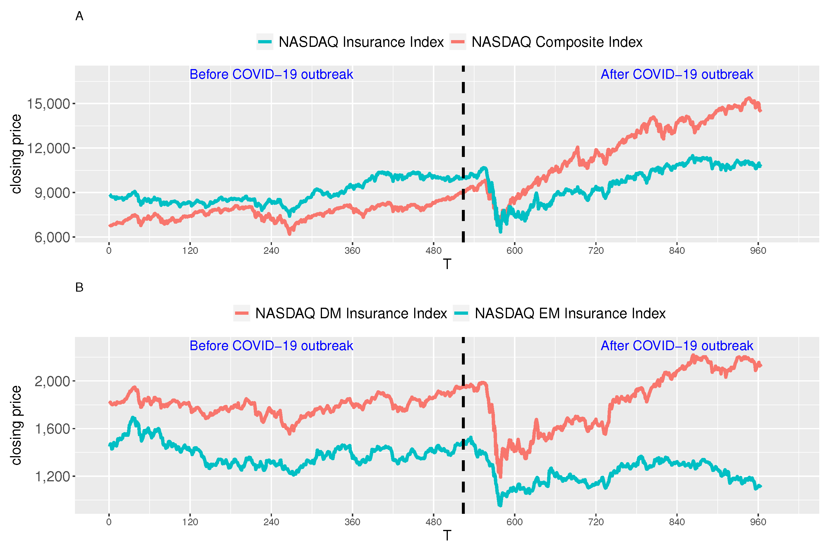
The daily closing prices of the NASDAQ Insurance Index, NASDAQ Developed Markets Insurance Index, NASDAQ Emerging Markets Insurance Index, and NASDAQ Composite Index before and after the occurrence of COVID-19 are illustrated in Figure 1. It is clearly shown that there exist sharp reductions in four series after the occurrence of COVID-19. The contractions of the NASDAQ insurance stock indexes reach the bottom of the series. Before the March 2020 crash, the NASDAQ Insurance Index was larger than the NASDAQ Composite Index. However, after the March 2020 crash, the phenomenon is totally different, the “scissors difference” is observed in Figure 1A.
For the purpose of comparing the multifractality of the different indexes, the logarithmic index values are utilized in the study. The INS Index, DM-INS Index, EM-INS Index, and COMP Index are calculated from the logarithmic values of the NASDAQ Insurance Index, NASDAQ Developed Markets Insurance Index, NASDAQ Emerging Markets Insurance Index, and NASDAQ Composite Index, representing the insurance market, the developed insurance market, the developing insurance market, and the benchmark of the whole market, respectively. Table 1 shows the descriptive statistics of four series.
In order to test the stationarity of the daily INS Index, DM-INS Index, EM-INS Index, and COMP Index, the KPSS (Kwiatkowski Philipps Schmidt Shin) test [33] is utilized and the results are shown in Table 2. Table 2 reports that the four time series reject the null hypothesis, suggesting that these four indexes before and after the occurrence of COVID-19 are nonstationary.

3. Multifractal Analysis

3.1. MF-DFA Method

Consider the time series { x i } = { x 1 , x 2 , , x N } ; the MF-DFA method can be expressed as five steps.
(1) Compute the profile of { x i } :
X i = k = 1 i ( x k x ¯ ) , i = 1 , , N
where x ¯ = 1 N i = 1 N x i .
(2) Subdivide the profile into N s = int ( N / s ) segments that do not overlap with the same length s. Due to the length, N might not be an integer multiple of s, and a short portion of X i might be disregarded at the end. To include this part, repeat the procedure from the other side. Then, 2 N s segments are obtained.
(3) Compute the local trend of every segment through a least-square fitting process. Then, the variance is defined by
V a r s v = 1 s i = 1 s { x ( v 1 ) s + i x i v } 2 , if v = 1 , , N s . 1 s i = 1 s { x ( N ( v N s ) s + i x i v } 2 , if v = N s + 1 , , 2 N s
where x i v is the fitting polynomial in segment v.
(4) Average entire segments to obtain the qth-order fluctuation function:
F q ( s ) = 1 2 N s v = 1 2 N s ( V a r s v ) q / 2 1 / q , if q 0 . exp 1 4 N s v = 1 2 N s ln ( V a r s v ) , if q = 0 .
Repeat steps (2) to (4) with different s to determine how s affects the dependency of F q ( s ) on q.
(5) Investigate the log–log plots F q ( s ) versus s for different q. For long-range power-law correlated series, as s increases, the generalized Hurst exponent H ( q ) can be determined as
F q ( s ) s H ( q ) .
When H ( q ) depending on q is observed, the time series shows multifractality. When H ( q ) is equal on different q, the series is monofractal. Specifically, H ( 2 ) > 0.5 indicates that the series is long-range correlated, which means an increase (decrease) will more possibly show up in succession with another increase (decrease). H ( 2 ) < 0.5 means the series are long-range anti-correlated, which indicates an increase (decrease) will more possibly show up in succession with another decrease (increase). The range of H ( q ) , Δ H = H ( min ( q ) ) H ( max ( q ) ) , determines the extent to which the series is multifractal. Higher Δ H indicates stronger multifractality. In addition, the scaling exponent τ ( q ) is determined as
τ ( q ) = q H ( q ) 1
Via Legendre transform, the singularity strength α and the multifractal spectrum f ( α ) can be calculated by
α = d τ q d q = H ( q ) + q H ( q )
f ( α ) = q α τ ( q ) = 1 + q [ α H ( q ) ]
Multifractal spectrum f ( α ) defines the fractal dimension of the ensemble formed by all the points that share the same singularity exponent α . Fractal dimension f ( α ) α is of a bell shape. The multifractal spectrum width Δ α = max ( α ) min ( α ) measures the degree of the multifractality property. The greater the Δ α value is, the greater the degree of multifractality will be.

3.2. Multifractal Causes Analysis

It is traditionally shown that the causes of multifractality in time series are fat-tailed probability distributions and/or long-range temporal correlations [10]. More recent researches suggest that sources of the multifractality in series may be generated from long-range nonlinear autocorrelations, the fat tails in probability distributions, or linear autocorrelations [34]. However, numerous studies demonstrate that spurious multifractality may present in the series made from monofractal models and mathematical models [35,36]. The linear correlation or long memory in series alone is not sufficient to produce multifractality [37]. The nonlinear correlations in time series are the genuine causes of the multifractality [38,39]. Whether the measured multifractality determined by the traditional methods is intrinsic or apparent and what are the causes of the multifractality in data are significant issues that have attracted the interest of numerous researchers [13,34,38,39,40,41].
To calculate the sources of apparent multifractality, the width of the original time series’ multifractal spectrum Δ α can be broken down into three parts, including the nonlinear correlation Δ α N L , linear correlation Δ α L M , and fat-tailed probability distribution Δ α P D F [13,41,42]. After simulating 10,000 times, Δ α can be expressed as
Δ α = E Δ α N L + E Δ α L M + E Δ α P D F .
Moreover, the shuffling and surrogate procedures are utilized to decompose three components of apparent multifractality. In the surrogate procedure, the improved, amplitude-adjusted Fourier transform (IAAFT) algorithm [43] is applied. A more convenient method, incorporating linear correlations into randomly generated time series derived from the original time series, has been utilized in the construction of the surrogate time series. The width of the multifractal spectrum of surrogate time series can be composed of the linear correlation and the fat-tailed probability distribution [13,44]. The equations of the three components can be described as
E Δ α P D F = E Δ α s h u f .
E Δ α L M = E Δ α s u r r E Δ α P D F .
E Δ α N L = Δ α E Δ α s u r r .
The intrinsic multifractality Δ α I N T R is described as
E Δ α I N T R = E Δ α N L .
Based on Equation (11), the intrinsic multifractality is also described as
E Δ α I N T R = Δ α E Δ α s u r r .
The portion of the intrinsic to apparent multifractality is described as
E INTR ratio = E Δ α I N T R / Δ α .
Then, the multifractal causes analysis based on the employed stochastic simulation (MCASS) can be described as five steps:
Step1 
Shuffle the original series to get rid of any possible correlations. Determine the multifractal characteristics, H s h u f ( q ) and Δ α s h u f , utilizing the MF-DFA analysis.
Step2 
Employ the IAAFT algorithm to phase-randomize the original series to generate the surrogate series. Calculate the multifractal characteristics H s u r r ( q ) and Δ α s u r r .
Step3 
Repeat steps 1–2 10,000 times for each index. The 80,000 sets of { H s h u f ( q ) , H s u r r ( q ) , Δ α s h u f , Δ α s u r r } of the daily INS Index, DM-INS Index, EM-INS Index, and COMP Index before and after the occurrence of COVID-19 are obtained.
Step4 
Calculate the difference among H s h u f ( q ) , H s u r r ( q ) , Δ α s h u f , Δ α s u r r to obtain three parts and intrinsic multifractality of the daily INS Index, DM-INS Index, EM-INS Index, and COMP Index before and after the occurrence of COVID-19, respectively.
Step5 
Compare the above multifractality characteristics to determine the dynamic effects of the COVID-19 epidemic on the intrinsic multifractality of the daily INS Index, DM-INS Index, EM-INS Index, and COMP Index.

3.3. Multifractal Features of INS Index, DM-INS Index, EM-INS Index, and COMP Index

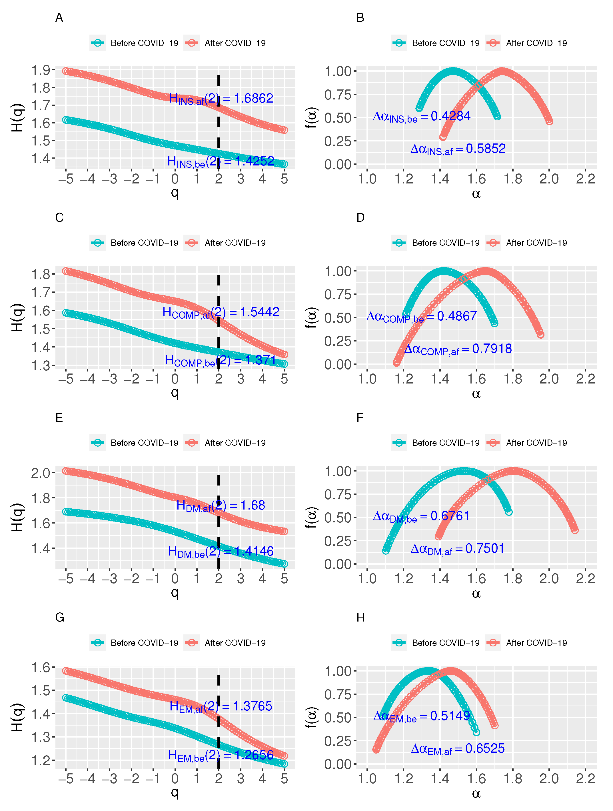
By employing the MF-DFA analysis, the generalized Hurst exponents and the multifractal spectra of the daily INS Index, DM-INS Index, EM-INS Index, and COMP Index before and after the occurrence of COVID-19 are illustrated in Figure 2.
Figure 2A shows that both H I N S , b e ( q ) and H I N S , a f ( q ) vary as q changes, indicating that H ( q ) depends on q and the daily INS Index before and after the occurrence of COVID-19 have a multifractal structure. Furthermore, H I N S , b e ( q ) and H I N S , a f ( q ) decrease as q increases. When q = 2 , H I N S , b e ( 2 ) = 1.4252 > 1 and H I N S , a f ( 2 ) = 1.6862 > 1 show the indexes are long-range correlated, which indicate larger (smaller) values followed by a high possibility. H I N S , a f ( 2 ) > H I N S , b e ( 2 ) shows that there are stronger multifractal characteristics after the COVID-19 outbreak.
Furthermore, Figure 2B shows that the multifractal spectra are of a bell shape, which indicates that the INS Index before and after the occurrence of COVID-19 have multifractal characteristics. Δ α I N S , b e < Δ α I N S , a f shows that greater multifractal degree is obtained after the COVID-19 outbreak.
For the daily DM-INS Index, EM-INS Index, and COMP Index series, the same conclusions can be drawn.
In summary, the daily INS Index, DM-INS Index, EM-INS Index, and COMP Index before and after the occurrence of COVID-19 are multifractal and all indexes are long-range correlated. Furthermore, the stronger multifractal characteristics and the greater multifractal degree are shown in all four series after the occurrence of COVID-19.

3.4. Causes of Multifractality

3.4.1. Baseline Results—Causes of Multifractality of INS Index and COMP Index

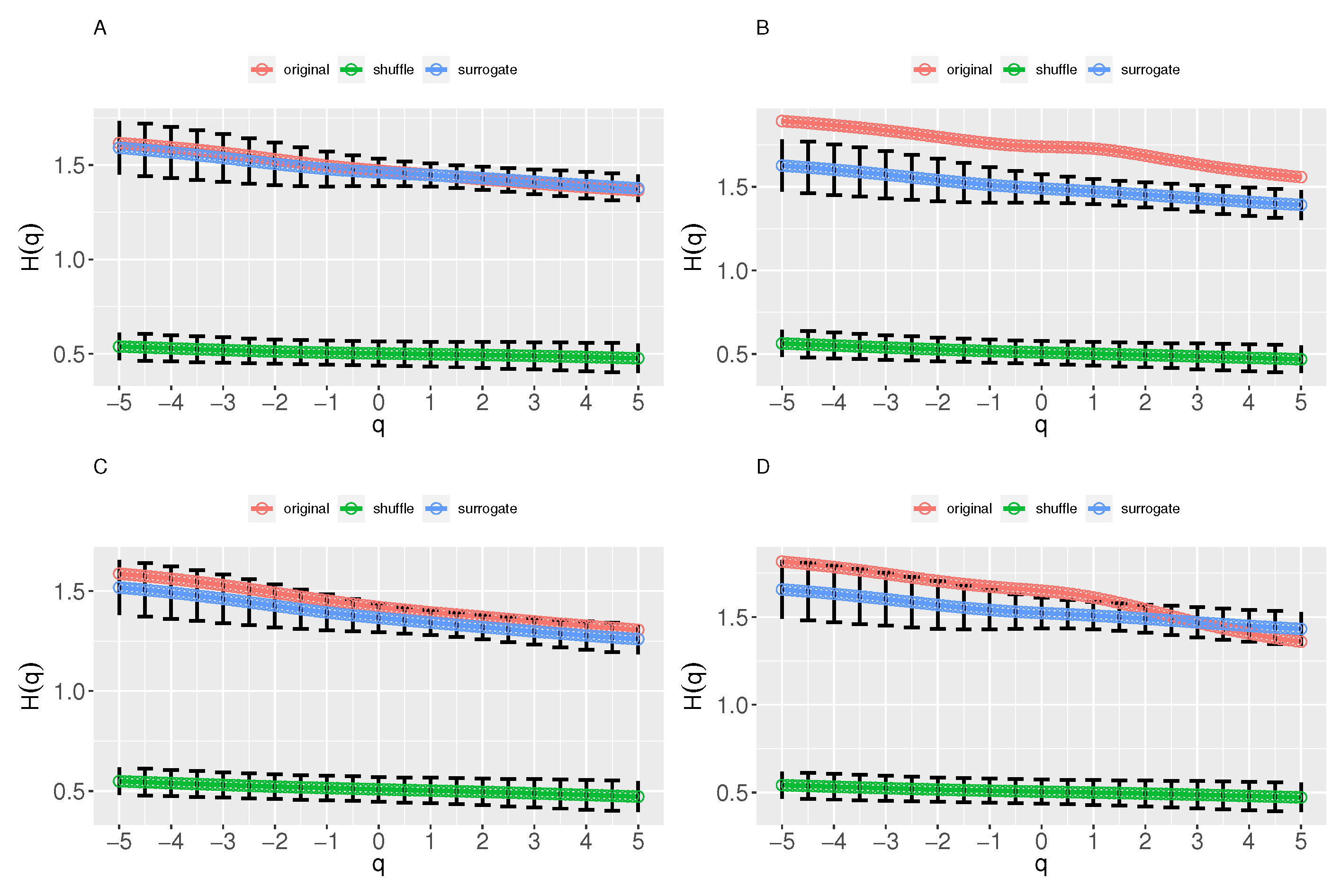
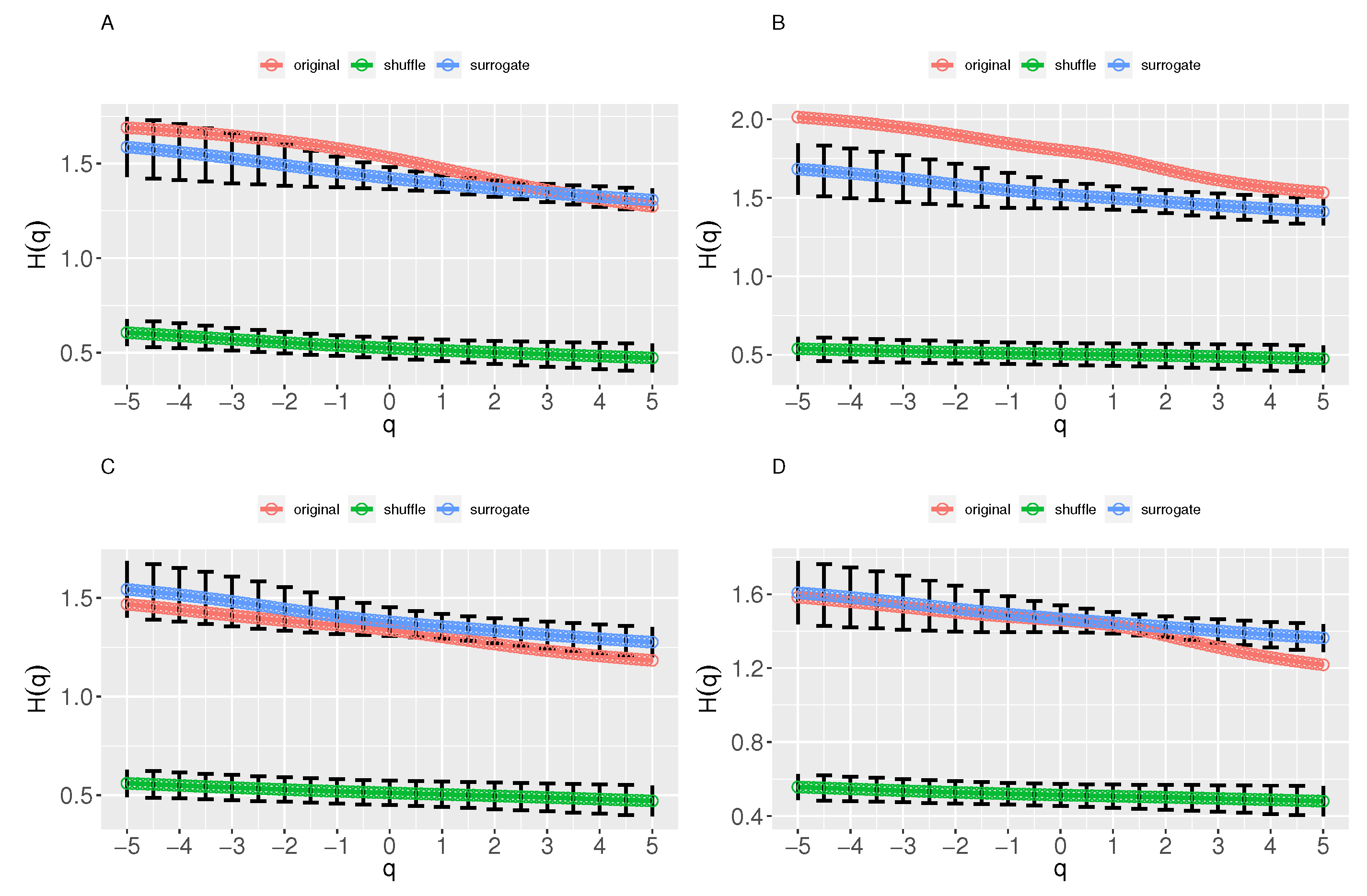
The original daily INS Index and COMP Index before and after the occurrence of COVID-19 are shuffled and phase-randomized 10,000 times, respectively, and the MCASS analysis introduced in Section 3.2 is employed. The generalized Hurst exponents H ( q ) of the shuffled and the surrogate daily INS Index and COMP Index before and after the occurrence of COVID-19 are presented in Figure 3. For the shuffled time series, H I N S , b e s h u f ( q ) , H I N S , a f s h u f ( q ) , H C O M P , b e s h u f ( q ) , and H C O M P , a f s h u f ( q ) are dependent on q and H I N S , b e o r i > H I N S , b e s h u f ( q ) , H I N S , a f o r i ( q ) > H I N S , a f s h u f ( q ) , H C O M P , b e o r i ( q ) > H C O M P , b e s h u f ( q ) , and H C O M P , a f o r i ( q ) > H C O M P , a f s h u f ( q ) hold. It is shown that H I N S , b e s u r r ( q ) , H I N S , a f s u r r ( q ) , H C O M P , b e s u r r ( q ) , and H C O M P , a f s u r r ( q ) are dependent on q and there are small differences between H I N S , b e o r i ( q ) and H I N S , b e s u r r ( q ) , H I N S , a f o r i ( q ) and H I N S , a f s u r r ( q ) , H C O M P , b e o r i ( q ) and H C O M P , b e s u r r ( q ) , and H C O M P , a f o r i ( q ) and H C O M P , a f s u r r ( q ) , respectively.
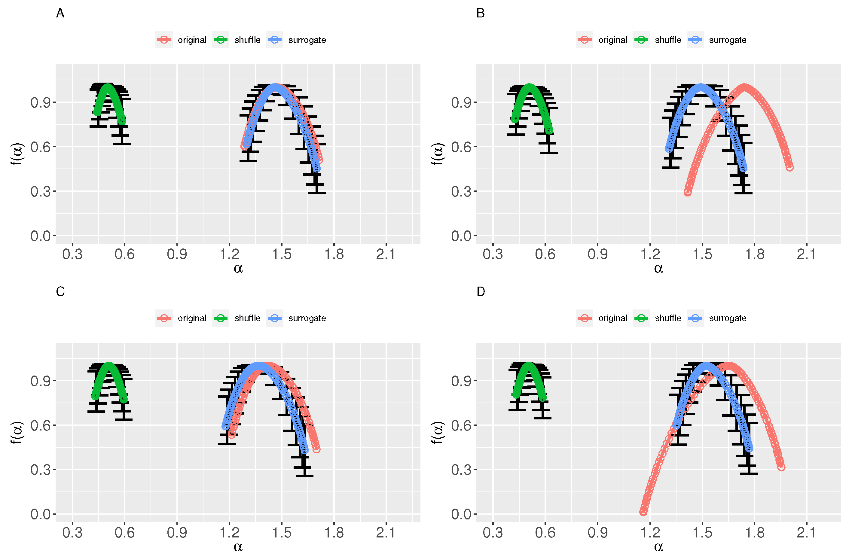
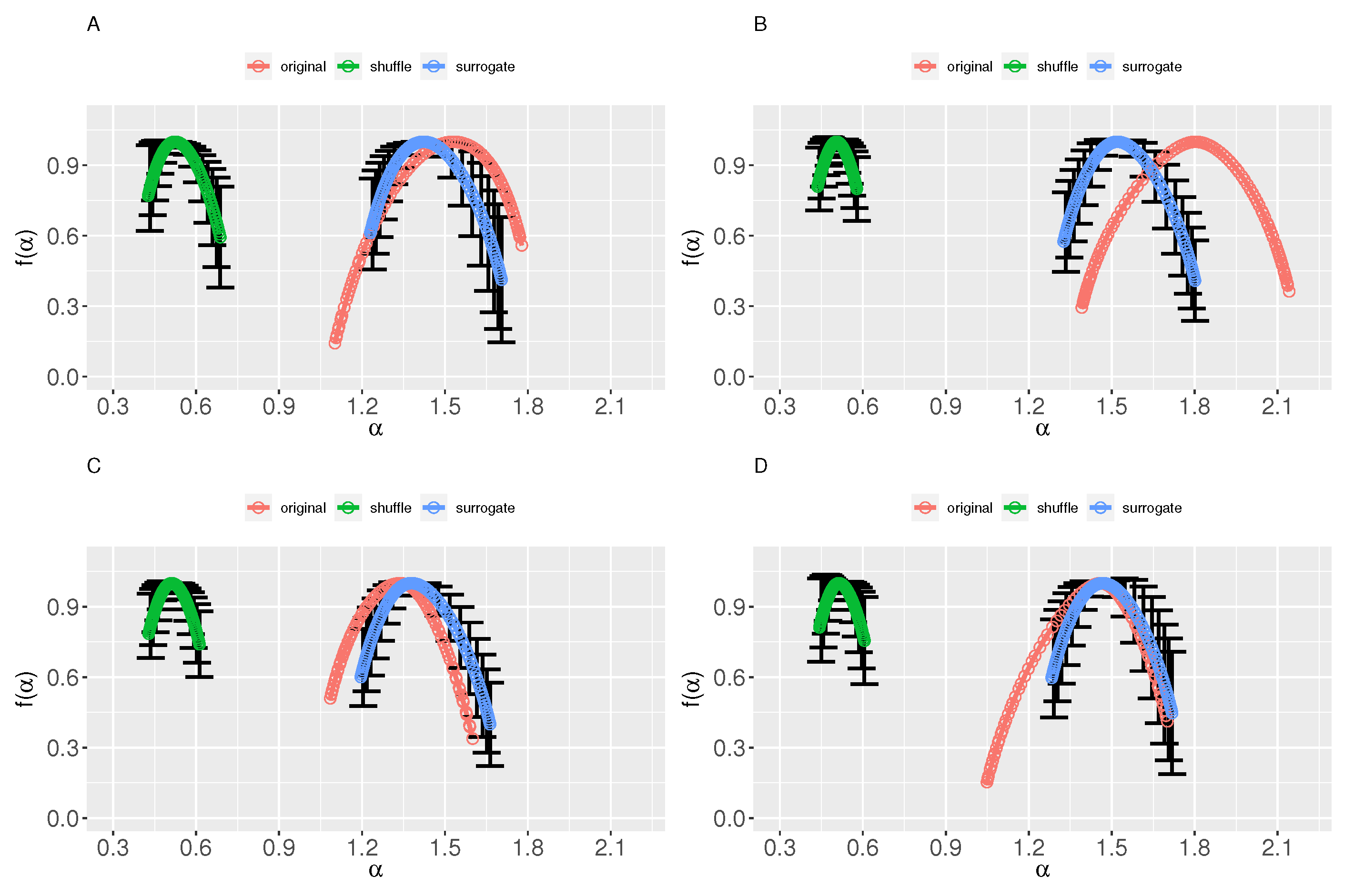
Figure 4 illustrates the multifractal spectra of the shuffled and the surrogate daily INS Index and COMP Index before and after the occurrence of COVID-19 and Table 3 presents the empirical results.
According to Equations (9)–(12), the linear correlation part’s degree of multifractality of the daily INS Index before the occurrence of COVID-19 is Δ α I N S , b e L M = 0.2517 ± 0.1886 . The PDF part’s degree of multifractality is Δ α I N S , b e P D F = 0.1692 ± 0.0867 . The nonlinear correlation part’s degree of multifractality is Δ α I N S , b e N L = 0.0075 ± 0.1678 . The intrinsic multifractality of the daily INS Index before the occurrence of COVID-19 is Δ α I N S , b e I N T R = 0.0075 ± 0.1678 . Analogously, the multifractal components of the INS Index after the occurrence of COVID-19 and the COMP Index before and after the occurrence of COVID-19 can be obtained, which are presented in Table 4.
Table 4 reports that E (INTR ratio I N S , a f ) > E ( INTR ratio I N S , b e ) and E ( INTR ratio C O M P , a f ) > E ( INTR ratio C O M P , b e ) hold, which means the greater intrinsic multifractal degree are obtained after COVID-19 outbreak.

3.4.2. Robustness Test—Causes of Multifractality of DM-INS Index and EM-INS Index

To ensure the robustness of the above conclusions, the robustness tests based on sample restriction are conducted. The baseline conclusions might be originated from companies with particular characteristics and/or in particular areas. Then, tests on the restricted samples are performed to determine whether the conclusions are driven by some specific subsamples. By construction, the DM-INS Index is composed of stocks limited in developed markets and the EM-INS Index is limited in emerging markets. The MCASS analysis introduced in Section 3.2 is repeated in the DM-INS Index and the EM-INS Index to test the robustness.
The generalized Hurst exponents H ( q ) of the shuffled and the surrogate DM-INS Index and the EM-INS Index are illustrated in Figure 5. H D M , b e s h u f ( q ) , H D M , a f s h u f ( q ) , H E M , b e s h u f ( q ) , H E M , a f s h u f ( q ) , H D M , b e s u r r ( q ) , H D M , a f s u r r ( q ) , H E M , b e s u r r ( q ) , and H E M , a f s u r r ( q ) are dependent on q, and H D M , b e o r i ( q ) > H D M , b e s h u f ( q ) , H D M , a f o r i ( q ) > H D M , a f s h u f ( q ) , H E M , b e o r i ( q ) > H E M , b e s h u f ( q ) , and H E M , a f o r i ( q ) > H E M , a f s h u f ( q ) hold. There are small differences between H D M , b e o r i ( q ) and H D M , b e s u r r ( q ) , H D M , a f o r i ( q ) and H D M , a f s u r r ( q ) , H E M , b e o r i ( q ) and H E M , b e s u r r ( q ) , and H E M , a f o r i ( q ) and H E M , a f s u r r ( q ) , respectively.
The multifractal spectra of the shuffled and the surrogate DM-INS Index and EM-INS Index are presented in Figure 6 and Table 5. The components and intrinsic multifractality of the DM-INS Index and EM-INS Index before and after the occurrence of COVID-19 are listed in Table 6. E (INTR ratio D M , a f ) > E ( INTR ratio D M , b e ) , E (INTR ratio E M , a f ) > E ( INTR ratio E M , b e ) means the greater intrinsic multifractal degrees are obtained after COVID-19 outbreak. All the above conclusions are similar to baseline results.

4. Multifractal Cross-Correlation Analysis

In this section, the dynamic effects of the COVID-19 epidemic on the multifractal cross-correlation of the pair of series, the NASDAQ Composite Index and NASDAQ Insurance Index time, before and after the occurrence of COVID-19 are analyzed.

4.1. MF-DCCA Method

Consider two time series { x i } = { x 1 , x 2 , , x N } and { y i } = { y 1 , y 2 , , y N } ; the MF-DCCA method can be expressed as five steps.
(1) Calculate the profiles of { x i } and { y i } :
X i = k = 1 i ( x k x ¯ ) , i = 1 , , N , Y i = k = 1 i ( y k y ¯ ) , i = 1 , , N ,
where x ¯ = 1 N i = 1 N x i and y ¯ = 1 N i = 1 N y i .
(2) Subdivide the profile into N s = int ( N / s ) bins that do not overlap with the same length of s. Considering N might not be a multiple of s, a short portion of the series might be left. To contain this part, repeat the same process from the other side. So, 2 N s bins are obtained.
(3) Fit each bin utilizing the least square method; the cross-correlation can be obtained by
V a r s v = 1 s i = 1 s [ X i v X ˜ i v ] 2 × [ Y i v Y ˜ i v ] 2 q / 4
where X ˜ i v and Y ˜ i v is the fitting polynomial in segment v.
(4) The qth-order fluctuation function can be determined by
F x / y ( q , s ) = 1 2 N s v = 1 2 N s ( V a r s v ) 1 / q , if q 0 . 1 2 F x / y ( 1 , s ) + F x / y ( 1 , s ) , if q = 0 .
Steps (2) to (4) are repeated for different values of s.
(5) The generalized Hurst exponent H x / y ( q ) would present power law structure when the series show long-range power-law correlation characteristics:
F x / y ( q , s ) s H x / y ( q ) .
If H x / y ( q ) does not depend on q, the cross-correlation between two series is monofractal. When H x / y ( q ) depends on q, the cross-correlation between two series is multifractal. The range of H x / y ( q ) , Δ H x / y = H x / y ( min ( q ) ) H x / y ( max ( q ) ) , illustrates the extent of multifractal cross-correlation. The scaling exponent τ x / y ( q ) can be described as
τ x / y ( q ) = q H x / y ( q ) 1
The singularity strength α x / y and the multifractal spectrum f x / y ( α ) can be described as
α x / y = d τ x / y q d q = H x / y ( q ) + q H x / y ( q )
f x / y ( α x / y ) = q α x / y ( q ) τ x / y ( q ) = 1 + q [ α x / y H x / y ( q ) ]
The width of multifractal spectrum Δ α x / y = max ( α x / y ) min ( α x / y ) indicates the degree of the multifractal cross-correlation.

4.2. Multifractal Cross-Correlation of INS/COMP

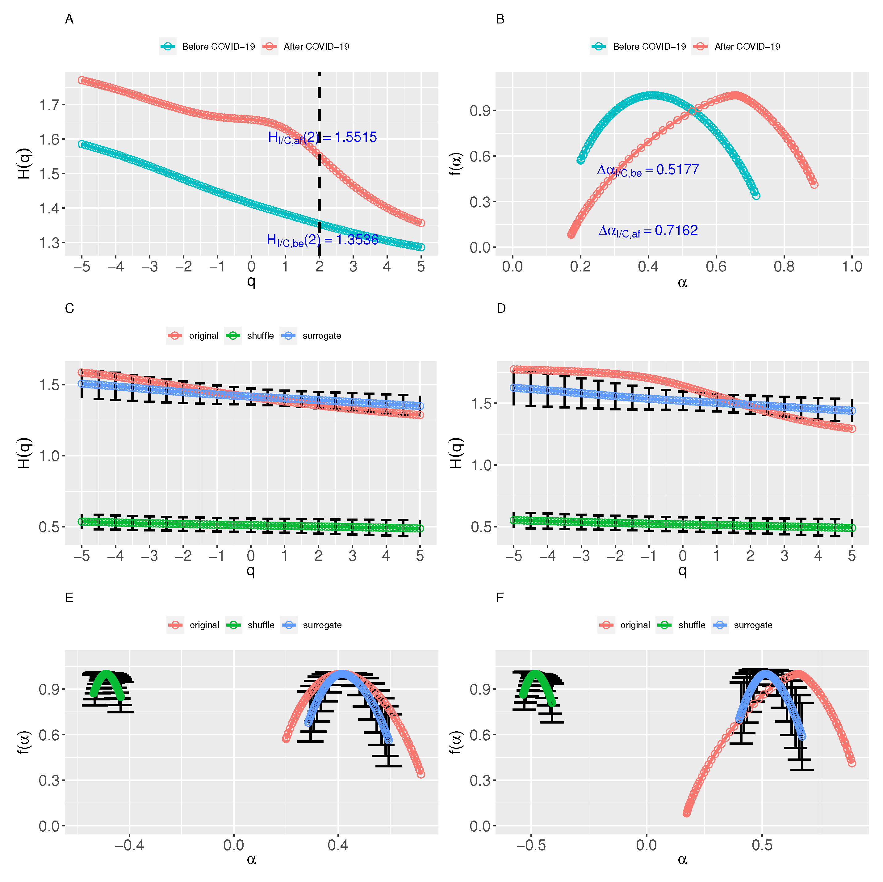
To determine the cross-correlation of INS/COMP before and after the occurrence of COVID-19, the MF-DCCA method is employed to compute the generalized Hurst exponents and the multifractal spectra. The values are shown in Figure 7.
Figure 7A,B show that the cross-correlation of daily INS/COMP before and after the occurrence of COVID-19 are multifractal. The stronger multifractal cross-correlation and greater multifractal cross-correlation degree after the occurrence of COVID-19 are obtained.

4.3. Causes of Cross-Correlation of INS/COMP

Similar to the multifractal causes analysis in Section 3.2, to calculate the components of apparent multifractal cross-correlations, the width of the original series’ multifractal spectrum Δ α x / y can be broken down to the nonlinear correlation part Δ α x / y N L , linear correlation part Δ α x / y L M , and fat-tailed probability distribution part Δ α x / y P D F [41,42]. By integrating the simulation 10,000 times, Δ α x / y is described as
Δ α x / y = E Δ α x / y N L + E Δ α x / y L M + E Δ α x / y P D F .
Moreover, the shuffling and the IAAFT surrogate process are employed to break down the apparent multifractality. The components can be described as.
E Δ α x / y P D F = E Δ α x / y s h u f .
E Δ α x / y L M = E Δ α x / y s u r r E Δ α x / y P D F .
E Δ α x / y N L = Δ α x / y E Δ α x / y s u r r .
The intrinsic multifractal cross-correlation Δ α x / y I N T R is described as
E Δ α x / y I N T R = E Δ α x / y N L .
Based on Equation (25), the intrinsic multifractal cross-correlation is also described as
E Δ α x / y I N T R = Δ α x / y E Δ α x / y s u r r .
The portion of the intrinsic to apparent multifractal cross-correlation is described as
E INTR ratio x / y = E Δ α x / y I N T R / Δ α x / y .
Further to Section 3.2, the MCASS analysis can be extended to the multifractal cross-correlations causes analysis. The main difference is to substitute the MF-DFA analysis with the MF-DCCA analysis.
After shuffling and phase-randomizing the original pair (INS/COMP) before and after the occurrence of COVID-19 10,000 times, the multifractal cross-correlation causes analysis is employed. The generalized Hurst exponents H x / y ( q ) of the shuffled and the surrogate INS/COMP before and after the occurrence of COVID-19 are described in Figure 7C–F and Table 7.
Based on Equation (26), the multifractal components of INS/COMP before COVID-19 outbreak can be obtained: Δ α I / C , b e L M = 0.2061 ± 0.1573 , Δ α I / C , b e P D F = 0.1223 ± 0.0624 , Δ α I / C , b e N L = 0.1893 ± 0.1412 . The intrinsic multifractal cross-correlation is Δ α I / C , b e I N T R = 0.1893 ± 0.1412 . Analogously, the multifractal components of INS/COMP after the occurrence of COVID-19 can be obtained. Table 8 presents the results.
E (INTR ratio I / C , a f ) > E ( INTR ratio I / C , b e ) shows that the contribution of the intrinsic multifractal cross-correlation of daily INS/COMP increases after the COVID-19 outbreak.

4.4. Discussion

The nonlinear correlation part is the genuine source of the multifractality among three parts [38,39] and indicates that the apparent multifractality and multifractal cross-correlation might overestimate. Table 9 shows the change ratios of apparent and intrinsic multifractality.
The change ratios of apparent and intrinsic multifractality of all four series increased, indicating that the larger multifractality degrees are obtained after the occurrence of COVID-19 and the March 2020 crash. Similar results are found in previous multifractal behavior research. Los C.A. and Yalamova R. found that the 1987 financial crisis contributed to the changes in the multifractal spectra, indicating an increased complexity [30]. Caraiani P. illustrated that the crisis had impacted the multifractal spectrum during the 2008 crisis [22].
Furthermore, the results illustrate that although the COVID-19 and the March 2020 crash contribute to the increase of multifractality of the four series, their effects on intrinsic multifractality are limited.
Among the four series, the intrinsic multifractality of the NASDAQ Insurance Index, the NASDAQ Emerging Markets Insurance Index, and the NASDAQ Composite Index series ascend largely (more than 20%). The change ratios of the intrinsic multifractality of the NASDAQ Composite Index are the maximum, meaning the insurance stock markets are less affected by such crashes than the benchmark of the whole stock markets.
Moreover, the change ratios of the intrinsic multifractality of the NASDAQ Emerging Markets Insurance Index are larger than those of the NASDAQ Developed Markets Insurance Index, indicating that the emerging insurance markets are more affected by such incidents than the developed insurance markets. Similar conclusions are reported in the study of COVID-19 impact on insurance firms. Farooq et al. examined the abnormal returns of 958 insurance companies and found that COVID-19 negatively affected the stock returns, particularly in the case of insurance firms operating in developing countries [9].

5. Conclusions

Triggered by the COVID-19 epidemic, the global economy has been significantly, adversely affected. In this study, the dynamic effects of the COVID-19 epidemic on the multifractality of NASDAQ insurance stock markets are examined. First of all, the multifractal features, multifractal causes analysis, and dynamic effects of the COVID-19 epidemic on multifractality of the daily INS Index, DM-INS Index, EM-INS Index, and COMP Index, representing the insurance market, developed insurance market and developing insurance market, and the whole market are investigated. Moreover, the multifractal cross-correlation, components of the multifractality, and dynamic effects of the COVID-19 epidemic on the cross-correlation of the pair of series, the INS/COMP, are illustrated. The conclusions are summed up as follows:
(1)
The NASDAQ Insurance Index, Developed Markets Insurance Index, Emerging Markets Insurance Index, and NASDAQ Composite Index series both before and after the occurrence of COVID-19 are multifractal and long-range correlated. Furthermore, the stronger multifractal characteristics and the greater multifractal degree are shown in all four series after the occurrence of COVID-19.
(2)
The contribution of the intrinsic multifractality of four series increases after the occurrence of COVID-19. The intrinsic multifractality of the NASDAQ Insurance Index, Emerging Markets Insurance Index, and NASDAQ Composite Index series ascend largely.
(3)
The cross-correlations between the NASDAQ Insurance Index and the NASDAQ Composite Index series both before and after the occurrence of COVID-19 are multifractal. There are stronger multifractal cross-correlations and greater multifractal degrees between the pair of series after the occurrence of COVID-19. The contribution of the intrinsic multifractal cross-correlation increases after the occurrence of COVID-19.
(4)
Although COVID-19 and the March 2020 crash contribute to the increase of multifractality of four series, their effects on intrinsic multifractality are limited. The intrinsic multifractality of the NASDAQ Insurance Index, the NASDAQ Emerging Markets Insurance Index, and the NASDAQ Composite Index series ascend largely. The insurance stock markets are less affected by such crashes than the benchmark of the whole stock market. The emerging insurance markets are more affected by such incidents than the developed insurance markets.
Therefore, the dynamic analysis of the multifractality of the NASDAQ insurance markets and cross-correlations between the NASDAQ insurance market/the whole market before and after the COVID-19 epidemic provide perspectives and a deeper comprehension of the complexity of NASDAQ insurance stock markets. These findings are helpful in providing objective direction and reliable support for decision-making for policymakers, regulators, and investors in the insurance industry in the aftermath of the COVID-19 epidemic.

Author Contributions

Conceptualization, X.L.; validation, X.L. and F.S.; methodology, X.L.; investigation, X.L. and F.S.; software, X.L.; formal analysis, X.L.; data curation, X.L; writing—original draft preparation, X.L; visualization, X.L.; writing—review and editing, X.L. and F.S. All authors have read and agreed to the published version of the manuscript.

Funding

This research received no external funding.

Data Availability Statement

Not applicable.

Conflicts of Interest

The authors declare no conflict of interest.

References

  1. Global Economic Prospects; World Bank: Washington, DC, USA, 2021.
  2. Lan, C.; Huang, Z.; Huang, W. Systemic risk in China’s financial industry due to the COVID-19 pandemic. Asian Econ. Lett. 2020, 1, 18070. [Google Scholar] [CrossRef]
  3. Foglia, M.; Addi, A.; Wang, G.; Angelini, E. Bearish Vs Bullish risk network: A Eurozone financial system analysis. J. Int. Financ. Mark. Inst. Money 2022, 77, 101522. [Google Scholar] [CrossRef]
  4. Caporale, G.M.; Cerrato, M.; Zhang, X. Analysing the determinants of insolvency risk for general insurance firms in the UK. J. Bank. Financ. 2017, 84, 107–122. [Google Scholar] [CrossRef]
  5. Sharpe, I.G.; Stadnik, A. Financial distress in Australian general insurers. J. Risk Insur. 2007, 74, 377–399. [Google Scholar] [CrossRef]
  6. Baluch, F.; Stanley, M.; Chris, P. Insurance, systemic risk and the financial crisis. Geneva Pap. Risk Insur.-Issues Pract. 2011, 36, 126–163. [Google Scholar] [CrossRef] [Green Version]
  7. Drake, P.P.; Neale, F.R.; Schorno, P.J.; Semaan, E. Risk During the Financial Crisis: The Role of the Insurance Industry. J. Insur. Issues 2017, 40, 181–214. [Google Scholar]
  8. Babuna, P.; Yang, X.; Gyilbag, A.; Awudi, D.A.; Ngmenbelle, D.; Bian, D. The Impact of COVID-19 on the Insurance Industry. Int. J. Environ. Res. Public Health 2020, 17, 5766. [Google Scholar] [CrossRef]
  9. Farooq, U.; Nasir, A.; Bilal; Quddoos, M.U. The impact of COVID-19 pandemic on abnormal returns of insurance firms: A cross-country evidence. Appl. Econ. 2021, 53, 3658–3678. [Google Scholar] [CrossRef]
  10. Kantelhardt, J.W.; Zschiegner, S.A.; Koscielny-Bunde, E.; Havlin, S.; Bunde, A.; Stanley, H. Multifractal detrended fluctuation analysis of nonstationary time series. Phys. A Stat. Mech. Its Appl. 2002, 316, 87–114. [Google Scholar] [CrossRef] [Green Version]
  11. Shang, P.; Lu, Y.; Kamae, S. Detecting long-range correlations of traffic time series with multifractal detrended fluctuation analysis. Chaos Solitons Fractals 2008, 36, 82–90. [Google Scholar] [CrossRef]
  12. Laib, M.; Golay, J.; Telesca, L.; Kanevskia, M. Multifractal analysis of the time series of daily means of wind speed in complex regions. Chaos Solitons Fractals 2018, 109, 118–127. [Google Scholar] [CrossRef]
  13. Li, X. On the multifractal analysis of air quality index time series before and during COVID-19 partial lockdown: A case study of Shanghai, China. Phys. A Stat. Mech. Its Appl. 2021, 565, 125551. [Google Scholar] [CrossRef] [PubMed]
  14. Oświe¸cimka, P.; Kwapień, J.; Drożdż, S. Multifractality in the stock market: Price increments versus waiting times. Phys. A Stat. Mech. Its Appl. 2005, 347, 626–638. [Google Scholar] [CrossRef] [Green Version]
  15. Tiwari, A.K.; Albulescu, C.T.; Yoon, S.M. A multifractal detrended fluctuation analysis of financial market efficiency: Comparison using Dow Jones sector ETF indices. Phys. A Stat. Mech. Its Appl. 2017, 483, 182–192. [Google Scholar] [CrossRef]
  16. El Alaoui, M. Price–volume multifractal analysis of the Moroccan stock market. Phys. A Stat. Mech. Its Appl. 2017, 486, 473–485. [Google Scholar] [CrossRef]
  17. Aslam, F.; Aziz, S.; Nguyen, D.K.; Mughal, K.S.; Khan, M. On the efficiency of foreign exchange markets in times of the COVID-19 pandemic. Technol. Forecast. Soc. Chang. 2020, 161, 120261. [Google Scholar] [CrossRef]
  18. Mensi, W.; Lee, Y.J.; Al-Yahyaee, K.H.; Sensoy, A.; Yoon, S.M. Intraday downward/upward multifractality and long memory in Bitcoin and Ethereum markets: An asymmetric multifractal detrended fluctuation analysis. Financ. Res. Lett. 2019, 31, 19–25. [Google Scholar] [CrossRef]
  19. Mnif, E.; Jarboui, A.; Mouakhar, K. How the cryptocurrency market has performed during COVID 19? A multifractal analysis. Financ. Res. Lett. 2020, 36, 101647. [Google Scholar] [CrossRef]
  20. Zhou, W.X. Multifractal detrended cross-correlation analysis for two nonstationary signals. Phys. Rev. E 2008, 77, 066211. [Google Scholar] [CrossRef] [Green Version]
  21. Cao, G.; Xu, L.; Cao, J. Multifractal detrended cross-correlations between the Chinese exchange market and stock market. Phys. A Stat. Mech. Its Appl. 2012, 391, 4855–4866. [Google Scholar] [CrossRef]
  22. Caraiani, P. Evidence of multifractality from emerging European stock markets. PLoS ONE 2012, 7, e40693. [Google Scholar] [CrossRef] [PubMed]
  23. Ma, F.; Wei, Y.; Huang, D. Multifractal detrended cross-correlation analysis between the Chinese stock market and surrounding stock markets. Phys. A Stat. Mech. Its Appl. 2013, 392, 1659–1670. [Google Scholar] [CrossRef]
  24. Ruan, Q.; Zhang, S.; Lv, D.; Lu, X. Financial liberalization and stock market cross-correlation: MF-DCCA analysis based on Shanghai-Hong Kong Stock Connect. Phys. A Stat. Mech. Its Appl. 2018, 491, 779–791. [Google Scholar] [CrossRef]
  25. Zhang, X.; Yang, L.; Zhu, Y. Analysis of multifractal characterization of Bitcoin market based on multifractal detrended fluctuation analysis. Phys. A Stat. Mech. Its Appl. 2019, 523, 973–983. [Google Scholar] [CrossRef]
  26. He, L.Y.; Chen, S.P. Multifractal Detrended Cross-Correlation Analysis of agricultural futures markets. Chaos Solitons Fractals 2011, 44, 355–361. [Google Scholar] [CrossRef]
  27. Zhang, S.; Guo, Y.; Cheng, H.; Zhang, H. Cross-correlations between price and volume in China’s crude oil futures market: A study based on multifractal approaches. Chaos Solitons Fractals 2021, 144, 110642. [Google Scholar] [CrossRef]
  28. Jiang, Z.Q.; Zhou, W.X. Direct Evidence for Inversion Formula in Multifractal Financial Volatility Measure. Chin. Phys. Lett. 2009, 26, 293–296. [Google Scholar]
  29. Dai, M.; Hou, J.; Gao, J.; Su, W.; Xi, L. Mixed multifractal analysis of China and US stock index series. Chaos Solitons Fractals 2016, 87, 268–275. [Google Scholar] [CrossRef]
  30. Los, C.A.; Yalamova, R.M. Multifractal spectral analysis of the 1987 stock market crash. Int. Res. J. Financ. Econ. 2006, 1, 106–133. [Google Scholar]
  31. Yalamova, R. Empirical testing of multifractality of financial time series based on WTMM. Fractals-Complex Geom. Patterns Scaling Nat. Soc. 2009, 17, 323–332. [Google Scholar] [CrossRef]
  32. Siokis, F.M. Financial markets during highly anxious time: Multifractal fluctuations in asset returns. Fractals-Complex Geom. Patterns Scaling Nat. Soc. 2017, 25, 1750032. [Google Scholar] [CrossRef]
  33. Kwiatkowski, D.; Phillips, P.C.B.; Schmidt, P.; Shin, Y. Testing the null hypothesis of stationarity against the alternative of a unit root. J. Econom. 1992, 54, 159–178. [Google Scholar] [CrossRef]
  34. Rak, R.; Grech, D. Quantitative approach to multifractality induced by correlations and broad distribution of data. Phys. A Stat. Mech. Its Appl. 2018, 508, 48–66. [Google Scholar] [CrossRef]
  35. Bouchaud, J.P.; Potters, M.; Meyer, M. Apparent multifractality in financial time series. Eur. Phys. J. B-Condens. Matter Complex Syst. 2000, 13, 595–599. [Google Scholar] [CrossRef] [Green Version]
  36. von Hardenberg, J.; Thieberger, R.; Provenzale, A. A box-counting red herring. Phys. Lett. A 2000, 269, 303–308. [Google Scholar] [CrossRef]
  37. Saichev, A.; Sornette, D. Generic multifractality in exponentials of long memory processes. Phys. Rev. E 2006, 74, 011111. [Google Scholar] [CrossRef] [Green Version]
  38. Drożdż, S.; Kwapień, J.; Oświecimka, P.; Rak, R. Quantitative features of multifractal subtleties in time series. Europhys. Lett. 2009, 88, 60003. [Google Scholar] [CrossRef] [Green Version]
  39. Buonocorea, R.; Aste, T.; Matteo, T. Measuring multiscaling in financial time-series. Chaos Solitons Fractals 2016, 88, 38–47. [Google Scholar] [CrossRef] [Green Version]
  40. Kwapień, J.; Oświecimka, P.; Drożdż, S. Components of multifractality in high-frequency stock returns. Phys. A Stat. Mech. Its Appl. 2005, 350, 466–474. [Google Scholar] [CrossRef] [Green Version]
  41. Zhou, W.X. Finite-size effect and the components of multifractality in financial volatility. Chaos Solitons Fractals 2012, 45, 147–155. [Google Scholar] [CrossRef] [Green Version]
  42. Jiang, Z.Q.; Xie, W.J.; Zhou, W.X.; Sornetted, D. Multifractal analysis of financial markets: A review. Rep. Prog. Phys. 2019, 82. [Google Scholar] [CrossRef] [PubMed] [Green Version]
  43. Schreiber, T.; Schmitz, A. Improved Surrogate Data for Nonlinearity Tests. Phys. Rev. Lett. 1996, 77, 635. [Google Scholar] [CrossRef] [PubMed] [Green Version]
  44. Chen, F.; Miao, Y.; Tian, K.; Ding, X.; Li, T. Multifractal cross-correlations between crude oil and tanker freight rate. Phys. A Stat. Mech. Its Appl. 2017, 474, 344–354. [Google Scholar] [CrossRef]
Figure 1. The daily closing prices of the four indexes before and after the occurrence of COVID-19. (A) NASDAQ Insurance Index and NASDAQ Composite Index, (B) NASDAQ DM(Developed Markets) Insurance Index and NASDAQ EM(Emerging Markets) Insurance Index.
Fractalfract 07 00091 g001
Figure 2. The generalized Hurst exponents and the multifractal spectra of the daily INS Index (A,B), COMP Index (C,D), DM-INS Index (E,F), and EM-INS Index (G,H) before and after the occurrence of COVID-19.
Fractalfract 07 00091 g002
Figure 3. The generalized Hurst exponents of the shuffled and surrogate daily INS Index and COMP Index before and after the occurrence of COVID-19. (A) INS Index, before COVID-19 outbreak. (B) INS Index, after COVID-19 outbreak. (C) COMP Index, before COVID-19 outbreak. (D) COMP Index, after COVID-19 outbreak. The error bars show the standard deviations for the 10,000 simulations, respectively.
Fractalfract 07 00091 g003
Figure 4. The multifractal spectra of the shuffled and surrogate daily INS Index and COMP Index before and after the occurrence of COVID-19. (A) INS Index, before COVID-19 outbreak. (B) INS Index, after COVID-19 outbreak. (C) COMP Index, before COVID-19 outbreak. (D) COMP Index, after COVID-19 outbreak. The error bars show the standard deviations for the 10,000 simulations, respectively.
Fractalfract 07 00091 g004
Figure 5. The robustness test results. The generalized Hurst exponents of the shuffled and surrogate daily DM-INS Index and EM-INS Index before and after the occurrence of COVID-19. (A) DM-INS Index, before COVID-19 outbreak. (B) DM-INS Index, after COVID-19 outbreak. (C) EM-INS Index, before COVID-19 outbreak. (D) EM-INS Index, after COVID-19 outbreak. The error bars show the standard deviations for the 10,000 simulations, respectively.
Fractalfract 07 00091 g005
Figure 6. The robustness test results. The multifractal spectra of the shuffled and surrogate daily DM-INS Index and EM-INS Index before and after the occurrence of COVID-19. (A) DM-INS Index, before COVID-19 outbreak. (B) DM-INS Index, after COVID-19 outbreak. (C) EM-INS Index, before COVID-19 outbreak. (D) EM-INS Index, after COVID-19 outbreak. The error bars show the standard deviations for the 10,000 simulations, respectively.
Fractalfract 07 00091 g006
Figure 7. The generalized Hurst exponents and the multifractal spectra of the original, shuffled, and surrogate daily INS/COMP before and after the occurrence of COVID-19. (A) Original series, before COVID-19 outbreak. (B) Original series, after COVID-19 outbreak. (C) Generalized Hurst exponents, before COVID-19 outbreak. (D) Generalized Hurst exponents, after COVID-19 outbreak. (E) Multifractal spectra, before COVID-19 outbreak. (F) Multifractal spectra, after COVID-19 outbreak. The error bars show the standard deviations for the 10,000 simulations, respectively.
Fractalfract 07 00091 g007
Table 1. Descriptive statistics of the daily INS Index, DM-INS Index, EM-INS Index, and COMP Index before and after the occurrence of COVID-19.
Time SeriesPeriodMeanStd.MedianMinMaxSkewnessKurtosis
INS Indexbefore COVID-199.10.089.078.919.250.42−1.18
after COVID-199.170.139.218.769.35−0.77−0.37
DM-INS Indexbefore COVID-197.490.047.497.357.58−0.540.6
after COVID-197.510.157.547.087.7−0.48−0.9
EM-INS Indexbefore COVID-197.240.077.237.17.430.52−0.01
after COVID-197.110.097.126.867.330.01−0.31
COMP Indexbefore COVID-198.940.078.958.739.11−0.04−0.3
after COVID-199.360.29.388.839.64−0.53−0.73
Table 2. KPSS tests of the daily INS Index, DM-INS Index, EM-INS Index, and COMP Index before and after the occurrence of COVID-19.
Time SeriesPeriodLevelp-Value
INS Indexbefore COVID-195.35520.01
after COVID-194.69360.01
DM-INS Indexbefore COVID-191.35230.01
after COVID-194.91470.01
EM-INS Indexbefore COVID-191.81230.01
after COVID-190.70700.01
COMP Indexbefore COVID-193.79310.01
after COVID-196.84050.01
Table 3. Comparison of the width of multifractal spectra Δ α of original, shuffled, and surrogate series of daily INS Index and COMP Index before and after the occurrence of COVID-19. The values in parentheses present the standard deviations.
Time SeriesPeriodOriginal SeriesShuffled SeriesSurrogate Series
INS Indexbefore COVID-190.42840.16920.4209
(0.0867)(0.1678)
after COVID-190.58520.21490.4507
(0.1025)(0.1843)
COMP Indexbefore COVID-190.48670.18460.4657
(0.0926)(0.1775)
after COVID-190.79180.1786(0.4484
(0.091)(0.1907)
Table 4. Comparison of the components and intrinsic multifractality of daily INS Index and COMP Index before and after the occurrence of COVID-19. The values in parentheses present the standard deviations.
Time SeriesPeriod Δ α Δ α LM Δ α NL Δ α PDF Δ α INTR INTR Ratio
INS Indexbefore COVID-190.42840.25170.00750.16920.00751.75%
(0.1886)(0.1678)(0.0867)(0.1678)(39.18%)
after COVID-190.58520.23580.13450.21490.134522.98%
(0.2123)(0.1843)(0.1025)(0.1843)(31.49%
COMP Indexbefore COVID-190.48670.28110.02100.18460.0214.31%
(0.1996)(0.1775)(0.0926)(0.1775)(36.47%)
after COVID-190.79180.26980.34340.17860.343443.37%
(0.2109)(0.1907)(0.091)(0.1907)(24.08%)
Table 5. The robustness test results. The comparison of the width of multifractal spectra Δ α of original, shuffled, and surrogate series of daily DM-INS Index and EM-INS Index before and after the occurrence of COVID-19. The values in parentheses present the standard deviations.
Time SeriesPeriodOriginal SeriesShuffled SeriesSurrogate Series
INS Indexbefore COVID-190.42840.16920.4209
(0.0867)(0.1678)
after COVID-190.58520.21490.4507
(0.1025)(0.1843)
DM-INS Indexbefore COVID-190.67610.27430.4895
(0.1271)(0.2031)
after COVID-190.75010.17070.4947
(0.089)(0.1941)
EM-INS Indexbefore COVID-190.51490.20120.4812
(0.0971)(0.1845)
after COVID-190.65250.19560.4625
(0.1047)(0.204)
Table 6. The robustness test results. The comparison of the components of the width of multifractal spectra of daily DM-INS Index and EM-INS Index before and after the occurrence of COVID-19. The values in parentheses present the standard deviations.
Time SeriesPeriod Δ α Δ α LM Δ α NL Δ α PDF Δ α INTR INTR Ratio
INS Indexbefore COVID-190.42840.25170.00750.16920.00751.75%
(0.1886)(0.1678)(0.0867)(0.1678)(39.18%)
after COVID-190.58520.23580.13450.21490.134522.98%
(0.2123)(0.1843)(0.1025)(0.1843)(31.49%)
DM-INS Indexbefore COVID-190.67610.21520.18660.27430.186627.60%
(0.2396)(0.2031)(0.1271)(0.2031)(30.04%)
after COVID-190.75010.3240.25540.17070.255434.05%
(0.2131)(0.1941)(0.089)(0.1941)(25.88%)
EM-INS Indexbefore COVID-190.51490.280.03370.20120.03376.54%
(0.2068)(0.1845)(0.0971)(0.1845)(35.83)%
after COVID-190.65250.26690.19000.19560.1929.12%
(0.231)(0.2040)(0.1047)(0.204)(31.26%)
Table 7. Comparison of the width of multifractal spectra of original, shuffled, and surrogate INS/COMP before and after the occurrence of COVID-19. The values in parentheses present the standard deviations.
Time Series and PeriodOriginal SeriesShuffled SeriesSurrogate Series
INS and COMP Index0.51770.12230.3284
before COVID-19 (0.0624)(0.1436)
INS and COMP Index0.71620.14340.3135
after COVID-19 (0.0749)(0.1499)
Table 8. Comparison of the components of the width of multifractal spectra of original, shuffled, and surrogate INS/COMP before and after the occurrence of COVID-19. The values in parentheses present the standard deviations.
Time Series and Period Δ α x / y Δ α x / y LM Δ α x / y NL Δ α x / y PDF Δ α x / y INTR INTR Ratio x / y
INS and COMP Index0.51770.20610.18930.12230.189336.57%
before COVID-19 (0.1573)(0.1412)(0.0624)(0.1412)(27.74%)
INS and COMP Index0.71620.17010.40270.14340.402756.23%
after COVID-19 (0.1674)(0.1499)(0.0749)(0.1499)(20.93%)
Table 9. Change of the apparent ( Δ α , Δ α x / y ) and intrinsic ( E (INTR ratio), E (INTR ratio) x / y ) multifractality of the NASDAQ insurance markets and NASDAQ composite markets. Period I: before COVID-19; Period II: after COVID-19.
Time Series Δ α E ( INTRRatio ) Δ α x / y E ( INTRRatio ) x / y
Period IPeriod IIChangePeriod IPeriod IIChangePeriod IPeriod IIChangePeriod IPeriod IIChange
(A)(B)(B−A)/A(C)(D)(D−C)(E)(F)(F−E)/E(G)(H)(H−G)
INS Index0.42840.585236.6%1.75%22.98%21.23%------
DM-INS Index0.67610.750110.9%27.60%34.05%6.45%------
EM-INS Index0.51490.652526.7%6.54%29.12%22.57%------
COMP Index0.48670.791862.7%4.31%43.37%39.05%------
INS and COMP Index------0.51770.716238.3%36.57%56.23%19.66%
Disclaimer/Publisher’s Note: The statements, opinions and data contained in all publications are solely those of the individual author(s) and contributor(s) and not of MDPI and/or the editor(s). MDPI and/or the editor(s) disclaim responsibility for any injury to people or property resulting from any ideas, methods, instructions or products referred to in the content.

