Article

On the Variable Order Fractional Calculus Characterization for the Hidden Variable Fractal Interpolation Function

by
Valarmathi Raja
and
Arulprakash Gowrisankar
*,†
Department of Mathematics, School of Advanced Sciences, Vellore Institute of Technology, Vellore 632014, India
*
Author to whom correspondence should be addressed.
These authors contributed equally to this work.
Fractal Fract. 2023, 7(1), 34; https://doi.org/10.3390/fractalfract7010034
Submission received: 18 November 2022 / Revised: 19 December 2022 / Accepted: 19 December 2022 / Published: 28 December 2022

Abstract

:
In this study, the variable order fractional calculus of the hidden variable fractal interpolation function is explored. It extends the constant order fractional calculus to the case of variable order. The Riemann–Liouville and the Weyl–Marchaud variable order fractional calculus are investigated for hidden variable fractal interpolation function. Moreover, the conditions for the variable fractional order μ on a specified range are also derived. It is observed that, under certain conditions, the Riemann–Liouville and the Weyl–Marchaud variable order fractional calculus of the hidden variable fractal interpolation function are again the hidden variable fractal interpolation functions interpolating the new data set.

1. Introduction

Traditional approximation approaches of data samples obtained in scientific and natural phenomena are influenced by Euclidean geometry, in which elementary functions such as linear functions, polynomials, trigonometric functions, and exponential functions play a vital role. Interpolation is an effective method in approximation theory, and there are traditional methods reported for interpolating unknown/known data of function, surfaces in Euclidean space that can be used to describe regular objects. However, many objects in natural phenomena such as clouds; forest horizons; the surface of the sea; rocks; and porous objects cannot be easily described using only regular functions in Euclidean geometry. In order to overcome this problem, Mandelbrot invented the fractal theory beyond the standard Euclidean geometric to describe irregular objects. Despite the number of ways available to define the fractals, the effective and simple way is an iterated function system in which fractal can be constructed as a unique attractor. Based on a Hutchinson theorem, Barnsley [1] provides a method for constructing fractal-interpolation function (FIF) using iterated function system theory (IFs). For more information, read [2,3,4,5,6,7]. The fractal-interpolation function becomes a powerful tool in applied science and engineering for modeling irregular phenomena in the last 30 years. The graph of the fractal-interpolation function is produced as a unique attractor of a certain unique type of iterated function system. In the evolution of FIF theory, many researchers have developed different types of FIFs, one of which is the hidden variable fractal interpolation function. A hidden variable FIF (HVFIF) is a very different, impressive, and irregular than FIF, which was developed by Barnsley et al. [8]. The purpose is to use the FIF approach on an extended data set in R 3 such that the associated FIF’s graph projected onto R 2 provide the appropriate interpolation function for the data set { ( x k , y k ) R 2 : k = 0 , 1 , , N } . Working with R 3 provides us with an extra degree of freedom, resulting in hidden variables and the HVFIF. The HVFIF are useful for modifying the fractal dimension and the shape of the interpolation functions. However, HVFIFs are not suitable for simulating curves that are half self-affine and half non-affine because they can only be used to generate non-self-affine or non-self-similar functions. Chand and Kapoor [9] developed a non-diagonal IFS that devised both self-affine and non-self-affine FIS at the same time based on free and constrained variables on a large set of interpolation data. A CHFIS is the attractor of such an IFS, and it is the preferable choice for investigating highly irregular surfaces such as clouds, sea surfaces, rock surfaces, tsunami waves, and so on. In R 2 , Bouboulis and Dalla [10] created a hidden variable vector valued FIFs on random grids. In [11], it is examined that how to build a repetitive FIS and how to calculate its box-counting dimension. The coalescence hidden variable fractal interpolation function (CHVFIF) was introduced by Chand and Kapoor in [12] to approximate both self-affine and non-self-affine functions at the same time. According to a Lipschitz exponent of the associated CHFIS, Kapoor and Srijanani [13] investigate the smoothness of such surfaces.
In general, fractal-interpolation functions are nowhere differentiable though they are everywhere continuous. Hence, researchers have recognized the significance of applying fractional calculus to analyses of fractal functions. Furthermore, the review of the literature demonstrates that fractional calculus significantly influences fractal-interpolation functions and their fractal dimension. Recent years have witnessed a number of proposals for fractal-interpolation functions with regard to constant-order fractional calculus developed in the literature, connecting the fractal-interpolation function to different fractional calculus theories. Srijanai investigated the Riemann–Liouville (RL) fractional integral of order v for a CHVFIF in [14]. The Weyl–Marchaud (WM) fractional derivative for HVFIF is discussed in [15]. The fractional calculus of the cubic spline hidden variable recurrent fractal-interpolation function was discussed by Ri and Mi-Gyong et al. [16]. For more information, read [17,18,19,20,21,22,23,24,25,26,27,28]. In [29], it is discussed that differentiating a function f ( x ) with different integers n for different points x may lead to a discontinuous function, and this can be addressed with the choice of continuously varying order μ ( x ) , where μ ( x ) must take fractional values. Further, since the value changes from point to point, the variable order fractional calculus generalizes the constant-order fractional calculus method. With this advantage, in the present paper, the order for both the fractional calculus methods is chosen as a variable rather than a constant since practical systems are changing with respect to time, and their behavior changes over time because nature always likes uncertainty. Hence, there is interest in fractional calculus with constant order rapidly transferred to variable order fractional calculus (see [29,30,31,32]). Needless to say that the research gap, the change of fractal functions when applying the variable order fractional calculus, motivated us to discuss the variable order fractional calculus of HVFIF.
The framework of this paper is follows: the construction of HVFIF is briefly explained in Section 2. The definitions of variable order RL fractional calculus and the variable order WM fractional derivative are given at the start of Section 3. Further, variable order fractional calculus is applied on HVFIF. Finally, Section 4 offers concluding remarks of the present work.

2. Brief of the Hidden Variable Fractal Interpolation Function

In order to extend the flexibility of the fractal interpolation method, a vector valued fractal function called the hidden variable interpolation function is constructed in [8]. The advantages of HVFIFs are not only limited to flexibility; they also offer greater diversity since their values are continuously dependent on hidden variables. By introducing the idea of constrained free variables and hidden variables, the HVFIF is constructed as the projection of graphs of the vector-valued function. Using the HVFIFs, both self-affine and non-self-affine functions can be approximated simultaneously. For more details of HVFIF, the reader can refer to [8,9,10,12,13,14,15,16,17]. In the this section, the construction of the hidden variable fractal interpolation function is recollected as the projection of an attractor of the IFS defined on R 3 .
Let a data set { ( x k , y k ) I × R : k = 0 , 1 , , N } be given. The given data set is generalized as { ( x k , y k , z k ) I × R 2 : k = 0 , 1 , , N } ; this notation is used in the construction of an HVFIF, as follows: let N > 1 be a positive integer and I : = [ x 0 , x N ] R such that x 0 < x 1 < < x N . Set I k = [ x k 1 , x k ] , and for all k = 1 , 2 , , N , let L k : I I k be a contractive homeomorphism that satisfies the following end point condition:
L k ( x 0 ) = x k 1 , L k ( x N ) = x k .
Let F k : D R 2 be the N continuous mappings for a compact set D of I × R 2 , which satisfies the following condition:
F k ( x 0 , y 0 , z 0 ) = ( y k 1 , z k 1 ) , F k ( x N , y N , z N ) = ( y k , z k )
ρ ( F k ( x , y 1 , z 1 ) F k ( x , y 2 , z 2 ) ) t ρ E ( ( y 1 , z 1 ) , ( y 2 , z 2 ) )
where ( x , y 1 , z 1 ) , ( y 2 , z 2 ) I × R 2 , 0 t < 1 , ρ is the sup norm on I × R 2 , and ρ E is the Euclidean metric on R 2 . To define HVFIF, functions L k and F k have taken the following:
L k ( x ) = a k x + b k ,
F k ( x , y , z ) = A k ( y , z ) T + ( p k ( x ) , q k ( x ) ) T ,
where A k is an upper triangular matrix α k β k 0 γ k and p k ( x ) , q k ( x ) are continuous functions with two arbitrary constants. Choose α k and γ k as free variables such that | α k |   <   1 and | γ k |   <   1 , β k as constrained free variables such that | β k |   +   | γ k |   <   1 . The generalized IFS required for the generating of the HVFIF corresponding to data { ( x k , y k , z k ) : k = 0 , 1 , , N } is described as
{ R 2 ; w k ( x , y , z ) = L k ( x ) , F k ( x , y , z ) : k = 1 , 2 , , N } .
With respect to the metric d M ( x , y , z ) , ( x * , y * , z * ) = | x x * | + θ d ( y , z ) , ( y * , z * ) , where θ = 1 a 2 t , a = max { x k x k 1 x N x 0 : k = 1 , 2 , , N } , which is equivalent to the Euclidean metric on R ; the IFS (4) is now a hyperbolic. As a consequence, there is a unique nonempty compact set G R 3 called the attractor. The attractor G is the graph of the continuous vector-valued function f : I R 2 such that f ( x k ) = ( y k , z k ) for all k = 0 , 1 , , N . Letting f = ( f 1 , f 2 ) , it follows that the continuous function f 1 : I R interpolating the given data ( x k , y k ) is called the hidden variable fractal interpolation function (HVFIF). Similarly, the fractal function f 2 interpolating the data set { ( x k , z k ) : k = 0 , 1 , , N } is the projection [8]. The continuous function f, which can be written as f ( x ) = ( f 1 ( x ) , f 2 ( x ) ) , is the graph of the attractor of the IFS provided in (4) if and only if the fixed point of the Read–Bajraktarević (RB) operator T, say the space of continuous vector-valued functions f : I R 2 , satisfies
T f ( x ) = f ( x ) = F k ( L k 1 ( x ) , f ( L k 1 ( x ) ) )
for all k = 1 , 2 , , N , which can be equivalently written as
( f 1 ( x ) , f 2 ( x ) ) = F k ( L k 1 ( x ) , f 1 ( L k 1 ( x ) , f 2 ( L k 1 ( x ) ) ) .
Component-wise, the image T f of the vector valued function f can be represented as ( T f 1 , T f 2 ) ; then, for all x I , HVFIF f 1 ( x ) satisfies
T f 1 ( L k ( x ) ) = f 1 ( L k ( x ) ) = F 1 k ( x , f 1 ( x ) , f 2 ( x ) ) = α k f 1 ( x ) + β k f 2 ( x ) + p k ( x )
similarly, fractal function f 2 ( x ) satisfies
T f 2 ( L k ( x ) ) = f 2 ( L k ( x ) ) = F 2 k ( x , f 2 ( x ) ) = γ k f 2 ( x ) + q k ( x ) .
Example 1.
Consider a data set ( 0 , 0 , 0 ) , ( 1 / 3 , 1 / 2 , 2 / 3 ) , ( 2 / 3 , 1 / 2 , 1 / 3 ) , ( 1 , 1 , 1 ) with the scale vectors α = ( 0.3 , 0.3 , 0.3 ) , β = ( 0.2 , 0.2 , 0.2 ) , and γ = ( 0.5 , 0.5 , 0.5 ) . Figure 1a,b depict the graphical representation of the non-self-affine fractal function f 1 and the self-affine FIF f 2 , respectively. The influence of the free variable α k and the constrained free variable β k can be visualized in Figure 1a, whereas Figure 1b clearly depicts the influence of the variable γ k . In both the figures, the variables are chosen in such a way that the constraints | α k |   <   1 and | β k |   +   | γ k |   <   1 are satisfied.

3. Main Results

This section narrates the RL variable order fractional calculus and the WM variable order fractional derivative of the HVFIF. The RL fractional integral of variable order μ ( s ) where μ : [ a , b ] ( 0 , 1 ) for a continuous function f is defined by
I a μ ( s ) f ( x ) = 1 Γ ( μ ( s ) ) a x ( x t ) μ ( s ) 1 f ( t ) d t .
Suppose that f is an HVFIF decided by the IFS (4); then, the RL fractional integral of f with order μ ( s ) is defined as follows:
I a μ ( s ) f 1 ( x ) = 1 Γ ( μ ( s ) ) a x ( x t ) μ ( s ) 1 f 1 ( t ) d t ,
I a μ ( s ) f 2 ( x ) = 1 Γ ( μ ( s ) ) a x ( x t ) μ ( s ) 1 f 2 ( t ) d t .
Theorem 1.
Let f be the HVFIF given in Equations (2) and (3). If A k < 1 where A k = a k μ ( s ) α k β k 0 γ k , for all k = 1 , 2 , , N , then ( I x 0 μ ( s ) f ) ( x ) = ( ( I x 0 μ ( s ) f 1 ) ( x ) , ( I x 0 μ ( s ) f 2 ) ( x ) ) is also an HVFIF. Further, ( I x 0 μ ( s ) f 1 ) ( x ) and ( I x 0 μ ( s ) f 2 ) ( x ) are determined by the IFSs L k ( x ) , F ^ 1 ( k , μ ( s ) ) ( x , y ^ , z ^ ) k = 1 N and L k ( x ) , F ^ 2 ( k , μ ( s ) ) ( x , z ^ ) k = 1 N , respectively, where F ^ 1 ( k , μ ( s ) ) ( x , y ^ , z ^ ) = a k μ ( s ) α k y + a k μ ( s ) β k z + p ^ k ( x ) and F ^ 2 ( k , μ ( s ) ) = a k μ ( s ) γ k z + q ^ k ( x ) with k = 1 N a k μ ( s ) α k 1 , k = 1 N a k μ ( s ) γ k 1 , for k = 1 , 2 , , N .
Proof. 
The RL variable order fractional integral of f 1 is given by,
I x 0 μ ( s ) f 1 ( L k ( x ) ) = 1 Γ ( μ ( s ) ) x 0 x k 1 ( x k 1 t ) μ ( s ) 1 f 1 ( t ) d t + 1 Γ ( μ ( s ) ) x 0 x k 1 ( L k ( x ) t ) μ ( s ) 1 ( x k 1 t ) μ ( s ) 1 f 1 ( t ) d t + 1 Γ ( μ ( s ) ) x k 1 L k ( x ) ( L k ( x ) t ) μ ( s ) 1 f 1 ( t ) d t .
In the third term, replace t = L k ( u ) ,
I x 0 μ ( s ) f 1 ( L k ( x ) ) = y ^ k 1 + f 1 ( k , μ ( s ) ) ( x ) + a k Γ ( μ ( s ) ) x 0 x ( L k ( x ) L k ( u ) ) μ ( s ) 1 f 1 ( L k ( u ) ) d u .
The following equation is obtained using the functional equation in Equation (7):
I x 0 μ ( s ) f 1 ( L k ( x ) ) = y ^ k 1 + f 1 ( k , μ ( s ) ) ( x ) + a k μ ( s ) Γ ( μ ( s ) ) x 0 x ( x u ) μ ( s ) 1 ( α k f 1 ( u ) + β k f 2 ( u ) + p k ( x ) ) d u = y ^ k 1 + f 1 ( k , μ ( s ) ) ( x ) + a k μ ( s ) α k ( I x 0 μ ( s ) f 1 ) ( x ) + a k μ ( s ) β k ( I x 0 μ ( s ) f 2 ) ( x ) + a k μ ( s ) ( I x 0 μ ( s ) p k ) ( x ) = a k μ ( s ) α k ( I x 0 μ ( s ) f 1 ) ( x ) + a k μ ( s ) β k ( I x 0 μ ( s ) f 2 ) ( x ) + p ^ k ( x ) .
using the notation p ^ k ( x ) = y ^ k 1 + f 1 ( k , μ ( s ) ) ( x ) + a k μ ( s ) ( I x 0 μ ( s ) p k ) ( x ) , y ^ k 1 = 1 Γ ( μ ( s ) ) x 0 x k 1 ( x k 1 t ) μ ( s ) 1 f 1 ( t ) d t and f 1 ( k , μ ( s ) ) ( x ) = 1 Γ ( μ ( s ) ) x 0 x k 1 ( L k ( x ) t ) μ ( s ) 1 ( x k 1 t ) μ ( s ) 1 f 1 ( t ) d t . Now consider the RL variable order fractional integral of f 2 of order μ ( s )
I x 0 μ ( s ) f 2 ( L k ( x ) ) = 1 Γ ( μ ( s ) ) x 0 x k 1 ( x k 1 t ) μ ( s ) 1 f 2 ( t ) d t + 1 Γ ( μ ( s ) ) x 0 x k 1 ( L k ( x ) t ) μ ( s ) 1 ( x k 1 t ) μ ( s ) 1 f 2 ( t ) d t + 1 Γ ( μ ( s ) ) x k 1 L k ( x ) ( L k ( x ) t ) μ ( s ) 1 f 2 ( t ) d t .
In third term, replace t = L k ( u ) ,
I x 0 μ ( s ) f 2 ( L k ( x ) ) = y ^ k 1 + f 2 ( k , μ ( s ) ) ( x ) + a k Γ ( μ ( s ) ) x 0 x ( L k ( x ) L k ( u ) ) μ ( s ) 1 f 2 ( L k ( u ) ) d u .
Using the functional equation in Equation (8), the following equation is obtained:
I x 0 μ ( s ) f 2 ( L k ( x ) ) = z ^ k 1 + f 2 ( k , μ ( s ) ) ( x ) + a k μ ( s ) Γ ( μ ( s ) ) x 0 x ( x u ) μ ( s ) 1 ( γ k f 2 ( u ) + q k ( x ) ) d u = z ^ k 1 + f 2 ( k , μ ( s ) ) ( x ) + a k μ ( s ) γ k ( I x 0 μ ( s ) f 2 ) ( x ) + a k μ ( s ) ( I x 0 μ ( s ) q k ) ( x ) = a k μ ( s ) γ k ( I x 0 μ ( s ) f 1 ) ( x ) + q ^ k ( x ) .
Apply the notation q ^ k ( x ) = z ^ k 1 + f 2 ( k , μ ( s ) ) ( x ) + a k μ ( s ) ( I x 0 μ ( s ) q k ) ( x ) , z ^ k 1 = 1 Γ ( μ ( s ) ) x 0 x k 1 ( x k 1 t ) μ ( s ) 1 f 2 ( t ) d t and f 2 ( k , μ ( s ) ) ( x ) = 1 Γ ( μ ( s ) ) x 0 x k 1 ( L k ( x ) t ) μ ( s ) 1 ( x k 1 t ) μ ( s ) 1 f 2 ( t ) d t . Hence, the RL variable order fractional integral of HVFIF is also HVFIF. Consider the following equation for calculating new data points:
I x 0 μ ( s ) f 1 ( L k ( x ) ) = y ^ k 1 + f 1 ( k , μ ( s ) ) ( x ) + a k μ ( s ) α k ( I x 0 μ ( s ) f 1 ) ( x ) + a k μ ( s ) β k ( I x 0 μ ( s ) f 2 ) ( x ) + a k μ ( s ) ( I x 0 μ ( s ) p k ) ( x ) .
Let x = x N and L k ( x ) = x k . Then, the above equation provides,
y ^ k y ^ k 1 = f 1 ( k , μ ( s ) ) ( x N ) + a k μ ( s ) α k y ^ N + a k μ ( s ) β k ( I x 0 μ ( s ) f 2 ) ( x N ) + a k μ ( s ) ( I x 0 μ ( s ) p k ) ( x N ) .
The equation above is as follows when considered form the perspective of the equation y ^ k = y ^ 0 + n = 1 k y ^ n y ^ n 1 :
y ^ k = n = 1 k f 1 ( n , μ ( s ) ) ( x N ) + a n μ ( s ) α n y ^ N + a n μ ( s ) β n ( I x 0 μ ( s ) f 2 ) ( x N ) + a n μ ( s ) ( I x 0 μ ( s ) p n ) ( x N ) .
By changing k to N in Equation (12), y ^ N is obtained as,
y ^ N = n = 1 N ( f 1 ( n , μ ( s ) ) ( x N ) + a n μ ( s ) β n ( I x 0 μ ( s ) f 2 ) ( x N ) + a n μ ( s ) ( I x 0 μ ( s ) p n ) ( x N ) ) / 1 n = 1 N a n μ ( s ) α n .
Consider the following equation to determine the new data set { ( x k , z ^ k ) : K = 0 , 1 , , N } .
I x 0 μ ( s ) f 2 ( L k ( x ) ) = z ^ k 1 + f 2 ( k , μ ( s ) ) ( x ) + a k μ ( s ) γ k ( I x 0 μ ( s ) f 2 ) ( x ) + a k μ ( s ) ( I x 0 μ ( s ) q k ) ( x ) .
Let x = x N and L k ( x ) = x k . The above equation then yields,
z ^ k z ^ k 1 = f 2 ( k , μ ( s ) ) ( x N ) + a k μ ( s ) γ k z ^ N + a k μ ( s ) ( I x 0 μ ( s ) q k ) ( x N ) .
The equation above is as follows when considered from the perspective of the equation z ^ k = z ^ 0 + n = 1 k z ^ n z ^ n 1 :
z ^ k = n = 1 k f 2 ( n , μ ( s ) ) ( x N ) + a n μ ( s ) γ n z ^ N + a n μ ( s ) ( I x 0 μ ( s ) q n ) ( x N ) .
By changing k to N in Equation (13), z ^ N is obtained as
z ^ N = n = 1 N f 2 ( n , μ ( s ) ) ( x N ) + a n μ ( s ) ( I x 0 μ ( s ) q n ) ( x N ) / 1 n = 1 N a n μ ( s ) γ n .
Remark 1.
Theorem 1 shows the variable orderRL fractional integral of HVFIF with the predefined condition ( I x 0 μ ( s ) f 1 ) ( x 0 ) = ( I x 0 μ ( s ) f 2 ) ( x 0 ) = 0 . Likewise, the theRL variable order fractional integral f is defined with the upper limit x N as
I x N μ ( s ) f 1 ( L k ( x ) ) = 1 Γ ( μ ( s ) ) x x N ( L k ( x ) t ) μ ( s ) 1 f 1 ( t ) d t
I x N μ ( s ) f 2 ( L k ( x ) ) = 1 Γ ( μ ( s ) ) x x N ( L k ( x ) t ) μ ( s ) 1 f 2 ( t ) d t
Then, one can obtain that the function ( I x N μ ( s ) f ( L k ( x ) ) ) is again HVFIF with variable order generated by the IFS { L k ( x ) , F ^ 1 ( k , μ ( s ) ) ( x , y ^ , z ^ ) } i = 1 N and { L k ( x ) , F ^ 2 ( k , μ ( s ) ) ( x , z ^ ) } i = 1 N where f 1 ^ ( x ) = y ^ k f 1 ( k , μ ( s ) ) ( x ) + a k μ ( s ) α k ( I x N μ ( s ) f 1 ) ( x ) + a k μ ( s ) β k ( I x N μ ( s ) f 2 ) ( x ) + a k μ ( s ) ( I x N μ ( s ) p k ) ( x ) and f 2 ^ ( x ) = z ^ k f 2 ( k , μ ( s ) ) ( x ) + a k μ ( s ) γ k ( I x N μ ( s ) f 2 ) ( x ) + a k μ ( s ) ( I x N μ ( s ) q k ) ( x )
p ^ k ( x ) = y ^ k f 1 ( k , μ ( s ) ) ( x ) + a k μ ( s ) ( I x N μ ( s ) p k ) ( x ) , y ^ k 1 = n = 1 k ( f 1 ( n , μ ( s ) ) ( x 0 ) a n μ ( s ) α n y ^ 0 a n μ ( s ) β n ( I x N μ ( s ) f 2 ) ( x 0 ) + a n μ ( s ) ( I x N μ ( s ) p n ) ( x 0 ) ) , y ^ 0 = n = 1 N ( f 1 ( n , μ ( s ) ) ( x 0 ) a n μ ( s ) β n ( I x N μ ( s ) f 2 ) ( x 0 ) + a n μ ( s ) ( I x N μ ( s ) p n ) ( x 0 ) ) / 1 n = 1 N a n μ ( s ) α n , q ^ k ( x ) = z ^ k f 2 ( k , μ ( s ) ) ( x ) + a k μ ( s ) ( I x N μ ( s ) q k ) ( x ) , z ^ k 1 = n = 1 k f 2 ( n , μ ( s ) ) ( x 0 ) a n μ ( s ) γ n z ^ 0 a n μ ( s ) ( I x N μ ( s ) q n ) ( x 0 ) , z ^ 0 = n = 1 N f 2 ( n , μ ( s ) ) ( x 0 ) a n μ ( s ) ( I x N μ ( s ) q n ) ( x 0 ) / 1 n = 1 N a n μ ( s ) γ n .
If the variable order μ ( s ) is taken as a constant function, the above result coincides with the result presented by Srijanani in [14]. Additionally, if we take μ = 1 , then the above result coincides with the result presented by Chand [9]. The above remark gives the RL variable order fractional integral of HVFIF with the predefined condition ( I x N μ ( s ) f ) ( x N ) = 0 .
Example 2.
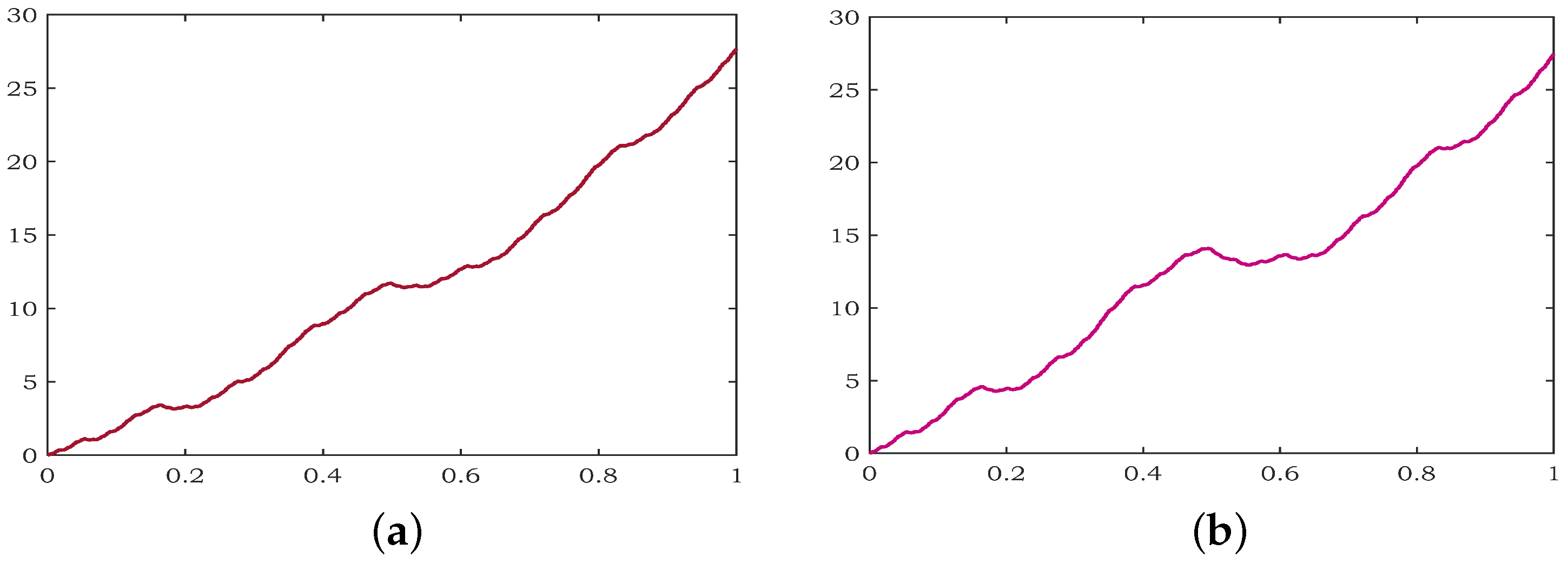
Observe the data points in Example 1 with the same scale vectors. Figure 2a presents theRL variable order fractional integral of f 1 with order μ ( s ) = 0.5 . Similarly, the graphical representation of theRL variable order fractional integral of f 2 with order μ ( s ) = 0.5 is displayed in Figure 2b. In both Figure 2a,b, the fractional order μ ( s ) is chosen to be the same μ ( s ) = 0.5 for clear comparison.
The following theorem explains the RL variable order fractional derivative of HVFIF with the preset initial condition ( D x 0 μ ( s ) f ) ( x 0 ) = 0 . The RL fractional derivative of variable order μ ( s ) where μ : [ a , b ] ( 0 , 1 ) , for a continuous function f is defined by the equation
D a μ ( s ) f ( x ) = 1 1 Γ ( μ ( s ) ) d d x a x f ( t ) ( x t ) μ ( s ) d t .
Suppose f is an HVFIF decisived by IFS (4); then, the RL fractional derivative of f of order μ ( s ) is defined as follows:
D a μ ( s ) f 1 ( x ) = 1 1 Γ ( μ ( s ) ) d d x a x f 1 ( t ) ( x t ) μ ( s ) d t ,
D a μ ( s ) f 2 ( x ) = 1 1 Γ ( μ ( s ) ) d d x a x f 2 ( t ) ( x t ) μ ( s ) d t .
Theorem 2.
Let f be the HVFIF given in Equations (2) and (3). If A k < 1 where A k = a k 1 μ ( s ) α k β k 0 γ k , for all k = 1 , 2 , , N , then ( D x 0 μ ( s ) f ) ( x ) = ( D x 0 μ ( s ) f 1 ) ( x ) , ( D x 0 μ ( s ) f 2 ) ( x ) is also an HVFIF. Further, ( D x 0 μ ( s ) f 1 ) ( x ) and ( D x 0 μ ( s ) f 2 ) ( x ) are determined by the IFSs L k ( x ) , F ^ 1 ( k , μ ( s ) ) ( x , y ^ , z ^ ) k = 1 N and L k ( x ) , F ^ 2 ( k , μ ( s ) ) ( x , z ^ ) k = 1 N , respectively, where F ^ 1 ( k , μ ( s ) ) ( x , y ^ , z ^ ) = a k 1 μ ( s ) α k y + a k 1 μ ( s ) β k z + p ^ k ( x ) and F ^ 2 ( k , μ ( s ) ) = a k 1 μ ( s ) γ k z + q ^ k ( x ) with k = 1 N a k 1 μ ( s ) α k 1 , k = 1 N a k 1 μ ( s ) γ k 1 , for k = 1 , 2 , , N .
Proof. 
The RL fractional derivative of f 1 is given by,
D x 0 μ ( s ) f 1 ( L k ( x ) ) = 1 1 Γ ( μ ( s ) ) d d x x 0 x k 1 f 1 ( t ) ( L k ( x ) t ) μ ( s ) d t + 1 1 Γ ( μ ( s ) ) d d x x 0 x k 1 f 1 ( t ) ( x k 1 t ) μ ( s ) f 1 ( t ) ( x k 1 t ) μ ( s ) d t + 1 1 Γ ( μ ( s ) ) d d x x k 1 L k ( x ) f 1 ( t ) ( L k ( x ) t ) μ ( s ) d u .
Replace the variable t = L k ( u ) in third term,
D x 0 μ ( s ) f 1 ( L k ( x ) ) = y ^ k 1 + f 1 ( k , μ ( s ) ) ( x ) + a k 1 Γ ( μ ( s ) ) d d x x 0 x f 1 ( L k ( u ) ) ( L k ( x ) L k ( u ) ) μ ( s ) d u .
Using the functional equation in Equation (7), we obtained the following equation:
( D x 0 μ ( s ) f 1 ) ( L k ( x ) ) = y ^ k 1 + f 1 ( k , μ ( s ) ) ( x ) + a k 1 Γ ( μ ( s ) ) d d x x 0 x ( α k f 1 ( u ) + β k f 2 ( u ) + p k ( x ) ) a k μ ( s ) ( x u ) μ ( s ) = y ^ k 1 + f 1 ( k , μ ( s ) ) ( x ) + a k 1 μ ( s ) α k ( D x 0 μ ( s ) f 1 ) ( x ) + a k 1 μ ( s ) β k ( D x 0 μ ( s ) f 2 ) ( x ) + a k 1 μ ( s ) ( D x 0 μ ( s ) p k ) ( x ) = a k 1 μ ( s ) α k ( D x 0 μ ( s ) f 1 ) ( x ) + a k 1 μ ( s ) β k ( D x 0 μ ( s ) f 2 ) ( x ) + p ^ k ( x ) .
Here, take p ^ k ( x ) = y ^ k 1 + f 1 ( k , μ ( s ) ) ( x ) + a k 1 μ ( s ) ( D x 0 μ ( s ) p k ) ( x ) , y ^ k 1 = 1 1 Γ ( μ ( s ) ) d d x x 0 x k 1 f 1 ( t ) ( x k 1 t ) μ ( s ) d t and f 1 ( k , μ ( s ) ) ( x ) = 1 1 Γ ( μ ( s ) ) d d x x 0 x k 1 ( f 1 ( t ) ( L k ( x ) t ) μ ( s ) f 1 ( t ) ( x k 1 t ) μ ( s ) ) d t . Now, consider the RL fractional derivative of f 2 of order μ ( s )
D x 0 μ ( s ) f 2 ( L k ( x ) ) = 1 1 Γ ( μ ( s ) ) d d x x 0 x k 1 f 2 ( t ) ( L k ( x ) t ) μ ( s ) d t + 1 1 Γ ( μ ( s ) ) d d x x 0 x k 1 f 2 ( t ) ( x k 1 t ) μ ( s ) f 2 ( t ) ( x k 1 t ) μ ( s ) d t + 1 1 Γ ( μ ( s ) ) d d x x k 1 L k ( x ) f 2 ( t ) ( L k ( x ) t ) μ ( s ) d t .
In the third term, replace t = L k ( u )
D x 0 μ ( s ) f 1 ( L k ( x ) ) = y ^ k 1 + f 1 ( k , μ ( s ) ) ( x ) + a k 1 Γ ( μ ( s ) ) d d x x 0 x f 2 ( L k ( u ) ) ( L k ( x ) L k ( u ) ) μ ( s ) d u .
The following equation is obtained using the functional equation in Equation (8):
( D x 0 μ ( s ) f 2 ) ( L k ( x ) ) = z ^ k 1 + f 2 ( k , μ ( s ) ) ( x ) + a k 1 Γ ( μ ( s ) ) d d x x 0 x ( γ k f 2 ( u ) + q k ( x ) ) a k μ ( s ) ( x u ) μ ( s ) = z ^ k 1 + f 2 ( k , μ ( s ) ) ( x ) + a k 1 μ ( s ) γ k ( D x 0 μ ( s ) f 2 ) ( x ) + a k 1 μ ( s ) ( D x 0 μ ( s ) q k ) ( x ) = a k 1 μ ( s ) γ k ( D x 0 μ ( s ) f 2 ) ( x ) + q ^ k ( x ) .
Here, q ^ k ( x ) = z ^ k 1 + f 2 ( k , μ ( s ) ) ( x ) + a k 1 μ ( s ) ( D x 0 μ ( s ) q k ) ( x ) , z ^ k 1 = 1 1 Γ ( μ ( s ) ) d d x x 0 x k 1 f 2 ( t ) ( x k 1 t ) μ ( s ) d t and f 2 ( k , μ ( s ) ) ( x ) = 1 1 Γ ( μ ( s ) ) d d x x 0 x k 1 ( f 2 ( t ) ( L k ( x ) t ) μ ( s ) f 2 ( t ) ( x k 1 t ) μ ( s ) ) d t . Hence, the RL variable order fractional derivative of HVFIF is also HVFIF. Consider the following:
D x 0 μ ( s ) f 1 ( L k ( x ) ) = y ^ k 1 + f 1 ( k , μ ( s ) ) ( x ) + a k 1 μ ( s ) α k ( D x 0 μ ( s ) f 1 ) ( x ) + a k 1 μ ( s ) β k ( D x 0 μ ( s ) f 2 ) ( x ) + a k 1 μ ( s ) ( D x 0 μ ( s ) p k ) ( x ) .
Let x = x N and L k ( x ) = x k . Then, the above equation provides,
y ^ k y ^ k 1 = f 1 ( k , μ ( s ) ) ( x N ) + a k 1 μ ( s ) y ^ N + a k 1 μ ( s ) β k ( D x 0 μ ( s ) f 2 ) ( x N ) + a k 1 μ ( s ) ( D x 0 μ ( s ) p k ) ( x N ) .
We know y ^ k = y ^ 0 + n = 1 k y ^ n y ^ n 1 , the aforementioned equation is as follows:
y ^ k = n = 1 k ( f 1 ( n , μ ( s ) ) ( x N ) + a n 1 μ ( s ) α n ( D x 0 μ ( s ) f 1 ) ( x N ) + a n 1 μ ( s ) β n ( D x 0 μ ( s ) f 2 ) ( x N ) + a n 1 μ ( s ) ( D x 0 μ ( s ) p n ) ( x N ) ) .
In Equation (17), y ^ N is obtained by converting k to N ,
y ^ N = n = 1 N ( f 1 ( n , μ ( s ) ) ( x N ) + a n 1 μ ( s ) β n ( D x 0 μ ( s ) f 2 ) ( x N ) + a n 1 μ ( s ) ( D x 0 μ ( s ) p n ) ( x N ) ) / 1 n = 1 N a n 1 μ ( s ) α n .
Consider the following equation to determine the new data set { ( x k , z ^ k ) : K = 0 , 1 , , N }
D x 0 μ ( s ) f 2 ( L k ( x ) ) = z ^ k 1 + f 2 ( k , μ ( s ) ) ( x ) + a k 1 μ ( s ) γ k ( D x 0 μ ( s ) f 2 ) ( x ) + a k 1 μ ( s ) ( D x 0 μ ( s ) q k ) ( x ) .
Let x = x N and L k ( x ) = x k
z ^ k z ^ k 1 = f 2 ( k , μ ( s ) ) ( x N ) + a k 1 μ ( s ) γ k z ^ N + a k 1 μ ( s ) ( D x 0 μ ( s ) q k ) ( x N ) .
We know z ^ k = z ^ 0 + n = 1 k z ^ n z ^ n 1 ; the aforementioned equation is as follows:
z ^ k = n = 1 k f 2 ( n , μ ( s ) ) ( x N ) + a n 1 μ ( s ) γ n z ^ N + a n 1 μ ( s ) ( D x 0 μ ( s ) q n ) ( x N ) .
In the Equation (18), z ^ N is obtained by converting k to N
z ^ N = n = 1 N f 2 ( n , μ ( s ) ) ( x N ) + a n 1 μ ( s ) ( D x 0 μ ( s ) q n ) ( x N ) / 1 n = 1 N a n 1 μ ( s ) γ n .
Remark 2.
Theorem 2 describes theRL variable order fractional derivative of HVFIF with the predefined condition ( D x 0 μ ( s ) f 1 ) ( x 0 ) = ( D x 0 μ ( s ) f 2 ) ( x 0 ) = 0 . Additionally, theRL variable order fractional derivative f is defined with the upper limit x N as
D x N μ ( s ) f 1 ( L k ( x ) ) = 1 1 Γ ( μ ( s ) ) d d x x x N f 1 ( t ) ( L k ( x ) t ) μ ( s ) d t
D x N μ ( s ) f 2 ( L k ( x ) ) = 1 1 Γ ( μ ( s ) ) d d x x x N f 2 ( t ) ( L k ( x ) t ) μ ( s ) d t
then one can obtain that function ( D x N μ ( s ) f ( L k ( x ) ) ) is again HVFIF with the variable order generated by the IFS { L k ( x ) , F ^ 1 ( k , μ ( s ) ) ( x , y ^ , z ^ ) } i = 1 N and { L k ( x ) , F ^ 2 ( k , μ ( s ) ) ( x , z ^ ) } i = 1 N where f 1 ^ ( x ) = y ^ k f 1 ( k , μ ( s ) ) ( x ) + a k 1 μ ( s ) α k ( D x N μ ( s ) f 1 ) ( x ) + a k 1 μ ( s ) β k ( D x N μ ( s ) f 2 ) ( x ) + a k 1 μ ( s ) ( D x N μ ( s ) p k ) ( x ) and f 2 ^ ( x ) = z ^ k f 2 ( k , μ ( s ) ) ( x ) + a k 1 μ ( s ) γ k ( D x N μ ( s ) f 2 ) ( x ) + a k 1 μ ( s ) ( D x N μ ( s ) q k ) ( x )
p ^ k ( x ) = y ^ k f 1 ( k , μ ( s ) ) ( x ) + a k 1 μ ( s ) ( D x N μ ( s ) p k ) ( x ) , y ^ k 1 = n = 1 k ( f 1 ( n , μ ( s ) ) ( x 0 ) a n 1 μ ( s ) α n y ^ 0 a n 1 μ ( s ) β n ( D x N μ ( s ) f 2 ) ( x 0 ) a n 1 μ ( s ) ( D x N μ ( s ) p n ) ( x 0 ) ) , y ^ 0 = n = 1 N ( f 1 ( n , μ ( s ) ) ( x 0 ) a n 1 μ ( s ) β n ( D x N μ ( s ) f 2 ) ( x 0 ) a n 1 μ ( s ) ( D x N μ ( s ) p n ) ( x 0 ) ) / 1 n = 1 N a n 1 μ ( s ) α n , q ^ k ( x ) = z ^ k f 2 ( k , μ ( s ) ) ( x ) + a k 1 μ ( s ) ( D x N μ ( s ) q k ) ( x ) , z ^ k 1 = n = 1 k f 2 ( n , μ ( s ) ) ( x 0 ) a n 1 μ ( s ) γ n z ^ 0 a n 1 μ ( s ) ( D x N μ ( s ) q n ) ( x 0 ) , z ^ 0 = n = 1 N f 2 ( n , μ ( s ) ) ( x 0 ) a n 1 μ ( s ) ( D x N μ ( s ) q n ) ( x 0 ) / 1 n = 1 N a n 1 μ ( s ) γ n .
If the variable order μ ( s ) is considered as a constant function, the above conclusion gives the Srijanani’s result [14]. The RL variable order fractional derivative of HVFIF with the predefined condition ( D x N μ ( s ) f ) ( x N ) = 0 is stated by the above remark.
Example 3.
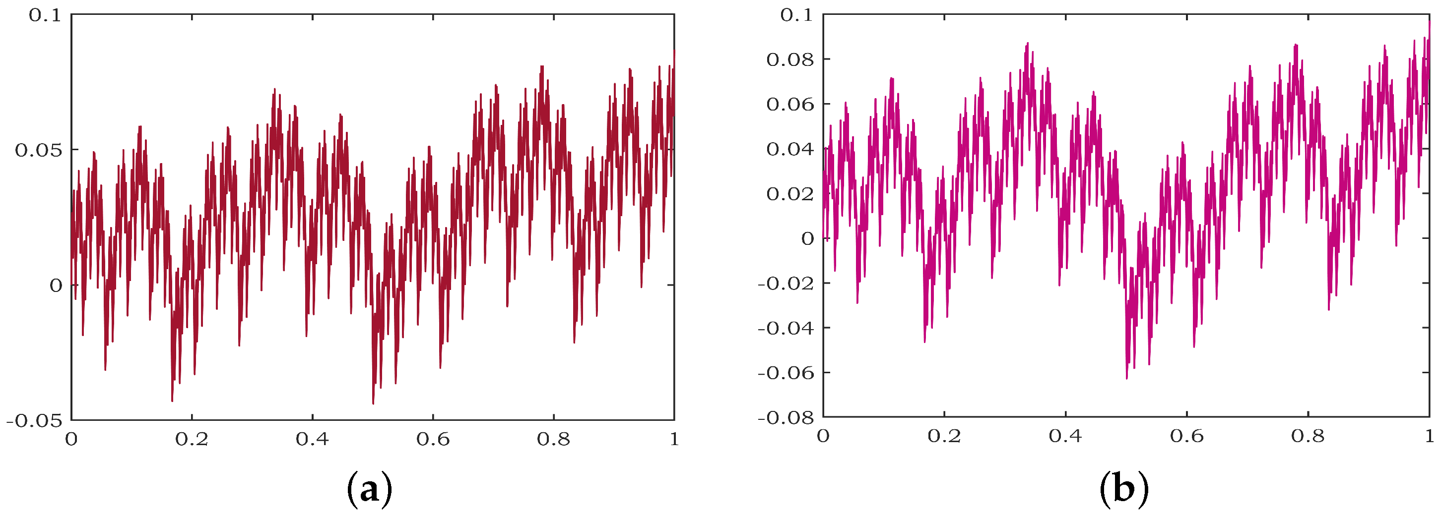
Consider the same data points and scale factors in Example 1 to obtain theRL variable order fractional derivative of f 1 and theRL variable order fractional derivative of f 2 . Figure 3a shows that D 0.5 f 1 and Figure 3b depict graphical representations of D 0.5 f 2 . The same choice of the fractional order μ ( s ) helps to observe the non-self affine and self-affine nature of D μ ( s ) f 1 and D μ ( s ) f 2 in Figure 3a,b respectively.
The WM variable order fractional derivative of HVFIF with a predetermined initial condition ( D x 0 μ ( s ) f ) ( x 0 ) = 0 is demonstrated in the following theorem.
Let variable order μ ( s ) , where μ : [ a , b ] ( 0 , 1 ) of the WM fractional derivative of continuous function f, be defined by the equation
( D x 0 μ ( s ) f ) ( x ) = μ ( s ) Γ ( 1 μ ( s ) ) a x f ( x ) f ( x t ) t 1 + μ ( s ) d t .
Suppose f is an HVFIF decisived by the IFS (4); then, the WM fractional derivative of f of order μ ( s ) is defined as follows:
( D x 0 μ ( s ) f 1 ) ( x ) = μ ( s ) Γ ( 1 μ ( s ) ) a x f 1 ( x ) f 1 ( x t ) t 1 + μ ( s ) d t ,
( D x 0 μ ( s ) f 2 ) ( x ) = μ ( s ) Γ ( 1 μ ( s ) ) a x f 2 ( x ) f 2 ( x t ) t 1 + μ ( s ) d t .
Theorem 3.
Let f be the HVFIF given in Equations (2) and (3). If A k < 1 where A k = a k μ ( s ) α k β k 0 γ k , for all k = 1 , 2 , , N , then ( D x 0 μ ( s ) f ) ( x ) = ( D x 0 μ ( s ) f 1 ) ( x ) , ( D x 0 μ ( s ) f 2 ) ( x ) is also an HVFIF. Further, ( D x 0 μ ( s ) f 1 ) ( x ) and ( D x 0 μ ( s ) f 2 ) ( x ) are determined by the IFSs L k ( x ) , F ^ 1 ( k , μ ( s ) ) ( x , y ^ , z ^ ) k = 1 N and L k ( x ) , F ^ 2 ( k , μ ( s ) ) ( x , z ^ ) k = 1 N , respectively, where F ^ 1 ( k , μ ( s ) ) ( x , y ^ , z ^ ) = a k μ ( s ) α k y + a k μ ( s ) β k z + p ^ k ( x ) and F ^ 2 ( k , μ ( s ) ) = a k μ ( s ) γ k z + q ^ k ( x ) with k = 1 N a k μ ( s ) α k 1 , k = 1 N a k μ ( s ) γ k 1 , for k = 1 , 2 , , N .
Proof. 
The WM fractional derivative Equation (20) gives,
( D x 0 μ ( s ) f 1 ) ( L k ( x ) ) = μ ( s ) Γ ( 1 μ ( s ) ) x 0 x k 1 f 1 ( x k 1 ) f 1 ( t ) ( x k 1 t ) 1 + μ ( s ) d t + μ ( s ) Γ ( 1 μ ( s ) ) x 0 x k 1 f 1 ( L k ( x ) ) f 1 ( t ) ( L k ( x ) t ) 1 + μ ( s ) f 1 ( x k 1 ) f 1 ( t ) ( x k 1 t ) 1 + μ ( s ) d t + μ ( s ) Γ ( 1 μ ( s ) ) x k 1 L k ( x ) f 1 ( L k ( x ) ) f 1 ( t ) ( L k ( x ) t ) 1 + μ ( s ) d t .
Replace t = L k ( u ) in the third term,
( D x 0 μ ( s ) f 1 ) ( L k ( x ) ) = y ^ k 1 + f 1 ( k , μ ( s ) ) ( x ) + a k μ ( s ) Γ ( 1 μ ( s ) ) x 0 x f 1 ( L k ( x ) ) f 1 ( L k ( u ) ) ( L k ( x ) L k ( u ) ) 1 + μ ( s ) d u .
The following equation is obtained using the functional equation Equation (7):
( D x 0 μ ( s ) f 1 ) ( L k ( x ) ) = y ^ k 1 + f 1 ( k , μ ( s ) ) ( x ) + a k μ ( s ) μ ( s ) α k Γ ( 1 μ ( s ) ) x 0 x f 1 ( x ) f 1 ( u ) ( x u ) 1 + μ ( s ) d u + a k μ ( s ) μ ( s ) β k Γ ( 1 μ ( s ) ) x 0 x f 2 ( x ) f 2 ( u ) ( x u ) 1 + μ ( s ) d u + a k μ ( s ) μ ( s ) Γ ( 1 μ ( s ) ) x 0 x p k ( x ) p k ( u ) ( x u ) 1 + μ ( s ) d u = y ^ n 1 + f 1 ( k , μ ( s ) ) ( x ) + a k μ ( s ) α k ( D x 0 μ ( s ) f 1 ) ( x ) + a k μ ( s ) β k ( D x 0 μ ( s ) f 2 ) ( x ) + a k μ ( s ) ( D x 0 μ ( s ) p k ) ( x ) = a k μ ( s ) α k ( D x 0 μ ( s ) f 1 ) ( x ) + a k μ ( s ) β k ( D x 0 μ ( s ) f 2 ) ( x ) + p ^ k , μ ( s ) ( x ) .
Here, p ^ k , μ ( s ) ( x ) = y ^ k 1 + f 1 ( k , μ ( s ) ) ( x ) + a k μ ( s ) ( D x 0 μ ( s ) p k ) ( x ) , y ^ k 1 = μ ( s ) Γ ( 1 μ ( s ) ) x 0 x k 1 f 1 ( x k 1 ) f 1 ( t ) ( x k 1 t ) 1 + μ ( s ) d t and f 1 ( k , μ ( s ) ) ( x ) = μ ( s ) Γ ( 1 μ ( s ) ) x 0 x k 1 f 1 ( L k ( x ) ) f 1 ( t ) ( L k ( x ) t ) 1 + μ ( s ) f 1 ( x k 1 ) f 1 ( t ) ( x k 1 t ) 1 + μ ( s ) d t . Now, consider the WM fractional derivative of f 2 of order μ ( s ) ,
( D x 0 μ ( s ) f 2 ) ( L k ( x ) ) = μ ( s ) Γ ( 1 μ ( s ) ) x 0 x k 1 f 2 ( x k 1 ) f 2 ( t ) ( x k 1 t ) 1 + μ ( s ) d t + μ ( s ) Γ ( 1 μ ( s ) ) x 0 x k 1 f 2 ( L k ( x ) ) f 2 ( t ) ( L k ( x ) t ) 1 + μ ( s ) f 2 ( x k 1 ) f 2 ( t ) ( x k 1 t ) 1 + μ ( s ) d t + μ ( s ) Γ ( 1 μ ( s ) ) x k 1 L k ( x ) f 2 ( L k ( x ) ) f 2 ( t ) ( L k ( x ) t ) 1 + μ ( s ) d t .
Replace t = L k ( u ) in the third term,
( D x 0 μ ( s ) f 2 ) ( L k ( x ) ) = y ^ k 1 + f 2 ( k , μ ( s ) ) ( x ) + a k μ ( s ) Γ ( 1 μ ( s ) ) x 0 x f 2 ( L k ( x ) ) f 2 ( L k ( u ) ) ( L k ( x ) L k ( u ) ) 1 + μ ( s ) d u .
The following equation is obtained using the functional equation Equation (8):
( D x 0 μ ( s ) f 2 ) ( L k ( x ) ) = z ^ k 1 + f 1 ( k , μ ( s ) ) ( x ) + a k μ ( s ) μ ( s ) γ k Γ ( 1 μ ( s ) ) x 0 x f 2 ( x ) f 2 ( u ) ( x u ) 1 + μ ( s ) d u + a k μ ( s ) μ ( s ) Γ ( 1 μ ( s ) ) x 0 x q k ( x ) q k ( u ) ( x u ) 1 + μ ( s ) d u = z ^ k 1 + f 2 ( k , μ ( s ) ) ( x ) + a k μ ( s ) γ k ( D x 0 μ ( s ) f 2 ) ( x ) + a k μ ( s ) ( D x 0 μ ( s ) q k ) ( x ) = a k μ ( s ) γ k ( D x 0 μ ( s ) f 2 ) ( x ) + q ^ k , μ ( s ) ( x ) .
Here, q ^ k , μ ( s ) ( x ) = z ^ k 1 + f 2 ( k , μ ( s ) ) ( x ) + a k μ ( s ) ( D x 0 μ ( s ) q k ) ( x ) , z ^ k 1 = μ ( s ) Γ ( 1 μ ( s ) ) x 0 x k 1 f 2 ( x k 1 ) f 2 ( t ) ( x k 1 t ) 1 + μ ( s ) d t and f 1 ( k , μ ( s ) ) ( x ) = μ ( s ) Γ ( 1 μ ( s ) ) x 0 x k 1 f 1 ( L k ( x ) ) f 1 ( t ) ( L k ( x ) t ) 1 + μ ( s ) f 1 ( x k 1 ) f 1 ( t ) ( x k 1 t ) 1 + μ ( s ) d t . Hence, the WM variable order fractional derivative of HVFIF is also HVFIF. Consider the following equation for calculating new data points:
( D x 0 μ ( s ) f 1 ) ( L k ( x ) ) = y ^ k 1 + f 1 ( k , μ ( s ) ) ( x ) + a k μ ( s ) α k ( D x 0 μ ( s ) f 1 ) ( x ) + a k μ ( s ) β k ( D x 0 μ ( s ) f 2 ) ( x ) + a k μ ( s ) ( D x 0 μ ( s ) p k ) ( x ) .
Let x = x N and L k ( x N ) = x k . Then, the above equation gives
y ^ k y ^ k 1 = f 1 ( k , μ ( s ) ) ( x N ) + a k μ ( s ) α k y ^ N + a k μ ( s ) β k ( D x 0 μ ( s ) f 2 ) ( x N ) + a k μ ( s ) ( D x 0 μ ( s ) p k ) ( x ) .
The aforementioned equation is as follows when considered from the perspective of the equation y ^ k = y ^ 0 + n = 1 k ( y ^ n y ^ n 1 ) :
y ^ k = n = 1 k ( f 1 ( n , μ ( s ) ) ( x N ) + a n μ ( s ) α n y ^ N + a n μ ( s ) β n ( D x 0 μ ( s ) f 2 ) ( x N ) + a n μ ( s ) ( D x 0 μ ( s ) p n ) ( x N ) ) .
In Equation (22), y ^ N is obtained by varying k to N
y ^ N = n = 1 N ( f 1 ( n , μ ( s ) ) ( x N ) + a n μ ( s ) β n ( D x 0 μ ( s ) f 2 ) ( x N ) + a n μ ( s ) ( D x 0 μ ( s ) p n ) ( x N ) ) / 1 n = 1 N a n μ ( s ) d n .
Consider the following equation to determine the new data set { ( x k , z ^ k ) : K = 0 , 1 , , N }
D x 0 μ ( s ) f 2 ( L k ( x ) ) = z ^ k 1 + f 2 ( k , μ ( s ) ) ( x ) + a k μ ( s ) γ k ( D x 0 μ ( s ) f 2 ) ( x ) + a k μ ( s ) ( D x 0 μ ( s ) q k ) ( x ) .
Let x = x N and L k ( x ) = x k . Then, the above equation yields,
z ^ k z ^ k 1 = f 2 ( k , μ ( s ) ) ( x N ) + a k μ ( s ) γ k z ^ N + a k μ ( s ) ( D x 0 μ ( s ) q k ) ( x N ) .
The aforementioned equation is as follows when considered from the perspective of the equation z ^ k = z ^ 0 + n = 1 k z ^ n z ^ n 1 :
z ^ k = n = 1 k f 2 ( n , μ ( s ) ) ( x N ) + a n μ ( s ) γ n z ^ N + a n μ ( s ) ( D x 0 μ ( s ) q n ) ( x N ) .
In Equation (23), z ^ N is obtained by varying k to N
z ^ N = n = 1 N f 2 ( n , μ ( s ) ) ( x N ) + a n μ ( s ) ( D x 0 μ ( s ) q n ) ( x N ) / 1 n = 1 N a n μ ( s ) γ n .
Remark 3.
TheWM fractional derivative with the variable order of HVFIF is demonstrated in Theorem 3 with a predefined condition ( D x 0 μ ( s ) f 1 ) ( x 0 ) = ( D x 0 μ ( s ) f 2 ) ( x 0 ) = 0 . Similarly, theWM variable order fractional derivative f is defined with the upper limit x N as
( D x N μ ( s ) f 1 ) ( L k ( x ) ) = μ ( s ) Γ ( 1 μ ( s ) ) x x N f 1 ( L k ( x ) ) f 1 ( t ) ( L k ( x ) t ) 1 + μ ( s ) d t
( D x N μ ( s ) f 2 ) ( L k ( x ) ) = μ ( s ) Γ ( 1 μ ( s ) ) x x N f 2 ( L k ( x ) ) f 2 ( t ) ( L k ( x ) t ) 1 + μ ( s ) d t
then, one can obtain that function ( D x N μ ( s ) f ( L k ( x ) ) is again HVFIF with the variable order generated by the IFS { L k ( x ) , F ^ 1 ( k , μ ( s ) ) ( x , y ^ , z ^ ) } i = 1 N and { L k ( x ) , F ^ 2 ( k , μ ( s ) ) ( x , z ^ ) } i = 1 N where f 1 ^ ( x ) = y ^ k f 1 ( k , μ ( s ) ) ( x ) + a k μ ( s ) α k ( D x N μ ( s ) f 1 ) ( x ) + a k μ ( s ) β k ( D x N μ ( s ) f 2 ) ( x ) + a k μ ( s ) ( D x N μ ( s ) p k ) ( x ) and f 2 ^ ( x ) = z ^ k f 2 ( k , μ ( s ) ) ( x ) + a k μ ( s ) γ k ( D x N μ ( s ) f 2 ) ( x ) + a k μ ( s ) ( D x N μ ( s ) q k ) ( x )
p ^ k ( x ) = y ^ k f 1 ( k , μ ( s ) ) ( x ) + a k μ ( s ) ( D x N μ ( s ) p k ) ( x ) , y ^ k 1 = n = 1 k ( f 1 ( n , μ ( s ) ) ( x 0 ) a n μ ( s ) α n y ^ 0 a n μ ( s ) β n ( D x N μ ( s ) f 2 ) ( x 0 ) a n μ ( s ) ( D x N μ ( s ) p n ) ( x 0 ) ) , y ^ 0 = n = 1 N ( f 1 ( n , μ ( s ) ) ( x 0 ) a n μ ( s ) β n ( D x N μ ( s ) f 2 ) ( x 0 ) a n μ ( s ) ( D x N μ ( s ) p n ) ( x 0 ) ) / 1 n = 1 N a n μ ( s ) α n , q ^ k ( x ) = z ^ k f 2 ( k , μ ( s ) ) ( x ) + a k μ ( s ) ( D x N μ ( s ) q k ) ( x ) , z ^ k 1 = n = 1 k f 2 ( n , μ ( s ) ) ( x 0 ) a n μ ( s ) γ n z ^ 0 a n μ ( s ) ( D x N μ ( s ) q n ) ( x 0 ) , z ^ 0 = n = 1 N f 2 ( n , μ ( s ) ) ( x 0 ) a n μ ( s ) ( D x N μ ( s ) q n ) ( x 0 ) / 1 n = 1 N a n μ ( s ) γ n .
When the variable order μ ( s ) is considered as a constant function, the above conclusion provides Priyanka’s [27] result.
Example 4.
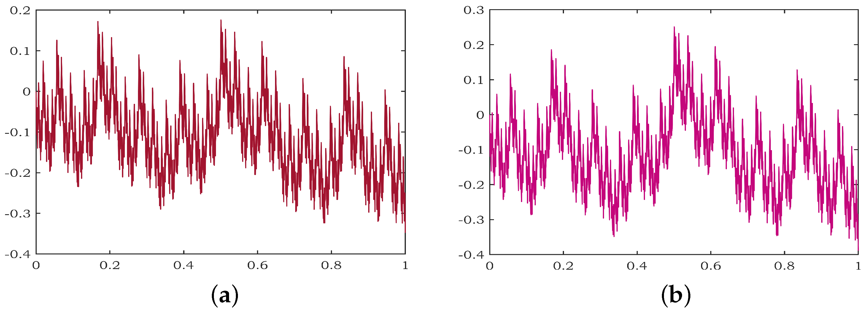
TheWM variable order fractional derivative of f 1 and theWM variable order fractional derivative of f 2 are calculated using the same data points and scale factors as in Example 1. D 0.5 f 1 is shown in Figure 4a, while a graphical representation of D 0.5 f 2 is given in Figure 4b.

4. Concluding Remarks

This work introduces a novel approach to investigate variable order fractional integration. The evaluation of fractional integration and differentiation with continuously varying-order μ ( s ) for each s [ x 0 , x N ] is associated with the change of constant fractional order μ as a function of s. The RL variable order fractional calculus and the WM variable order fractional derivative of the HVFIF are explored with predefined initial conditions. Further, the resultant functions are demonstrated as the HVFIF.

Author Contributions

Methodology, V.R.; Formal analysis, A.G.; Writing—review & editing, V.R. All of the authors contributed equally in this research work. All authors have read and agreed to the published version of the manuscript.

Funding

The authors acknowledge the financial support by the VIT.

Data Availability Statement

Not applicable.

Conflicts of Interest

The authors declare no conflict of interest.

References

  1. Barnsley, M.F. Fractal functions and interpolation. Constr. Approx. 1986, 2, 303–329. [Google Scholar] [CrossRef]
  2. Hutchinson, J.E. Fractals and self similarity. Indiana Univ. Math. J. 1981, 30, 713–747. [Google Scholar] [CrossRef]
  3. Easwaramoorthy, D.; Uthayakumar, R. Analysis on fractals in fuzzy metric spaces. Fractals 2011, 19, 379–386. [Google Scholar] [CrossRef]
  4. Banerjee, S.; Easwaramoorthy, D.; Gowrisankar, A. Fractal Functions, Dimensions and Signal Analysis; Springer: Cham, Switzerland, 2021. [Google Scholar]
  5. Banerjee, S.; Hassan, M.K.; Mukherjee, S.; Gowrisankar, A. Fractal Patterns in Nonlinear Dynamics and Applications; CRC Press: Boca Raton, FL, USA, 2020. [Google Scholar]
  6. Ruan, H.J.; Su, W.Y.; Yao, K. Box dimension and fractional integral of linear fractal-interpolation functions. J. Approx. Theory 2009, 161, 187–197. [Google Scholar] [CrossRef] [Green Version]
  7. Balasubramani, N. Affine recurrent fractal-interpolation functions. Eur. Phys. J. Spec. Top. 2021, 230, 3765–3779. [Google Scholar] [CrossRef]
  8. Barnsley, M.F.; Elton, J.; Hardin, D.; Massopust, P. Hidden variable fractal interpolation functions. Siam J. Math. Anal. 1989, 20, 1218–1242. [Google Scholar] [CrossRef]
  9. Chand, A.K.B.; Kapoor, G.P. Hidden variable bivariate fractal interpolation surfaces. Fractals 2003, 11, 277–288. [Google Scholar] [CrossRef]
  10. Bouboulis, P.; Dalla, L. Hidden variable vector valued fractal-interpolation functions. Fractals-London 2003, 13, 227. [Google Scholar] [CrossRef]
  11. Bouboulis, P.; Dalla, L.; Drakopoulos, V. Construction of recurrent bivariate fractal interpolation surfaces and computation of their box-counting dimension. J. Approx. Theory 2006, 141, 99–117. [Google Scholar] [CrossRef] [Green Version]
  12. Chand, A.K.B.; Kapoor, G.P. Cubic spline coalescence fractal interpolation through moments. Fractals 2007, 15, 41–53. [Google Scholar] [CrossRef]
  13. Kapoor, G.P.; Prasad, S.A. Smoothness of hidden variable bivariate coalescence fractal interpolation surfaces. Int. J. Bifurcat. Chaos 2009, 19, 2321–2333. [Google Scholar] [CrossRef] [Green Version]
  14. Prasad, S.A. Fractional calculus of coalescence hidden variable fractal interpolation functions. Fractals 2009, 25, 1750019. [Google Scholar] [CrossRef]
  15. Priyanka, T.M.C.; Gowrisankar, A. Analysis on Weyl–Marchaud Fractional Derivative for Types of fractal-interpolation function with Fractal Dimension. Fractals 2021, 29, 2150215. [Google Scholar] [CrossRef]
  16. Ri, M.G.; Yun, C.H.; Kim, M.H. Construction of cubic spline hidden variable recurrent fractal-interpolation function and its fractional calculus. Chaos Solitons Fractals 2021, 150, 111177. [Google Scholar] [CrossRef]
  17. Ri, M.G.; Yun, C.H. Smoothness and fractional integral of hidden variable recurrent fractal-interpolation function with function vertical scaling factors. Fractals 2021, 29, 2150136. [Google Scholar] [CrossRef]
  18. Gowrisankar, A.; Uthayakumar, R. Fractional calculus on fractal interpolation for a sequence of data with countable iterated function system. Mediterr. J. Math. 2016, 13, 3887–3906. [Google Scholar] [CrossRef]
  19. Gowrisankar, A.; Khalili Golmankhaneh, A.; Serpa, C. Fractal Calculus on fractal-interpolation functions. Fractal Fract. 2021, 5, 157. [Google Scholar] [CrossRef]
  20. Yao, K.; Su, W.Y.; Zhou, S.P. The fractional derivatives of a fractal function. Acta Math. Sin. 2006, 22, 719–722. [Google Scholar] [CrossRef]
  21. Ri, M.G.; Yun, C.H. Riemann–Liouville fractional integral of hidden variable fractal interpolation function. Chaos Solitons Fractals 2020, 140, 110126. [Google Scholar] [CrossRef]
  22. Liang, Y.S.; Su, W.Y. Fractal dimensions of fractional integral of continuous functions. Acta Math. Sin.-Engl. Ser. 2016, 32, 1494–1508. [Google Scholar] [CrossRef]
  23. Zhang, Q. Some remarks on one-dimensional functions and their Riemann–Liouville fractional calculus. Acta Math. Sin.-Engl. Ser. 2014, 30, 517–524. [Google Scholar] [CrossRef]
  24. Gowrisankar, A.; Prasad, M. Riemann–Liouville calculus on quadratic fractal-interpolation function with variable scaling factors. J. Anal. 2019, 27, 347–363. [Google Scholar] [CrossRef]
  25. Peng, W.L.; Yao, K.; Zhang, X.; Yao, J. Box dimension of Weyl–Marchaud fractional derivative of linear fractal-interpolation functions. Fractals 2019, 27, 1950058. [Google Scholar] [CrossRef]
  26. Ferrari, F. Weyl and Marchaud derivatives: A forgotten history. Mathematics 2018, 6, 6. [Google Scholar] [CrossRef] [Green Version]
  27. Priyanka, T.M.C.; Gowrisankar, A. Riemann–Liouville fractional integral of non-affine fractal-interpolation function and its fractional operator. Eur. Phys. J. Spec. Top. 2021, 230, 3789–3805. [Google Scholar] [CrossRef]
  28. Ri, M.G.; Yun, C.H. Riemann–Liouville fractional derivatives of hidden variable recurrent fractal-interpolation functions with function scaling factors and box dimension. Chaos Solitons Fractals 2022, 156, 111793. [Google Scholar] [CrossRef]
  29. Samko, S.G.; Ross, B. Integration and differentiation to a variable fractional order. Integr. Transform. Spec. Funct. 1993, 1, 277–300. [Google Scholar] [CrossRef]
  30. Samko, S.G. Fractional integration and differentiation of variable order. Anal. Math. 1995, 21, 213–236. [Google Scholar] [CrossRef]
  31. Zhao, X.; Sun, Z.Z.; Karniadakis, G.E. Second-order approximations for variable order fractional derivatives: Algorithms and applications. J. Comput. Phys. 2015, 293, 184–200. [Google Scholar] [CrossRef]
  32. Garrappa, R.; Giusti, A.; Mainardi, F. variable order fractional calculus: A change of perspective. Commun. Nonlinear Sci. Numer. Simul. 2021, 102, 105904. [Google Scholar] [CrossRef]
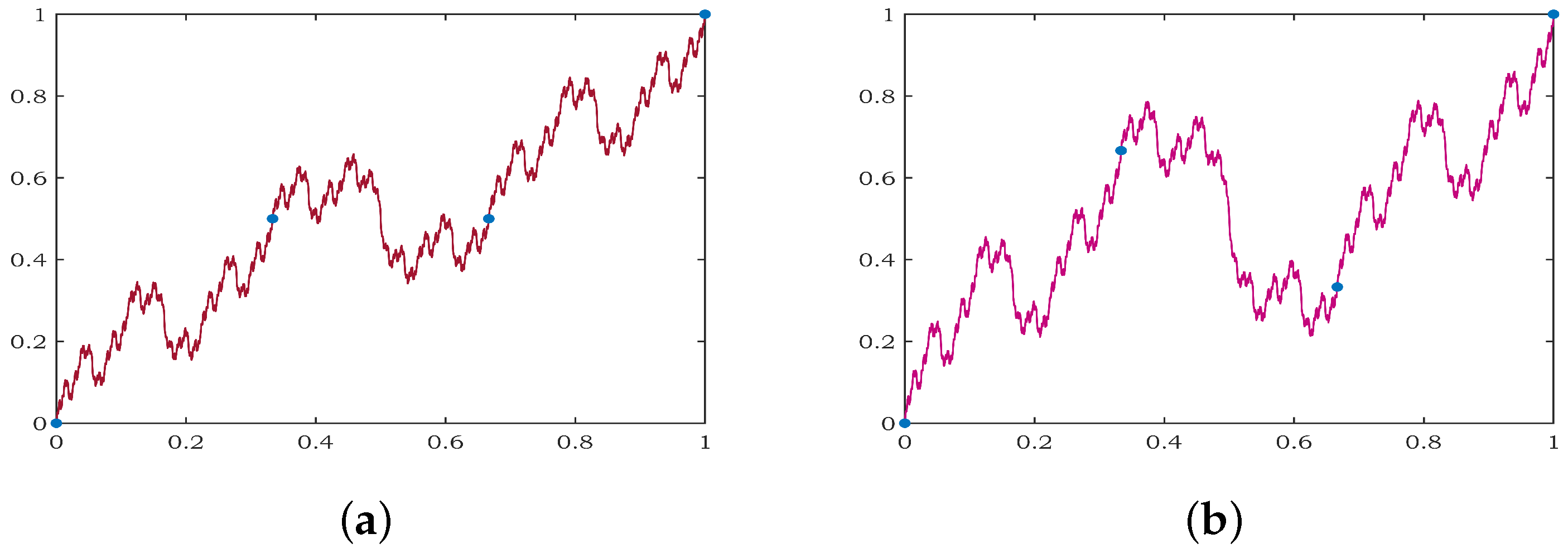
Figure 1. Hidden variable fractal interpolation function: (a) non-self-affine f 1 , (b) self-affine f 2 .
Fractalfract 07 00034 g001
Figure 2. The RL fractional integral: (a) I μ ( s ) f 1 with variable order μ ( s ) = 0.5 , (b) I μ ( s ) f 2 with order μ ( s ) = 0.5 .
Fractalfract 07 00034 g002
Figure 3. The RL fractional derivative: (a) D μ ( s ) f 1 with variable order μ ( s ) = 0.5 ; (b) D μ ( s ) f 2 with order μ ( s ) = 0.5 .
Fractalfract 07 00034 g003
Figure 4. The WM fractional derivative: (a) D μ ( s ) f 1 with variable order μ ( s ) = 0.5 , (b) D μ ( s ) f 2 with order μ ( s ) = 0.5 .
Fractalfract 07 00034 g004
Disclaimer/Publisher’s Note: The statements, opinions and data contained in all publications are solely those of the individual author(s) and contributor(s) and not of MDPI and/or the editor(s). MDPI and/or the editor(s) disclaim responsibility for any injury to people or property resulting from any ideas, methods, instructions or products referred to in the content.