


Characteristic Analysis and Circuit Implementation of a Novel Fractional-Order Memristor-Based Clamping Voltage Drift

1
Xi’an Key Laboratory of Human-Machine Integration and Control Technology for Intelligent Rehabilitation, School of Computer Science, Xijing University, Xi’an 710123, China
2
Shaanxi International Joint Research Center for Applied Technology of Controllable Neutron Source, School of Electronic Information, Xijing University, Xi’an 710123, China
3
Academy of Advanced Interdisciplinary Research, Xidian University, Xi’an 710071, China
*
Author to whom correspondence should be addressed.
Fractal Fract. 2023, 7(1), 2; https://doi.org/10.3390/fractalfract7010002
Submission received: 6 November 2022
/
Revised: 9 December 2022
/
Accepted: 12 December 2022
/
Published: 20 December 2022
(This article belongs to the Special Issue Recent Advances in Fractional-Order Neural Networks: Theory and Application)
Abstract
:The ideal magnetic flux-controlled memristor was introduced into a four-dimensional chaotic system and combined with fractional calculus theory, and a novel four-dimensional commensurate fractional-order system was proposed and solved using the Adomian decomposition method. The system orders, parameters, and initial values were studied as independent variables in the bifurcation diagram and Lyapunov exponents spectrum, and it was discovered that changing these variables can cause the system to exhibit more complex and rich dynamical behaviors. The system had an offset boosting, which was discovered by adding a constant term after the decoupled linear term. Finally, the results of the numerical simulation were verified through the use of analog circuits and FPGA designs, and a control scheme for the system circuit was also suggested.
1. Introduction
The first chaotic system was accidentally proposed by Lorenz [1], and scholars began to investigate various chaotic systems with different types of attractors [2,3,4,5,6,7] and equilibria [8,9,10,11]. The exceptional qualities of chaotic systems, such as their initial sensitivity and long-term unpredictability, allow for their cross-combination with other scientific disciplines, including image encryption [12], finance [13], and so forth. It has therefore become a priority to figure out how to establish new chaotic systems with improved physical properties, and the establishment of memristive chaotic system is an effective method [14]. Leon Chua once proposed the fourth fundamental element from a symmetry arguments memristor, which serves as the link between magnetic flux and charge [15]. In recent years, memristors have received much attention due to their unique non-volatile performance and variety of nonlinear characteristics, such as their Lissajous curve’s variation with frequency and the appearance of the voltage–current’s hysteresis curve shrinking at the origin [16]. By introducing memristors with different properties into the existing chaotic circuit systems, scholars have obtained a new class of memristive chaotic circuit systems, studied their abundantly rich dynamical behaviors [17,18,19,20,21], and used them to establish nonlinear circuits [22], neural networks [23,24], secure communications [25], and other engineering fields. However, most of these studies are based on the integer-order calculus system. Fractional-order calculus can accurately describe the physical model as a generalized description. Therefore, it has drawn the attention of scholars and has become the focus of nonlinear theory and engineering application studies.
The theoretical development of fractional-order calculus has been very slow due to a lack of practical engineering experience and the substantial amount of calculations using traditional pens. However, with the advancement of computer technology in recent years and the inclusion of variable differences in the range of , numerous fields increasingly focus on fractional-calculus operators. Meanwhile, the combination of fractional-order calculus and memristors expands the influence of control parameters on the system performance and exhibits richer dynamical behaviors, including high-dimensional [26] and variable-order memristive chaotic systems [27]. With an increased study depth, scholars have begun to shift their original focus from the dynamical behaviors of chaotic memristive circuits with different parameters [28,29,30] to the study of memristive chaotic systems with changing initial values [31,32]. As a result, we can investigate a novel fractional-order memristor chaotic system and, by altering the initial value, can make the system exhibit extreme multistability. This can improve the complexity of chaotic pseudo-random sequences and better satisfy the requirements of code division multiple access and the spread spectrum in secure communication [33,34,35].
Meanwhile, a number of non-ideal issues with memristor operation have emerged in recent years along with the development of memristors, including random variability, voltage-drift and the aging-induced degradation of the memristor threshold voltage [36,37]. When we designed the memristive chaotic circuit, the integrator was made by the operational amplifier, and the positive input was grounded. The integration function was obtained by using the virtual short concept of the two inputs of the ideal operational amplifier, where the negative terminal is also zero. However, the input of the operational amplifier exists as offset; that is, when the positive input terminal is grounded, the negative input terminal is not zero, the input offset is also integrated, and the output terminal has voltage. Thus, the DC voltage integration drift occurs. Consequently, the current study will concentrate on how to design memristive chaotic circuits to clamp voltage integration drift. The paper is organized as follows: In Section 2, the mathematical expression of a fractional memristor is derived through fractional calculus theory. The performance of the memristor is studied through numerical research and circuit implementation. In Section 3, when orders, system parameters, and system initial values are selected as variables, the bifurcation diagram and Lyapunov exponents (LEs) spectrum are used to illustrate the characteristics of the system and then the offset boosting phenomenon of the system is researched. In Section 4, the analog circuit and FPGA design of the multi-type chaotic attractor are implemented, and the control circuit of the system is designed through the stability analysis of the equilibrium to satisfy the control requirements. The last section summarizes the work of this paper and gives prospects for future work.
2. Fractional-Order Chaotic Memristor Circuit and Model
2.1. Fractional-Order Calculus
The operator is generally used to represent fractional-order calculus. D is a differential operator, d stands for the differential definition, and t are the boundaries of the operator, and q is a real number. When q is positive, it is a differentiation, and when q is negative, it is an integration. Different from integer-order calculus, there are many definitions of fractional-order calculus, among which, the Caputo definition [38] is more common, which is as follows:
where , , is a gamma function, and C is the Caputo differential definition. When , , the properties of Caputo fractional-order calculus are
is the q-order integral operator, is the q-order differential operator, and . When , . In practical application, the definition of the fractional-order derivative of time is often defined by Caputo. From [39], we can obtain ; then, according to Euler’s equation , we can expand it as follows:
Thus, Equation (3) can be
and, for Equation (4) above, the fractional-order derivative formulae of sine and cosine functions are obtained by expanding the corresponding real and imaginary parts of Euler’s Equation (3). Then, from the short-term memory principle [39], when , Equation (4) can be approximated as
the corresponding fractional-order integral is as follows:
Therefore, when , we can obtain
the subsequent derivation of the memristor model will make extensive use of many of the equations mentioned above that are related to this section.
2.2. Fractional-Order Memristor Model and Circuit
2.2.1. Magnetic Flux-Controlled Memristor Model
The model of the nonlinear fractional-order quadratic memristor is
where , is the input current, is the output voltage, is the memristor value, and are parameters, is the memristor internal variable, and . The driving voltage on both sides of the memristor is , and through Equations (7) and (8) simultaneously, we have
where is the amplitude and is the angular frequency. Then, from the short-term memory principle [39], Equation (9) can be approximated as
and by integrating the two sides of Equation (10), we obtain
When , the above expression is simplified to an integer-order memristor equation and, when , Equations (11) and (8) simultaneously become
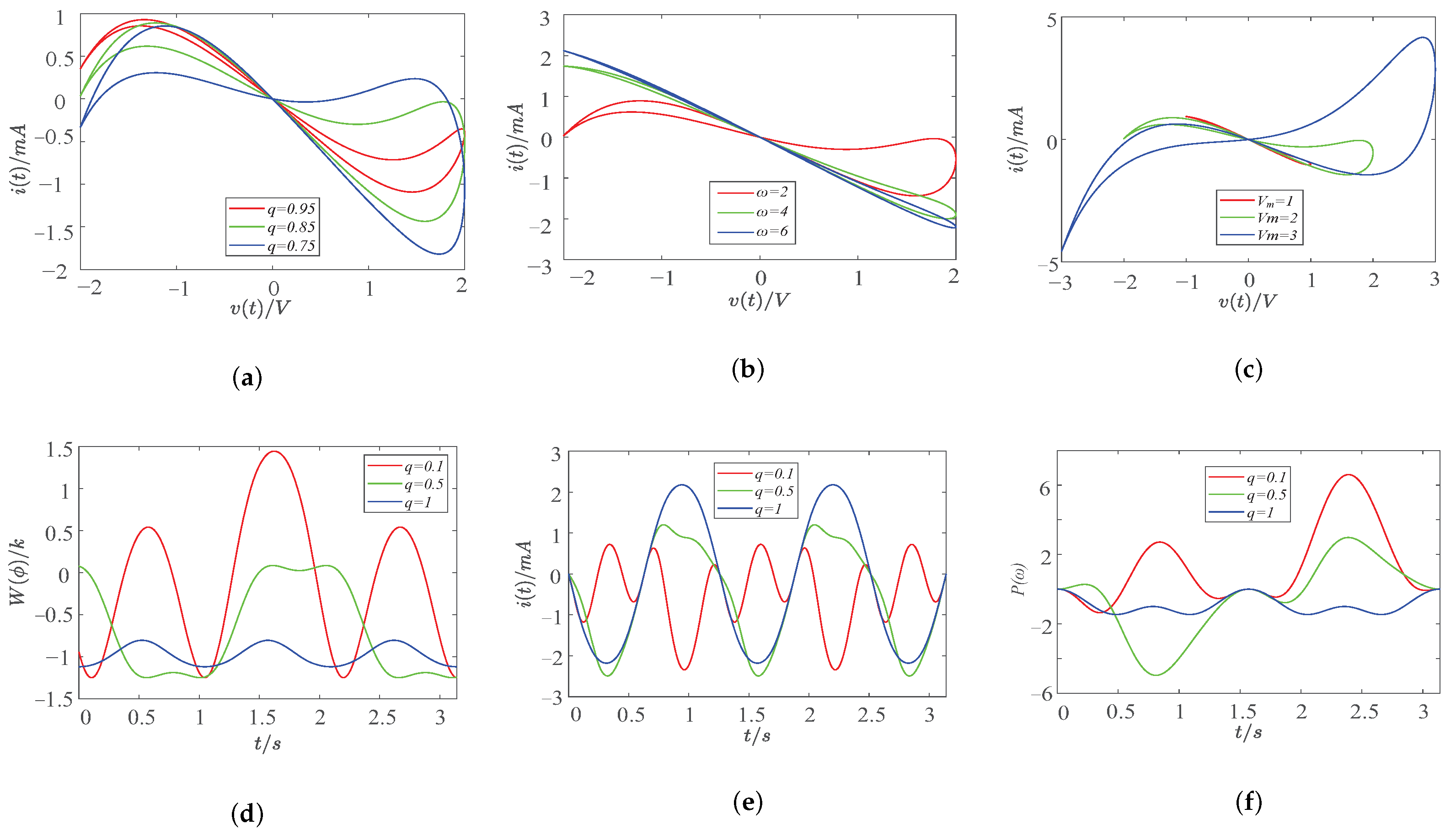
According to Equation (12), the system parameters of the memristor, the initial magnetic flux of the memristor, and the amplitude and frequency of the sinusoidal voltage excitation are all related to the current flowing through the quadratic nonlinear magnetic flux-controlled memristor. When the input voltage is , for different amplitudes and frequencies of sinusoidal voltage excitation and different internal initial conditions of the memristor, the quadratic nonlinear flux memristor hysteresis loop on the plane is shown in Figure 1a–c, and Figure 1d–f displays the memristor’s time-domain waveform.
From above, Figure 1a shows the alter of the area of the hysteresis loop when the order q of Equation (12) is changed; Figure 1b illustrates how the area of the hysteresis loop changes when the frequency is altered, and, when the increment is large enough, it becomes a single-valued function; Figure 1c shows that there is a positive correlation between the variation in the excitation voltage amplitude at the memristor terminal and the area of the hysteresis loop. Then, in the subsequent group, Figure 1d is the effect of order on the memristor, and the memristance will be positive or negative. When the fractional-order memristor degenerates to integer-order, it is found that the integer-order memristance is always negative; Figure 1e demonstrates that the dynamic range of the current memristor variation increases with a decreasing order; Figure 1f is the time-domain waveform of the memristor output power, and when the order changes, the memristor power changes between positive and negative. When the fractional-order memristor degenerates into an integer-order, the integer-order memristor power is always less than zero.
2.2.2. Implementation of Chaotic Circuit
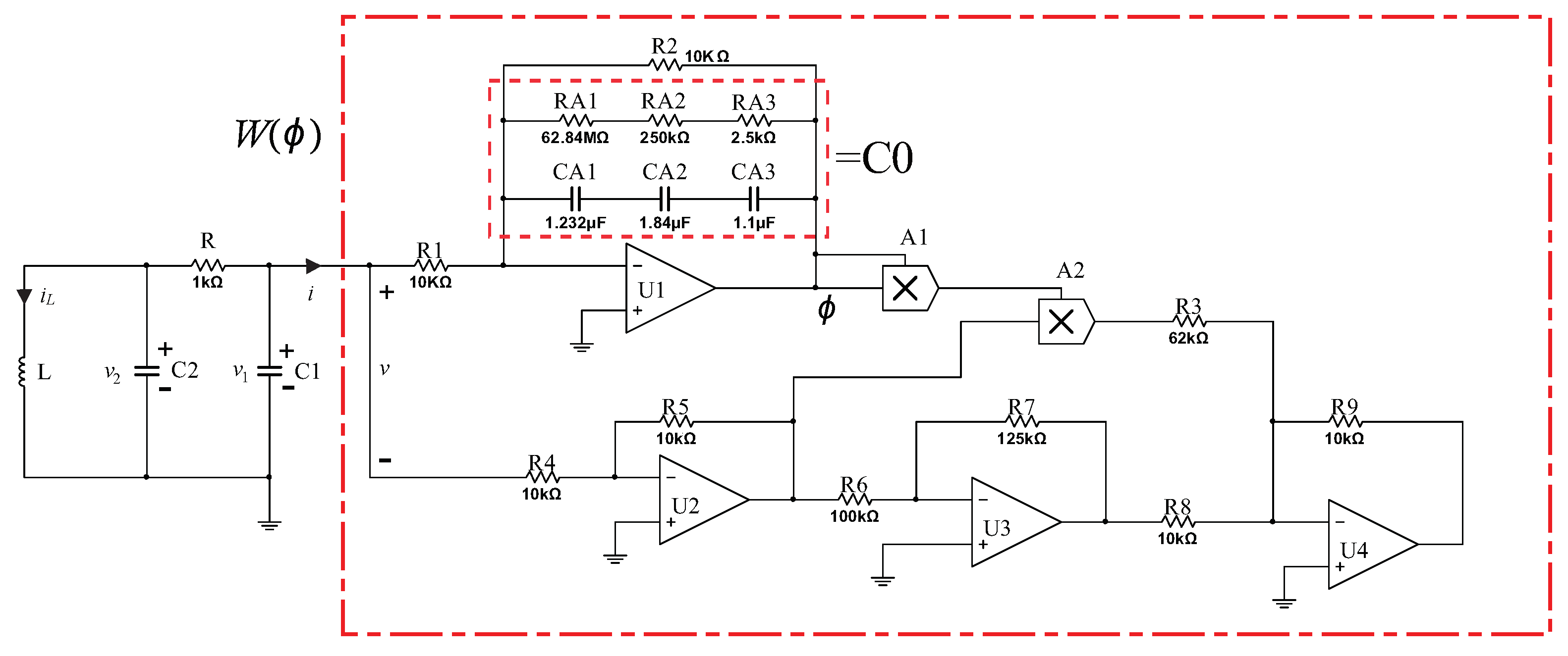
According to the nonlinear magnetic flux-controlled memristor model described in Equation (12), parameters were set and the equivalent circuit of the fractional-order memristor was established, as shown in Figure 2, where, different from the traditional active magnetic flux-controlled memristor, a shunt resistor was added to the integrating capacitor to clamp the DC voltage integral drift. Furthermore, the fractional-order memristor model is
where v and i represent the input voltage and current, respectively, and is the voltage at both ends of the integrating capacitor . The circuit unit values involved in the equation are shown in Table 1.
Following that, different excitation amplitudes and frequencies of a sinusoidal voltage source can be chosen in accordance with the parameters in Table 1 to simulate various hysteresis loops shrinking at the origin in Multism, as shown in Figure 3.
Figure 3a shows that the voltage excited by sinusoidal voltages has not changed, but the frequencies have changed: this is a “hard” switching condition (large voltage excursions or long-term bias), and any symmetrical AC voltage bias will cause double-loop hysteresis and shrink to a line at high frequency (blue line) as long as it remains in the memristor mechanism. Figure 3b shows that the frequencies have not changed and that the voltages have changed, and as the voltage decreases, the hysteresis loop of the memristor tends to be linear.
2.2.3. Dynamical Chaotic Circuit Model
According to Figure 2, the dynamical elements, capacitance and , inductance L, and magnetic flux-controlled memristor correspond to state variables , , , and , respectively. Therefore, the equations of state can be described by Kirchhoff voltage law as
where . Let , , , and . Define nonlinear function , and then let , , , , , , , , , and . The normalized representation of Equation (14) can be rewritten as
where q represents the fractional order of the commensurate system, and a, b, c, d, e, and f are the system parameters.
2.3. Adomian Decomposition Algorithm and Solution
2.3.1. Adomian Decomposition Algorithm
The Adomian decomposition algorithm is a numerical analysis algorithm with a high accuracy and fast convergence. Its general method is to decompose the differential equation into nonlinear terms, linear terms, and constant terms, convert the nonlinear terms into a special polynomial, and then use the inverse operator method to derive step by step. Finally, the approximate solution of the differential equation is obtained. It is the best candidate method for solving fractional-order chaotic systems at present. is the function variable, where , represents the Caputo differential operator of q-order, whereupon its expression, based on the Adomian decomposition algorithm, is as follows:
where, , and , the linear operator of the system can be represented by L and the nonlinear operator can be represented by N, the representative constant and the representative initial value. From Equation (2), fractional integration operator on both sides of Equation (16), and we get
where . From the properties of fractional integral operators [38], the nonlinear term in Equation (17) can be decomposed according to Equation (18):
where , . Then, the nonlinear term is
Therefore, the numerical solution of Equation (16) is as follows:
The derivation times of Equation (20) approach infinity; that is, when the derivation terms approach infinity, its value is closer to the analytic solution.
2.3.2. Decomposition Form of Solution
According to the decomposition algorithm in Section 2.3.1 above, the fractional-order chaotic system (15) is decomposed, and the linear terms, nonlinear terms, and constant terms are obtained as , , . Thus, from Equation (17), the solution of this system is expressed by
The nonlinear term of Equation (21) is , and we can obtain the nonlinear term decomposition from Equation (18), as shown in the Appendix A section. As a consequence, the form of the solution of the system after taking the finite-term iteration is as follows:
where . Based on this approximate analytical solution, the parameter f is selected as the system variable. The others parameter values are , , , , , , and the initial condition . By changing the parameter f, the system phase diagram of Figure 4 can be obtained.
3. Dynamical Analysis
3.1. Dynamical Analysis with Fractional Orders q
To study the dynamical behaviors of system (15), we set , and the other system parameters were , , , , , , and . Figure 5 shows the bifurcation diagram, LEs diagram, and that order q is the variable.
From Figure 5a, there are three distinct periodic windows, i.e., , , and can be found, and, except for the periodic, the others regions are in a chaotic state. The same result can be obtained from LEs in Figure 5b. We list the state of the system (15) under different orders q in Table 2, and the corresponding dynamical behaviors are shown in Figure 6.
3.2. Dynamical Analysis with Parameters
3.2.1. Parameter a as the Variable
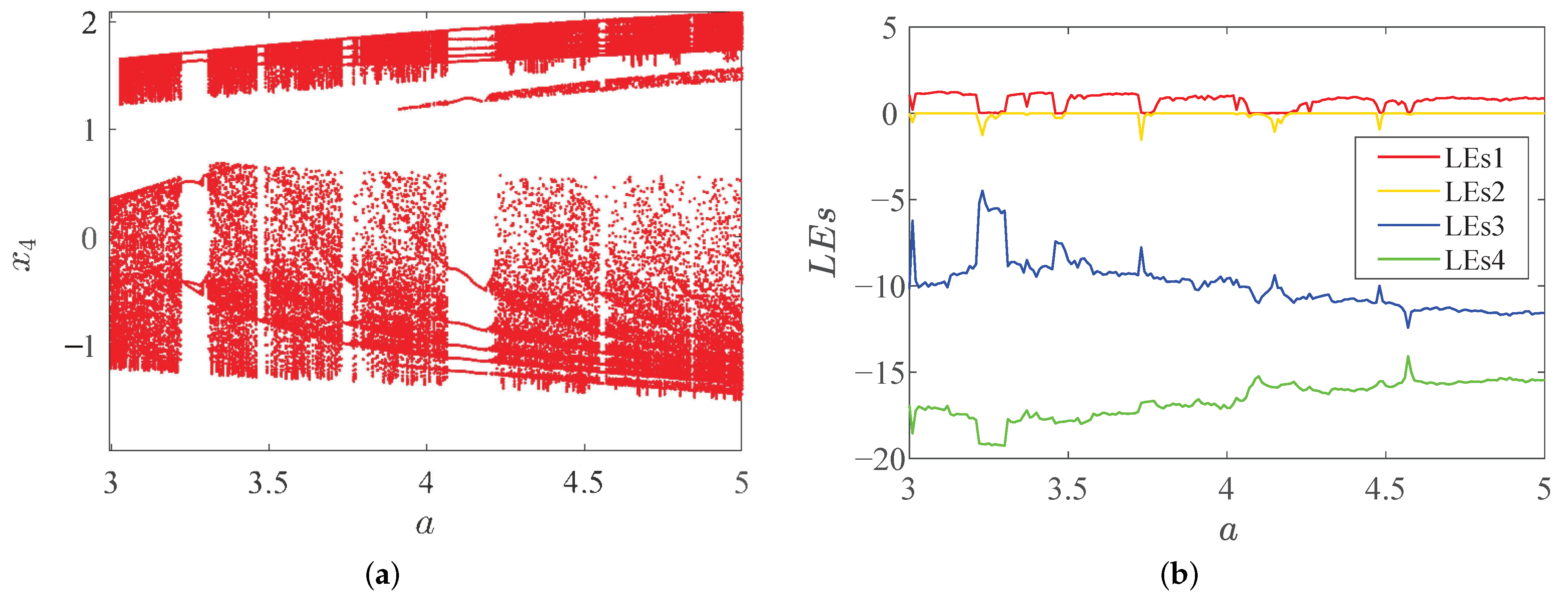
We fixed the order , the parameter a is used as a variable and selected the system parameters as , the initial value as , similarly. Then we obtained the bifurcation diagram and LEs diagram as show in Figure 7.
In Figure 7, it can be found that the system changes back and forth between a chaotic and periodic state, and that the dynamical behaviors are very rich.
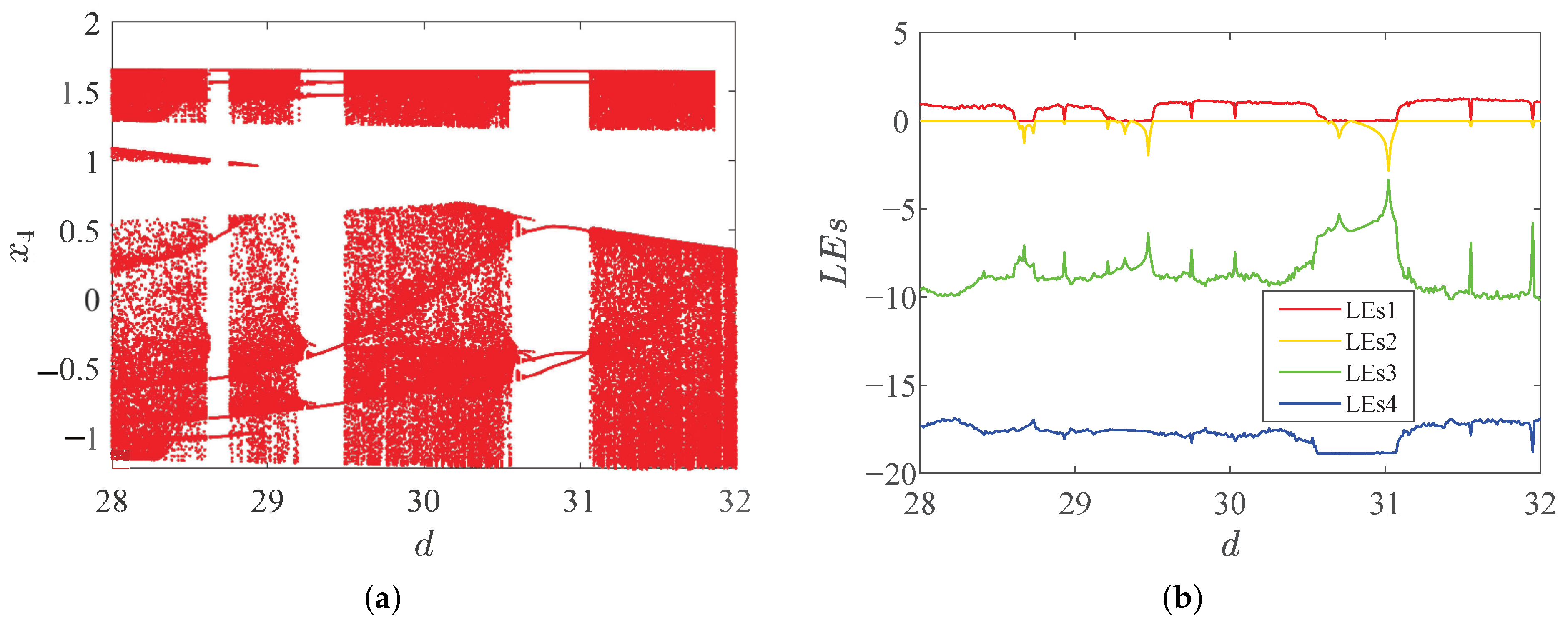
3.2.2. Parameter d as the Variable
Likewise, we fixed the order q, used the parameter d as a variable, and selected the system parameters as and the initial value as , similarly. Then, we obtained the bifurcation diagram and LEs diagram, as shown in Figure 8.
Regarding studying the dynamical behaviors of , Figure 8 shows the bifurcation diagram and LEs when selecting parameter d as the variable, and the numerical research of the system (15) indicates that, in addition to three periodic windows, i.e., , and , the system is in a chaotic state in most of the other parameter ranges.
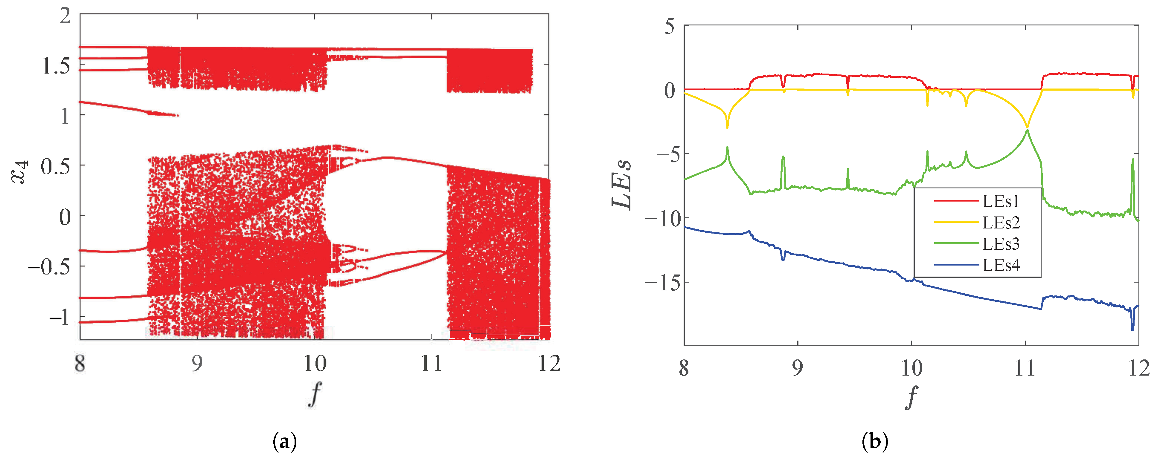
3.2.3. Parameter f as the Variable
Under the same parameters and conditions as the above analysis, is selected as the variable, and the bifurcation diagram and LEs diagram are shown in Figure 9.
3.3. Dynamical Analysis with Initial Value
Like before, we fixed the order , the parameter was selected as , and , and then we changed the initial value and , whereas and were not changed. Figure 10 and Figure 11 show the bifurcation diagram and LEs diagram of system (15) with and as variables.
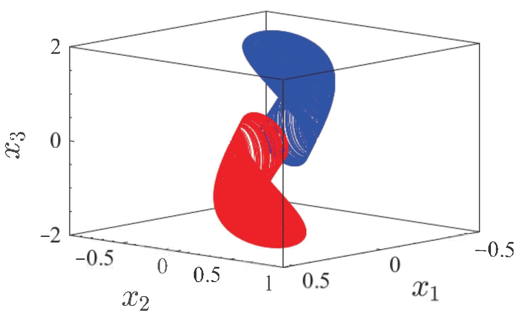
Figure 10 and Figure 11 show that the system (15) has symmetrical changes, i.e., when other conditions remain constant and the initial value changes, the system can emerge with coexisting attractors, as shown in Figure 12.
When some initial values of system (15) change, it can be found that the position of the attractor changes. This illustrates the multiple stability of the system, where it is just a dynamical property exhibited by the initial value space.
3.4. Offset Boosting
For a nonlinear system, adding a constant term after the uncoupled linear term of the variable that occurs only once in the system can offset the system (15). The constant is used as the control quantity, and the offset boosting can control the system offset. In Equation (15), variable satisfies the conditions of phase offset boosting. The constant term is added to the second dimension so we can obtain
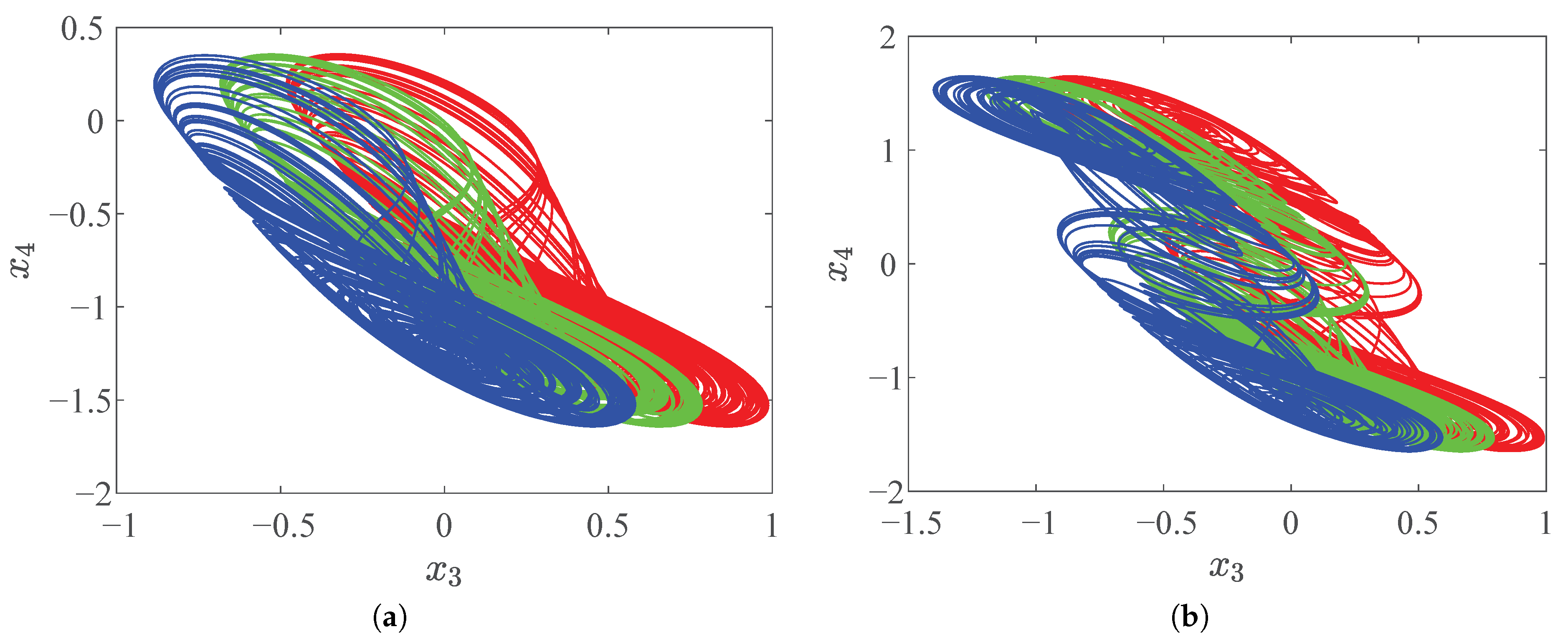
For the study of the offset boosting phenomenon, the parameters are consistent with the above, the initial values are , and the offset is set to 0, 0.2, and 0.4, respectively. When we change the fractional-orders q, we can find the offset boosting shown in Figure 13.
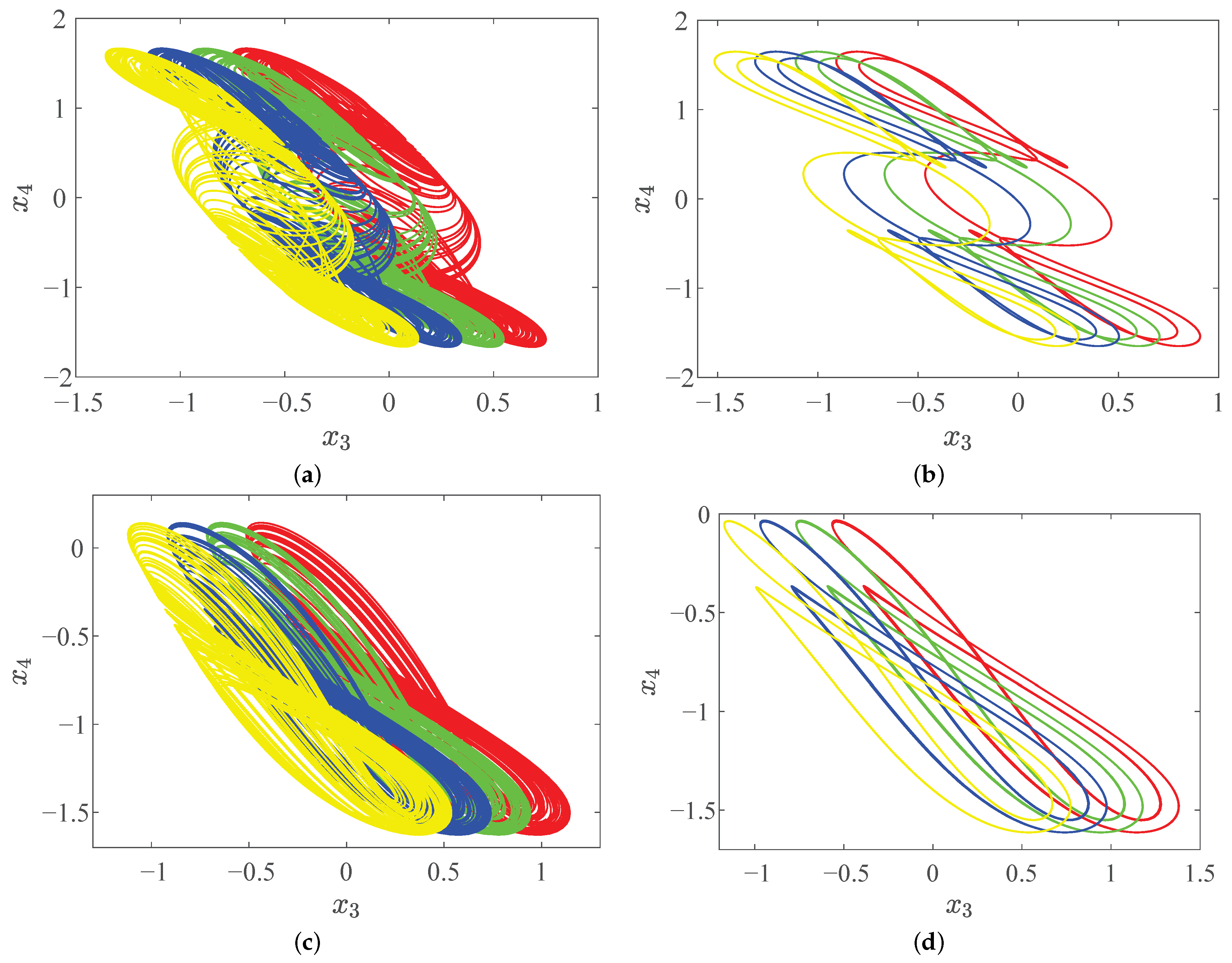
The system exhibits rich dynamical behaviors. To further study the offset boosting of system (15), under the same conditions, we only changed the value of f, in which, the offset was set to 0, 0.2, 0.4, and 0.6, and Figure 14 shows the position offset of the attractor under different parameters f.
As shown in Figure 14, when , the system is shown as being in a double-scroll chaotic state. When , the system remains in a double-scroll periodic state. When , the system is shown as being in a single-scroll chaotic state. When , the system remains in a single-scroll periodic state. Similarly, if we change the other parameters, we can find more offset boosting, indicating the rich and complex dynamical behaviors of the system.
4. System Circuit Implementation
4.1. Laplace Transform of Fractional-Order Memristor Circuit
Since it is impossib;le to perform a fractional differential calculation of a function or system directly in the time-domain, we can approximate the fractional-order operator using an integer-order operator as follows:
where the order , the initial value of the fractional-order system (15) is zero, and, in the time-domain transformation, the transfer function can be used to replace the fractional operator q. The Laplace transform can be used for system identification by using , where the maximum approximation error is 2 dB, and by considering the Bode diagram of the system (15). Thus, we can obtain
According to the Bode diagram (the maximum approximation error is 2 dB), we have
Here, let , , , , , , i.e., , and, by Equation (25), we can obtain
Let , , , , , , , , , , , , , , , ; then, Equation (27) can be further integrated into a 16-order integer-order differential equation, as shown in Table 3.
The initial values of ,; , ; , ; , are considered as zero throughout time-domain transformations, i.e., , , , , , , , , , , , , , , , in Table 3.
Therefore, a fractional-order system (15) can be converted into an integer-order system by time-frequency domain conversion and setting the step size to 0.1. It is a useful method for calculating fractional-order circuit systems using the Laplace transform. The fractional-order memristor analog circuit will then be implemented using the aforementioned method to validate the previous numerical simulation.
4.2. Circuit Simulation and FPGA Implementation
4.2.1. Analog Circuit Simulation
The analog circuit was designed as shown in Figure 15 in order to verify that the system (15) is functioning correctly. Multiplication was implemented by the AD633 multiplier, and the integral and addition operational amplifiers were implemented by TL082. All of the chips needed in the circuit were powered by V DC.
The principle equation of fractional-order memristor circuit is given according to the equivalent approximate fractional-order operator. According to the system (15), the equivalent circuit equation can be obtained as follows:
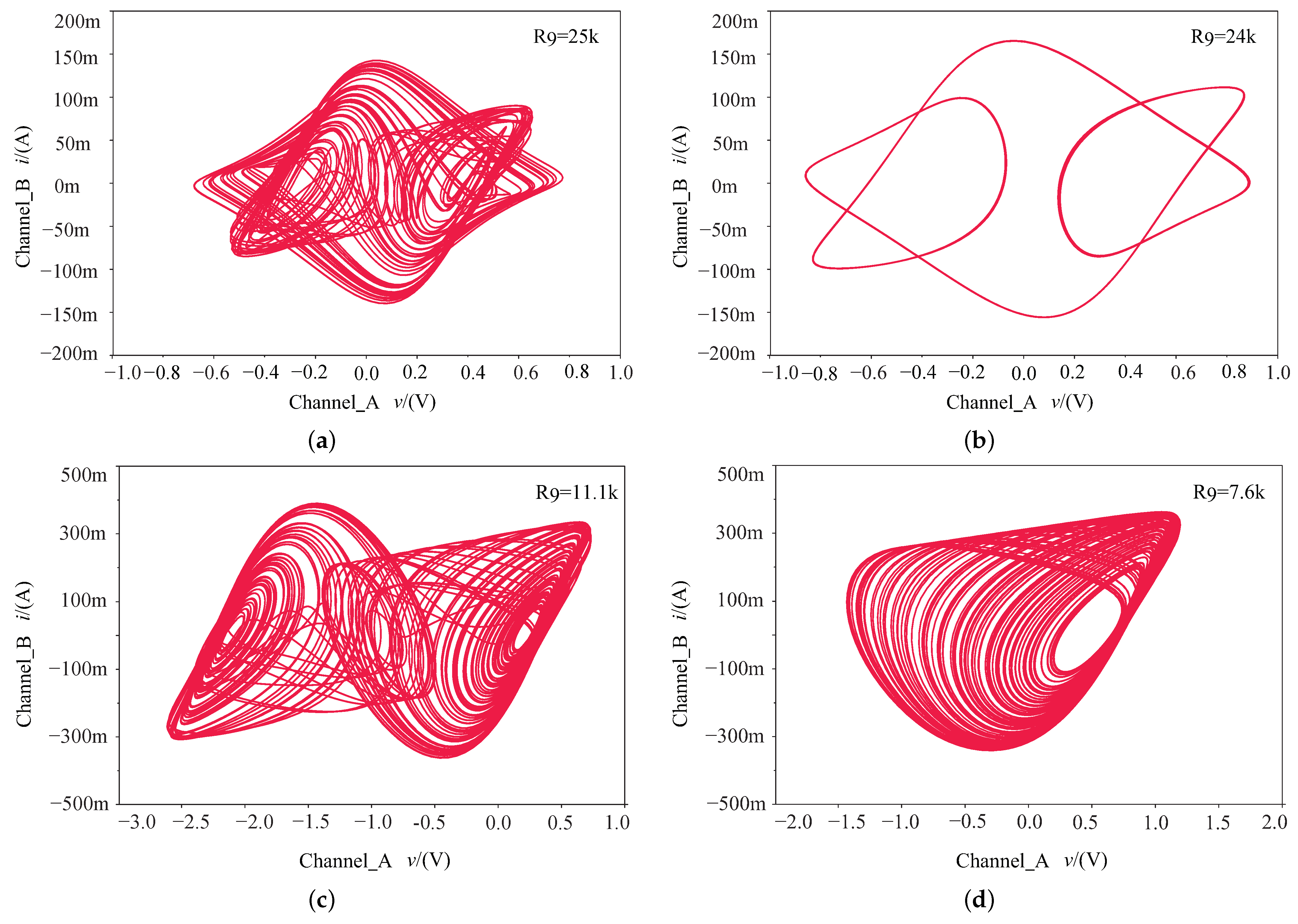
where , , , , , , , and so on are variable resistors corresponding to variable parameters in system (15). In Equation (28), represents the fractional-order modules in parallel on operational amplifiers U2, U5, U8, and U11. The circuit simulation results under different resistances are shown in Figure 16, and the resistance values, capacitance values, and corresponding parameters are shown in Figure 15. The simulation results of the circuit verify the symmetric and multistability of the system (15) well.
The numerical simulation results under different parameters f are consistent with the simulation results of the analog circuit under different resistances , which proves that the digital circuit can verify the chaotic behaviors of this system, including symmetric multi-stability.
4.2.2. FPGA System Implementation
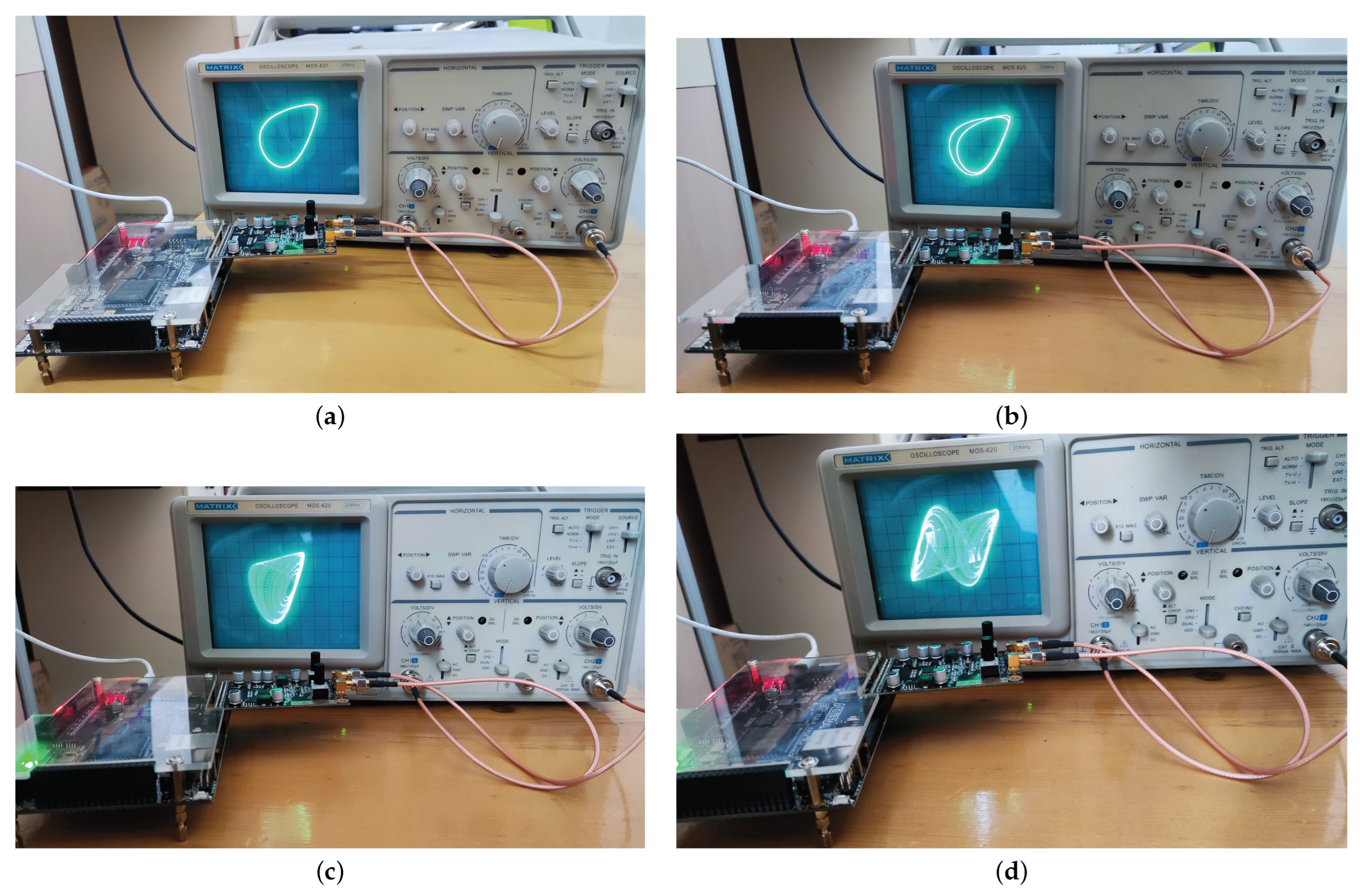
The selected system’s parameters are consistent with those of the aforementioned dynamics study: the step is , and the initial value is . The FPGA digital circuit of the system (15) was realized using the FPGA chip EPLC6Q240 of the Altera Cyclone4 series. To capture the system’s phase diagram on the digital oscilloscope, the only change was to the system parameter f, as shown in Figure 17.
In practice, the FPGA-based system design has received more and more attention. During the design of a fractional-order memristor system, modules are divided according to their functions at the top-level, and the relationship and cooperation mode between modules are planned. Verilog hardware is used at the bottom to realize the functions of each module. The clock frequency is 51.13 MHz, and the proportion of registers used is . The attractor phase diagram displayed by the oscilloscope in Figure 17 further verifies the existence of the system and the possibility of engineering applications.
4.3. Fractional-Order Memristor Control Circuit
Consider the master system of fractional-order memristor circuit (28). The slave system can be written as
Then, the error system can be written as . Thus, we can obtain
In this case, we give while setting the other controls to 0. Consequently, the system equation of the circuit controlled by a fractional-order memristor is as follows:
The values of each device in Figure 15 can be determined using the system parameters , , , , , and . Naturally, is the system’s equilibrium, and the Jacobian matrix following the circuit system’s linearization is
where . Then, we can determine that the eigenvalues are , , , and , respectively.
Lemma 1.
The stability lemma of fractional-order systems [40].
The commensurate system is stable if the following condition is satisfied:
where are eigenvalues, and the order q must satisfy
Accordingly, from Lemma 1, , i.e., , which satisfies Equation (33), occurs when the system is at zero equilibrium O. As a result, the system with can gradually stabilize to the equilibrium, and the fractional-order memristor feedback control circuit is designed as shown in Figure 18.
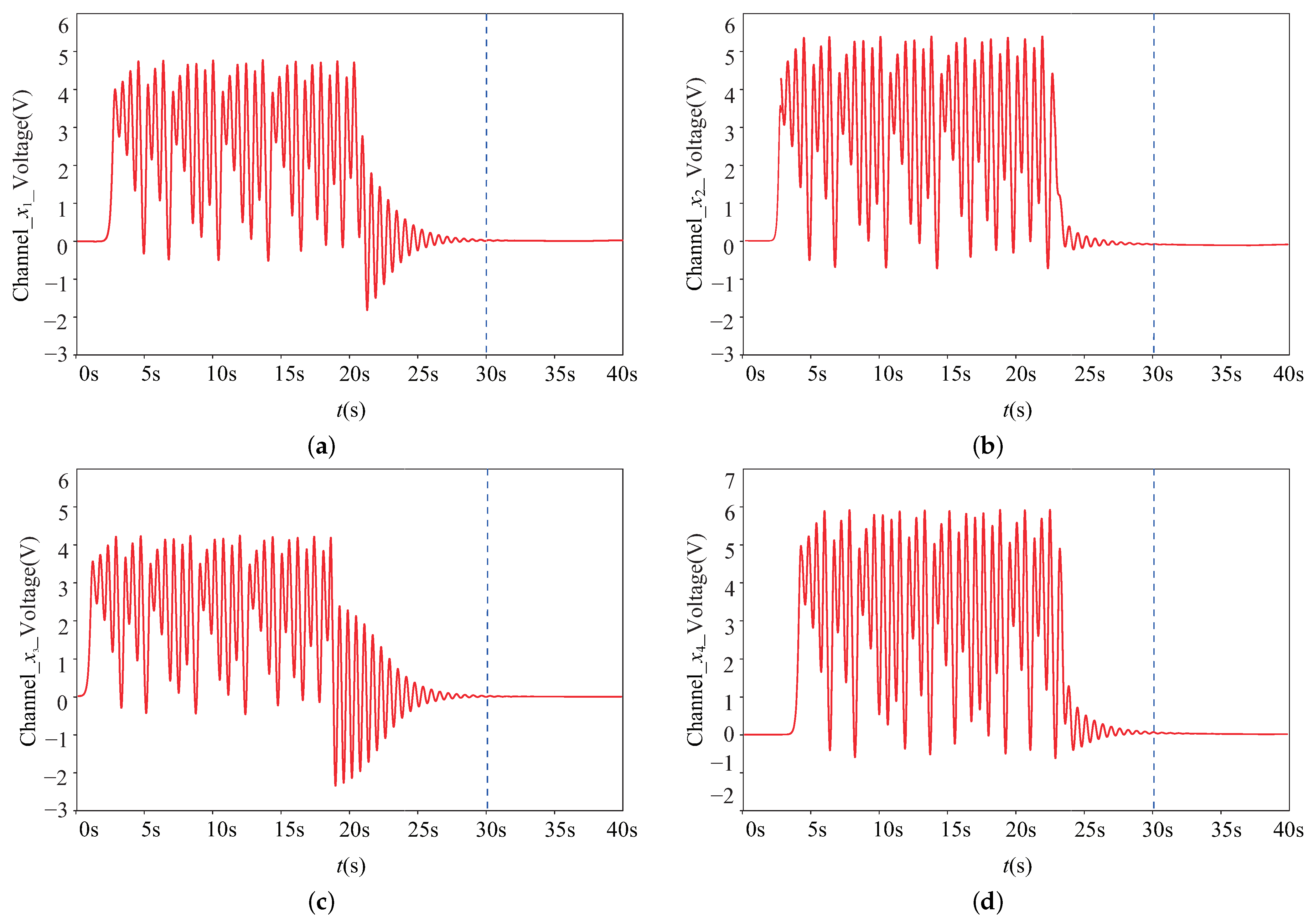
From the first channel of the feedback control circuit of Figure 18, when the resistance k and the switch on the control circuit is closed at time , the time-domain waveform of the state variable of the circuit experiment simulation of the memristor chaotic system feedback control circuit system is designed as shown in Figure 19.
According to the circuit experiment results of the time-domain waveform diagram of state variables (time responses of error system) in Figure 19, it can be found that its trajectory asymptotically converges to the origin by adding a feedback controller, which shows the control effect of the designed controller.
5. Conclusions
In this work, a novel fractional-order memristor system was established by integrating the fractional-order memristor into Chua’s circuit. Following that, the bifurcation diagram and LEs with system order, parameters, and initial values as independent variables were studied. The study revealed that altering these variables can cause the system to produce dynamical characteristics that are richer and more complex. In particular, the system exhibits periodic limit cycles and a single-scroll chaotic attractor; when the parameters and order of the system are changed, the system can generate a symmetric single-scroll chaotic attractor when the initial value is changed. Then, by adding a constant term after the decoupled linear term of the system, it was found that there is an offset boosting phenomenon in the system. Finally, the designed FPGA and analog circuit were established in accordance with the circuit equation to verify the numerical calculation results. The control circuit of the system was designed through the stability analysis of the equilibrium to satisfy the control requirements.
Based on the results obtained, the dynamics of a novel fractional-order memristor chaotic system studied in this paper are very rich due to the fractional-order operator, memristor, and offset boosting control, which provide a theoretical foundation for spread spectrum communication, pseudo-random sequence generators, and other practical engineering applications. Meanwhile, the possibility of the next work was further verified through the implementation of FPGA and analog circuits. Therefore, in the following work, we will summarize the shortcomings of this work, design and implement a fractional-order chaotic signal generator (floating point multiplier, floating point adder, fractional-order chaotic operation controller), and explore a novel fractional-order memristor chaotic system control scheme.
Author Contributions
Conceptualization, H.T. and J.L.; software, H.T.; validation, Z.W., F.X. and Z.C.; formal analysis, H.T.; writing—original draft preparation, H.T.; writing—review and editing, H.T. and Z.C.; visualization, J.L.; supervision, Z.W. All authors have read and agreed to the published version of the manuscript.
Funding
This work is supported by the National Natural Science Foundation of China (61973249), the Key Research and Development programs of Shaanxi Province (2021ZDLGY02-06), the Natural Science Basic Research Program of Shaanxi (2021JM-533, 2021JQ-880, 2020JM-646), the Innovation Capability Support Program of Shaanxi (2018GHJD-21), the Qin Chuangyuan Project (2021QCYRC4-49), the Support Plan for Sanqin Scholars Innovation Team in Shaanxi Province of China, the National Defense Science and Technology Key Laboratory Fund Project (6142101210202), the Qinchuangyuan Scientist+Engineer (2022KXJ-169), the Scientific Research Program Funded by Shaanxi Provincial Education Department (21JK0960), the Scientific Research Fund for High-Level Talents of Xijing University (XJ21B01), and the Scientific Research Foundation of Xijing University (XJ210203).
Institutional Review Board Statement
Not applicable.
Informed Consent Statement
Not applicable.
Data Availability Statement
Not applicable.
Acknowledgments
The author acknowledges the referees and the editor for carefully reading this paper and giving many helpful comments. The authors also express their gratitude to the reviewers for their insightful comments.
Conflicts of Interest
The authors declare no conflict of interest.
Appendix A
The nonlinear term of the Equation (21) is decomposition, which can be obtained as
where is the initial value of Equation (A1), and , , . Let , , , ; then, from of Equation (20) and the properties of fractional integral operators, the is
Assign the coefficient to the variable, i.e.,
Then, from of Equation (20) and the properties of fractional integral operators, we can obtain the equation for , and, in the same way, we obtain
and the coefficients of the next three terms are
References
- Lorenz, E.N. Deterministic nonperiodic flow. J. Atmos. Sci. 1963, 20, 130–141. [Google Scholar] [CrossRef]
- Rössler, O.E. An equation for continuous chaos. Phys. Lett. 1976, 57, 397–398. [Google Scholar] [CrossRef]
- Chen, G.; Ueta, T. Yet another chaotic attractor. Int. J. Bifurc. Chaos 1999, 9, 1465–1466. [Google Scholar] [CrossRef]
- Lü, J.; Chen, G. A new chaotic attractor coined. Int. J. Bifurc. Chaos 2002, 12, 659–661. [Google Scholar] [CrossRef] [Green Version]
- Ma, C.; Mou, J.; Xiong, L.; Banerjee, S.; Liu, T.; Han, X. Dynamical analysis of a new chaotic system: Asymmetric multistability, offset boosting control and circuit realization. Nonlinear Dyn. 2021, 103, 2867–2880. [Google Scholar] [CrossRef]
- Zhou, L.; You, Z.; Tang, Y. A new chaotic system with nested coexisting multiple attractors and riddled basins. Chaos Solitons Fractals 2021, 148, 111057. [Google Scholar] [CrossRef]
- Tian, H.; Wang, Z.; Zhang, P.; Chen, M.; Wang, Y. Dynamic analysis and robust control of a chaotic system with hidden attractor. Complexity 2021, 2021, 8865522. [Google Scholar] [CrossRef]
- Wang, Z.; Wei, Z.; Sun, K.; He, S.; Wang, H.; Xu, Q.; Chen, M. Chaotic flows with special equilibria. Eur. Phys. J. Spec. Top. 2020, 229, 905–919. [Google Scholar] [CrossRef]
- Tian, H.; Wang, Z.; Zhang, H.; Cao, Z.; Zhang, P. Dynamical analysis and fixed-time synchronization of a chaotic system with hidden attractor and a line equilibrium. Eur. Phys. J. Spec. Top. 2022, 231, 2455–2466. [Google Scholar] [CrossRef]
- Li, C.; Rajagopal, K.; Nazarimehr, F.; Liu, Y. A non-autonomous chaotic system with no equilibrium. Integration 2021, 79, 143–156. [Google Scholar] [CrossRef]
- Zhang, R.; Xi, X.; Tian, H.; Wang, Z. Dynamical Analysis and Finite-Time Synchronization for a Chaotic System with Hidden Attractor and Surface Equilibrium. Axioms 2022, 11, 579. [Google Scholar] [CrossRef]
- Ye, G.; Pan, C.; Huang, X.; Mei, Q. An efficient pixel-level chaotic image encryption algorithm. Nonlinear Dyn. 2018, 94, 745–756. [Google Scholar] [CrossRef]
- Ahmad, I.; Ouannas, A.; Shafiq, M.; Pham, V.T.; Baleanu, D. Finite-time stabilization of a perturbed chaotic finance model. J. Adv. Res. 2021, 32, 1–14. [Google Scholar] [CrossRef] [PubMed]
- Qin, C.; Sun, K.; He, S. Characteristic analysis of fractional-order memristor-based hypogenetic jerk system and its DSP implementation. Electronics 2021, 10, 841. [Google Scholar] [CrossRef]
- Chua, L. Memristor-the missing circuit element. IEEE Trans. Circuit Theory 1971, 18, 507–519. [Google Scholar] [CrossRef]
- Strukov, D.B.; Snider, G.S.; Stewart, D.R.; Williams, R.S. The missing memristor found. Nature 2008, 453, 80–83. [Google Scholar] [CrossRef]
- Lai, Q.; Wan, Z.; Kuate, P.D.K.; Fotsin, H. Coexisting attractors, circuit implementation and synchronization control of a new chaotic system evolved from the simplest memristor chaotic circuit. Commun. Nonlinear Sci. Numer. Simul. 2020, 89, 105341. [Google Scholar] [CrossRef]
- Rajagopal, K.; Kacar, S.; Wei, Z.; Duraisamy, P.; Kifle, T.; Karthikeyan, A. Dynamical investigation and chaotic associated behaviors of memristor Chua’s circuit with a non-ideal voltage-controlled memristor and its application to voice encryption. Aeu-Int. J. Electron. Commun. 2019, 107, 183–191. [Google Scholar] [CrossRef]
- Xie, W.; Wang, C.; Lin, H. A fractional-order multistable locally active memristor and its chaotic system with transient transition, state jump. Nonlinear Dyn. 2021, 104, 4523–4541. [Google Scholar] [CrossRef]
- Qi, Y.; Wu, C.; Zhang, Q.; Yan, K.; Wang, H. Complex dynamics behavior analysis of a new chaotic system based on fractional-order memristor. J. Phys. Conf. Ser. 2021, 1861, 012114. [Google Scholar] [CrossRef]
- Liu, J.; Wang, Z.; Chen, M.; Zhang, P.; Yang, R.; Yang, B. Chaotic system dynamics analysis and synchronization circuit realization of fractional-order memristor. Eur. Phys. J. Spec. Top. 2022, 231, 3095–3107. [Google Scholar] [CrossRef]
- Volos, C.K.; Pham, V.T.; Nistazakis, H.E.; Stouboulos, I.N. A dream that has come true: Chaos from a nonlinear circuit with a real memristor. Int. J. Bifurc. Chaos 2020, 30, 2030036. [Google Scholar] [CrossRef]
- Wang, Z.; Baruni, S.; Parastesh, F.; Jafari, S.; Ghosh, D.; Perc, M.; Hussain, I. Chimeras in an adaptive neuronal network with burst-timing-dependent plasticity. Neurocomputing 2020, 406, 117–126. [Google Scholar] [CrossRef]
- Wang, Z.; Parastesh, F.; Rajagopal, K.; Hamarash, I.I.; Hussain, I. Delay-induced synchronization in two coupled chaotic memristive Hopfield neural networks. Chaos Solitons Fractals 2020, 134, 109702. [Google Scholar] [CrossRef]
- Liang, H.; Wang, Z.; Yue, Z.; Lu, R. Generalized synchronization and control for incommensurate fractional unified chaotic system and applications in secure communication. Kybernetika 2012, 48, 190–205. [Google Scholar]
- Gu, S.; Peng, Q.; Leng, X.; Du, B. A novel non-equilibrium memristor-based system with multi-wing attractors and multiple transient transitions. Chaos Interdiscip. Nonlinear Sci. 2021, 31, 033105. [Google Scholar] [CrossRef]
- Liao, H.; Ding, Y.; Wang, L. Adomian decomposition algorithm for studying incommensurate fractional-order memristor-based Chua’s system. Int. J. Bifurc. Chaos 2018, 28, 1850134. [Google Scholar] [CrossRef]
- Mou, J.; Sun, K.; Wang, H.; Ruan, J. Characteristic analysis of fractional-order 4D hyperchaotic memristive circuit. Math. Probl. Eng. 2017, 2017, 2313768. [Google Scholar] [CrossRef] [Green Version]
- Wu, J.; Wang, G.; Iu, H.H.C.; Shen, Y.; Zhou, W. A nonvolatile fractional order memristor model and its complex dynamics. Entropy 2019, 21, 955. [Google Scholar] [CrossRef] [Green Version]
- Yu, Y.; Bao, H.; Shi, M.; Bao, B.; Chen, Y.; Chen, M. Complex dynamical behaviors of a fractional-order system based on a locally active memristor. Complexity 2019, 2019, 2051053. [Google Scholar] [CrossRef]
- Chen, C.; Chen, J.; Bao, H.; Chen, M.; Bao, B. Coexisting multi-stable patterns in memristor synapse-coupled Hopfield neural network with two neurons. Nonlinear Dyn. 2019, 95, 3385–3399. [Google Scholar] [CrossRef]
- Bao, H.; Wang, N.; Bao, B.; Chen, M.; Jin, P.; Wang, G. Initial condition-dependent dynamics and transient period in memristor-based hypogenetic jerk system with four line equilibria. Commun. Nonlinear Sci. Numer. Simul. 2018, 57, 264–275. [Google Scholar] [CrossRef]
- Sahin, M.; Taskiran, Z.C.; Guler, H.; Hamamci, S. Simulation and implementation of memristive chaotic system and its application for communication systems. Sens. Actuators A Phys. 2019, 290, 107–118. [Google Scholar] [CrossRef]
- Wang, S. Dynamical analysis of memristive unified chaotic system and its application in secure communication. IEEE Access 2018, 6, 66055–66061. [Google Scholar] [CrossRef]
- Haliuk, S.; Krulikovskyi, O.; Vovchuk, D.; Corinto, F. Memristive structure-based chaotic system for prng. Symmetry 2022, 14, 68. [Google Scholar] [CrossRef]
- Han, S.M.; Takasawa, T.; Yasutomi, K.; Aoyama, S.; Kagawa, K.; Kawahito, S. A time-of-flight range image sensor with background canceling lock-in pixels based on lateral electric field charge modulation. IEEE J. Electron Devices Soc. 2014, 3, 267–275. [Google Scholar] [CrossRef]
- Sebastian, A.; Le Gallo, M.; Khaddam-Aljameh, R.; Eleftheriou, E. Memory devices and applications for in-memory computing. Nat. Nanotechnol. 2020, 15, 529–544. [Google Scholar] [CrossRef]
- Khanzadeh, A.; Mohammadzaman, I. Comment on “Fractional-order fixed-time nonsingular terminal sliding mode synchronization and control of fractional-order chaotic systems”. Nonlinear Dyn. 2018, 94, 3145–3153. [Google Scholar] [CrossRef]
- Podlubny, I. Fractional-order systems and PI/sup/spl lambda//D/sup/spl mu//-controllers. IEEE Trans. Autom. Control 1999, 44, 208–214. [Google Scholar] [CrossRef]
- Matignon, D. Stability properties for generalized fractional differential systems. In ESAIM: Proceedings; EDP Sciences: Paris, France, 1998; Volume 5, pp. 145–158. [Google Scholar]
Figure 1.
Characteristic comparison of fractional-order memristor. (a) Memristor hysteresis loops of different orders q; (b) memristor hysteresis loops of different frequencies ; (c) memristor hysteresis loops of different voltage amplitudes ; (d) time-domain diagram of the change in memristance in different orders q; (e) time-domain diagram of output current at different orders q; (f) time-domain diagram of output power under different orders q;

Figure 2.
Fractional-order memristor chaotic circuit.

Figure 3.
Simulation diagram of fractional-order memristor hysteresis loop circuit in plane. (a) Different amplitudes A; (b) different frequencies f.
Figure 3.
Simulation diagram of fractional-order memristor hysteresis loop circuit in plane. (a) Different amplitudes A; (b) different frequencies f.
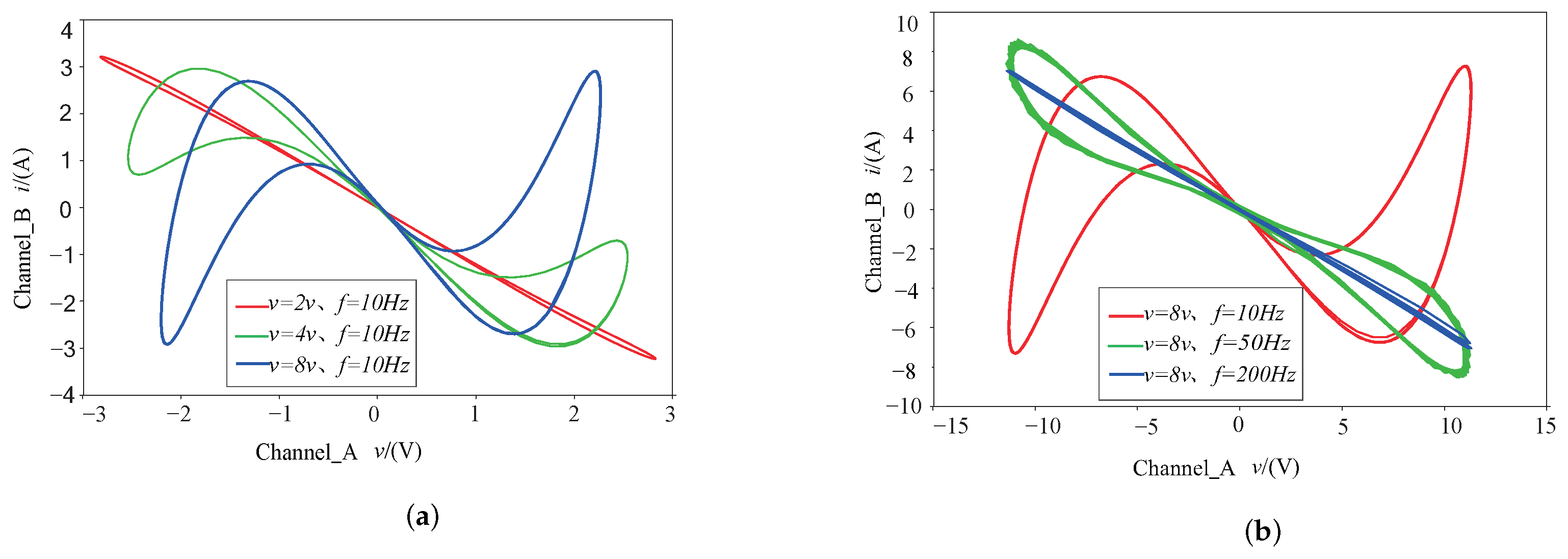
Figure 4.
The system plane phase diagram of changing the parameter f of system (15). (a) ; (b) ; (c) ; (d) .
Figure 4.
The system plane phase diagram of changing the parameter f of system (15). (a) ; (b) ; (c) ; (d) .
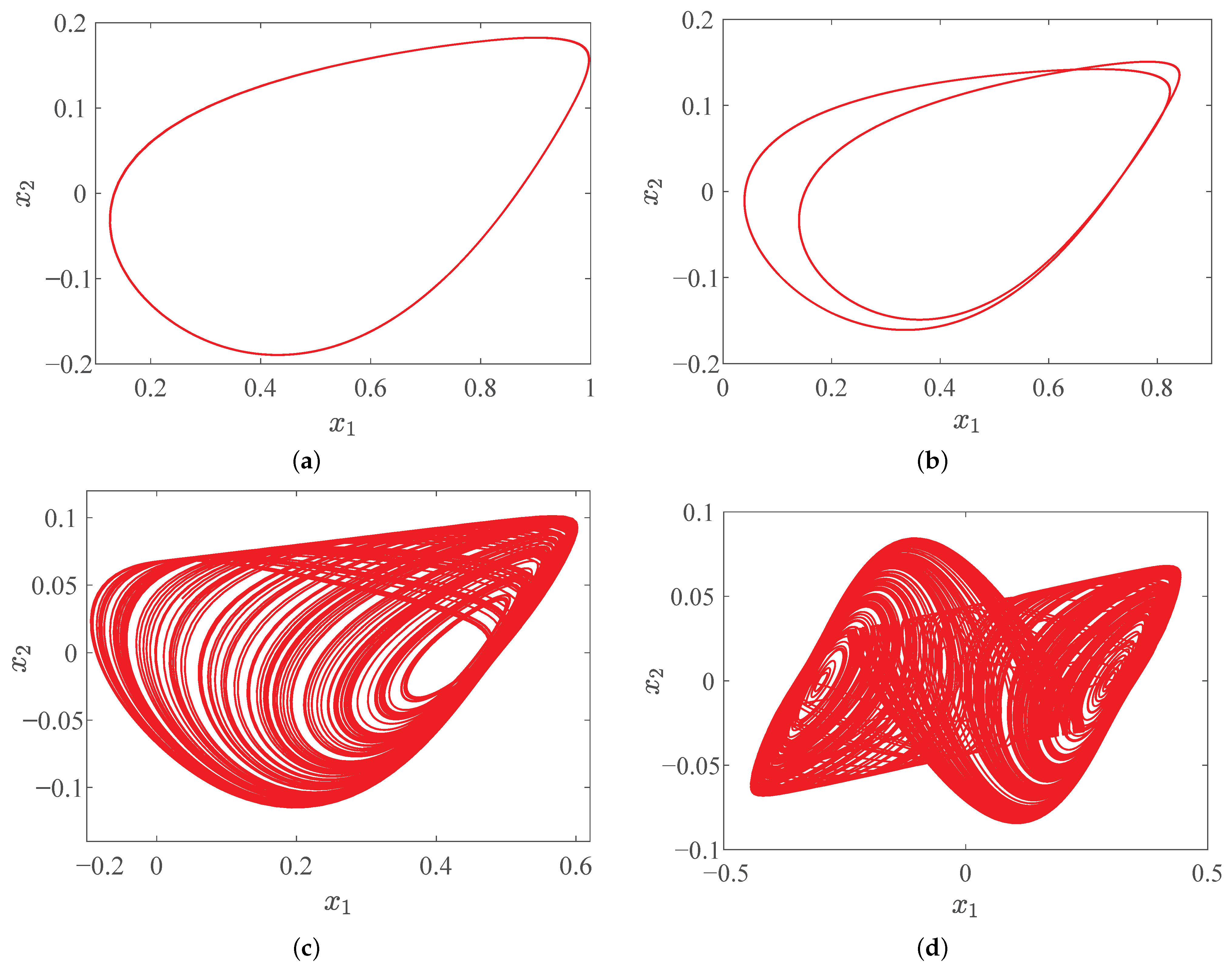
Figure 5.
Dynamical behaviors with fractional orders q of system (15). (a) Bifurcation diagram; (b) LEs.
Figure 5.
Dynamical behaviors with fractional orders q of system (15). (a) Bifurcation diagram; (b) LEs.
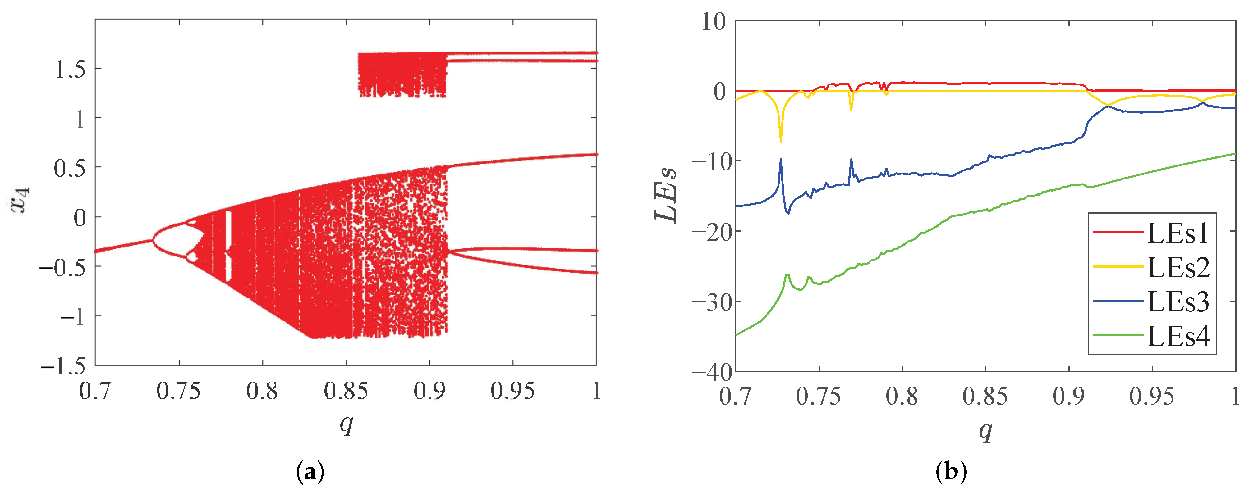
Figure 6.
Phase diagrams of system (15) in plane. (a) Period-1 of ; (b) period-2 of ; (c) period-4 of ; (d) single-scroll attractor of ; (e) double-scroll chaotic attractor of ; (f) period-2 of .
Figure 6.
Phase diagrams of system (15) in plane. (a) Period-1 of ; (b) period-2 of ; (c) period-4 of ; (d) single-scroll attractor of ; (e) double-scroll chaotic attractor of ; (f) period-2 of .
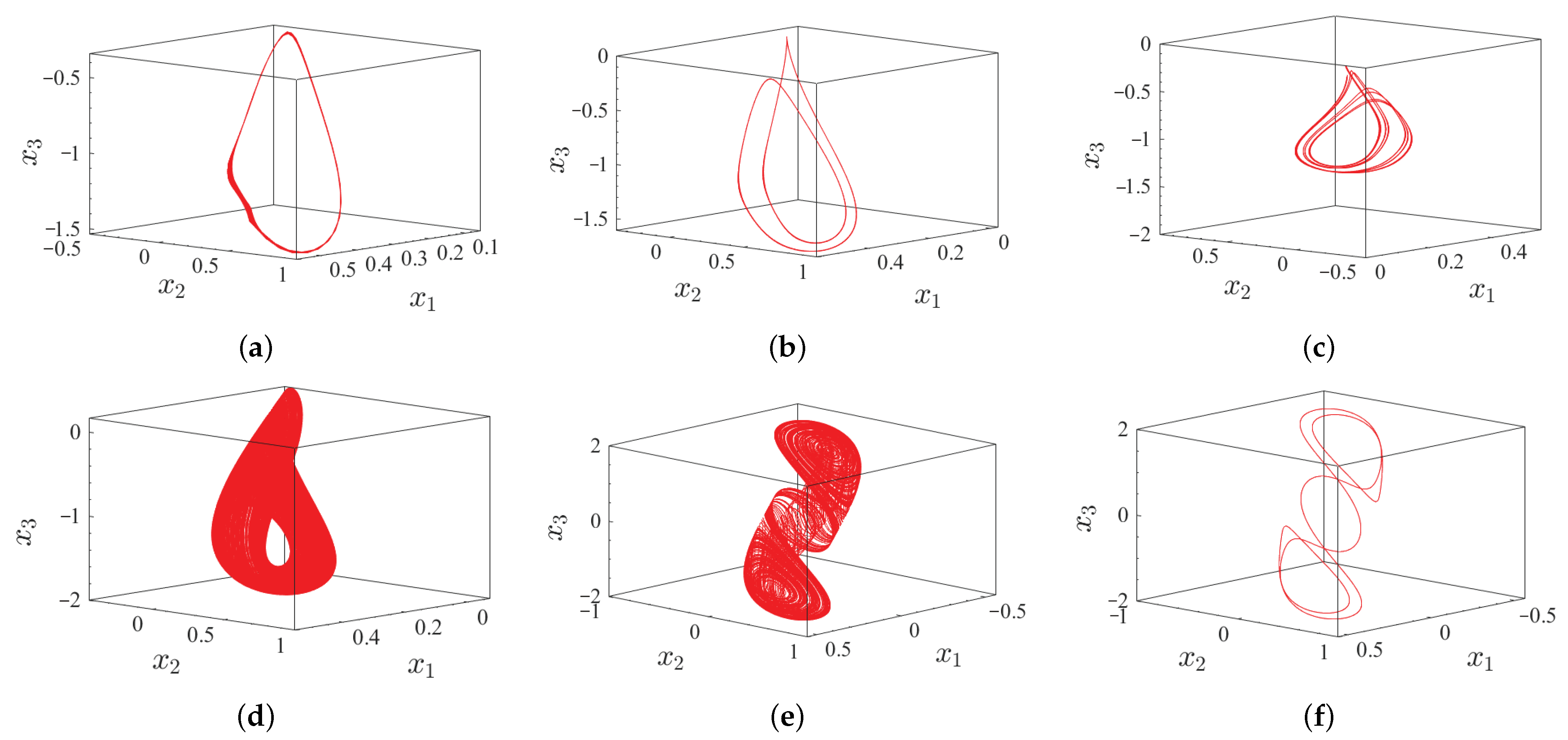
Figure 7.
Dynamical behaviors with different parameter a of system (15). (a) Bifurcation diagram; (b) LEs.
Figure 7.
Dynamical behaviors with different parameter a of system (15). (a) Bifurcation diagram; (b) LEs.

Figure 8.
Dynamical behaviors with different parameter d of system (15). (a) Bifurcation diagram; (b) LEs.
Figure 8.
Dynamical behaviors with different parameter d of system (15). (a) Bifurcation diagram; (b) LEs.

Figure 9.
Dynamical behaviors with different parameter f of system (15). (a) Bifurcation diagram; (b) LEs.
Figure 9.
Dynamical behaviors with different parameter f of system (15). (a) Bifurcation diagram; (b) LEs.

Figure 10.
Dynamical behaviors with changes in initial value of system (15). (a) Bifurcation diagram; (b) LEs.
Figure 10.
Dynamical behaviors with changes in initial value of system (15). (a) Bifurcation diagram; (b) LEs.
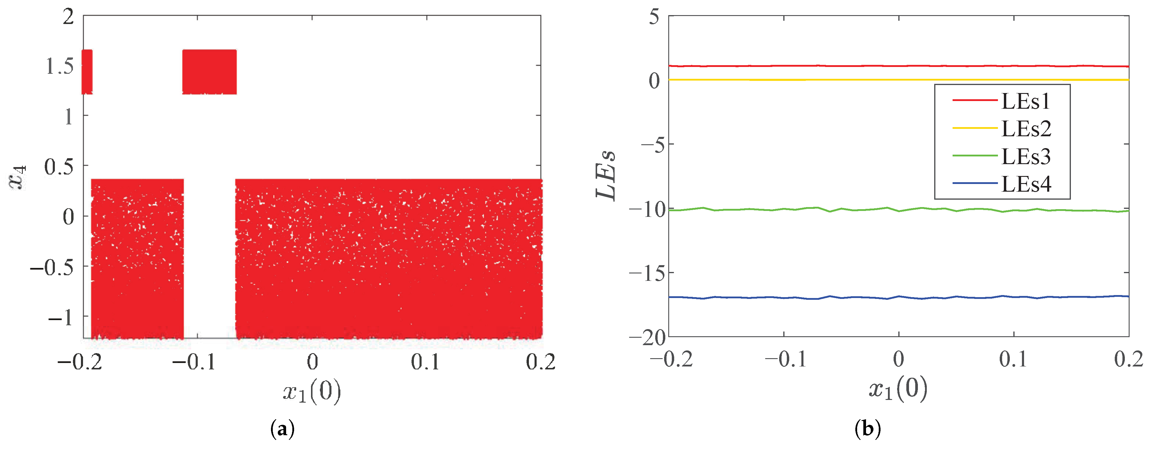
Figure 11.
Dynamical behaviors with changes in initial value of system (15). (a) Bifurcation diagram; (b) LEs.
Figure 11.
Dynamical behaviors with changes in initial value of system (15). (a) Bifurcation diagram; (b) LEs.
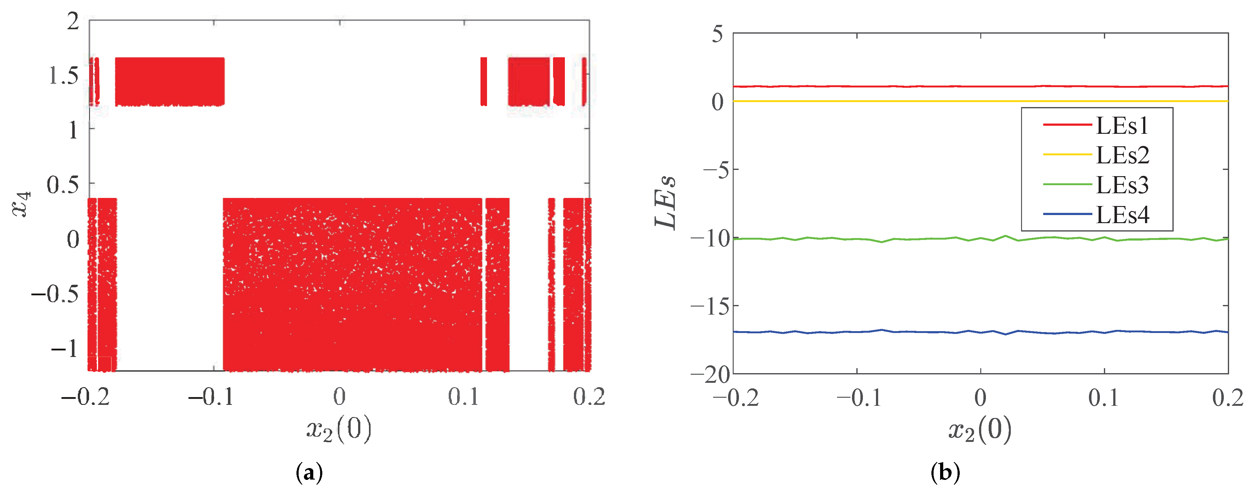
Figure 12.
Symmetric coexistence chaotic attractors of system (15). (Red is and blue is ).
Figure 12.
Symmetric coexistence chaotic attractors of system (15). (Red is and blue is ).

Figure 13.
Offset boosting ( (red), (green), (blue)) with change in fractional-order q. (a) , (b) .

Figure 14.
Offset boosting ( (red), (green), (blue), (yellow)) with parameter f change. (a) ; (b) ; (c) ; (d) .
Figure 14.
Offset boosting ( (red), (green), (blue), (yellow)) with parameter f change. (a) ; (b) ; (c) ; (d) .

Figure 15.
Circuit diagram of fractional-order memristor system (15).
Figure 15.
Circuit diagram of fractional-order memristor system (15).
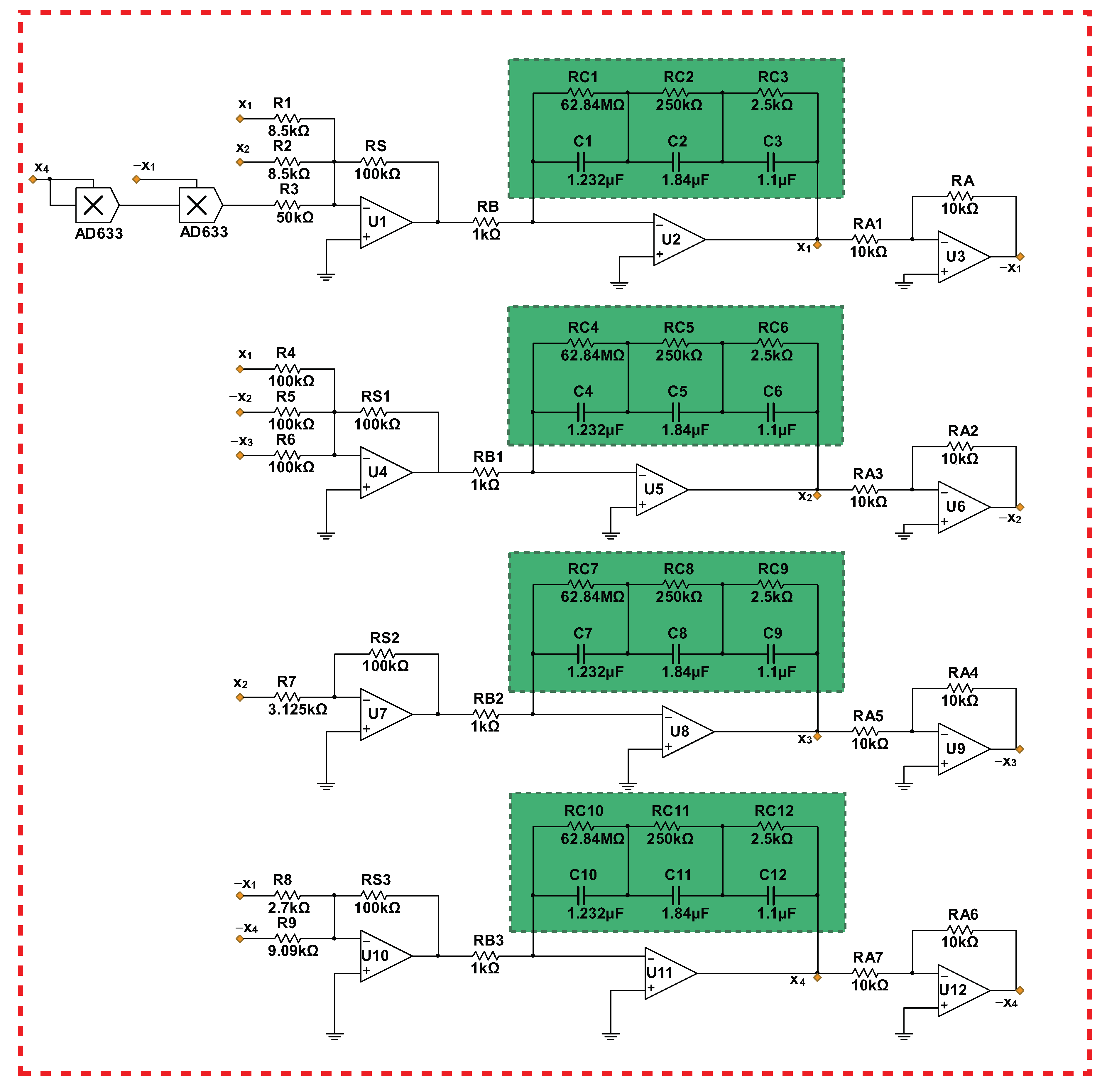
Figure 16.
Circuit simulation under different resistances in plane. (a) Single-scroll periodic-1 limit cycle with k; (b) single-scroll periodic-2 limit cycle with k; (c) single-scroll chaotic attractor with k; (d) symmetric single-scroll chaotic attractor with k.
Figure 16.
Circuit simulation under different resistances in plane. (a) Single-scroll periodic-1 limit cycle with k; (b) single-scroll periodic-2 limit cycle with k; (c) single-scroll chaotic attractor with k; (d) symmetric single-scroll chaotic attractor with k.

Figure 17.
Experimental results of FPGA digital circuits of the fractional-order memristor system (15). (a) Single-scroll periodic-1 limit cycle with ; (b) single-scroll periodic-2 limit cycle with ; (c) single-scroll chaotic attractor with ; (d) symmetric single-scroll chaotic attractor with .
Figure 17.
Experimental results of FPGA digital circuits of the fractional-order memristor system (15). (a) Single-scroll periodic-1 limit cycle with ; (b) single-scroll periodic-2 limit cycle with ; (c) single-scroll chaotic attractor with ; (d) symmetric single-scroll chaotic attractor with .

Figure 18.
Schematic diagram of feedback control circuit of the first channel.
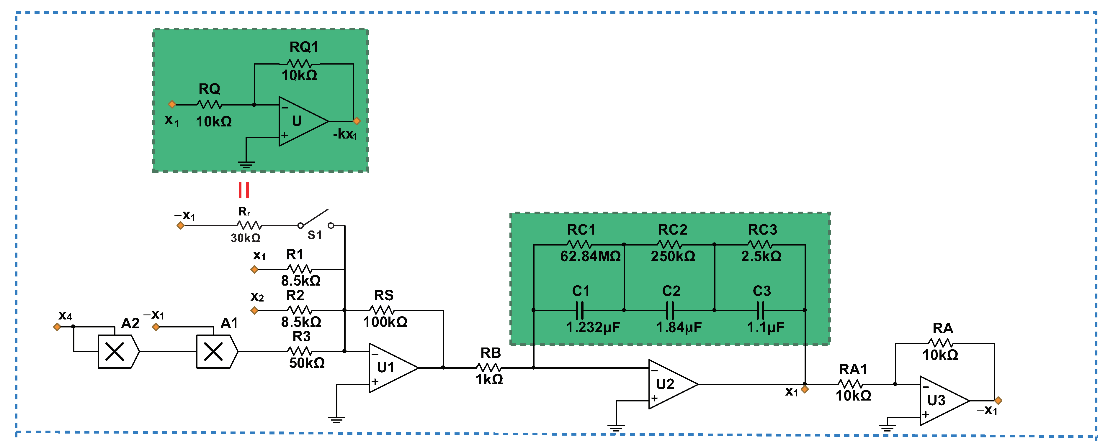
Figure 19.
Time-domain waveforms of state variables of the system (28). (a) plane; (b) plane; (c) plane; (d) plane.
Figure 19.
Time-domain waveforms of state variables of the system (28). (a) plane; (b) plane; (c) plane; (d) plane.

Table 1.
Value of circuit elements of fractional-order memristor.
| Circuit Element | Physical Meaning of Parameters | Parameter Value |
|---|---|---|
| resistance | 10k | |
| resistance | 62 k | |
| resistance | 100 k | |
| resistance | 125 k | |
| capacitance | 1 nF |
Table 2.
Dynamical behaviors of system (15) as the order q changes.
Table 2.
Dynamical behaviors of system (15) as the order q changes.
| q | Dynamical Properties | Phase Diagrams |
|---|---|---|
| (0.700,0.748) | periodic-1 | Figure 6a |
| (0.748,0.754) | periodic-2 | Figure 6b |
| (0.754,0.780) | periodic-4 | Figure 6c |
| (0.780,0.850) | chaotic | Figure 6d |
| (0.850,0.910) | chaotic | Figure 6e |
| (0.910,1.000) | periodic-2 | Figure 6f |
Table 3.
Sixteen-order integer-order differential equation of system (27).
Table 3.
Sixteen-order integer-order differential equation of system (27).
Disclaimer/Publisher’s Note: The statements, opinions and data contained in all publications are solely those of the individual author(s) and contributor(s) and not of MDPI and/or the editor(s). MDPI and/or the editor(s) disclaim responsibility for any injury to people or property resulting from any ideas, methods, instructions or products referred to in the content. |
© 2022 by the authors. Licensee MDPI, Basel, Switzerland. This article is an open access article distributed under the terms and conditions of the Creative Commons Attribution (CC BY) license (https://creativecommons.org/licenses/by/4.0/).
Share and Cite
MDPI and ACS Style
Tian, H.; Liu, J.; Wang, Z.; Xie, F.; Cao, Z. Characteristic Analysis and Circuit Implementation of a Novel Fractional-Order Memristor-Based Clamping Voltage Drift. Fractal Fract. 2023, 7, 2. https://doi.org/10.3390/fractalfract7010002
AMA Style
Tian H, Liu J, Wang Z, Xie F, Cao Z. Characteristic Analysis and Circuit Implementation of a Novel Fractional-Order Memristor-Based Clamping Voltage Drift. Fractal and Fractional. 2023; 7(1):2. https://doi.org/10.3390/fractalfract7010002
Chicago/Turabian StyleTian, Huaigu, Jindong Liu, Zhen Wang, Fei Xie, and Zelin Cao. 2023. "Characteristic Analysis and Circuit Implementation of a Novel Fractional-Order Memristor-Based Clamping Voltage Drift" Fractal and Fractional 7, no. 1: 2. https://doi.org/10.3390/fractalfract7010002