
Quadratic Admissibility for a Class of LTI Uncertain Singular Fractional-Order Systems with 0 < α < 2


1
College of Sciences, Northeastern University, Shenyang 110819, China
2
INSA Centre Val de Loire, Université d’Orléans, PRISME EA 4229, CEDEX, 18022 Bourges, France
3
School of Electrical and Electronic Engineering, The University of Adelaide, Adelaide, SA 5005, Australia
*
Author to whom correspondence should be addressed.
Fractal Fract. 2023, 7(1), 1; https://doi.org/10.3390/fractalfract7010001
Submission received: 9 November 2022
/
Revised: 9 December 2022
/
Accepted: 16 December 2022
/
Published: 20 December 2022
(This article belongs to the Special Issue Applications of Fractional Operator in Image Processing and Stability of Control Systems)
Abstract
:This paper provides a unified framework for the admissibility of a class of singular fractional-order systems with a given fractional order in the interval . These necessary and sufficient conditions are derived in terms of linear matrix inequalities (LMIs). The considered fractional orders range from 0 to 2 without separating the ranges into and to discuss the admissibility. Moreover, the uncertain system with the fractional order in the interval is norm-bounded. The quadratic admissibility and general quadratic stability of the system are analyzed, and the equivalence between the two is proved. All the above can be expressed in terms of strict LMIs to avoid any singularity problem in the solution. Finally, the effectiveness of the method is illustrated by three numerical examples.
1. Introduction
Fractional-order systems (FOSs) have received extensive attention in the field of natural science and applied engineering [1,2] in recent years and have gradually become a research hot spot because of their many practical backgrounds and engineering requirements. In order to conform to the actual research situation, the current research expands results from classical calculus [3,4] to fractional calculus [5,6]. Indeed, FOSs are used to represent the nonclassical phenomena of various types of physical systems; FOSs have gradually become the main research object in the control field.
For all systems, stability is a prerequisite for the proper functioning of control systems in practical applications, let alone in FOSs. However, the stability analysis of FOSs [7,8] cannot be derived directly from integer-order systems (IOSs) [9,10] due to the complexity of their operators, and thus the stability of FOSs has become a hot topic of discussion in recent years. Li and Yu [11,12] proposed the definition of the Mittag–Leffler stability and introduced the fractional Lyapunov direct method to study the stability of fractional-order nonlinear dynamical systems. Lu and Chen [13] discussed the system matrix with interval uncertainties and analyzed the problem of the robust asymptotic stability of systems, where the order is in the interval (0, 1). In [14], Semary confirmed the relationship between the stability of FOSs and the number of poles and investigated the stability of these systems by discussing the time-domain response based on the Mittag–Leffler function. Alagoz [15] analyzed the stability of FOSs by studying the root trajectories of expanded degree integer-order polynomials in the main Riemann table and using the properties of power maps. Kharade and Wang [16,17] studied the generalized Mittag–Leffler–Hyers–Ulam stability, which is crucial for the analysis of quadratic fractional integral equations. Abu-Shady and Kaabar [18,19] studied a generalized fractional derivative formulation called Abu-Shady–Kaabar fractional derivative, which could obtain the same results as from a Caputo fractional operator in a very simple way without modification or complex numerical techniques. Ibrir and Farges [20,21] proposed different forms of linear matrix inequalities (LMIs) to solve the stability and stabilization problems of FOSs. In [22], Zhang and Lin provided a unified form of discrimination method for the stability and stabilization of FOSs with a fractional order in the interval .
Singular FOSs are a special class of FOSs for which it is necessary to ensure not only that they are stable, but also that they are regular and impulse-free, i.e., admissible [23,24,25]. In [26], Yu and Jiao discussed the admissibility of singular fractional order regular systems when the fractional order was . However, there were restrictions on the regularity of the system. The output feedback control problem of singular FOSs, including standardization and stabilization, was studied in [27]. Zhang and Marir [28,29] discussed the admissibility criteria of singular FOSs with order (0, 1) and [1, 2), respectively, based on LMIs. Based on a Kronecker equivalent standard form, the properties of time-domain solutions of singular FOSs were analyzed, and the admissible criteria of singular FOSs were given [30,31,32]. The quadratic admissibility problem for a class of singular fractional-order linear time-invariant systems with fractional order was investigated, and then a static output feedback controller was designed for uncertain closed-loop systems [33]. Li and Zhang [34,35] ensured the admissibility of T-S fuzzy singular FOSs with fractional order by designing sliding-mode observers and proportional–differential dynamic compensators. Li et al. [36,37,38] designed suitable filters or controllers based on the bounded real Lemma of singular FOSs to ensure the admissibility of systems. In [39], Wei and Wang studied an LMI in the case of output feedback, but it needed to know the information of state variables, which may be troublesome in practical operation. The sliding-mode control problem for a class of singular FOSs with state matrix and derivative matrix uncertainties was studied by using radial basis function neural networks [40]. However, for singular FOSs, few works have dealt with the admissibility analysis with uncertainties, and the methods of studying uncertain systems are still being explored and studied [41,42]. In [43,44], based on the backstepping method, the fault-tolerant tracking control problem for a class of strict feedback nonlinear systems was studied. In practice, many uncertainties are bounded, but the literature on norm-bounded uncertainties is relatively scarce. Therefore, papers analyze singular FOSs with norm-bounded uncertainties and give quadratic admissibility criteria for such systems. For singular systems, many papers derive the admissibility criteria based on nonstrict LMIs, which lead to huge errors in numerical simulation due to equality constraints. However, the results given in this paper addresses the above problems through a strict LMI form which can quickly find feasible solutions.
Based on the above observations, the admissibility and quadratic admissibility of a class of linear time-invariant (LTI) singular FOSs are studied. Different from existing methods, the main contributions of this paper are as follows:
(i) This unified LMI framework is applicable to singular FOSs with an order in , instead of separating the order, as in the existing literature, into or to discuss them separately.
(ii) In this paper, the admissibility criterion of an LMI is given; the criterion includes a nonstrict form and strict form, which can ensure that the singularity problem does not occur.
(iii) For singular FOSs with a bounded norm, it is proved that the generalized quadratic stability and quadratic admissibility can be deduced from each other, and the conclusions in this paper can be extended to variable-order singular FOSs of order in .
The rest of this paper is organized as follows. Section 2 presents some existing results and preliminaries. Subsequently, the admissibility criteria for orders are obtained, and the main results are drawn in Section 3. Three numerical examples are given in Section 4 to illustrate the effectiveness of the results, and Section 5 describes the conclusions on the obtained results.
Within this work, we use the following notations: () represents the smallest (greatest, respectively) integer greater (less) than or equal to . The notation represents the transpose of the matrix N, stands for , denotes the expression . ⊗ indicates the Kronecker product of two matrices A and B, which is defined as . * denotes the matrix symmetric part. is the argument of a complex number z, and is the spectrum of the pair .
2. Problem Formulation and Preliminaries
Consider the singular FOS described as:
where is the pseudostate, is the control input, is singular with , and are constant matrices. The symbol is the fractional differentiation operator of order of , which has the following three definitions. The Grünwald–Letnikov derivative:
where
the Riemann–Liouville derivative:
and the Caputo derivative:
where is Euler’s gamma function:
The Caputo derivative is widely used in the engineering field because its initial value conditions of differential equations are consistent with those of integral calculus. In this paper, the Caputo derivative is used to handle initial value conditions conveniently. In the rest of the text, solely represents the Caputo derivative.
Next, for the unforced singular FOS:
when matrix E is nonsingular, especially when E is an identity matrix, system (2) is simplified to a normal FOS and is rewritten into the following form:
Let us recall some known facts on the unforced () system (2).
Definition 1
([23]). System (2) is said to be admissible if system (2) meets the following three conditions at the same time:
(i) System (2) is regular, that is, ;
(ii) System (2) is impulse-free, that is, ;
(iii) System (2) is stable, that is, .
Lemma 1
Lemma 2
Lemma 3
Lemma 4
3. Main Results
In this section, uniform admissibility criteria for the singular FOSs are obtained, and quadratic admissibility criteria are given for the singular FOSs with norm-bounded uncertainties.
3.1. Admissibility of Unforced Linear Singular FOS with Order
The following results extend the order of the system to without any separation.
Theorem 1.
Proof.
Corollary 1.
Proof.
The proof’s method is similar to that of Theorem 1, so we omitted it. □
However, as mentioned in the introduction, the equality constraints in Theorem 1 do not fit; due to the rounding error in the actual calculation, the constraint equation cannot be fully satisfied. Therefore, to improve the accuracy of the calculations, it is better to adopt strict LMI conditions, as shown in Corollary 2.
Corollary 2.
Proof.
It turns out that and satisfy Equations (14) and (15). Therefore, from Theorem 1, system (2) is admissible.
(Necessity) Suppose system (2) is admissible. Then, from Lemma 2, there exist two invertible matrices L and R that satisfy Equation (6). As system (2) is regular and impulse-free, then is invertible. According to the property of a block matrix, there are two invertible matrices and , such that
Therefore, system (2) is rewritten as follows
where , . According to Lemma 1, there is a matrix that satisfies (4) and
Choose as
where N is an arbitrary invertible matrix, and set
Although Corollary 2 is theoretically a necessary and sufficient condition to judge that system (2) is admissible, unfortunately, Corollary 2 has the disadvantage of dealing with more solved variables, which gives rise to more complex calculations. To overcome this, the following result comes with fewer limitations.
Theorem 2.
System (2) is admissible iff there are , and satisfying the following inequalities:
where
and L, are given in Lemma 2.
Proof.
When , considering Equations (21) and (22), we easily see that
and
These two inequalities have the same form as (11) and (12). We easily conclude that Lemma 5 is equivalent to Theorem 2.
When , similar to Lemma 5, we easily generalize that system (2) with order in is admissible iff there exist three matrices and such that the following inequalities hold:
where X is given by Lemma 5.
Remark 1.
The conditions of Corollary 2 and Theorem 2 are strict LMI formulations, which are easier to deal with in the simulation process than those of Theorem 1. More specifically, compared with [29], Theorem 2 does not need to introduce which satisfies and can avoid the singularity problem caused by variable Q.
3.2. Stabilization of Singular FOS with Order
For the closed-loop system in (27), designing a controller to ensure its admissibility is significant. For further research, we designed the following state feedback controller for system (1):
such that the corresponding closed-loop system:
is admissible via the designed controller K.
Let , the following result provides the controller gain for the closed-loop system (27) to be admissible.
Theorem 3.
Example 1.
Consider system (1) with fractional order , and
Remark 2.
The method proposed in [30,31] cannot deal with the admissibility problem of a class of singular FOSs when the system matrix A contains eigenvalues on the positive real part, while the method proposed in this paper does not need to consider the range of eigenvalues of the system matrix A (as shown in Example 1) and is applicable to a wider range.
When the formulations in Theorem 3 are simulated, the singularity of matrix may occur; Theorem 3 cannot be used to judge the admissibility of system (27), so the following theorem is proposed to solve the above problem.
Applying Theorem 2 to the closed-loop linear singular FOS (27), we obtain the following result easily.
3.3. Quadratic Admissibility of Uncertain Linear Singular FOS with Order
Consider the norm-bounded uncertain linear singular FOS, which is described as
where both and are real matrices with appropriate dimensions to represent the uncertainties of system, and these two matrices are time-independent. According to many existing documents, we reduce these two matrices to the following form
where P, and are known real constant matrices. , is a compact set in , and is a family of matrices satisfying
We set and . System (32) described above is simplified as an unforced uncertain singular FOS, which is written in the following form:
To study the properties of uncertain singular FOSs, we introduce two definitions.
Definition 2
Definition 3
Now, we are ready to discuss the necessary and sufficient criteria for the quadratic admissibility and generalized quadratic stability of system (33). According to Theorems 1 and 2, respectively, we immediately get the following Theorems.
Theorem 5.
Proof.
Therefore, it follows that
According to Fact (A.1) in [9], we see that
Applying Schur’s complement, it follows that (36) holds. □
As for the equality constraint problem discussed above, the data of Theorem 5 may have serious deviations in a simulation, so we give the result with the strict LMI form next.
Corollary 3.
Next, according to Definition 3, we easily obtain the following necessary and sufficient condition for the generalized quadratic stability.
Theorem 6.
Now we give the equivalence relationship between quadratic admissibility and generalized quadratic stability.
Theorem 7.
These two statements are equivalent:
(i) System (33) is generalized quadratically stable.
(ii) System (33) is quadratically admissible.
Proof.
First, assume that condition (i) is satisfied; we set
From (4) and (38) in Theorem 6, it is easy to prove that and satisfy (14) and (36), that is, they satisfy Theorem 5, so it means that (ii) is derived from (i).
Now, assume that condition (ii) is satisfied. Thanks to Theorem 5, we find that , and satisfy (14) and (36). By Lemma 2, there exist two invertible matrices L and R, such that the following equation holds.
Denote
and let
Therefore, the last inequality becomes
where , .
When we apply the controller in (26) to system (32), the following closed-loop singular system is easily obtained:
For uncertain closed-loop singular system (39), let , the quadratic admissibility is discussed with the help of Corollary 3.
Theorem 8.
Since the equivalence between quadratic admissibility and generalized quadratic stability has been proved above, letting , the quadratic admissibility of uncertain closed-loop singular system (39) is obtained directly by using Theorem 6.
4. Numerical Examples
Example 2.
Consider system (2) with fractional order and , respectively, and
By Definition 1, it is easy to verify that when and , respectively, system (2) is not only regular and impulse-free, but also stable, which shows that system (2) is admissible.
From Theorem 2, we easily use the following commands in MATLAB to find the matrices L and R.
>> n=3; op=rref([E,eye(n)]); L=op(:,n+1:2*n);
y=op(:,1:n)’;z=rref([y,eye(n)]); R=z(:,n+1:2*n)’;
After using the above commands, the output results of L and R are:
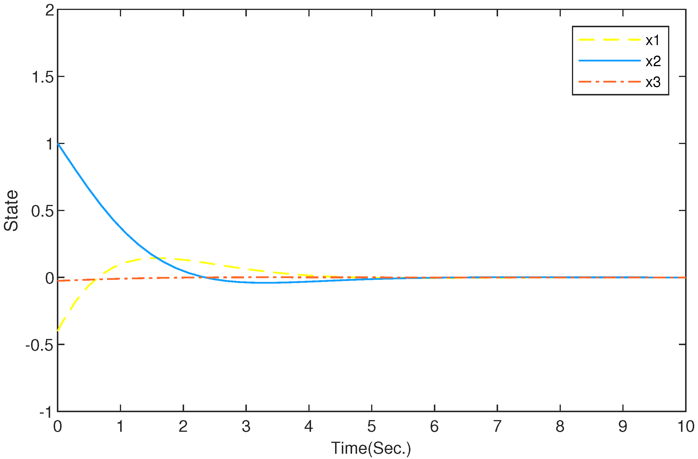
Example 3.
Consider system (1) with fractional order and , respectively, and
From Definition 1, we easily find that system (1) is not admissible because it does not meet the third property in Definition 1, i.e., system (1) is not stable. Therefore, we solve Equations (4) and (28) through Theorem 3 (Appendix A), and obtain the following feasible solutions:
Using the method of obtaining L and R in Example 2, we have
Through Theorem 4, we solve Equations (21) and (30) to obtain feasible solutions with fewer solving variables:
According to the data provided by the above simulation, we describe the state response when α takes different values through Figure 1, Figure 2 and Figure 3. Obviously, although the original open-loop systems are not admissible, the corresponding closed-loop systems are admissible under the influence of the control law (26) and reach stability in 50 , 5 , and 14 , respectively.
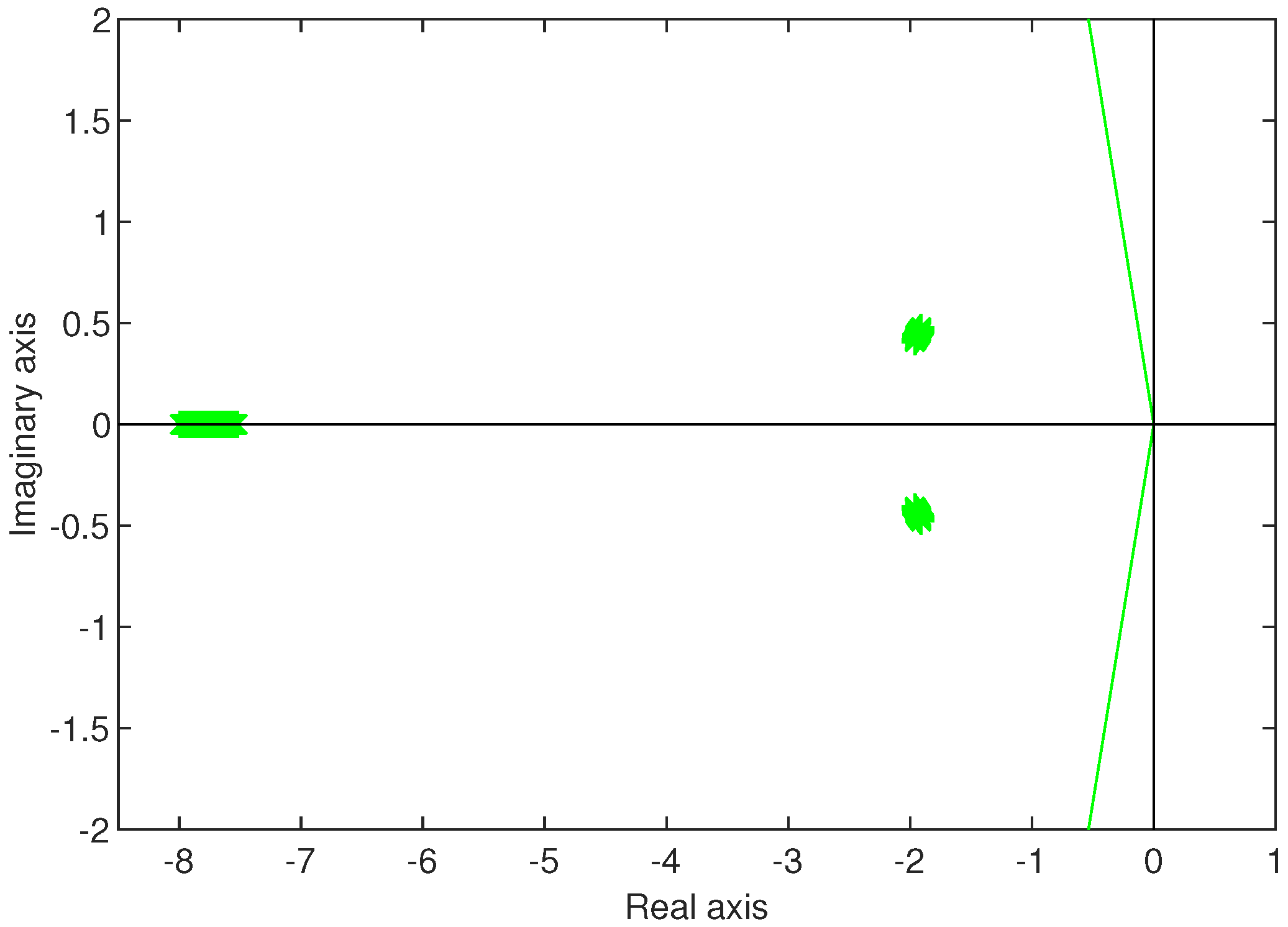
Example 4.
Using the method of obtaining L and R in Example 2, we have
We easily prove that although system (39) is regular and impulse-free, it is unstable. That is, system (39) is not admissible. Thanks to Theorem 8, we solve Equations (21), (23) and (40), and obtain the following feasible solutions:
It is seen from Figure 4 and Figure 5 that when α is and , respectively, the eigenvalues of the closed-loop systems are in the stability region. That is, although the original open-loop systems are not admissible, their corresponding closed-loop systems are admissible under the influence of the control law (41).
5. Conclusions
In this paper, the different necessary and sufficient conditions for the admissibility and quadratic admissibility of a class of singular FOSs with fractional order in the interval were investigated. In order to analyze the admissibility of singular systems, we proposed the methods of LMIs. The state feedback controller was given to solve the problem of quadratic admissibility of norm-bounded uncertain systems with fractional order in the range without any separation. When and , singular FOSs were simplified into normal FOSs and singular IOSs, respectively. Therefore, these results extended the Lyapunov stability and quadratic admissibility theorem from normal IOSs to singular FOSs with fractional order of . In the future, we will further study the control for singular FOSs with order and the adaptive-sliding mode fault-tolerant control for interval type-2 fuzzy singular FOSs.
Author Contributions
Conceptualization, methodology, software, validation, Y.W., X.Z., P.S. and D.B.; formal analysis, X.Z. and D.B.; investigation, Y.W.; resources, X.Z. and D.B.; data curation, Y.W.; writing—original draft preparation, Y.W.; writing—review and editing, X.Z. and D.B.; visualization, Y.W. and D.B.; supervision, X.Z., P.S. and D.B.; project administration, X.Z.; funding acquisition, X.Z. All authors have read and agreed to the published version of the manuscript.
Funding
This work was supported by fundamental research funds for the central universities (N2224005-3) and national key research and development program topic (2020YFB1710003).
Data Availability Statement
Not applicable.
Conflicts of Interest
The authors declare no conflict of interest.
Appendix A
The partial LMI algorithm for solving matrices X, Q and Z with Theorem 3 is given below.
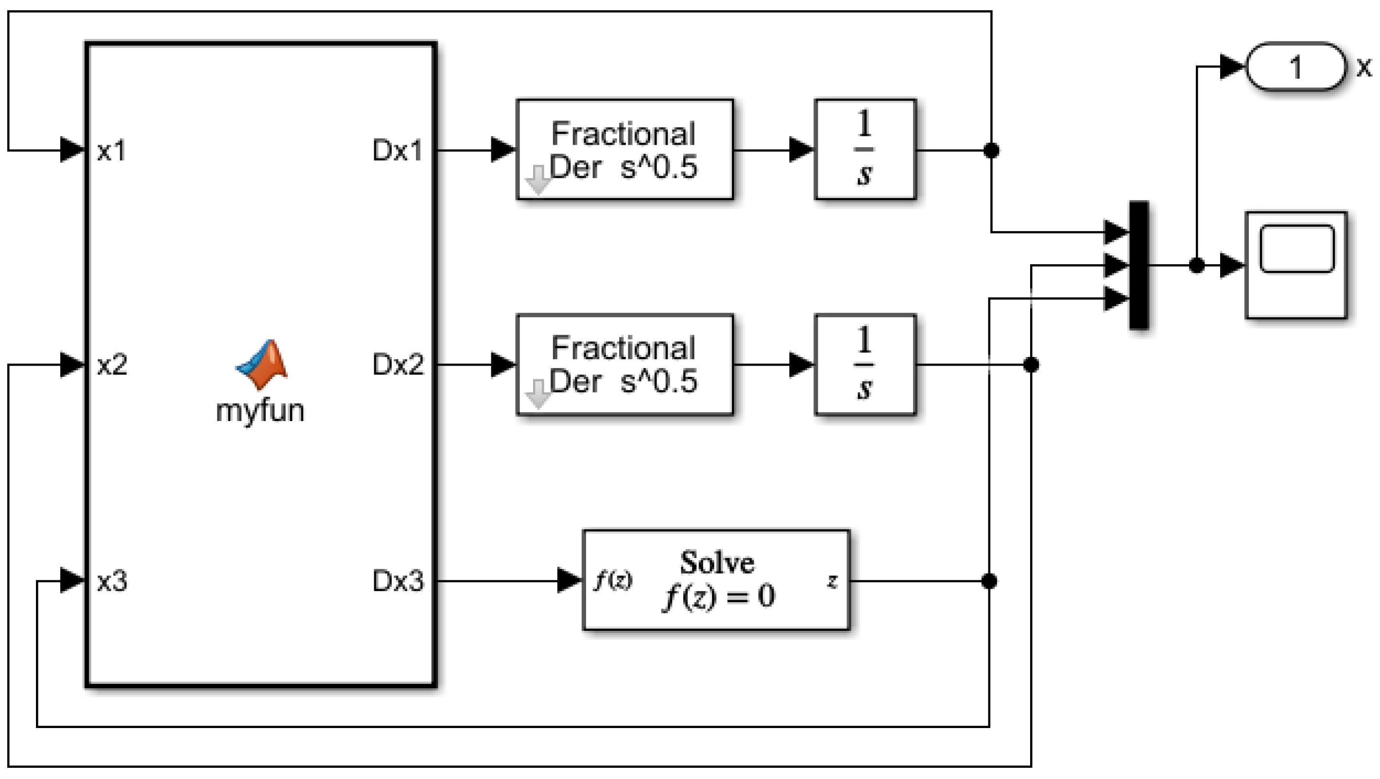
Figure A1 shows a singular FOS model. The module mainly contains the m-function, the fractional-order operator, and the integer-order integrator, the latter two combined into a fractional-order integrator. We adjusted the data in the m-function and integrator according to the simulation needs to get the required relevant data for the singular FOS.
| Algorithm 1: The partial LMI algorithm for solving matrices X, Q and Z with Theorem 3 |
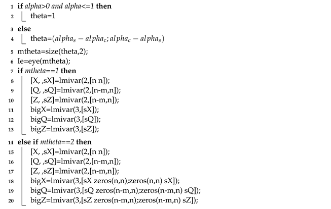 |
Figure A1.
Singular FOS model.
References
- Tavazoei, M.; Haeri, M. Rational approximations in the simulation and implementation of fractional-order dynamics: A descriptor system approach. Automatica 2010, 46, 94–100. [Google Scholar] [CrossRef]
- Aguila-Camacho, N.; Duarte-Mermoud, M.; Gallegos, J. Lyapunov functions for fractional order systems. Commun. Nonlin. Sci. Numer. Simul. 2014, 19, 2951–2957. [Google Scholar] [CrossRef]
- Zhang, J.X.; Wang, Q.G.; Ding, W. Global output-feedback prescribed performance control of nonlinear systems with unknown virtual control coefficients. IEEE Trans. Automat. Contr. 2021, 99, 1. [Google Scholar] [CrossRef]
- Zhang, J.X.; Yang, G.H. Fault-tolerant output-constrained control of unknown Euler-Lagrange systems with prescribed tracking accuracy. Automatica 2020, 111, 108606. [Google Scholar] [CrossRef]
- Zhang, X.F.; Huang, W.K.; Wang, Q.G. Robust H∞ adaptive sliding mode fault tolerant control for T-S fuzzy fractional order systems with mismatched disturbances. IEEE Trans. Circuits Syst. I Reg. Pap. 2021, 68, 1297–1307. [Google Scholar] [CrossRef]
- Zhan, T.; Liu, X.; Ma, S. A new singular system approach to output feedback sliding mode control for fractional order nonlinear systems. J. Franklin Inst. 2018, 355, 6746–6762. [Google Scholar] [CrossRef]
- Ahn, H.; Chen, Y. Necessary and sufficient stability condition of fractional-order interval linear systems. Automatica 2008, 44, 2985–2988. [Google Scholar] [CrossRef]
- N’Doye, I.; Darouach, M.; Zasadzinski, M.; Radhy, N. Robust stabilization of uncertain descriptor fractional-order systems. Automatica 2013, 49, 1907–1913. [Google Scholar] [CrossRef]
- Khargonekar, P.; Petersen, I.; Zhou, K. Robust stabilization of uncertain linear systems: Quadratic stabilizability and H∞ control theory. IEEE Trans. Automat. Contr. 1990, 35, 356–361. [Google Scholar] [CrossRef]
- Kebria, P.M.; Khosravi, A.; Nahavandi, S.; Shi, P.; Alizadehsani, R. Robust adaptive control scheme for teleoperation systems with delay and uncertainties. IEEE Trans. Cybern. 2020, 50, 3243–3253. [Google Scholar] [CrossRef]
- Li, Y.; Chen, Y.; Podlubny, I. Mittag–Leffler stability of fractional order nonlinear dynamic systems. Automatica 2009, 45, 1965–1969. [Google Scholar] [CrossRef]
- Yu, J.; Hu, H.; Zhou, S.; Lin, X. Generalized Mittag-Leffler stability of multi-variables fractional order nonlinear systems. Automatica 2013, 49, 1798–1803. [Google Scholar] [CrossRef]
- Lu, J.G.; Chen, Y.Q. Robust stability and stabilization of fractional order interval systems with the fractional order α: The 0 < α < 1 case. IEEE Trans. Automat. Contr. 2010, 55, 152–158. [Google Scholar]
- Semary, M.; Radwan, A.; Hassan, H. Fundamentals of fractional-order LTI circuits and systems: Number of poles, stability, time and frequency responses. Int. J. Circuit Theory Appl. 2016, 44, 2114–2133. [Google Scholar] [CrossRef]
- Alagoz, B. Hurwitz stability analysis of fractional order LTI systems according to principal characteristic equations. ISA Trans. 2017, 70, 7–15. [Google Scholar] [CrossRef] [PubMed]
- Kharade, J.; Kucche, K. On the impulsive implicit Ψ-Hilfer fractional differential equations with delay. Math. Methods Appl. Sci. 2020, 43, 1938–1952. [Google Scholar] [CrossRef] [Green Version]
- Wang, J.; Zhou, Y. Mittag-Leffler-Ulam stabilities of fractional evolution equations. Appl. Math. Lett. 2012, 25, 723–728. [Google Scholar] [CrossRef] [Green Version]
- Abu-Shady, M.; Kaabar, M. A generalized definition of the fractional derivative with applications. Math. Probl. Eng. 2021, 2021, 1–9. [Google Scholar] [CrossRef]
- Abu-Shady, M.; Kaabar, M. A novel computational tool for the fractional-order special functions arising from modeling scientific phenomena via Abu-Shady-Kaabar fractional derivative. Comput. Math. Methods Med. 2022, 2022, 2138775. [Google Scholar] [CrossRef]
- Ibrir, S.; Bettayeb, M. New sufficient conditions for observer-based control of fractional-order uncertain systems. Automatica 2015, 59, 216–223. [Google Scholar] [CrossRef]
- Farges, C.; Moze, M.; Sabatier, J. Pseudo-state feedback stabilization of commensurate fractional order systems. Automatica 2010, 46, 1730–1734. [Google Scholar] [CrossRef]
- Zhang, X.F.; Lin, C.; Chen, Y.Q.; Boutat, D. A unified framework of stability theorems for LTI fractional order systems with 0 < α < 2. IEEE Trans. Circuits Syst. II Express Briefs 2020, 67, 3237–3241. [Google Scholar]
- Xu, S.Y.; Lam, J. Robust Control and Filtering of Singular Systems; Springer: Berlin, Germany, 2006; pp. 31–44. [Google Scholar]
- Lin, C.; Wang, J.L.; Yang, G.H.; Lam, J. Robust stabilization via state feedback for descriptor systems with uncertainties in the derivative matrix. Int. J. Control 1999, 32, 3319–3324. [Google Scholar] [CrossRef]
- Xu, S.Y.; Van Dooren, P.; Stefan, R.; Lam, J. Robust stability and stabilization for singular systems with state delay and parameter uncertainty. IEEE Trans. Automat. Contr. 2002, 47, 1122–1128. [Google Scholar]
- Yu, Y.; Jiao, Z.; Sun, C.Y. Sufficient and necessary condition of admissibility for fractional-order singular system. Acta Autom. Sin. 2013, 39, 2160–2164. [Google Scholar] [CrossRef]
- Wei, Y.H.; Tse, P.; Yao, Z.; Wang, Y. The output feedback control synthesis for a class of singular fractional order systems. ISA Trans. 2017, 69, 1–9. [Google Scholar] [CrossRef]
- Zhang, X.F.; Chen, Y.Q. Admissibility and robust stabilization of continuous linear singular fractional order systems with the fractional order α: The 0 < α < 1 case. ISA Trans. 2018, 82, 42–50. [Google Scholar]
- Marir, S.; Chadli, M.; Bouagada, D. New admissibility conditions for singular linear continuous-time fractional-order systems. J. Franklin Inst. 2017, 354, 752–766. [Google Scholar] [CrossRef]
- Zhang, Q.H.; Lu, J.G.; Ma, Y.D.; Chen, Y.Q. Time domain solution analysis and novel admissibility conditions of singular fractional-order systems. IEEE Trans. Circuits Syst. I Regul. Pap. 2021, 68, 842–855. [Google Scholar] [CrossRef]
- Zhang, Q.H.; Lu, J.G. Necessary and sufficient conditions for extended strictly positive realness of singular fractional-order systems. IEEE Trans. Circuits Syst. II Express Briefs 2021, 68, 1997–2001. [Google Scholar] [CrossRef]
- Ji, Y.; Qiu, J. Stabilization of fractional-order singular uncertain systems. ISA Trans. 2015, 56, 53–64. [Google Scholar] [CrossRef] [PubMed]
- Marir, S.; Chadli, M. Robust admissibility and stabilization of uncertain singular fractional-order linear time-invariant systems. IEEE/CAA J. Autom. Sin. 2019, 6, 685–692. [Google Scholar] [CrossRef]
- Li, R.C.; Zhang, X.F. Adaptive sliding mode observer design for a class of T-S fuzzy descriptor fractional order systems. IEEE Trans. Fuzzy Syst. 2020, 28, 1951–1959. [Google Scholar] [CrossRef]
- Zhang, X.F.; Zhao, Z.L. Normalization and stabilization for rectangular singular fractional order T-S fuzzy systems. Fuzzy Sets Syst. 2020, 38, 140–153. [Google Scholar] [CrossRef]
- Yin, C.; Zhong, S.; Huang, X.; Cheng, Y. Robust stability analysis of fractional-order uncertain singular nonlinear system with external disturbance. Appl. Math. Comput. 2015, 269, 351–362. [Google Scholar] [CrossRef]
- Li, Y.; Wei, Y.; Chen, Y.; Wang, Y. A universal framework of the generalized Kalman–Yakubovich–Popov lemma for singular fractional-order systems. IEEE Trans. Syst. Man Cybern. Syst. 2021, 51, 5209–5217. [Google Scholar] [CrossRef]
- Marir, S.; Chadli, M.; Basin, M. Bounded real lemma for singular linear continuous-time fractional-order systems. Automatica 2022, 135, 109962. [Google Scholar] [CrossRef]
- Wei, Y.; Wang, J.; Liu, T.; Wang, Y. Sufficient and necessary conditions for stabilizing singular fractional order systems with partially measurable state. J. Franklin Inst. 2019, 356, 1975–1990. [Google Scholar] [CrossRef] [Green Version]
- Zhang, X.F.; Huang, W.K. Adaptive neural network sliding mode control for nonlinear singular fractional order systems with mismatched uncertainties. Fractal Fract. 2020, 4, 50. [Google Scholar] [CrossRef]
- Zhang, J.X.; Yang, G.H. Low-complexity tracking control of strict-feedback systems with unknown control directions. IEEE Trans. Automat. Contr. 2019, 64, 5175–5182. [Google Scholar] [CrossRef]
- Wang, Y.; He, P.; Shi, P.; Zhang, H. Fault detection for systems with model uncertainty and disturbance via coprime factorization and gap metric. IEEE Trans. Cybern. 2022, 52, 7765–7775. [Google Scholar] [CrossRef] [PubMed]
- Zhang, J.X.; Yang, G.H. Robust adaptive fault-tolerant control for a class of unknown nonlinear systems. IEEE Trans. Ind. Electron. 2017, 64, 585–594. [Google Scholar] [CrossRef]
- Zhang, J.X.; Yang, G.H. Fuzzy adaptive output feedback control of uncertain nonlinear systems with prescribed performance. IEEE Trans. Cybern. 2018, 48, 1342–1354. [Google Scholar] [CrossRef] [PubMed]
Figure 1.
Time response of the closed-loop singular FOS with order .
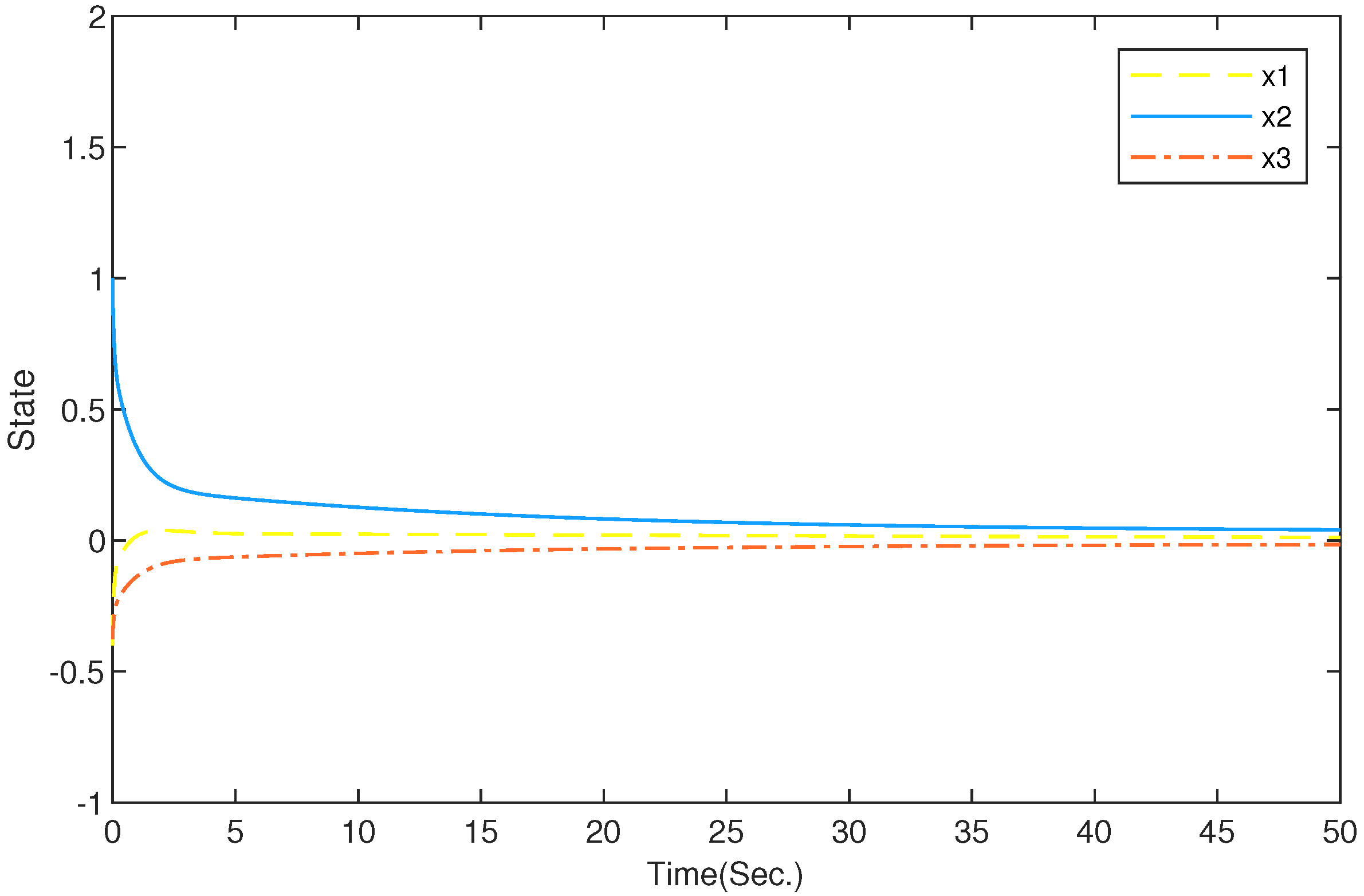
Figure 2.
Time response of the closed-loop singular FOS with order .

Figure 3.
Time response of the closed-loop singular FOS with order .
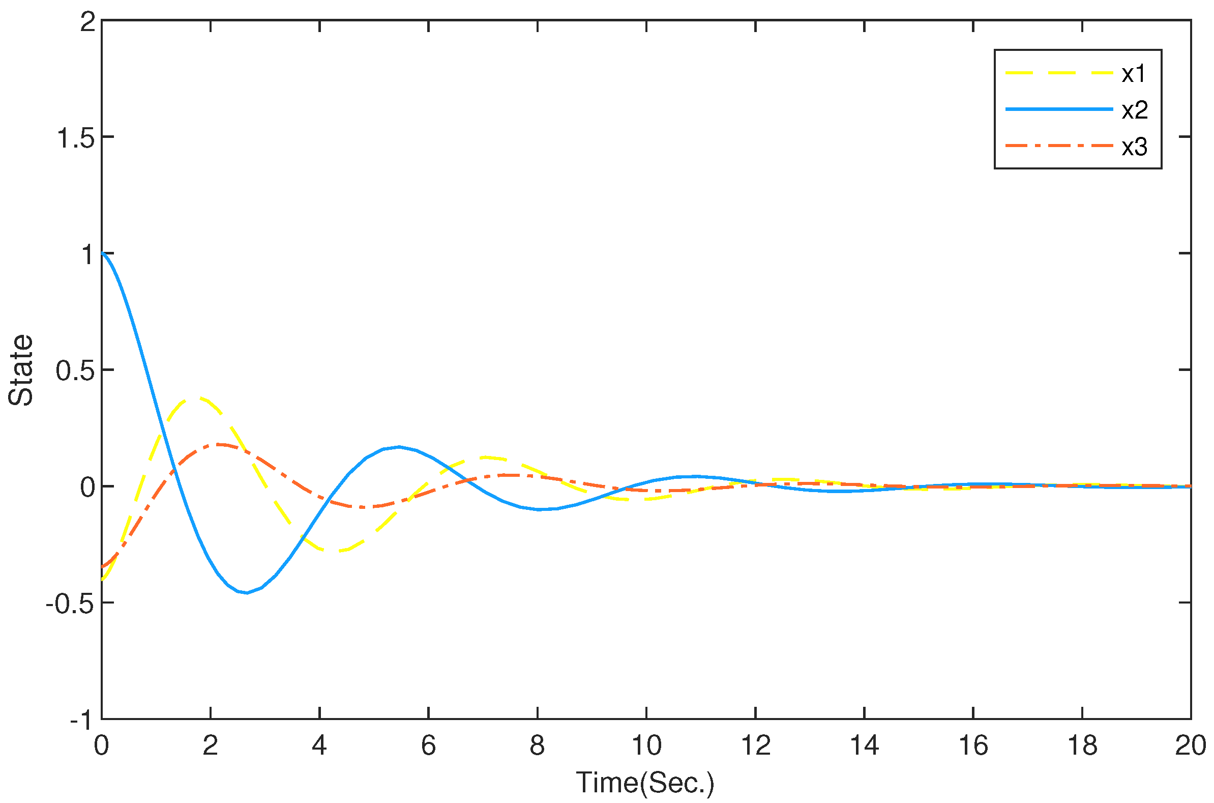
Figure 4.
Eigenvalue perturbation region of system with order .
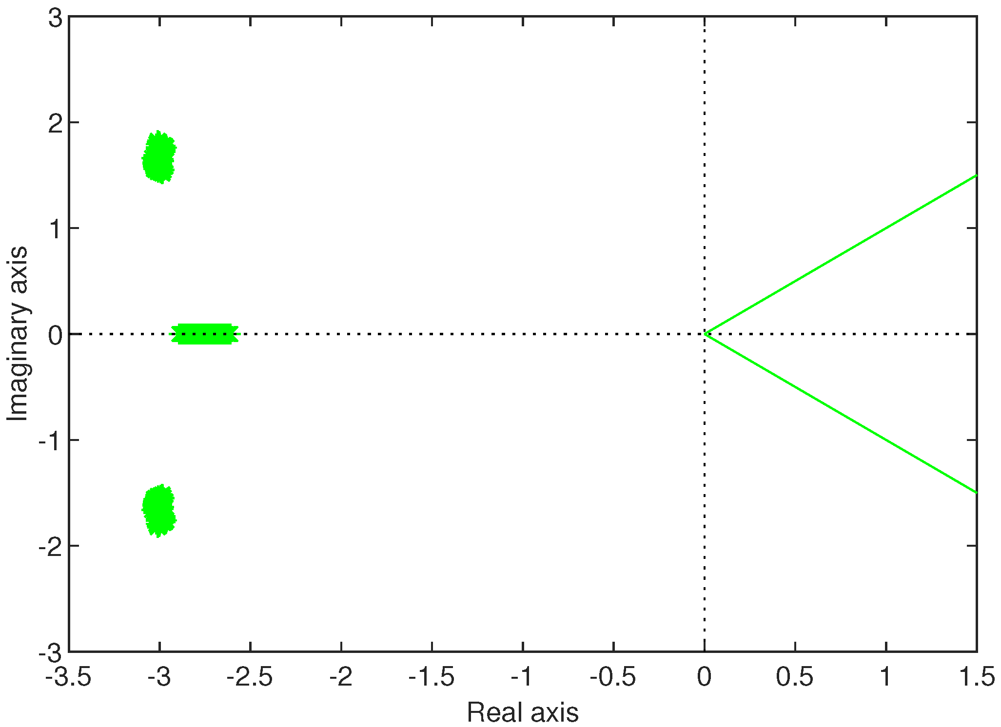
Figure 5.
Eigenvalue perturbation region of system with order .
Disclaimer/Publisher’s Note: The statements, opinions and data contained in all publications are solely those of the individual author(s) and contributor(s) and not of MDPI and/or the editor(s). MDPI and/or the editor(s) disclaim responsibility for any injury to people or property resulting from any ideas, methods, instructions or products referred to in the content. |
© 2022 by the authors. Licensee MDPI, Basel, Switzerland. This article is an open access article distributed under the terms and conditions of the Creative Commons Attribution (CC BY) license (https://creativecommons.org/licenses/by/4.0/).
Share and Cite
MDPI and ACS Style
Wang, Y.; Zhang, X.; Boutat, D.; Shi, P. Quadratic Admissibility for a Class of LTI Uncertain Singular Fractional-Order Systems with 0 < α < 2. Fractal Fract. 2023, 7, 1. https://doi.org/10.3390/fractalfract7010001
AMA Style
Wang Y, Zhang X, Boutat D, Shi P. Quadratic Admissibility for a Class of LTI Uncertain Singular Fractional-Order Systems with 0 < α < 2. Fractal and Fractional. 2023; 7(1):1. https://doi.org/10.3390/fractalfract7010001
Chicago/Turabian StyleWang, Yuying, Xuefeng Zhang, Driss Boutat, and Peng Shi. 2023. "Quadratic Admissibility for a Class of LTI Uncertain Singular Fractional-Order Systems with 0 < α < 2" Fractal and Fractional 7, no. 1: 1. https://doi.org/10.3390/fractalfract7010001