An Insight into the Impacts of Memory, Selling Price and Displayed Stock on a Retailer’s Decision in an Inventory Management Problem

Abstract

The present paper aims to demonstrate the combined impact of memory, selling price, and exhibited stock on a retailer’s decision to maximizing the profit. Exhibited stock endorses demand and low selling prices are also helpful for creating demand. The proposed mathematical model considers demand as a linear function of selling price and displayed inventory. This work utilized fractional calculus to design a memory-based decision-making environment. Following the analytical theory, an algorithm was designed, and by using the Mathematica software, we produced the numerical optimization results. Firstly, the work shows that memory negatively influences the retailer’s goal of maximum profit, which is the most important consequence of the numerical result. Secondly, raising the selling price will maximize the profit though the selling price, and demand will be negatively correlated. Finally, compared to the selling price, the influence of the visible stock is slightly lessened. The theoretical and numerical results ultimately imply that there can be no shortage and memory restrictions, leading to the highest average profit. The recommended approach may be used in retailing scenarios for small start-up businesses when a warehouse is required for continuous supply, but a showroom is not a top concern.

1. Introduction

Demand forecasting and optimal lot-size scheduling are essential issues for a retailing organization. Retailers have aimed to follow consumer demand since the beginning. More specifically, the earlier tendency in research on the best course of action for retail businesses focused only on predicting customer demand. The simple principle was “buy one, sell one.” Companies quickly realized, however, that employing more effective retailing strategies, including batch scheduling, could be more standardized, scalable, and could optimize profit. Batch scheduling organizes retailing operations so that final product components are created in groups, sometimes called batches, rather than in a continuous stream. Economic order quantity and production quantity modeling are two popular approaches in decision-making related to searching for optimal stock to maximize profit. Demand is an essential keyword in this context. Early literature on EOQ(Economic Order Quantity) models used constant demands [1,2,3,4,5].On the contrary, several variables may influence the market demand for a product. The items’ price, quality and reliability significantly impact demand. The theory of EOQ models has been evaluated by adding more reliable components in constructing the demand functions. The product’s price is such an important component that it has much control over the market demand for an item. Generally, the low-price value of commodities can act as a booster to create additional demand in the market. On the other hand, the stock in a retail organization’s showroom might provide a favorable impression of the organization’s capacity to meet client demand. Additionally, the involvement of human interactions makes the whole retailing scenario memory-motivated. The retail procedure cannot be a discrete incident. Both the retailer and the customer must have some experience due to their communication in the past. The present bargain may be influenced by the retailer’s and the customer’s prior experiences. Both the retailer and the customer can optimize their goal by utilizing their earned experience. The earned experience is termed memory, and the experience’s impact on decision-making phenomena is said to be the memory effect. We consider fractional calculus to capture the possibility of the iterative nature of the dynamics of an EOQ model. This paper considers an EOQ model, assuming that the demand is a function of price and stock, allowing shortages in the lot cycle. Furthermore, the model is supposed to be memory-sensitive, and a fractional differential equation is taken to be a working tool to describe it. This model is distinctive because it estimates the simultaneous effect of pricing, displayed stock, scarcity, and memory on merchants’ judgments, even though many researchers have previously conducted some experiments that are similar to this one. The demand is price-and stock-dependent, and the order quantity model is supposed to go through the fully backlogged shortage in a memory-based decision-making scenario. The subsections of the present section will summarize the existing literature, research gaps, and motivations related to the formulation of the proposed problem of this paper.

1.1. Basic Idea of Fractional Calculus and Memory Effect

Fractional calculus was initially used around three centuries ago, but due to the lack of a solution technique and a physical interpretation, its evolution in the first two centuries was relatively slow. The fundamental definition of the fractional derivative has changed since its inception (see [6,7]). Although the basic notion is evolving, the researchers have not provided any physical insight regarding the fractional derivative. It can recall the consequences of the inputs from the past to predict the present value of the output, which is one of the most valuable physical interpretations later discovered (see Saeedian et al. [8]; Tarasov and Tarasova, [9]). Furthermore, fractional calculus has non-Markovian characteristics. In this case, the memory index is represented by the fractional-order derivative and integration. As a result, fractional calculus is a suitable method for incorporating the memory effect into mathematical models of economic [10,11] and biological [8] problems. In light of this, one might say that it is the proper mathematical way to comprehend the true nature. In the past 30 years, fractional calculus has gained interest in several mathematics topics [12,13,14,15,16]. Agarwal et al. [17] contributed a pioneering theory of fractional calculus under uncertainty. Salahshour et al. [18] solved a fractional differential equation in fuzzy environment using the theory of fuzzy Laplace transformation. To account for memory effects on the inventory system, why must we need afractional-order derivative? First-order ODEs regulate traditional inventory models with integer-order derivatives. However, derivatives of integer orders for a differentiable time function are defined only in an infinitely small neighborhood of the measured point of time. Due to its inability to describe the system’s memory impact, the traditional inventory model suffers from forgetfulness. Amnesia may be removed from any system using the fractional-order system [19]. The memory effect on the inventory system is something we want to consider while creating a fractional-order inventory model for the reasons mentioned above. The order of a fractional derivative determines how strong a memory is.

1.2. EOQ Models and Fractional Calculus

This subsection provides a brief review of the recent developments of the literature related to the economic order and production quantity models. The review process has been carried out based on the keywords: selling price, displayed stocks, deterioration, preservation, shortage, learning, memory, etc.

It is mentioned earlier in this section that demand is a very crucial component in a production–supply scenario. The initial demand pattern trend is considered a constant and deterministic one. However, market demand may depend on different features. The selling price of products is one such crucial issue that is impacting demand. Very often, it is seen that the high selling price of products hurts the demand. Sometimes retailers offer the customers small (discounted) selling priced items, creating huge sales of those items. Many inventory models predict that reduced pricing will result in greater demand. For an EOQ model with quantity discounts and price-dependent demand, Transchel and Minner [20] devised optimum solution methods while treating the linear price function as a particular case. They investigated various approaches, including adjusting the selling price while calculating the lot size concurrently. Sana [21] experimented with stochastic price-dependent demand with the fully backlogged shortage for a newsboy problem. In the case of shortage, an EOQ model with price-dependent demand was investigated by Pal et al. [22]. The notion of a time-varying holding cost and discount policy in the inventory model with price-dependent demand was implemented by Alfares and Ghaithan [23]. Das et al. [24] prescribed the utilization of preservation technology on an inventory model of deteriorating items, assuming price-dependent demand and partial backlogging. Rahman et al. [25] discussed an EOQ model with a price-dependent demand rate in uncertain phenomena, considering all the decision parameters as interval numbers.

Another critical issue is the product’s supply in the inventory cycle. Unsellable items caused by arbitrary vast amounts of stock may result in the retailer’s final loss. However, the displayed store in a showroom may help earn customer’s interests and stock can be incorporated in the list of essential components controlling the demand function. Inventory models that base demand on item availability or stock levels are popular. Min and Zhou [26] studied an inventory model for depreciating commodities, considering a demand that depends on the stock level, some backlogs, and a maximum inventory level cap. Yang et al. [27] developed another inventory model that incorporates stock-dependent demand for depreciating items, allows for some backlog, and accounts for inflation. An inventory model with a stock-dependent demand rate and inflation was given by Singh et al. [28] for goods sold from primary and secondary stores under single management. Bhunia and Shaikh [29] considered the effects of various marketing tactics, including price and advertising, and the visible inventory level on the system’s demand rate. Lee and Dye [30] created an EOQ model with a partial backlog, stock-dependent demand, and a regulated deterioration rate; the model chooses the best ordering and deterioration management strategies to maximize the overall profit. Bhunia et al. [31] analyzed different retailing scenarios of price-breaking unit discount policies and displayed stock-dependent demand. Shaikh et al. [32] considered inflation for two warehouses with an inventory problem of deteriorating items with stock-dependent demand. They developed an uncertain decision-making policy incorporating interval valued costs.

The collective impact of price and stock on market demand was investigated by many researchers over the last two decades. Panda et al. [33] used the genetic algorithm to optimize a deteriorating inventory problem, assuming that the demand is a function of stock and price. Dye and Hsieh [34] studied a partially backlogged EOQ model with stock and price-dependent dependencies and customer waiting time depending on shortage. The optimization was carried out using particle swarm optimization (PSO). Sana [35] studied a deteriorating inventory model of stock and selling price-controlled demand and explored the fact that extensive uncontrolled stock negatively impacts the market for the product. Several more investigations [36,37,38,39] had been carried out in this direction. Shaikh et al. [40] developed an inventory model that considers demand as a function of stock and price, allows shortage to be fully backlogged, and uses PSO to optimize the problem. Mashud et al. [41] extended this work for the case of partial back-ordering. Again, Shaikh et al. [42] established a study on an inventory model where they considered the demand to be stock- and price-dependent, holding cost to be time-dependent, shortage to be fully back-ordered and customer’s waiting time to be dependent. Additionally, they allowed the deterioration of items and discount policy as presumptions. Khan et al. [43] incorporated discount opportunities for the retailer through partial and fully advanced payments in an order quantity model of deteriorating goods with price- and stock-dependent demand and shortage. Rahaman et al. [44] discussed a fuzzy economic production quantity model of decaying items, considering demand as a function of price and stock and production rate as a function of stock. They used the fuzzy differential equation approach to solve the problem. Later, Rahaman et al. [45] included a preservation management strategy to discuss a fuzzy EPQ model with the same assumption.

Additionally, the entire retailing setting may be memory-motivated due to interpersonal interactions. In this context, physical interpretations of fractional calculus are given to carry the memory of dynamical systems to the next level, with the iterated kernels involved in its several definitions in mathematical modeling. A comparison of contributions from recent publications on EOQ models employing fractional calculus is shown in

Table 1. Comparison among the contributions of recent publications related to the proposed fractional inventory model.

Authors	Year	Demand Function	Methodology
Das and Roy [46]	2014	Constant demand	Primal geometric programming for optimization
Das and Roy [47]	2015	Lineartime-dependent demand	Primal geometric programming for optimization
Pakhira et al. [48]	2018	Linear time-dependent demand	Primal geometric programming for optimization
Pakhira et al. [49]	2018	Linear time-dependent demand	Primal geometric programming for optimization
Pakhira et al. [50]	2019	Quadratic time-dependent demand	Primal geometric programming for optimization
Pakhira et al. [51]	2019	Linear time-dependent fuzzy demand	Primal geometric programming for optimization and signed distance method for defuzzification
Pakhira et al. [52]	2020	Time and order of fractional derivative dependent demand	Primal geometric programming for optimization
Pakhira et al. [53]	2020	Time-dependent Mittag–Leffler function distributed demand	Primal geometric programming for optimization
Rahaman et al. [54]	2021	Time-dependent decreasing fuzzy demand	Fractional differential equation and dense fuzzy environment optimization
Rahaman et al. [55]	2021	Fuzzy price dependent demand	Fuzzy fractional differential equation and lock fuzzy dense environment of optimization
Rahaman et al. [56]	2022	Fuzzy constant demand	Fuzzy fractional differential equation and trapezoidal fuzzy environment of optimization
This paper		Price and displayed stock dependent demand	Mathematical analysis using fractional calculus and numerical optimization through a proposed algorithm by using Mathematica software(Company Name: Wolfram Research, Inc. Headquarter: Champaign, IL, United States)

. This table compares the literature based on various demand functions and solution techniques.

1.3. Motivation of the Work

The following are several gaps identified in recent work on lot-size modeling and their applications for the field of fractional calculus applications. The proposed work is intended to fill these gaps below:

• A massive volume of literature exists that is related to the EOQ/EPQ(Economic Production Quantity) model. However, there is no such significant number of papers to date dealing with the impact of memory on the decision-making procedure.
• There are enough reasons to consider the EOQ/EPQ models in memory-sensitive situations. In reality, a decision-making phenomenon involving human’s association cannot be memory-free.
• To date, most of the memory-sensitive model discussed in the light of fractional calculus is developed on the assumptions of constant demand, price, or time-dependent demand. Furthermore, they are inferior in numbers compared to the whole literature on the theories of EOQ and EPQ models.
• Consequently, there are motives for including the memory sense in lot-size modelling, but the literature is still in its infancy. The analysis of fractional calculus is complicated, which might be the cause.

1.4. Novelties of the Work

An EOQ model with selling price and stock-dependent demand rate under a fully backlogged shortage has been taken in a memory-sensitive situation to fill the aforementioned gaps. The significant contributions of this paper are as follows:

• This paper manifests the collective impact of pricing, displayed stock, shortage, and memory on retailers’ decisions. This paper uses demand as a function of selling price and displayed stock to formulate the model. The model is discussed for both the cases of shortage and without shortage. It also incorporates memory sense in theory utilizing fractional calculus tools. Several earlier studies addressed the mentioned features separately. But, no literature discussed the impacts simultaneously.
• An algorithm for solving the optimization model that corresponds to the proposed EOQ is created for quantitative analysis by using the Mathematica software.
• The given mathematical model provides significant management insight into a business phenomenon. This concept can be used for freshly established retail businesses when the showroom is still being constructed. The proposedmodel in this research might be applied to the small-scale retailing of bakeries and poultry slaughtering.

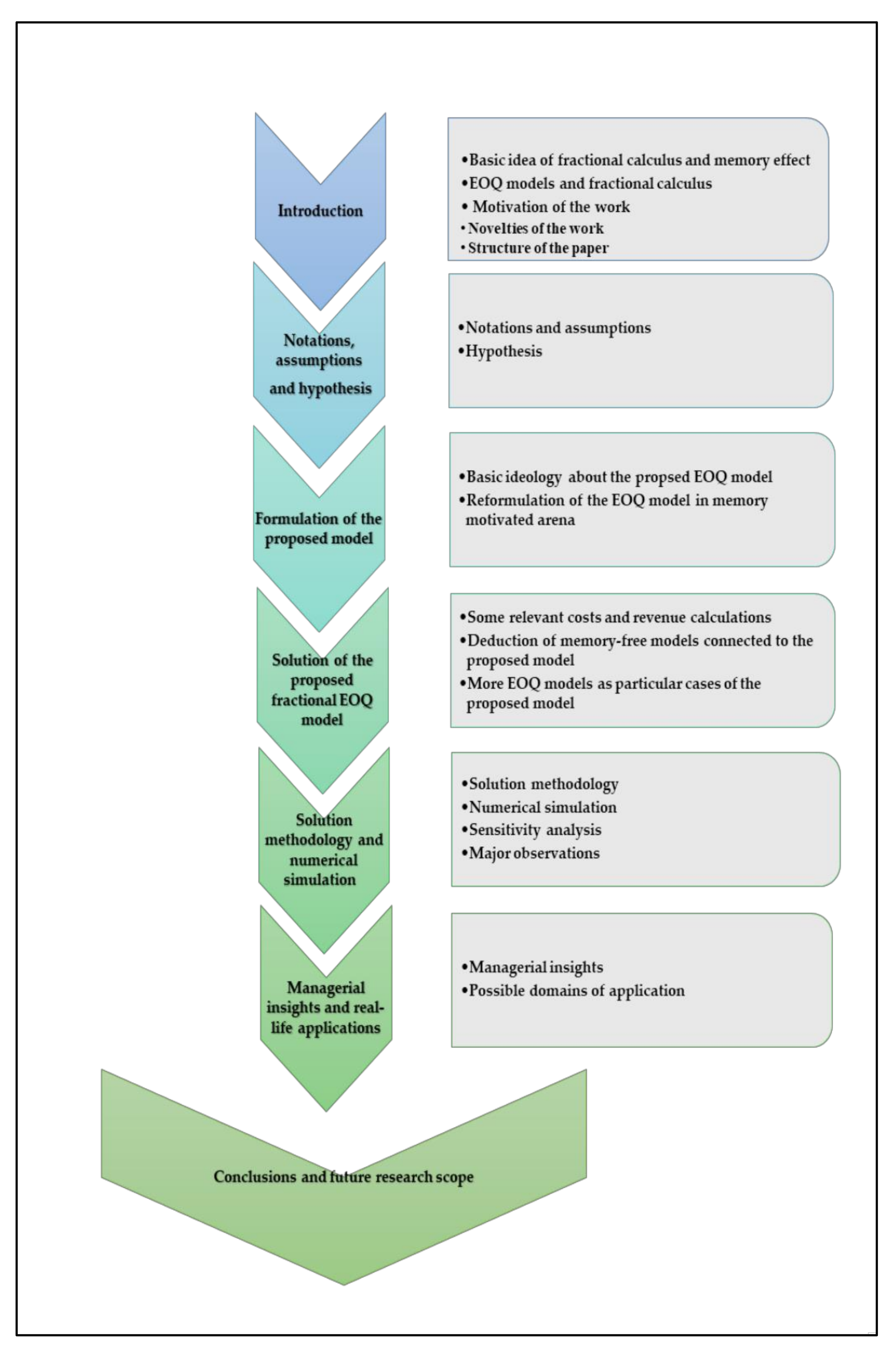
1.5. Structure of the Paper

The rest of the paper is also organized with different sections and subsections. The whole paper contains seven sections and several subsections which are visually represented in Figure 1.

For the above Figure 1, the box in the right of each section’s name contains the title of their subsections. “Conclusions and future scope” section contains no subsections.

2. Notations, Assumptions and Hypothesis

This paper tries to formulate a more realistic model in the sense of memory sensitivity. Here, the demand is considered a linear stock and price function. With more displayed stock in the showroom, the demand can be increased. According to the polar opposite of how much an item’s selling price is, the demand for that specific commodity in a developing country’s culture must rise or fall. Additionally, both the customers and the retailer have some memory of past consumption and dealing attitudes, respectively. The customers are motivated by the experience with the retailers’ dealing behavior and the quality of the products they used earlier. On the counterpart, the retailer gained knowledge from the previous demand pattern. Thus, the entire situation must be memory affected. This paper incorporates these real concerns into modeling the proposed problem.

2.1. Notations and Assumptions

Several notations are used to describe the EOQ model.

Table 2. Symbols and notations with their units and meanings which are representing the objective functions, decision variables, different costs and revenues and coefficients in this paper.

Notations	Units	Descriptions
$h_c$	USD	Holding cost per unit stock
$S_{up}$	USD	Setup cost as initial investment for basic infrastructure
$s_c$	USD	Shortage cost as penalty per unit shortage
$p$	USD	Selling price per unit sold items
$D$	Unit	Demand rate which is a linear function of selling price and displayed stock
$T$	Month	Complete lot cycle which includes both of the retailing and shortage phase (a decision variable)
$T_1$	Month	Active retailing cycle (a decision variable)
$Q$	Unit	Optimal lot size for a retailing cycle (a decision variable)
$S_1$	Unit	Size of inventories at the beginning of a lot cycle (a decision variable)
$q\left(t\right)$	Unit	$\mathrm{Stock}\mathrm{as}\mathrm{a}\mathrm{function}\mathrm{of}\mathrm{time}t$
$s\left(t\right)$	Unit	$\mathrm{Shortage}\mathrm{as}\mathrm{a}\mathrm{function}\mathrm{of}\mathrm{time}t$
$\alpha$	Unit	Order of fractional derivative which is called differential memory index
$\beta$	Unit	Order of fractional integral which is called integral memory index
$a$	Unit	Demand potential which is a positive constant
$b$	Unit	Proportional constant for the relation between demand and selling price
C	Unit	Proportional constant for the relation between demand and displayed
$TA{P}_{\alpha ,\beta }$	USD	Total average profit for the memory-motivated model (objective function)
$TAP$	USD	Total average profit for the memory-free model (objective function)

lists the notations used in this article, their units, and their meanings.

2.2. Hypothesis

The model is framed on the below mentioned hypothesis:

(i)

Demand is linear function of selling price and displayed stock., i.e., $D\left(p,q\left(t\right)\right)=\{\begin{array}{c}a-bp+cq\left(t\right), where 0\le t\le T_1\\ a-bp, where T_1\le t\le T,\end{array}$ where $a,b,c$ are positive constants and $p$ is the selling price of the product.

(ii)

Shortage is allowed and completely backlogged.

(iii)

Replenishment rate is spontaneous and lead time is zero.

(iv)

Lot size and time horizon are finite.

(v)

The retailing phenomenon is memory-motivated.

Remark1.If one looks at Table 1 and considers the presumptions stated in Section 2.2, it is clear that the contribution is unique compared to earlier works. Research on fractional calculus and inventory management is not new. Still, it is new from the standpoint of considering the assumption mentioned above while using fractional calculus to solve the inventory management problem.

Remark 2. Looking closely, we can observe that demand in some inventory management situations is a non-linear stock and selling price function. In contrast, demand depends linearly on stock and selling prices in other cases. This article explores a specific inventory issue where demand is linearly correlated with stocks and selling prices. Future studies may consider the demand function’s logistic reliance on the stores [57]. In such a situation where memory is a factor in decision-making, the fractional-order logistic differential equation [58] may contribute to the inventory model.

3. Formulation of Proposed Model

Here, the establishment of the proposed model mathematically on the earlier mentioned assumptions is described in detail. The present section is organized with two subsections representing the formulation of the model and reformulation of the model in the fractional arena.

3.1. Basic Ideology about the Proposed EOQ Model

The lot cycle is started with the initial stock level $S_1$.The stock level decreases uniformly by adjusting demand during the whole inventory run period ($0\le t\le T_1$). At time $t=T_1$, the stock level becomes zero and the inventory run phase is stopped. The shortage phase ($T_1\le t\le T$) starts with the initial shortage amount zero unit at $t=T_1$. For unfulfilled demand during this time, the shortage level gradually increases. The overall inventory cycle is stopped at $t=T$ with its highest level of shortage $Q-S_1$.

Traditionally, the memory-free dynamical system of stock management can be described by the following differential equation:

Inventory run phase $(0\le t\le T_1$): The differential equation representing gradual declination of the inventory level during the active inventory run phase is

$$\frac{dq\left(t\right)}{dt}=-D\left(p,q\left(t\right)\right).$$

(1)

The negative sign in Equation (1) represents the negative proportionality of the stock growth $\frac{dq\left(t\right)}{dt}$ to the price and stock-dependent demand rate $D\left(p,q\left(t\right)\right)$.

Shortage phase $(T_1\le t\le T$): The differential equation representing the gradual ascending nature of the shortage level is

$$\frac{ds\left(t\right)}{dt}=D\left(p\right).$$

(2)

At the beginning of the inventory run period, the initial inventory level is $S_1$ and it is completely diminished to 0 at the end of the active phase. The terminal conditions regarding the stocks in the active inventory run phase are given by

$$\{\begin{array}{c}q\left(0\right)=S_1,\\ q\left(T_1\right)=0.\end{array}$$

(3)

There is no shortage when the active inventory phase is just ended. Therefore, the shortage level is zero at the very early stage $t=T_1$ of the shortage phase. Then, the highest level of shortage $Q-S_1$ is at the end of the decision cycle. The terminal conditions regarding the shortages are given by

$$\{\begin{array}{c}s\left(T_1\right)=0,\\ s\left(T\right)=Q-S_1.\end{array}$$

(4)

3.2. Reformulation of the EOQ Model in Memory-Motivated Arena

Suppose the system described in the earlier sub-section is considered memory-sensitive. In that case, the system can be reformulated in the light of the fractional calculus (see Appendix A) as follows:

Inventory run phase $(0\le t\le T_1$):

The sense of memory can be incorporated in the differential equation letting to be given in terms of differ-integral equation with iterated kernel. Thus, the differential Equation (1) representing the inventory run phase $(0\le t\le T_1$) takes the form

$$\frac{dq\left(t\right)}{dt}=-\underset{0}{\overset{t}{{\displaystyle \int }}}k\left(t,v\right)D\left(p,q\left(v\right)\right)dv.$$

(5)

In Equation (5), $k\left(t,v\right)$ is an iterative kernel that inherits memory from the previous deals. The standard delta function, $k\left(t,s\right)=\delta \left(t,s\right)$, represents a memory-less model in the classical differential equation. We take the kernel $k\left(t,v\right)=\frac{{\left(t-v\right)}^{\alpha -1}}{\Gamma (\alpha )}$ to receive the corresponding fractional analogue of Equation (1). Then, from Equation (5),

$$\begin{gathered} \frac{dq\left(t\right)}{dt}=-\underset{0}{\overset{t}{{\displaystyle \int }}}\frac{{\left(t-v\right)}^{\alpha -1}}{\Gamma (\alpha )}D\left(p,q\left(v\right)\right)dv, \\ i.e.,\frac{dq\left(t\right)}{dt}=-{}_{}{}^{RL}I{}_t^{\alpha -1}\left\{D\left(p,q\left(t\right)\right)\right\} \end{gathered}$$

(6)

$\mathrm{where}{}_{}{}^{RL}I{}_t^{\alpha -1}$ is the Riemann–Liouville integral operator of order $\alpha -1$ in Equation (6). Taking the Riemann–Liouville integral operator ${}_{}{}^{RL}I{}_t^{1-\alpha }$ of order $1-\alpha$ in both sides of Equation (6), it can be reduced to the following Caputo fractional differential equation of order $\alpha$

$${}_{}{}^{Cap}D{}_t^{\alpha }q\left(t\right)=-\left\{a-bp+cq\left(t\right)\right\}.$$

(7)

Shortage phase ($T_1\le t\le T$):

Similarly, the differential equation given by Equation (2) describing shortage phase ($T_1\le t\le T$) can be reduced to its fractional representative

$${}_{}{}^{Cap}D{}_t^{\alpha }s\left(t\right)=\left\{a-bp\right\}.$$

(8)

Thus, the Caputo fractional differential Equations (7) and (8), along with the Equations (3) and (4) represent the memory-sensitive inventory scenario with price and stock-dependent demand with a fully backlogged shortage. In the following subsection, we will solve Equations (7) and (8) with the tools of fractional calculus and construct a corresponding optimization problem.

4. Solution of the Proposed Fractional EOQ Model

In this section, we utilized primarily the Laplace transformation and inverse Laplace transformation to solve the Caputo fractional differential equation. Additionally, fractional integration is defined in first subsection to compute the relevant costs and revenue (see Appendix A). Additionally, the deduction of a simpler lot-size model from the proposed model has been discussed in subsequent subsections.

Inventory run phase ($0\le t\le T_1$):

Taking Laplace transformation on Equation (7) and using the initial condition $q\left(0\right)=S_1$ we receive the following expression:

$$\tilde{q}\left(u\right)=\frac{u^{\alpha }{S}_1}{u\left(u^{\alpha }+c\right)}-\frac{\left(a-bp\right)}{u\left(u^{\alpha }+c\right)}.$$

(9)

In Equation (9), $\tilde{q}\left(u\right)$ represents the Laplace transformation of the function $q\left(t\right)$.

Taking the inverse Laplace transformation of Equation (9),

$$q\left(t\right)=S_1{E}_{\alpha }\left(-c{t}^{\alpha }\right)-\frac{\left(a-bp\right)}{c}\left\{1-E_{\alpha }\left(-c{t}^{\alpha }\right)\right\}.$$

(10)

In Equation (10), $E_{\alpha }\left(-c{t}^{\alpha }\right)$ is the one parameter Mittag–Leffler function (see Appendix A) about $-c{t}^{\alpha }$. Using the terminal value of stock in the inventory run phase, $q\left(T_1\right)=0,$ the value of the initial stock level can be obtained explicitly as

$$S_1=\frac{\left(a-bp\right)}{c}\left[{\left\{E_{\alpha }\left(-c{T}_1{}^{\alpha }\right)\right\}}^{-1}-1\right].$$

(11)

The initial inventory level $S_1$ in memory-motivated phenomena is given by Equation (11).Then, using Equation (11), Equation (10) can be rewritten as

$$q\left(t\right)=\frac{\left(a-bp\right)}{c}\left[{\left\{E_{\alpha }\left(-c{T}_1{}^{\alpha }\right)\right\}}^{-1}{E}_{\alpha }\left(-c{t}^{\alpha }\right)-1\right]$$

(12)

$\mathrm{where}q\left(t\right)$ represents the stock function of time during inventory run phase in Equation (12).

Shortage phase ($T_1\le t\le T$):

Taking Laplace transformation on Equation (8) and using the initial condition $s\left(T_1\right)=0$ we receive the following expression:

$$\tilde{s}\left(u\right)=\frac{\left(a-bp\right)}{u^{\alpha +1}}.$$

(13)

In Equation (13), $\tilde{s}\left(u\right)$ represents the Laplace transformation of the function $s\left(t\right)$.

Taking the inverse Laplace transformation of Equation (13) we receive

$$s\left(t\right)=\frac{\left(a-bp\right){\left(t-T_1\right)}^{\alpha }}{\mathsf{\Gamma }\left(\alpha +1\right)}.$$

(14)

In Equation (14), $\Gamma \left(\alpha +1\right)$ is the traditional Gamma function about $\alpha +1$. Using the terminal value of shortage, $s\left(T\right)=Q-S_1$, the value of the total shortage can be estimated explicitly as

$$Q-S_1=\frac{\left(a-bp\right){\left(T-T_1\right)}^{\alpha }}{\mathsf{\Gamma }\left(\alpha +1\right)}.$$

(15)

Equation (15) represents the highest possible shortage in the decision cycle. From the Equations (11) and (15), the lot size of retailing phenomena is obtained as

$$Q=\left(a-bp\right)\left[\frac{{\left\{E_{\alpha }\left(-c{T}_1{}^{\alpha }\right)\right\}}^{-1}-1}{c}+\frac{{\left(T-T_1\right)}^{\alpha }}{\mathsf{\Gamma }\left(\alpha +1\right)}\right]$$

(16)

4.1. Some Relevant Costs and Revenue Calculations

(i)

Set up cost: This is onetime investment. It also includes the ordering cost and is taken as a constant $S_{up}$.

(ii)

Total holding cost: The holding cost per unit is $h_c$ and span of stock is $\left[0,T_1\right]$. Thus, the total holding cost $H{C}_{\alpha ,\beta }$ can be obtained by the following fractional integration of order $\beta$

$$\begin{array}{c}H{C}_{\alpha ,\beta }=\frac{h_c}{\mathsf{\Gamma }(\beta )}{{\displaystyle \int }}_0^{T_1}{\left(T_1-t\right)}^{\beta -1}q\left(t\right)dt\hfill \\ =\frac{h_c\left(a-bp\right)}{\mathsf{\Gamma }(\beta )c}{{\displaystyle \int }}_0^{T_1}{\left(T_1-t\right)}^{\beta -1}\left[{\left\{E_{\alpha }\left(-c{T}_1{}^{\alpha }\right)\right\}}^{-1}{E}_{\alpha }\left(-c{t}^{\alpha }\right)-1\right]dt\hfill \\ =\frac{h_c\left(a-bp\right)}{\mathsf{\Gamma }(\beta )c}\left[{\left\{E_{\alpha }\left(-c{T}_1{}^{\alpha }\right)\right\}}^{-1}{{\displaystyle \int }}_0^{T_1}{\left(T_1-t\right)}^{\beta -1}{E}_{\alpha }\left(-c{t}^{\alpha }\right)dt-\frac{T_1{}^{\beta }}{\beta }\right]\hfill \\ =\frac{h_c\left(a-bp\right)}{\mathsf{\Gamma }(\beta )c}\left[{\left\{E_{\alpha }\left(-c{T}_1{}^{\alpha }\right)\right\}}^{-1}{{\displaystyle \int }}_0^{T_1}{\left(T_1-t\right)}^{\beta -1}{\displaystyle {\displaystyle \sum }_{k=0}^{\infty }}\frac{{\left(-c{t}^{\alpha }\right)}^k}{\mathsf{\Gamma }\left(\alpha k+1\right)}dt-\frac{T_1{}^{\beta }}{\beta }\right]\hfill \\ =\frac{h_c\left(a-bp\right)}{\mathsf{\Gamma }(\beta )c}\left[{\left\{E_{\alpha }\left(-c{T}_1{}^{\alpha }\right)\right\}}^{-1}{\displaystyle {\displaystyle \sum }_{k=0}^{\infty }}\frac{{\left(-c\right)}^k}{\mathsf{\Gamma }\left(\alpha k+1\right)}{{\displaystyle \int }}_0^{T_1}{\left(T_1-t\right)}^{\beta -1}{t}^{\alpha k}dt-\frac{T_1{}^{\beta }}{\beta }\right]\hfill \\ =\frac{h_c\left(a-bp\right)}{\mathsf{\Gamma }(\beta )c}\left[{\left\{E_{\alpha }\left(-c{T}_1{}^{\alpha }\right)\right\}}^{-1}{\displaystyle {\displaystyle \sum }_{k=0}^{\infty }}\frac{{\left(-c\right)}^k{T}_1{}^{\alpha k+\beta }\mathsf{\Gamma }(\beta )}{\mathsf{\Gamma }\left(\alpha k+\beta +1\right)}-\frac{T_1{}^{\beta }}{\beta }\right]\hfill \\ =\frac{h_c\left(a-bp\right)T_1{}^{\beta }}{c}\left[{\left\{E_{\alpha }\left(-c{T}_1{}^{\alpha }\right)\right\}}^{-1}{E}_{\alpha ,\beta +1}\left(-c{T}_1{}^{\alpha }\right)-\frac{1}{\mathsf{\Gamma }\left(\beta +1\right)}\right]\hfill \end{array}$$

.

(iii)

Total shortage cost: The system is taken to be with shortage. Thus, there is a shortage cost per unit which is $s_c$ and the total shortage cost $S{C}_{\alpha ,\beta }$ on the time span $[T_1, T]$ as

$$\begin{array}{c}S{C}_{\alpha ,\beta }=\frac{s_c}{\mathsf{\Gamma }(\beta )}{{\displaystyle \int }}_{T_1}^T{\left(T-t\right)}^{\beta -1}s\left(t\right)dt\hfill \\ =\frac{s_c\left(a-bp\right)}{\mathsf{\Gamma }(\beta )\mathsf{\Gamma }\left(\alpha +1\right)}{{\displaystyle \int }}_{T_1}^T{\left(T-t\right)}^{\beta -1}{\left(t-T_1\right)}^{\alpha }dt\hfill \\ =\frac{s_c\left(a-bp\right){\left(T-T_1\right)}^{\alpha +\beta }\mathsf{{\rm B}}\left(\alpha +1,\beta \right)}{\mathsf{\Gamma }(\beta )\mathsf{\Gamma }\left(\alpha +1\right)}\hfill \\ =\frac{s_c\left(a-bp\right){\left(T-T_1\right)}^{\alpha +\beta }}{\mathsf{\Gamma }\left(\alpha +\beta +1\right)}.\hfill \end{array}$$

(iv)

Sales revenue: The selling price per unit is $p$ and span of stock is $\left[0,T_1\right]$. Thus, the tota sales revenue $S{R}_{\alpha ,\beta }$ can be

$$\begin{array}{c}S{R}_{\alpha ,\beta }=\frac{p}{\mathsf{\Gamma }(\beta )}{{\displaystyle \int }}_0^{T_1}{\left(T_1-t\right)}^{\beta -1}\left\{a-bp+cq\left(t\right)\right\}dt\hfill \\ =\frac{p\left(a-bp\right)}{\mathsf{\Gamma }(\beta )}{{\displaystyle \int }}_0^{T_1}{\left(T_1-t\right)}^{\beta -1}dt+\frac{c.pH{C}_{\alpha ,\beta }}{h_c}\hfill \\ =\frac{p\left(a-bp\right)T_1{}^{\beta }}{\mathsf{\Gamma }\left(\beta +1\right)}+\frac{c.pH{C}_{\alpha ,\beta }}{h_c}.\hfill \end{array}$$

(v)

Total profit: Total profit can be obtained by subtracting all the relevant costs from the total earned revenue. Thus, total profit $T{P}_{\alpha ,\beta }$ from the whole lot cycle can be obtained as

$$\begin{array}{c}T{P}_{\alpha ,\beta }=S{R}_{\alpha ,\beta }-\left\{S_{up}+H{C}_{\alpha ,\beta }+S{C}_{\alpha ,\beta }\right\}\hfill \\ =\left(a-bp\right)T_1{}^{\beta }[\frac{p}{\mathsf{\Gamma }\left(\beta +1\right)}+\left(p-\frac{h_c}{c}\right)\left\{\frac{E_{\alpha ,\beta +1}\left(-c{T}_1{}^{\alpha }\right)}{E_{\alpha }\left(-c{T}_1{}^{\alpha }\right)}-\frac{1}{\mathsf{\Gamma }\left(\beta +1\right)}\right\}\hfill \\ -\frac{s_c{\left(T-T_1\right)}^{\alpha +\beta }}{\mathsf{\Gamma }\left(\alpha +\beta +1\right)T_1{}^{\beta }}]-S_{up}.\end{array}$$

(vi)

Average profit: To optimize the profitability, the retailer’s main concern will be on the optimization of the average profit which can be obtained as

$$\begin{array}{c} TA{P}_{\alpha ,\beta }=\frac{T{P}_{\alpha ,\beta }}{T}\hfill \\ =\frac{\left(a-bp\right)T_1{}^{\beta }}{T}[\frac{p}{\mathsf{\Gamma }\left(\beta +1\right)}+\left(p-\frac{h_c}{c}\right)\left\{\frac{E_{\alpha ,\beta +1}\left(-c{T}_1{}^{\alpha }\right)}{E_{\alpha }\left(-c{T}_1{}^{\alpha }\right)}-\frac{1}{\mathsf{\Gamma }\left(\beta +1\right)}\right\}\hfill \\ -\frac{s_c{\left(T-T_1\right)}^{\alpha +\beta }}{\mathsf{\Gamma }\left(\alpha +\beta +1\right)T_1{}^{\beta }}]-\frac{S_{up}}{T}.\end{array}$$

Thus, the corresponding optimization problem will be of the form

$$\{\begin{array}{c}Maximize TA{P}_{\alpha ,\beta },\\ where TA{P}_{\alpha ,\beta }=\frac{\left(a-bp\right)T_1{}^{\beta }}{T}\left[\frac{p}{\mathsf{\Gamma }\left(\beta +1\right)}+\left(p-\frac{h_c}{c}\right)\left\{\frac{E_{\alpha ,\beta +1}\left(-c{T}_1{}^{\alpha }\right)}{E_{\alpha }\left(-c{T}_1{}^{\alpha }\right)}-\frac{1}{\mathsf{\Gamma }\left(\beta +1\right)}\right\}-\frac{s_c{\left(T-T_1\right)}^{\alpha }}{\mathsf{\Gamma }\left(\alpha +\beta +1\right)}\right]\\ S_1=\frac{\left(a-bp\right)}{c}\left[{\left\{E_{\alpha }\left(-c{T}_1{}^{\alpha }\right)\right\}}^{-1}-1\right],\\ Q=\left(a-bp\right)\left[\frac{{\left\{E_{\alpha }\left(-c{T}_1{}^{\alpha }\right)\right\}}^{-1}-1}{c}+\frac{{\left(T-T_1\right)}^{\alpha }}{\mathsf{\Gamma }\left(\alpha +1\right)}\right],\\ Subject to 0<T_1<T, 0<\alpha ,\beta \le 1.\end{array}$$

(17)

Equation (17) represents a single objective decision scenario in which total average profit $TA{P}_{\alpha ,\beta }$ is the objective function to be minimized. Furthermore, initial inventory level ($S_1$), lot size ($Q$), active inventory run phase ($T_1$), total lot cycle ($T$) are the decision variables in Equation (17). It is customary to take the values of the orders of derivative and integration to identical for inventory problems. Thus, $\alpha =\beta$ in the system given by Equation (17) reduces it to the form

$$\{\begin{array}{c}Maximize TA{P}_{\alpha ,\alpha },\\ where TA{P}_{\alpha ,\alpha }=\frac{\left(a-bp\right)}{T}\left[\frac{p{T}_1{}^{\alpha }}{\mathsf{\Gamma }\left(\alpha +1\right)}+\left(p-\frac{h_c}{c}\right)\left\{\frac{1}{\left(c\right)}\left(\frac{1}{E_{\alpha }\left(-c{T}_1{}^{\alpha }\right)}-1-\frac{c{T}_1{}^{\alpha }}{\mathsf{\Gamma }\left(\alpha +1\right)}\right)\right\}-\frac{s_c{\left(T-T_1\right)}^{2\alpha }}{\mathsf{\Gamma }\left(2\alpha +1\right)}\right]-\frac{S_{up}}{T}\\ S_1=\frac{\left(a-bp\right)}{c}\left[\frac{1}{E_{\alpha }\left(-c{T}_1{}^{\alpha }\right)}-1\right],\\ Q=\left(a-bp\right)\left[\frac{1}{c}\left\{\frac{1}{E_{\alpha }\left(-c{T}_1{}^{\alpha }\right)}-1\right\}+\frac{{\left(T-T_1\right)}^{\alpha }}{\mathsf{\Gamma }\left(\alpha +1\right)}\right],\\ Subject to 0<T_1<T, 0<\alpha \le 1.\end{array}$$

(18)

Equation (18) gives the optimization problem for numerical simulation of the proposed memory-affected EOQ model with the shortage. In particular, when $T_1=T$, then $S_1=Q$ in Equation (18), it will be case of no shortage. The equivalent optimization problem for no shortage case can be described by the following system:

$$\{\begin{array}{c}\begin{array}{c}\begin{array}{c}Maximize TA{P}_{\alpha ,\alpha },\\ \begin{array}{c}where TA{P}_{\alpha ,\alpha }=\frac{\left(a-bp\right)}{T}\left[\frac{p{T}^{\alpha }}{\mathsf{\Gamma }\left(\alpha +1\right)}+\left(p-\frac{h_c}{c}\right)\left\{\frac{1}{\left(c\right)}\left(\frac{1}{E_{\alpha }\left(-c{T}^{\alpha }\right)}-1-\frac{c{T}^{\alpha }}{\mathsf{\Gamma }\left(\alpha +1\right)}\right)\right\}\right]-\frac{S_{up}}{T}\\ Q=\frac{\left(a-bp\right)}{c}\left[\frac{1}{E_{\alpha }\left(-c{T}^{\alpha }\right)}-1\right],\end{array}\end{array}\end{array}\\ Subject to T>0, 0<\alpha \le 1.\end{array}$$

(19)

Therefore, the Equations (18) and (19) represent the proposed model in memory-motivated system under cases of with and without shortage, respectively.

4.2. Deduction of Memory-Free Models Connected to the Proposed Model

Greater fractional values of the differential and integral memory index imply lesser memory and vice versa. In particular, $\alpha =1$ and $\beta =1$ in theprimary model gives the corresponding memory-free model. From Equation (18), the optimization problem corresponding to the memory-free model is obtained as follows:

$$\{\begin{array}{c}Maximize TAP,\\ where TAP=\frac{\left(a-bp\right)}{T}\left[\begin{array}{c}p{T}_1+\left(p-\frac{h_c}{c}\right)\left\{\frac{e^{c{T}_1}-c{T}_1-1}{c}\right\}\\ -\frac{s_c{\left(T-T_1\right)}^2}{2}\end{array}\right]-\frac{S_{up}}{T},\\ S_1=\frac{\left(a-bp\right)}{c}\left[e^{c{T}_1}-1\right],\\ Q=\left(a-bp\right)\left[\frac{1}{c}\left\{e^{c{T}_1}-1\right\}+\left(T-T_1\right)\right],\\ Subject to 0<T_1<T.\end{array}$$

(20)

Equation (20) describes the optimization problem for the memory-free integer-order EOQ model with shortage. Further, the memory-free model without no shortage can be obtained from Equation (19) as follows:

$$\{\begin{array}{c}\begin{array}{c}\begin{array}{c}Maximize TAP,\\ \begin{array}{c} where TAP=\left(a-bp\right)\left[p+\left(p-\frac{h_c}{c}\right)\left\{\frac{e^{cT}-cT-1}{cT}\right\}\right]-\frac{S_{up}}{T},\\ Q=\frac{\left(a-bp\right)}{c}\left[e^{cT}-1\right],\end{array}\end{array}\end{array}\\ Subject to T>0.\end{array}$$

(21)

4.3. More EOQ Models as Particular Cases of the Proposed Model

From the discussion of the preceding subsections, it is perceived that the proposed model is the most generalized one as three other models can be derived from it. Further, the following

Table 3. Different existing economic order quantity models in literature as particular cases of the proposed model in this paper.

Models	Conditions	$\mathbf{Initial}\mathbf{Stock}\left({\mathit{S}}_1\right)$	$\mathbf{Lot}\mathbf{Size}(\mathit{Q}$	$\mathbf{Total}\mathbf{Average}\mathbf{Profit}(\mathit{T}\mathit{A}{\mathit{P}}_{\mathit{\alpha },\mathit{\beta }}/\mathit{T}\mathit{A}\mathit{P})$
With memory and shortage	$\mathrm{Demand}\mathrm{does}\mathrm{not}\mathrm{depend}\mathrm{on}\mathrm{stock},\mathrm{i}.\mathrm{e}.,c\to 0$	$\frac{\left(a-bp\right)T_1{}^{\alpha }}{\mathsf{\Gamma }\left(\alpha +1\right)}$	$\frac{\left(a-bp\right)\left[{\left(T-T_1\right)}^{\alpha }+T_1{}^{\alpha }\right]}{\mathsf{\Gamma }\left(\alpha +1\right)}$	$$\begin{gathered} \frac{p\left(a-bp\right)T_1{}^{\beta }}{\mathsf{\Gamma }\left(\beta +1\right) T}-\frac{S_{up}}{T} \\ -h_c\left(a-bp\right)\frac{T_1{}^{\alpha +\beta }}{T}\left[\frac{1}{\mathsf{\Gamma }\left(\beta +1\right)\mathsf{\Gamma }\left(\alpha +1\right)} \\ -\frac{1}{\mathsf{\Gamma }\left(\alpha +\beta +1\right)}\right]-\frac{s_c\left(a-bp\right){\left(T-T_1\right)}^{\alpha +\beta }}{\mathsf{\Gamma }\left(\alpha +\beta +1\right)T} \end{gathered}$$
	$\mathrm{Demand}\mathrm{depends}\mathrm{on}\mathrm{neither}\mathrm{stock}\mathrm{nor}\mathrm{price},\mathrm{i}.\mathrm{e}.,c\to 0$$,b\to 0$	$\frac{a{T}_1{}^{\alpha }}{\mathsf{\Gamma }\left(\alpha +1\right)}$	$\frac{a\left[{\left(T-T_1\right)}^{\alpha }+T_1{}^{\alpha }\right]}{\mathsf{\Gamma }\left(\alpha +1\right)}$	$$\begin{gathered} \frac{pa{T}_1{}^{\beta }}{\mathsf{\Gamma }\left(\beta +1\right) T}-\frac{S_{up}}{T} \\ -h_{c}a\frac{T_1{}^{\alpha +\beta }}{T}\left[\frac{1}{\mathsf{\Gamma }\left(\beta +1\right)\mathsf{\Gamma }\left(\alpha +1\right)} \\ -\frac{1}{\mathsf{\Gamma }\left(\alpha +\beta +1\right)}\right]-\frac{s_{c}a{\left(T-T_1\right)}^{\alpha +\beta }}{\mathsf{\Gamma }\left(\alpha +\beta +1\right)T} \end{gathered}$$
With memory and without shortage	$\mathrm{Demand}\mathrm{does}\mathrm{not}\mathrm{depend}\mathrm{on}\mathrm{stock}.,\mathrm{i}.\mathrm{e}.,c\to 0$	$\frac{\left(a-bp\right)T^{\alpha }}{\mathsf{\Gamma }\left(\alpha +1\right)}$	$\frac{\left(a-bp\right)T^{\alpha }}{\mathsf{\Gamma }\left(\alpha +1\right)}$	$$\begin{gathered} \frac{p\left(a-bp\right)T^{\beta -1}}{\mathsf{\Gamma }\left(\beta +1\right)}-\frac{S_{up}}{T} \\ -h_c\left(a-bp\right)T^{\alpha +\beta -1}\left[\frac{1}{\mathsf{\Gamma }\left(\beta +1\right)\mathsf{\Gamma }\left(\alpha +1\right)} \\ -\frac{1}{\mathsf{\Gamma }\left(\alpha +\beta +1\right)}\right] \end{gathered}$$
	$\mathrm{Demand}\mathrm{depends}\mathrm{on}\mathrm{neither}\mathrm{stock}\mathrm{nor}\mathrm{price},\mathrm{i}.\mathrm{e}.,c\to 0$$,b\to 0$	$\frac{a{T}^{\alpha }}{\mathsf{\Gamma }\left(\alpha +1\right)}$	$\frac{a{T}^{\alpha }}{\mathsf{\Gamma }\left(\alpha +1\right)}$	$$\begin{gathered} \frac{pa{T}^{\beta -1}}{\mathsf{\Gamma }\left(\beta +1\right)}-\frac{S_{up}}{T} \\ -h_{c}a{T}^{\alpha +\beta -1}\left[\frac{1}{\mathsf{\Gamma }\left(\beta +1\right)\mathsf{\Gamma }\left(\alpha +1\right)} \\ -\frac{1}{\mathsf{\Gamma }\left(\alpha +\beta +1\right)}\right] \end{gathered}$$
Without memory but with shortage	$\mathrm{Demand}\mathrm{does}\mathrm{not}\mathrm{depend}\mathrm{on}\mathrm{stock},\mathrm{i}.\mathrm{e}.,c\to 0$	$\left(a-bp\right)T_1$	$\left(a-bp\right)T$	$\begin{array}{c}\frac{p\left(a-bp\right)T_1}{ T}-\frac{S_{up}}{T}-h_c\left(a-bp\right)\frac{T_1{}^2}{2T}\\ \hfill -\frac{s_c\left(a-bp\right){\left(T-T_1\right)}^2}{2T}\end{array}$
	$\mathrm{Demand}\mathrm{depends}\mathrm{on}\mathrm{neither}\mathrm{stock}\mathrm{nor}\mathrm{price},\mathrm{i}.\mathrm{e}.,c\to 0$$,b\to 0$	$a{T}_1$	$aT$	$\frac{pa{T}_1}{ T}-\frac{S_{up}}{T}-\frac{h_{c}a{T}_1{}^2}{2T}-\frac{s_{c}a{\left(T-T_1\right)}^2}{2T}$
Without memory and shortage	$\mathrm{Demand}\mathrm{does}\mathrm{not}\mathrm{depend}\mathrm{on}\mathrm{stock},\mathrm{i}.\mathrm{e}.,c\to 0$	$\left(a-bp\right)T$	$\left(a-bp\right)T$	$p\left(a-bp\right)-\frac{S_{up}}{T}-h_c\left(a-bp\right)\frac{T}{2}$
	$\mathrm{Demand}\mathrm{depends}\mathrm{on}\mathrm{neither}\mathrm{stock}\mathrm{nor}\mathrm{price},\mathrm{i}.\mathrm{e}.,c\to 0$$,b\to 0$	$aT$	$aT$	$pa-\frac{S_{up}}{T}-\frac{h_{c}aT}{2}$

will show that simpler models including the classical EOQ model can be obtained as particular cases of the proposed model.

Remark 3. At the top of Table 3, two memory-impacted fractional EOQ models with price-dependent demand and constant demand under shortage consideration are deduced from the proposed model given by Equation (17). Next, two more fractional EOQ models with the same characteristics are also obtained for the case of no shortage. The last four EOQ models represent memory-free retail phenomena with price-dependent demand and constant demand, respectively, for both the case of shortage and no shortage. The most straightforward scenario is represented by the conventional EOQ model, which is given at the bottom of Table 3 and derived from the recommended model.

5. Solution Methodology and Numerical Simulation

This section has solved the optimization problem corresponding to the proposed model. This current section consists of the following four subsections.

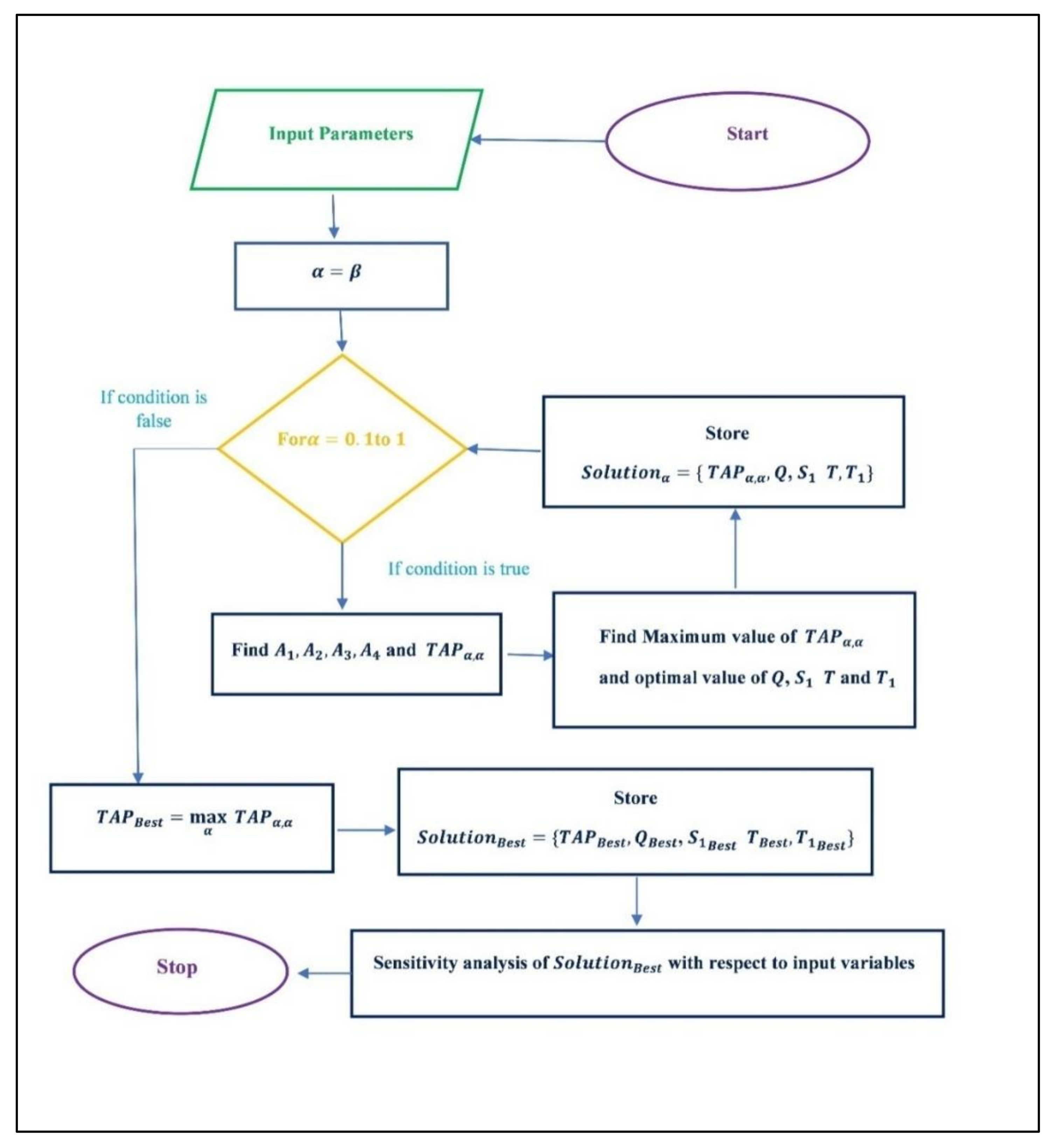
5.1. Solution Methodology

Here, the solution algorithm is first structured before going for the numerical simulation of the proposed model. The below is the algorithm in brief to solve the problem.

Algorithm 1

Step 1: Start

Step 2: Initialize input variable $a$, $b,c,h_c,s_c,S_{up}$ and $p$

Step 3: Set $\alpha =\beta$

Step 4: Check “for” condition

Step 5: If “for” condition is validated go to Step 5, otherwise go to Step 9

Step 6: Evaluate $A_1=E_{\alpha }\left(-c{T}_1{}^{\alpha }\right)$, $A_2=\mathsf{\Gamma }\left(\alpha +1\right)$, $A_3=\frac{\left(\frac{1}{A_1}-\frac{c{T}_1{}^{\alpha }}{A_2}-1\right)}{c}$, $A_4=\frac{s_c{\left(T-T_1\right)}^{2\alpha }}{\mathsf{\Gamma }\left(2\alpha +1\right)}$ and $TA{P}_{\alpha ,\alpha }=\frac{\left(a-bp\right)}{T}\left[\frac{p{T}_1{}^{\alpha }}{\mathsf{\Gamma }\left(\alpha +1\right)}+\left(p-\frac{h_c}{c}\right)A_3-A_4\right]-\frac{S_{up}}{T}$

Step 7: Find Maximum value of $TA{P}_{\alpha ,\alpha }$ and optimal value of $Q$, $S_1$, $T$ and $T_1$

Step 8: Store $Solutio{n}_{\alpha }=\{ TA{P}_{\alpha ,\alpha },Q$, $S_{1}T, T_1\}$

Step 9: Go to Step 3

Step 10: $TA{P}_{Best}=\underset{\alpha }{\max } TA{P}_{\alpha ,\alpha }$

Step 11: Store $Solutio{n}_{Best}=\left\{TA{P}_{Best},Q_{Best}, S_1{}_{Best}{T}_{Best}, T_1{}_{Best}\right\}$

Step 12: Sensitivity analysis of $Solutio{n}_{Best}$ with respect to input variables

Figure 2 depicts the solution methodology in a flow chart which would be used in next sub sections for the numerical optimization of the proposed economic order quantity model.

5.2. Numerical Simulation

The algorithm mentioned in the preceding subsection is coded in the Mathematica software. For numerical illustration, let us take the values of the parameters involved in defining the proposed inventory as follows:

$a=200$, $b=1.5$, $c=0.005$, $h_c=0.5$, $s_c=0.25$, $S_{up}=1000$ and $p=5$.

The solutions to the optimization problems are given in tabular forms. Here, the model’s two cases, namely, shortage and without shortage, are described.

Table 4. Impact memory on optimum values of the objective function total average profit ($TA{P}^{*}$), and decision variables, namely.initial inventory level ($S_1$), lot size ($Q$), active inventory run phase ($T_1$), total lot cycle ($T$) for the model with shortage.

Memory Index	${\mathit{T}}^{*}$	${\mathit{T}}_1{}^{*}$	${\mathit{Q}}^{*}$	${\mathit{S}}_1{}^{*}$	$\mathit{T}\mathit{A}{\mathit{P}}^{*}$
1	3.762	3.762	731.02	731.02	432.51
0.9	6.303	3.373	603.02	1128.65	187.98
0.8	6.303	3.373	549.73	1038.12	174.83
0.7	6.303	3.373	498.35	947.94	157.93
0.6	6.303	3.373	448.26	856.87	137.81
0.5	3.392	3.392	400.95	400.95	256.84
0.4	6.303	3.373	419.03	752.54	90.41
0.3	6.303	3.373	309.14	605.26	64.51
0.2	6.303	3.373	267.46	527.40	38.10
0.1	5.120	3.574	229.85	441.20	17.41

represents the optimal solution concerning different memory index values for the proposed model with the shortage.

Table 5. Impact memory on optimum values of the objective function total average profit ($TA{P}^{*}$), and decision variables, namely,lot size ($Q$), total lot cycle ($T$) for the model without shortage.

Memory Index	${\mathit{T}}^{*}$	${\mathit{Q}}^{*}$	$\mathit{T}\mathit{A}{\mathit{P}}^{*}$
1	3.762	731.02	432.51
0.9	3.971	698.10	415.29
0.8	4.085	641.35	387.56
0.7	4.016	563.39	350.12
0.6	3.755	478.17	305.56
0.5	3.392	400.95	256.84
0.4	3.024	338.24	205.86
0.3	2.710	289.47	153.29
0.2	2.498	251.86	98.91
0.1	2.607	222.71	42.50

depicts the same for the model without shortage.

Remark 4. The value of the memory index near 0 and 1 represent strong and weak memory senses, respectively. Therefore, the memory sense is becoming firmer from top to bottom in Table 4. The total average profit gradually decreases as memory strengthens. The optimal lot size is also following the same trend. However, the whole lot cycle, active lot cycle, and initial stock level have no uniform tendency from top to bottom in Table 4. The shortage phase is diminishing for the corresponding memory index values equal to 1 and 0.5.

Remark 5. From Table 5, it is perceived that the total average profit gradually decreases as memory strengthens. The optimal lot size is also following the same trend. However, the lot cycle has no uniform tendency from top to bottom in Table 5.

Remark 6.Using the tabular data from Table 4 and Table 5, the variation of total average profit, lot cycle, and lot size concerning the variation of the memory index is plotted in Figure 3, Figure 4 and Figure 5, respectively, for both the cases of shortage and without shortage. On the other hand, the relational dependences of the total average profit and lot cycle for the shortage and without shortage are depicted in Figure 6 and Figure 7, respectively. The three-dimensional dependencies among the memory index, lot size and total average profit for the cases of shortage and without shortage are shown in Figure 8 and Figure 9, respectively. Figure 10 and Figure 11 depict the relational dependence of lot cycle, lot size and total average profit for the cases of shortage and without shortage, respectively.

Note 1. The lower value of the memory index stands for the strong memory sense of the system. As the memory index approaches 1, the system becomes memory-free. If we focus on the profit maximization objective of the retailer, from the tabular and graphical representation in the present subsection, it has been established that the memory-free phenomenon is most desirable to attain the maximum gain. The system memory causes the retailing activities negatively. The most desirable phenomenon is obtained for $\alpha =\beta =1$ and then the optimal values of the objective function and decision parameters are $TA{P}^{*}=USD 432.51, Q^{*}=S_1{}^{*}=731.02$ unit and $T^{*}=T_1{}^{*}=3.762\mathrm{months}$. Additionally, it is seen that for $\alpha =\beta$, the optimal values of the objective function and decision parameters coincide.

5.3. Sensitivity Analysis

In this subsection, we make a sensitive analysis of the best-desired result according to the retailer’s perspective to the different input parameters. In

Table 6. Sensitivity analysis on optimum values of the objective function total average profit ($TA{P}^{*}$), and decision variables, namely.initial inventory level ($S_1$), lot size ($Q$), active inventory run phase ($T_1$), total lot cycle ($T$) for the model with shortage with respect to the input variables ($S_{up}$, $h_c$, $p$, $s_c$, $c$) varying them from −50% to +50% of their values.

Parameters	Percentage	${\mathit{T}}_1{}^{*}$	${\mathit{T}}^{*}$	${\mathit{Q}}^{*}$	${\mathit{S}}_1{}^{*}$	$\mathit{T}\mathit{A}{\mathit{P}}^{*}$
$S_{up}$	+50	4.601	4.601	895.34	895.34	312.94
	+30	4.285	4.285	833.85	833.85	357.96
	+10	3.994	3.994	766.81	766.81	406.56
	−10	3.570	3.570	693.39	693.39	459.79
	−30	3.151	3.151	611.30	611.30	515.31
	−50	2.665	2.665	516.43	516.43	588.09
$h_c$	+50	3.058	3.058	593.12	593.12	310.07
	+30	3.289	3.289	638.35	638.35	356.06
	+10	3.582	3.582	695.80	695.80	405.86
	−10	3.972	3.972	772.17	772.17	460.59
	−30	4.524	4.524	880.82	880.82	522.09
	−50	5.399	5.399	1053.56	1053.56	593.75
$p$	+50	3.832	3.832	730.23	730.23	895.34
	+30	3.804	3.804	730.55	730.55	712.46
	+10	3.776	3.776	730.86	730.86	512.58
	−10	3.748	3.748	731.17	731.17	337.70
	−30	3.721	3.721	731.48	731.48	145.82
	−50	4.550	3.658	724.58	899.60	−43.76
$s_c$	+50	3.762	3.762	731.02	731.02	432.51
	+30	3.762	3.762	731.02	731.02	432.51
	+10	3.762	3.762	731.02	731.02	432.51
	−10	3.762	3.762	731.02	731.02	432.51
	−30	3.762	3.762	731.02	731.02	432.51
	−50	3.762	3.762	731.02	731.02	432.51
$c$	+50	3.783	3.783	738.59	738.59	436.26
	+30	3.774	3.774	735.53	735.53	434.75
	+10	3.766	3.766	732.51	732.51	433.26
	−10	3.758	3.758	729.53	729.53	431.77
	−30	3.750	3.750	726.57	726.57	430.29
	−50	3.742	3.742	723.65	723.65	428.81

, the values of the onetime setup, unit holding cost, unit shortage cost, selling price and stock coefficient vary from −50% to +50% and the effect of the variations on the optimal solution is displayed. The total average profit is the most significant issue for the retailers.

Remark 7. In Figure 12 we see that the overall average profit steadily drops as the setup and holding expenses rise from −50% to 50% of their value. On the other hand, the total average profit rises as the selling price steadily climb from 50% to 50% of its worth, spanning a wide range of values. The influence of the stock coefficient in the demand function is also somewhat less critical on the sensitivity analysis of the profit function, in addition to the unit shortage cost’s negligible impact on the sensitivity of the best solution.

5.4. Major Observations

From the numerical simulation of the preceding two subsections, we observe the following significant points:

For both shortage and without shortage cases, as the value of the memory index increases, the value of the total average profit increases. Mathematically, the fractional value of the memory index near zero implies a strong memory sense. On the other hand, the memory index values near one stand for the weak memory sense. Thus, the numerical simulation of this section implies that poor memory sense is more desirable for boosting profitability in favor of the retailer’s goal.

(i)

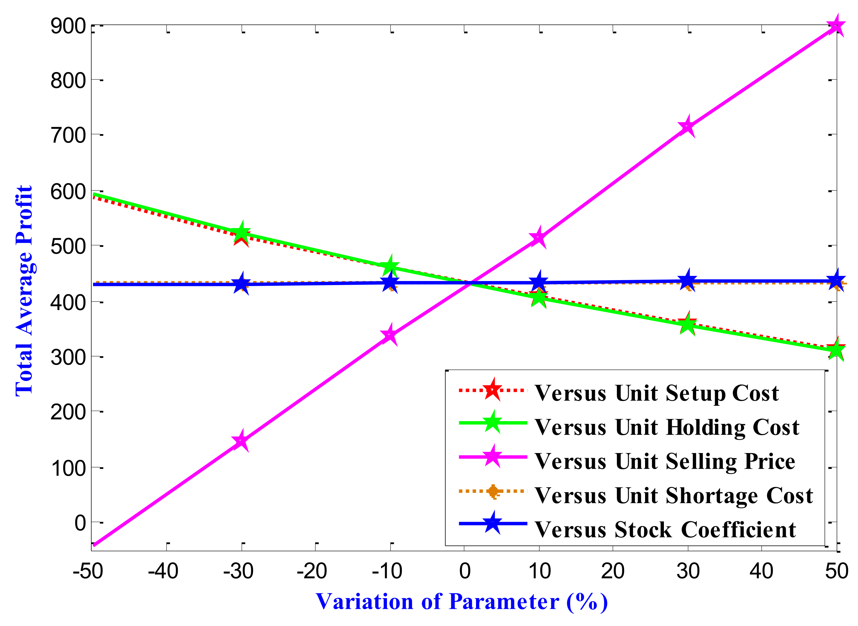
As the memory index approaches to value 1 (towards the memory less situation), the model with the shortage coincides with the model without shortage. Thus, there is no such effect of the unit shortage cost on the average profit function. Thus, the sensitivity curve of the average profit to the unit shortage cost is displayed as a straight line in Figure 12.

(ii)

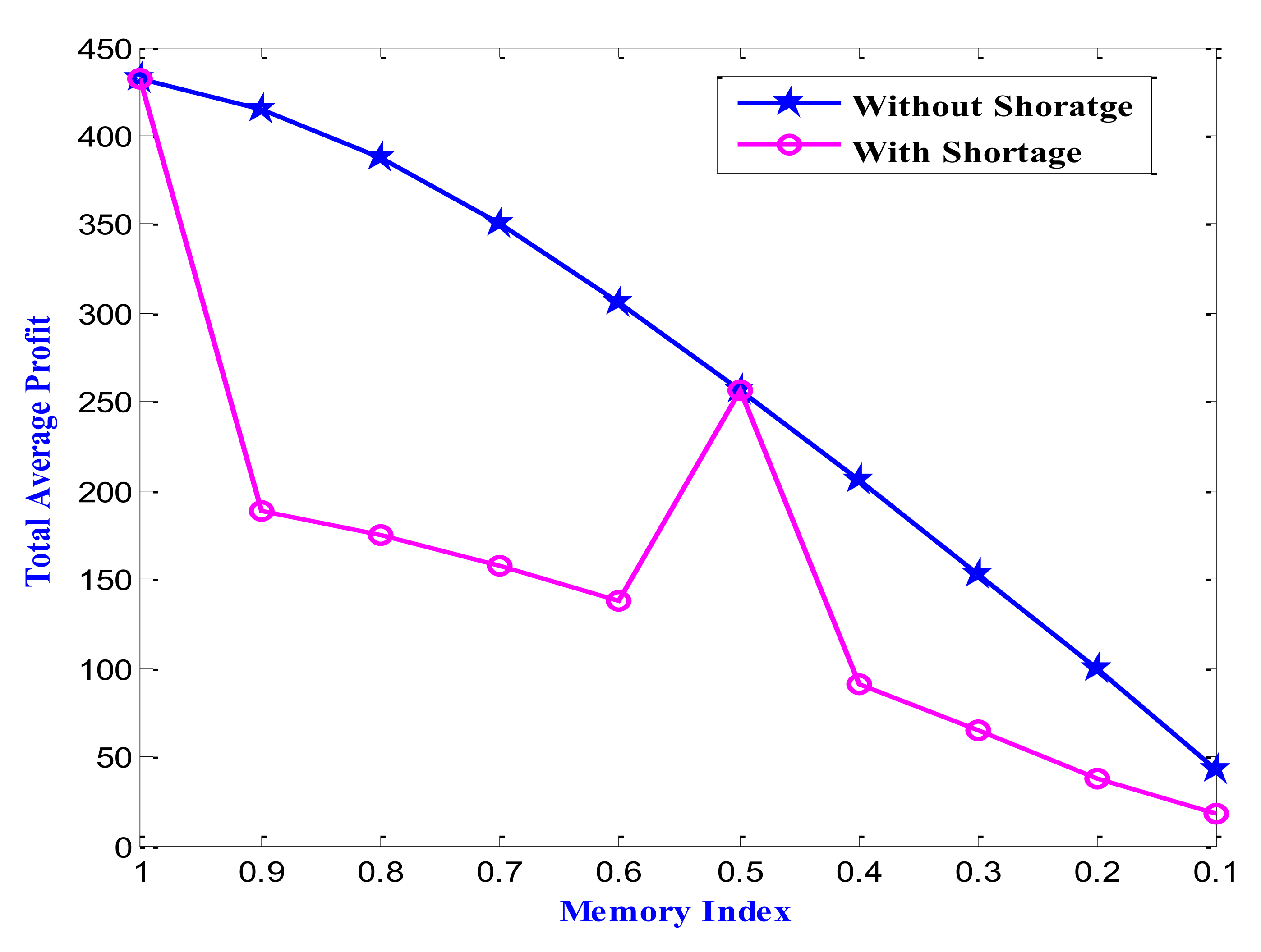
The medium memory sense is given by the value of the memory index near 0.5. For medium memory sense, the models with and without shortage again converge to one.

(iii)

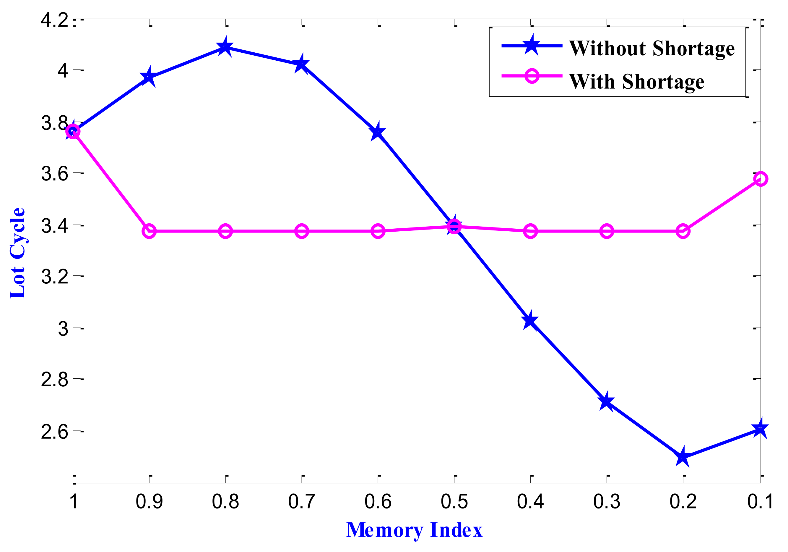
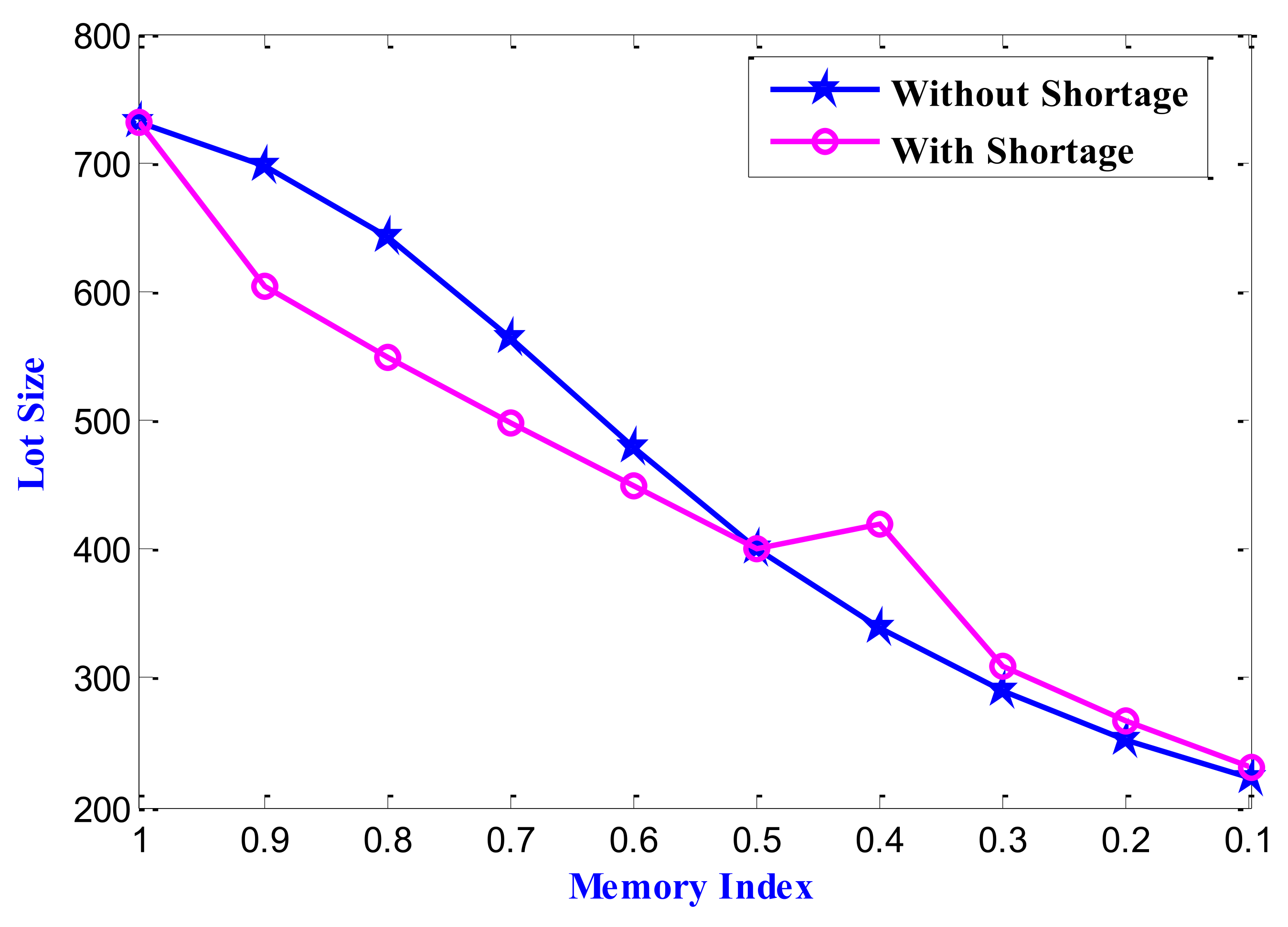
The span of the lot cycle decreases uniformly with an exception at the value of the memory index near zero as the memory sense is more vital for the case of a model without shortage. For the case of shortage, the span of the lot cycle is a little bit high for the memory index nearer to both the extreme ends that is 0 and 1. The graph is almost a straight line in the memory index’s other intermediate values.

(iv)

The lot sizes for both models face gradual uniform decay as the memory becomes more robust. The curves representing the two models coincide for the memory index values equal to 0.5 and 1.

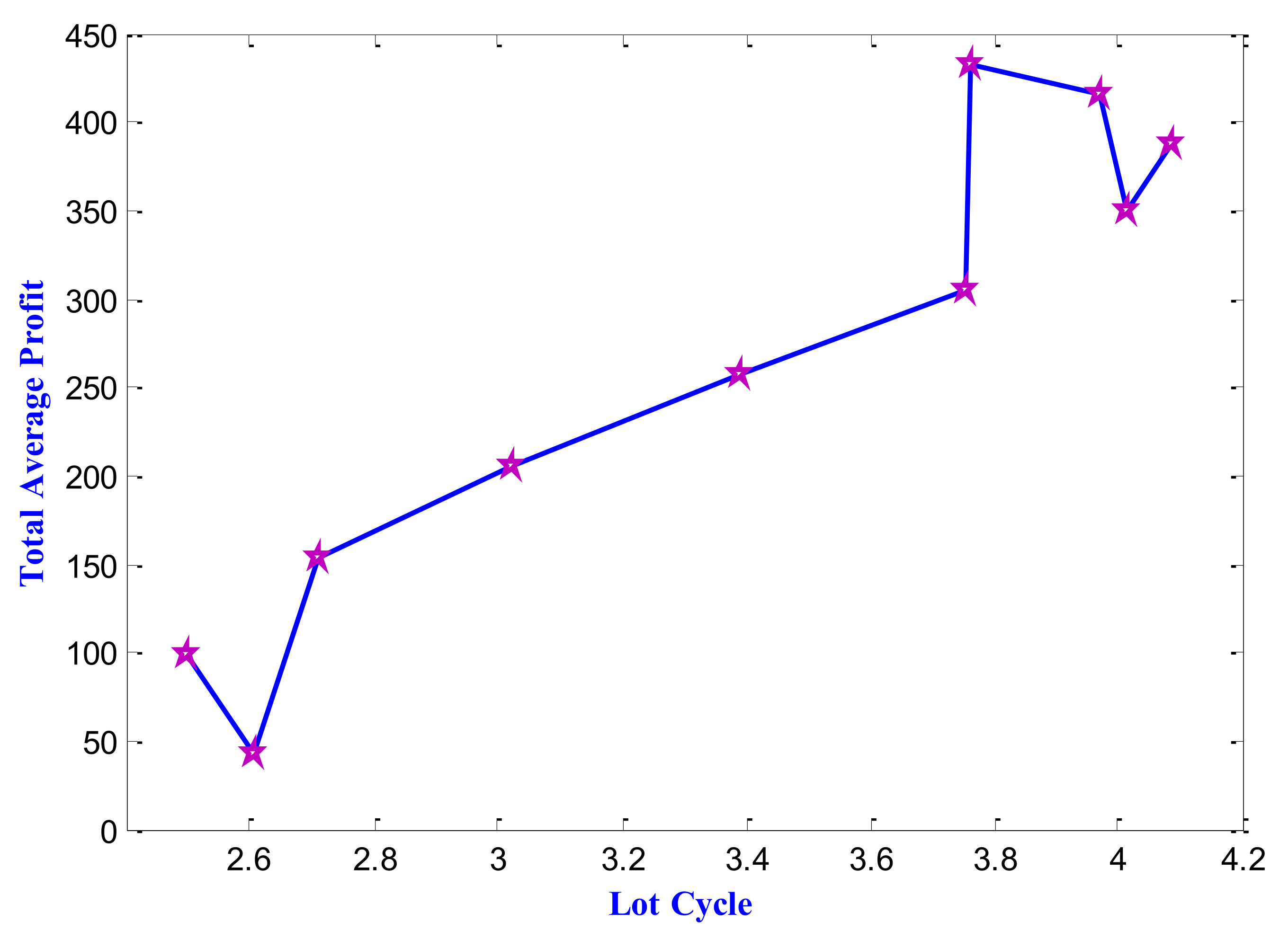
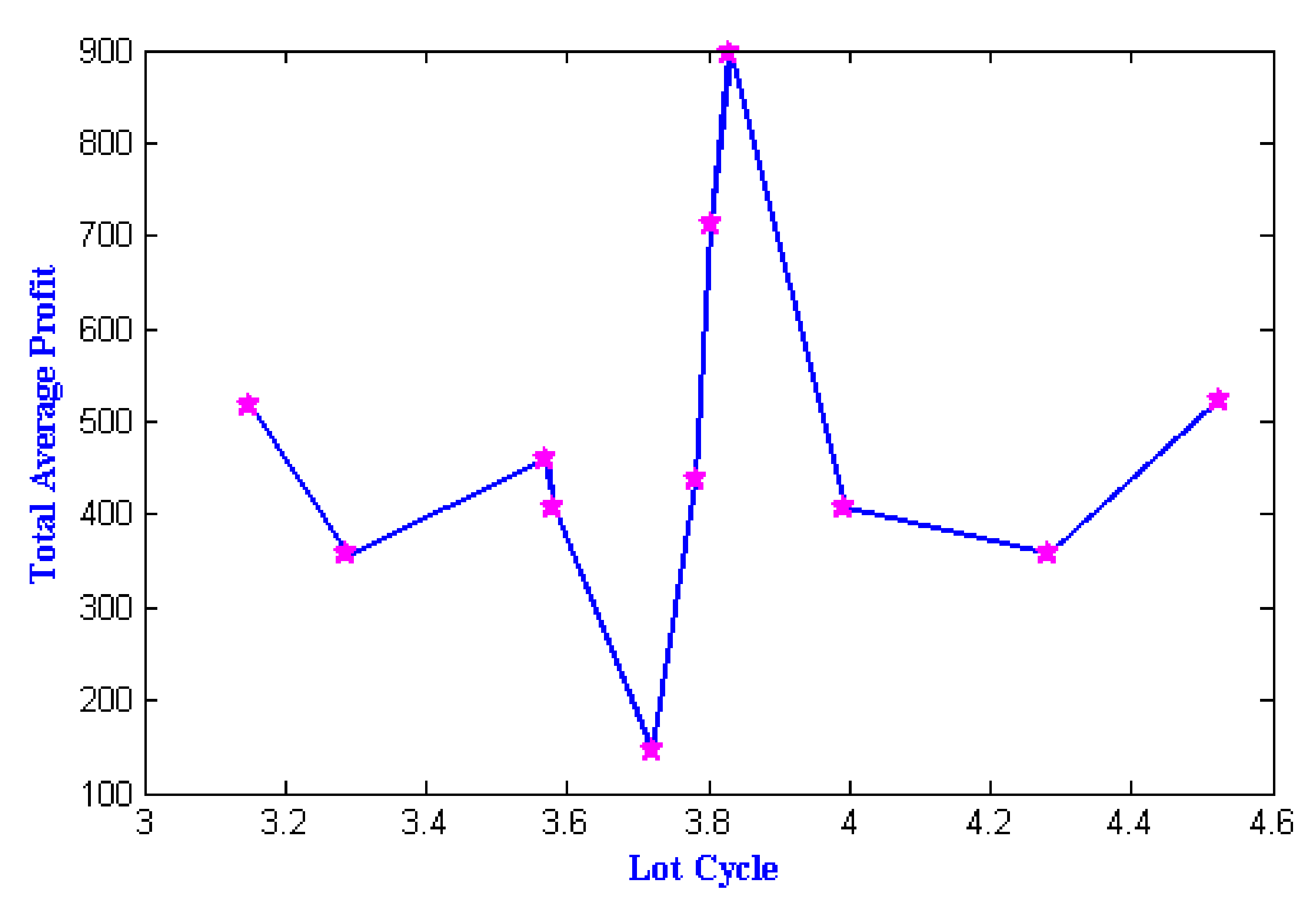
(v)

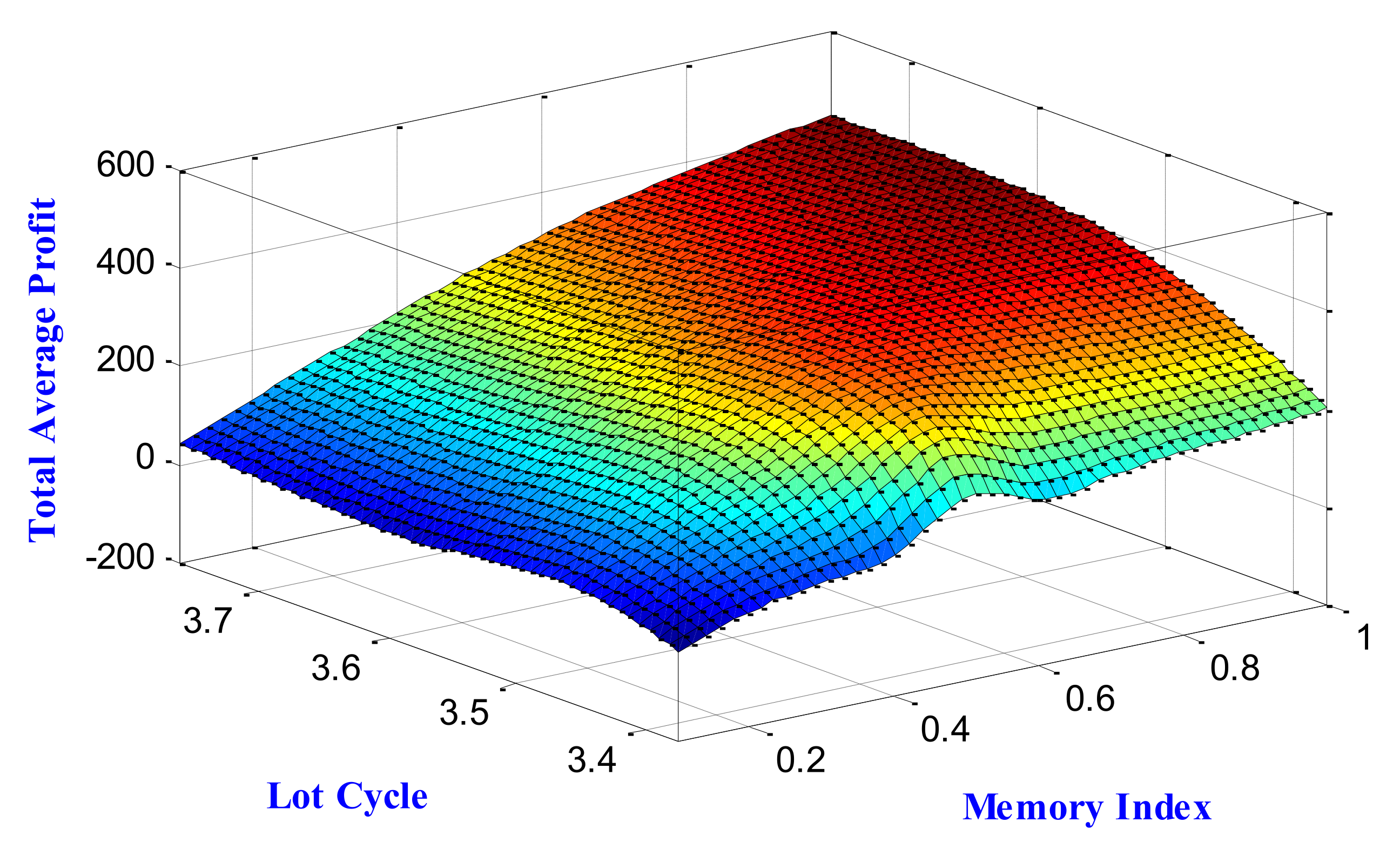
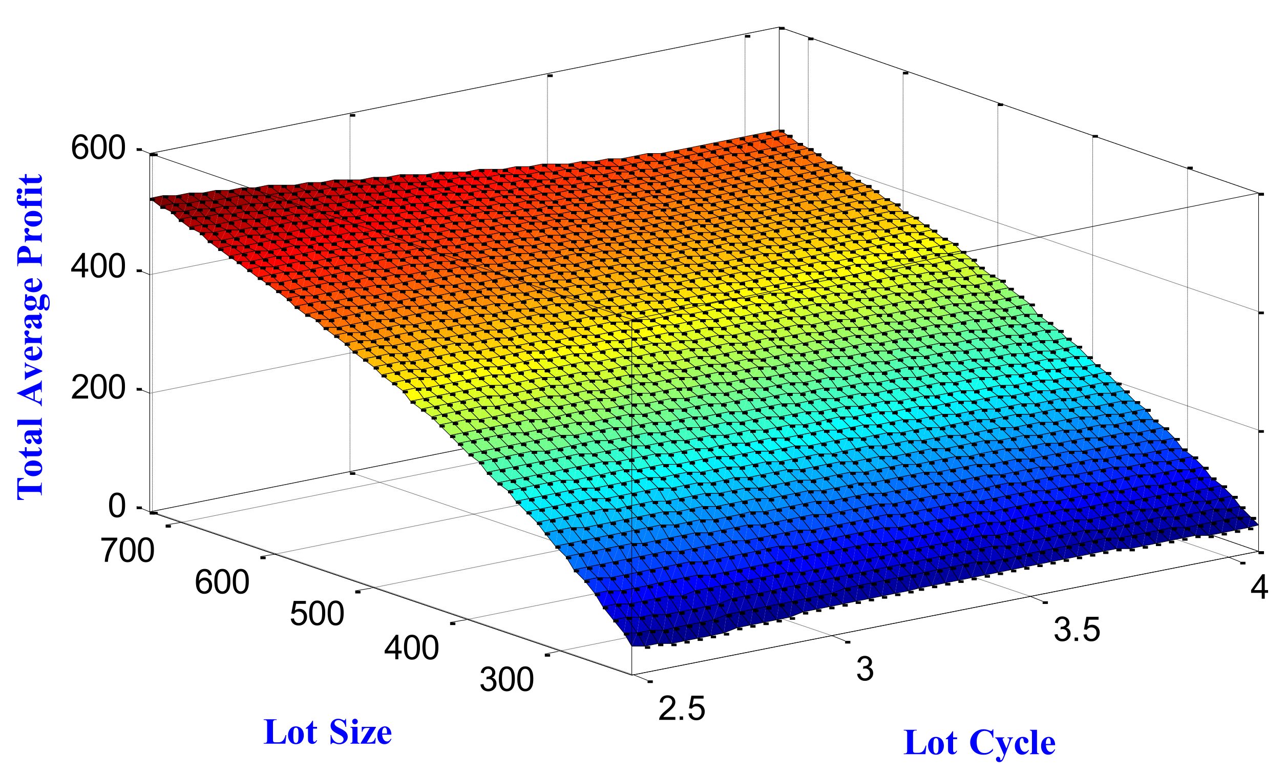
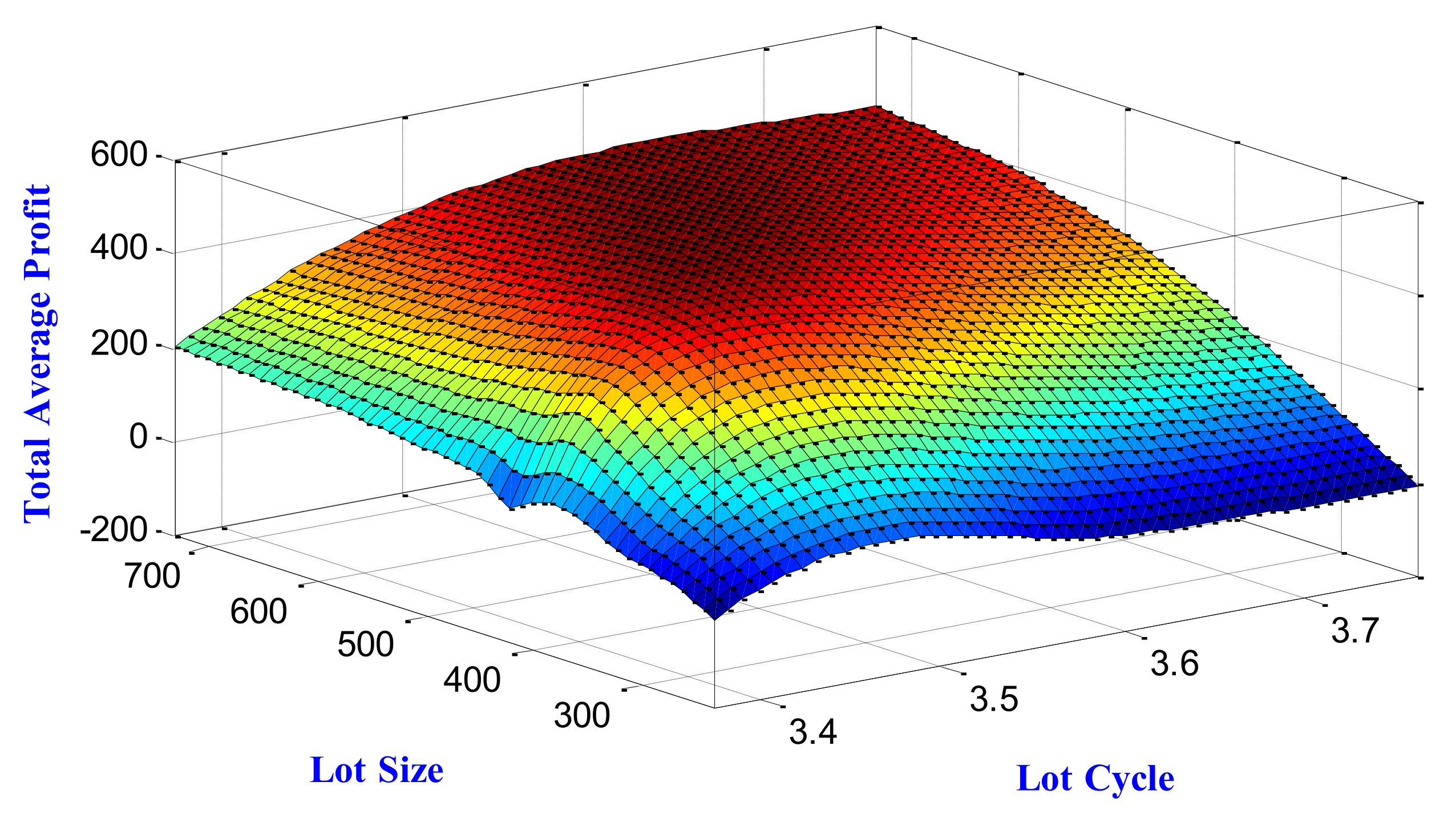
The variation of the total average profit against the lot cycle is not uniform. For both the cases of shortage and without shortage, it faces several up and down in the curve plotting. Because of the effect of memory, there is no such straightforward relation between the average profit and lot cycle.

(vi)

As the setup and holding costs gradually increase from −50% to 50% of its value, the total average profit decreases moderately. The outcome is quite evident.

(vii)

The unit selling price has seemed the most crucial input parameter, which significantly impacts the sensitivity of the optimal solution. As the selling price gradually increases from −50% to 50%of its value, the total average profit increases, covering a vast range of values.

(viii)

Apart from the insignificant role of the unit shortage cost on the sensitivity of the optimal solution (reasons are discussed earlier), the impact of the stock coefficient in the demand function is also slightly inferior on the sensitivity analysis of the profit function. This is because we restrict our model to be developed under the assumption that the demand is dependent on the displayed stock, but not so much.

6. Managerial Insights and Real-Life Applications

The following two subsections highlight the suggested model’s managerial insights and application domains in this section’s actual scenarios.

6.1. Managerial Insights

We consider the demand of the suggested EOQ model to be a function of selling price and displayed stock while formulating the model. The memory-sensitive environment is assured by using fractional calculus as a mathematical tool. The numerical results have shown the following managerial lessons:

• A person involved in the situation cannot be memory-free. Because of the interactions between retailers and customers during earlier transactions, there must be some system memory that might play a part in the current scenario. It has been determined through the models’ numerical simulation that the memory negatively impacts the retailer’s objective of maximum gain. The retailer’s objective may be accomplished in a nearly memory-free setting. The absence of memory is the ideal circumstance for increased profitability, but this is not always feasible in practice.
• The selling price and demand are inversely correlated. On the other hand, the numerical results show that raising the selling price will maximize the profit. The selling price’s influence on the profit function outweighs its influence on the demand function.
• The showroom’s merchandise display may help favorably draw customers’ attention. However, in practice, this effect is not comparable to the mania surrounding the instance of decreasing the selling price. Numerical optimization assumes that the stock component of the demand function has low values. The result is a favorable but marginally less significant influence of the presented stock on the profit target.
• Another intriguing finding from the numerical results is that the retailer’s purpose in a memory-free environment is best served by the convergence of the models with and without shortage. The highest average profit may be achieved when there is no shortage and no memory constraints.

6.2. Possible Domains of Application

6.2.1. Retail Bakery Inventory

Baking is the process in which foods are cooked by dry heat. Bread, cookies, biscuits, rolls, cakes, cupcakes, pies, tarts, and sweet rolls are bakery products. Bakery goods such as bread and biscuits supply essential nutrients for maintaining health through a balanced diet. Thus, stock, retail and its coordination management are matters of significant concern. The demand for the baked product must be price sensitive. The low-priced product must have high demand. The impact of displayed stocks in the store on the market and thus on the profit is slightly inferior. Therefore, the assumptions of the proposed model are highly relatable to the scenario of the retail bakery inventory. In the proposed model, it is observed that large memory negatively impacts the EOQ model’s profitability. Furthermore, the model advocates for the scenario of no shortage. So, one can apply the proposed decision-making problem to the retail bakery inventory in which the better retailing goal can be achieved with a fresh start (low memory) and tight supply flow (no shortage).

6.2.2. Chicken Retail Store

Chicken production and its consumption rate appear to be rapid day by day. Opening a chicken retail store is a straightforward and profitable job. The low price of the slaughtered chicken can attract the consumer’s attention and may increase the profitability in favor of the retailer’s side. However, the mass or the number of poultry impacts neither the demand rate nor the average profit. So, the proposed retail design fits the chicken retail scenario well. The managerial insights given by the present paper to the actual chicken retail store is that the retail body can achieve its goal of better gain with a fresh start (low memory) and tight supply flow (no shortage).

7. Conclusions and Future Research Scope

This paper presents a mathematical approach for designing a memory-sensitive decision-making environment for an EOQ model. We assume that demand is a linear function of selling price and displayed. The lot-sizing model is considered for both cases of shortage and without shortage. The fractional calculus theory is used to demonstrate the memory-inspired EOQ model. Initially, the traditional EOQ model was developed in a memory-free environment. Then, the memory in terms of iterative impact has been supplied to the model to design its fractional counterpart. Intuitively, the association of fractional calculus with this present study is not only for representing a memory-based decision scenario; it also includes the memory-free traditional approach of lot size modeling as a particular case.

Based on the theoretical advancement, a solution algorithm of the optimization model equivalent to the proposed EOQ is designed and solved in Mathematica software for numerical analysis. The results suggest that the system memory negatively impacts the profit maximization objective. The memory-free situation is the most desired phenomenon from the retailer’s side. Additionally, the numerical results show that maintaining a continuous supply free of any shortfall will yield the most profit.

The proposed mathematical model is suitable for a business phenomenon where the retailing organization is newly introduced and the showroom is not well built yet. The small-scale retailing store of bakery and chicken slaughtering may be viewed as domains of application for the prescribed mathematical model in this paper.

The present study has some limitations. We consider an EOQ model with minimal decision variables in a memory-motivated situation because of the complexity of dealing with the fractional-order system. The supply chain channels have more decision variables to control the objectivity of the models. One of the possible future extensions of this study is to incorporate the sense of memory in different junctions of supply chain models so that an accurate picture of memory impact on the supply chain will reveal. We can construct the model by considering the non-linear dependency, for example, the application of logistic differential equation, between some factors and proceed further in the future. The theory of fractional calculus may need to be improved to do this, emphasizing its applications in operation research. Additionally, the analytical approach may be replaced by fruitful soft computing techniques for numerical optimization of fractional lot-sizing problems.

References

1. Taleizadeh, A.A.; Nematollahi, M. An inventory control problem for deteriorating items with back ordering and financial considerations. Appl. Math. Model. 2014, 38, 93–109. [Google Scholar] [CrossRef]
2. Taleizadeh, A.A.; Stojkovska, I.; Pentico, D.W. An economic order quantity model with partial back ordering and increment discount. Comput. Ind. Eng. 2015, 82, 21–32. [Google Scholar] [CrossRef]
3. Taleizadeh, A.A. Lot sizing Model with advance payment pricing and disruption in supply under planned partial back ordering. Int. Trans. Oper. Res. 2017, 24, 783–800. [Google Scholar] [CrossRef]
4. Salehi, H.; Taleizadeh, A.A.; Tavakkoli-Moghaddam, R. An EOQ model with random disruption and partial backordering. Int. J. Prod. Res. 2016, 54, 2600–2609. [Google Scholar] [CrossRef]
5. Lashgari, M.; Taleizadeh, A.A.; Sana, S.S. An inventory control problem for deteriorating items with back ordering and financial considerations under two level of trade credit linked to order quantity. J. Ind. Manag. Optim. 2016, 12, 1091–1119. [Google Scholar] [CrossRef]
6. Das, S. Functional Fractional Calculus for System Identification and Controls; Springer: Berlin/Heidelberg, Germany; New York, NY, USA, 2008. [Google Scholar]
7. Jumarie, G. Modified Riemann–Liouville derivative and fractional Taylor series non differentiable functions further results. Comput. Math. Appl. 2006, 51, 1367–1376. [Google Scholar] [CrossRef]
8. Saeedian, M.; Khalighi, M.; Azimi-Tafreshi, N.; Jafari, G.R.; Ausloos, M. Memory effects on epidemic evolution: The susceptible-infected-recovered epidemic model. Phys. Rev. 2017, 95, 022409. [Google Scholar] [CrossRef]
9. Tarasov, V.E.; Tarasova, V.V. Phillips model with exponentially distributed lag and power-law memory. Comput. Appl. Math. 2019, 38, 13. [Google Scholar] [CrossRef]
10. Tarasova, V.V.; Tarasov, V.E. Memory effects in hereditary Keynesian model. Prob. Mod. Sci. Edu. 2016, 38, 38–44. [Google Scholar] [CrossRef]
11. Tarasov, V.E.; Tarasova, V.V. Long and short memory in economics: Fractional-order difference and differentiation. IRA Int. J. Manag. Soc. Sci. 2016, 5, 327–334. [Google Scholar] [CrossRef] [Green Version]
12. Debnath, L. Recent applications of fractional calculus to science and engineering. Int. J. Math. Math. Sci. 2003, 2003, 3413–3442. [Google Scholar] [CrossRef]
13. Odzijewicz, T.; Malinowska, A.B.; Toores, D.F.M. Fractional calculus of variation in terms of a generalized fractional integral with Applications to physics. In Abstract and Applied Analysis; Hindawi: London, UK, 2012; pp. 1–24. [Google Scholar]
14. Chen, W.C. Nonlinear dynamics and chaos in a fractional-order financial system. Chaos Solitons Fractals 2008, 36, 1305–1314. [Google Scholar] [CrossRef]
15. Abdeljawad, T.; Baleanu, D. Caputo q-fractional initial value problems and a q-analogue Mittag–Leffler function. Commun. Nonlinear Sci. Numer. Simul. 2011, 16, 4682–4688. [Google Scholar] [CrossRef]
16. Ahmad, B.; Nieto, J.J. Boundary value problems for a class of sequential integrodifferential equations of fractional order. J. Funct. Spaces 2013, 2013, 149659. [Google Scholar] [CrossRef]
17. Agarwal, R.P.; Lakshmikantham, V.; Nieto, J.J. On the concept of solution for fractional differential equations with uncertainty. Nonlinear Anal. Theory Methods Appl. 2010, 72, 2859–2862. [Google Scholar] [CrossRef]
18. Salahshour, S.; Allahviranloo, T.; Abbasbandy, S. Solving fuzzy fractional differential equations by fuzzy Laplace transforms. Commun. Nonlinear Sci. Numer. Simul. 2012, 17, 1372–1381. [Google Scholar] [CrossRef]
19. Du, M.; Wang, Z.; Hu, H. Measuring memory with the order of fractional derivative. Sci. Rep. 2013, 3, 3431. [Google Scholar] [CrossRef]
20. Transchel, S.; Mirner, S. Coordinated lot-sizing and dynamic pricing under a supplier all-units quantity discount. Bus. Res. 2008, 1, 125–141. [Google Scholar] [CrossRef]
21. Sana, S.S. Price sensitive demand and random sales price- a news boy problem. Int. J. Sys. Sci. 2012, 43, 491–498. [Google Scholar] [CrossRef]
22. Pal, B.; Sana, S.S.; Chaudhuri, K. Two echelon manufactures retailer supply chain strategies with price, quality and promotional effort sensitive demand. Int. Trans. Oper. Res. 2015, 22, 1071–1095. [Google Scholar] [CrossRef]
23. Alfares, H.K.; Ghaithan, A.M. Inventory and pricing model with price-dependent demand, time varying holding cost and quantity discounts. Comput. Ind. Eng. 2016, 94, 170–177. [Google Scholar] [CrossRef]
24. Das, S.C.; Zidan, A.M.; Manna, A.K.; Shaikh, A.A.; Bhunia, A.K. An application of preservation technology in inventory control system with price dependent demand and partial backlogging. Alex. Eng. J. 2020, 59, 1359–1369. [Google Scholar]
25. Rahman, M.S.; Duary, A.; Shaikh, A.A.; Bhunia, A.K. An application of parametric approach for interval differential equation in inventory model for deteriorating items with selling-price-dependent demand. Neural. Comput. Appl. 2020, 32, 14069–14085. [Google Scholar] [CrossRef]
26. Min, J.; Zhou, Y.W. A perishable inventory model under stock-dependent selling rate and shortage-dependent partial backlogging with capacity constraint. Int. J. Sys Sci. 2009, 40, 33–44. [Google Scholar] [CrossRef]
27. Yang, H.L.; Teng, J.T.; Chern, M.S. An inventory model under inflation for deteriorating items with stock-dependent consumption rate and partial backlogging shortages. Int. J. Prod. Econ. 2010, 123, 8–19. [Google Scholar] [CrossRef]
28. Singh, S.R.; Kumar, N.; Kumari, R. An inventory model for deteriorating items with shortage and stock-dependent demand under inflation for two shops under one management. Opsearch 2010, 47, 311–329. [Google Scholar] [CrossRef]
29. Bhunia, A.; Shaikh, A.A. A deterministic model for deteriorating items with displayed inventory level dependent demand rate incorporating marketing decisions with transportation cost. Int. J. Ind. Eng. Comput. 2011, 2, 547–562. [Google Scholar] [CrossRef]
30. Lee, Y.P.; Dye, C.Y. An inventory model for deteriorating items under stock-dependent demand and controllable deterioration rate. Comput. Ind. Eng. 2012, 63, 474–482. [Google Scholar] [CrossRef]
31. Bhunia, A.K.; Mahato, S.K.; Shaikh, A.A.; Jaggi, C.K. A deteriorating inventory model with displayed stock-level-dependent demand and partially backlogged shortages with all unit discount facilities via particle swarm optimisation. Int. J. Sys. Sci. Oper. Logis. 2014, 1, 164–180. [Google Scholar] [CrossRef]
32. Shaikh, A.A.; Cárdenas-Barrón, L.E.; Tiwari, S. A two-warehouse inventory model for non-instantaneous deteriorating items with interval-valued inventory costs and stock-dependent demand under inflationary conditions. Neural. Comput. Appl. 2019, 31, 1931–1948. [Google Scholar] [CrossRef]
33. Panda, D.; Maiti, M.K.; Maiti, M. Two warehouse inventory model for single vendor multiple retailers with price and stock dependent demand. Appl. Math. Model. 2010, 34, 3571–3585. [Google Scholar] [CrossRef]
34. Dye, C.Y.; Hsieh, T.P. Deterministic ordering policy with price and stock dependent demand under fluctuating cost and limited capacity. Expert Syst. Appl. 2011, 38, 14976–14983. [Google Scholar] [CrossRef]
35. Sana, S.S. An EOQ model for salesman initiatives, stock and price dependent demand of similar products –a dynamical system. Appl. Math. Comput. 2011, 218, 3277–3288. [Google Scholar]
36. Giri, B.C.; Bardhan, S. Supply chain coordination for a deteriorating item with stock and price-dependent demand under revenue sharing contract. Int. Trans. Oper. Res. 2012, 19, 753–768. [Google Scholar] [CrossRef]
37. Sarkar, B.; Sarkar, S. An improved inventory model with partial backlogging, time varying deterioration and stock-dependent demand. Econ. Model. 2013, 30, 924–932. [Google Scholar] [CrossRef]
38. Pal, S.; Mohapatra, G.S.; Samanta, G.P. An inventory model of price and stock dependent demand rate with deterioration under inflation and delay in payments. Int. J. Sys. Assur. Eng. Manag. 2014, 5, 591–601. [Google Scholar] [CrossRef]
39. Mishra, U.; Barron, L.E.-C.; Tiwari, S.; Shaikh, A.A.; Graza, G.T. An inventory model under price and stock dependent demand for controllable deterioration rate with shortage and preservation technology investment. Ann. Oper. Res. 2017, 254, 165–190. [Google Scholar] [CrossRef]
40. Shaikh, A.A.; Mashud, A.H.M.; Uddin, M.S.; Khan, M.A.A. Non instantaneous deterioration inventory model with price and stock dependent demand for fully backlogged storage under inflation. Int. J. Bus. Forecast. Market. Intell. 2017, 3, 152–164. [Google Scholar]
41. Mashud, A.; Khan, M.; Uddin, M.; Islam, M. A non-instantaneous inventory model having different deterioration rates with stock and price dependent demand under partial backlogged shortage. Uncertain Supply Chain. Manag. 2018, 6, 49–64. [Google Scholar] [CrossRef]
42. Shaikh, A.A.; Khan, M.A.; Panda, G.; Konstanteras, I. Price discount facility in an EOQ model for deteriorating items with stock dependent demand and partial backlogging. Int. J. Trans. Oper. Res. 2019, 26, 1365–1395. [Google Scholar] [CrossRef]
43. Khan, M.A.A.; Shaikh, A.A.; Panda, G.C.; Konstantaras, I.; Cárdenas-Barrón, L.E. The effect of advance payment with discount facility on supply decisions of deteriorating products whose demand is both price and stock dependent. Int. L Trans. Oper. Res. 2020, 27, 1343–1367. [Google Scholar] [CrossRef]
44. Rahaman, M.; Maity, S.; De, S.K.; Mondal, S.P.; Alam, S. Solution of an Economic Production Quantity model using the generalized Hukuhara derivative approach. Sci. Iran. 2021. [Google Scholar] [CrossRef]
45. Rahaman, M.; Mondal, S.P.; Alam, S.; De, S.K. A study of a lock fuzzy EPQ model with deterioration and stock and unit selling price-dependent demand using preservation technology. Soft Comput. 2022, 26, 2721–2740. [Google Scholar] [CrossRef]
46. Das, A.K.; Roy, T.K. Role of fractional calculus to the generalized inventory model. J. Glob. Res. Comput. Sci. 2014, 5, 11–23. [Google Scholar]
47. Das, A.K.; Roy, T.K. Fractional Order EOQ Model with Linear Trend of Time-Dependent Demand. Int. J. Intell. Sys. Appl. 2015, 3, 44–53. [Google Scholar] [CrossRef]
48. Pakhira, R.; Ghosh, U.; Sarkar, S. Study of memory effect in an inventory model with linear demand and salvage value. Int. J. Appl. Eng. Res. 2018, 13, 14741–14751. [Google Scholar]
49. Pakhira, R.; Ghosh, U.; Sarkar, S. Application of Memory effects In an Inventory Model with Linear Demand and No shortage. Int. J. Res. Advent Technol. 2018, 6, 1853–1871. [Google Scholar]
50. Pakhira, R.; Ghosh, U.; Sarkar, S. Study of Memory Effects in an Inventory Model with quadratic type demand rate and salvage value. Appl. Math. Sci. 2019, 13, 209–223. [Google Scholar] [CrossRef]
51. Pakhira, R.; Ghosh, U.; Sarkar, S. Study of Memory Effects in a fuzzy EOQ Model with no shortage. Int. J. Intell. Sys. Appl. 2019, 11, 58–68. [Google Scholar] [CrossRef]
52. Pakhira, R.; Ghosh, U.; Sarkar, S. Study of memory effect between two memory dependent inventory models. J. Fract. Calc. Appl. 2020, 11, 203–218. [Google Scholar]
53. Pakhira, R.; Sarkar, S.; Ghosh, U. Study of memory effect in an inventory model for deteriorating items with partial backlogging. Comput. Ind. Eng. 2020, 148, 106705. [Google Scholar] [CrossRef]
54. Rahaman, M.; Mondal, S.P.; Alam, S.; Goswami, A. Synergetic study of inventory management problem in uncertain environment based on memory and learning effects. Sādhanā 2021, 46, 39. [Google Scholar] [CrossRef]
55. Rahaman, M.; Mondal, S.P.; Alam, S. An estimation of effects of memory and learning experience on the EOQ model with price dependent demand. RAIRO Oper. Res. 2021, 55, 2991–3020. [Google Scholar] [CrossRef]
56. Rahaman, M.; Mondal, S.P.; Chatterjee, B.; Alam, S.; Shaikh, A.A. Generalization of Classical Fuzzy Economic Order Quantity Model Based on Memory Dependency via Fuzzy Fractional Differential Equation Approach. J. Uncertain Sys. 2022, 15, 2250003. [Google Scholar] [CrossRef]
57. Tsoularis, A. Deterministic and stochastic optimal inventory control with logistic stock-dependent demand rate. Int. J. Math. Oper. Res. 2014, 6, 41–69. [Google Scholar] [CrossRef]
58. Area, I.; Nieto, J.J. Fractional-Order Logistic Differential Equation with Mittag–Leffler-Type Kernel. Fractal Fract. 2021, 5, 273. [Google Scholar] [CrossRef]
Figure 1. Visual representation of the construction of the present paper with different sections and subsections.
Fractalfract 06 00531 g001
Figure 2. Flow chart of the solution algorithm for numerical simulation of the proposed model.
Fractalfract 06 00531 g002
Figure 3. Impact memory on optimum values of the objective function total average profit ( T A P * ) for the model with and without shortage (from left to right in the horizontal axis memory sense increases).
Fractalfract 06 00531 g003
Figure 4. Impact memory on optimum values of the decision variable lot cycle ( Q * ) for the model with and without shortage (from left to right in the horizontal axis memory sense increases).
Fractalfract 06 00531 g004
Figure 5. Impact memory on optimum values of the decision variable lot size ( T * ) for the model with and without shortage (from left to right in the horizontal axis memory sense increases).
Fractalfract 06 00531 g005
Figure 6. Variation of optimum values of the objective function total average profit ( T A P * ) with respect to the decision variable lot cycle ( Q * ) for the model without shortage.
Fractalfract 06 00531 g006
Figure 7. Variation of optimum values of the objective function total average profit ( T A P * ) with respect to the decision variable lot cycle ( Q * ) for the model with shortage.
Fractalfract 06 00531 g007
Figure 8. Three-dimensional dependency among total average profit, lot cycle and memory index for the case of no shortage.
Fractalfract 06 00531 g008
Figure 9. Three-dimensional dependency among total average profit, lot cycle and memory index for the case of shortage.
Fractalfract 06 00531 g009
Figure 10. Three-dimensional dependency among total average profit, lot cycle and lot size for the case of no shortage.
Fractalfract 06 00531 g010
Figure 11. Three-dimensional dependency among total average profit, lot cycle and lot size for the case of shortage.
Fractalfract 06 00531 g011
Figure 12. Graphs of the sensitivity analysis on optimum values of the objective function total average profit ( T A P * ) for the model with shortage with respect to the input variables ( S u p , h c , p , s c , c ) varying them from −50% to +50% of their values.
Fractalfract 06 00531 g012