Discriminant and Root Trajectories of Characteristic Equation of Fractional Vibration Equation and Their Effects on Solution Components

Abstract

The impulsive response of the fractional vibration equation $z^{\prime \prime }\left(t\right)+b{D}_t^{\alpha }z\left(t\right)+cz\left(t\right)=F\left(t\right)$, $b>0,c>0,0\le \alpha \le 2$, is investigated by using the complex path-integral formula of the inverse Laplace transform. Similar to the integer-order case, the roots of the characteristic equation $s^2+b{s}^{\alpha }+c=0$ must be considered. It is proved that for any $b>0$, $c>0$ and $\alpha \in (0,1)\cup (1,2)$, the characteristic equation always has a pair of conjugated simple complex roots with a negative real part on the principal Riemann surface. Particular attention is paid to the problem as to how the couple conjugated complex roots approach the two roots of the integer case $\alpha =1$, especially to the two different real roots in the case of $b^2-4c>0$. On the upper-half complex plane, the root $s\left(\alpha \right)$ is investigated as a function of order $\alpha$ and with parameters b and c, and so are the argument $\theta \left(\alpha \right)$, modulus $r\left(\alpha \right)$, real part $\lambda \left(\alpha \right)$ and imaginary part $\omega \left(\alpha \right)$ of the root $s\left(\alpha \right)$. For the three cases of the discriminant $b^2-4c$: $>0$, $=0$ and $<0$, variations of the argument and modulus of the roots according to $\alpha$ are clarified, and the trajectories of the roots are simulated. For the case of $b^2-4c<0$, the trajectories of the roots are further clarified according to the change rates of the argument, real part and imaginary part of root $s\left(\alpha \right)$ at $\alpha =1$. The solution components, i.e., the residue contribution and the Hankel integral contribution to the impulsive response, are distinguished for the three cases of the discriminant.

1. Introduction

In recent decades, fractional calculus has been followed with a lot of interest due to its ability as a mathematical tool to describe the memory and hereditary properties of various materials and processes [1,2,3,4,5,6,7,8]. The application areas relevant to fractional calculus are very extensive, including the viscoelastic constitutive relationship [4,7,9,10], anomalous diffusion [2,4], vibration and relaxation [2,4,7,8,11], control theory [2,5], stochastic process [12], etc. Let us recall the definitions in fractional calculus related to this paper.

Let $f\left(t\right)$ be piecewise continuous on $(0,+\infty )$ and integrable on any finite subinterval of $(0,+\infty )$. Then, the Riemann–Liouville fractional integral of $f\left(t\right)$ of order $\beta$ is defined as

$$\begin{array}{c}\hfill I_t^{\beta }f\left(t\right)={\int }_0^t\frac{{(t-\tau )}^{\beta -1}}{\mathsf{\Gamma }\left(\beta \right)}f\left(\tau \right)d\tau ,t>0,\end{array}$$

for $\beta >0$, and $I_t^{0}f\left(t\right)=f\left(t\right)$ for $\beta =0$, where $\mathsf{\Gamma }(·)$ is the gamma function. Let $\alpha$ be a positive real number, $m-1<\alpha <m$, $m\in {\mathbb{N}}^{+}$. Then, the Riemann–Liouville and Caputo fractional derivatives of $f\left(t\right)$ of order $\alpha$ are defined as

$$\begin{array}{c}\hfill {}^R{D}_t^{\alpha }f\left(t\right)=\frac{d^m}{d{t}^m}\left(I_t^{m-\alpha }f\left(t\right)\right),t>0,\mathrm{and}{}^C{D}_t^{\alpha }f\left(t\right)=I_t^{m-\alpha }\left(f^{\left(m\right)}\left(t\right)\right),t>0,\end{array}$$

respectively.

Theoretical analyses and experimental simulations indicated that the stress–strain relationship of a viscoelastic body can be better characterized by using fractional constitutive equations, such as the Scott–Blair model [4,9], the Kelvin–Voigt, Maxwell and Zener models [10,13,14,15] and others [16,17,18]. Thus, dynamics involving a viscoelastic medium with a fractional stress–strain relationship lead to fractional vibration equations or fractional oscillator equations. Different types of fractional vibration equations were presented and analyzed, such as in [7,8,19,20,21,22,23,24,25,26]. We mention the more general forms known as the multi-term fractional Bessel equations [27] and the multi-term fractional quasi-Bessel equations [28], where the existence theory of solutions was constructed in the class of fractional series solutions.

We consider the fractional vibration equation in the form

$$z^{\prime \prime }\left(t\right)+b{D}_t^{\alpha }z\left(t\right)+cz\left(t\right)=F\left(t\right),b>0,c>0,0\le \alpha \le 2,$$

(1)

where the zero initial values $z\left(0\right)=z^{\prime }\left(0\right)=0$ are equipped with, when $\alpha$ is the integer 0, 1 or 2, $D_t^{\alpha }z\left(t\right)$ denotes the integer-order derivative $z^{\left(\alpha \right)}\left(t\right)$, otherwise $D_t^{\alpha }$ denotes the Riemann–Liouville or Caputo fractional derivative operator. The impulsive response to the Dirac delta driving function $F\left(t\right)=\delta \left(t\right)$ is expressed by the inverse Laplace transform as

$$z(t;\alpha )=L^{-1}\left[\frac{1}{s^2+b{s}^{\alpha }+c}\right].$$

(2)

We note that under the zero initial conditions $z\left(0\right)=z^{\prime }\left(0\right)=0$, the Riemann–Liouville and Caputo fractional derivatives of order $\alpha$ are consistent [2]. Otherwise for nonzero initial values, which the fractional derivative must be indicated. The impulsive response is also known as the Green’s function or the fundamental solution [2,23], from which the solution of Equation (1) with nonzero initial values can be expressed through integration and convolution.

By the complex path-integral formula of the inverse Laplace transform, Equation (2) has the form

$$z(t;\alpha )=\frac{1}{2\pi \mathrm{i}}{\int }_{\mathrm{Br}}\frac{e^{st}}{s^2+b{s}^{\alpha }+c}ds,$$

(3)

where Br denotes the Bromwich path, i.e., a straight line on the s plane from $s=\gamma -\mathrm{i}\infty$ to $s=\gamma +\mathrm{i}\infty$ such that the singularities of the integrand sit on its left side. For a further calculation by the residue theorem, we need to find out the zeros of the characteristic equation

$$s^2+b{s}^{\alpha }+c=0,b>0,c>0,0\le \alpha \le 2,$$

(4)

where, when $\alpha$ is not integers, the one-valued branch $s^{\alpha }=e^{\alpha (ln|s|+\mathrm{i} arg s)}$ is taken and the zeros are limited on the principal Riemann surface $-\pi <args\le \pi$. Notice that the characteristic Equation (4) can be directly written out from Equation (1) like an integer-order case. We note that the characteristic equation in this paper is introduced through the inverse Laplace transform and is different from the characteristic equation Dubovski and Slepoi [27,28] introduced to determine the parameter in a series solution. Moreover, we note that the homogeneous fractional vibration equation belongs to the types investigated in [27,28], where the method of series solutions was proposed.

In [21], Naber considered Equation (4) in the case of $0<\alpha <1$ and proved that for any specified $b>0$, $c>0$ and $\alpha \in (0,1)$, Equation (4) has a pair of conjugated complex roots with a negative real part on the principal Riemann surface $-\pi <args\le \pi$. In [22], Wang and Du investigated the case $1<\alpha <2$ and proved that the conclusion is still true.

It is known that when $\alpha =1$, the roots of Equation (4) have three different forms clarified by the three cases of the discriminant $b^2-4c$: $>0$, $=0$ and $<0$, which correspond to the over damping, critical damping and under damping for the classical vibration equation $z^{\prime \prime }\left(t\right)+b{z}^{\prime }\left(t\right)+cz\left(t\right)=F\left(t\right)$. How the three cases of the discriminant $b^2-4c$ affect the couple conjugated complex roots in the circumstance of $\alpha \ne 1$, and further on the solution of the fractional vibration equation, has not been reported to our knowledge.

In particular, for the case of $b^2-4c>0$, when $\alpha$ approaches 1, how the couple conjugated complex roots approach the two different real roots of the case $\alpha =1$ is not an apparent status. This is the motivation for this work.

In this paper, we consider the roots of the characteristic Equation (4) and the impulsive response of the fractional vibration Equation (1) in the three cases of the discriminant $b^2-4c$, where the range of the order $\alpha$ covers the integers 0, 1 and 2, and also the noninteger cases $0<\alpha <1$ and $1<\alpha <2$, simultaneously. The text is organized as follows. In Section 2, we prove that for any $b>0$, $c>0$ and $\alpha \in (0,1)\cup (1,2)$, the characteristic Equation (4) has exactly a pair of conjugated simple complex roots with a negative real part on the principal Riemann surface. For the three cases of the discriminant $b^2-4c$, the variations of the argument and modulus of the roots according to $\alpha$ are clarified. In Section 3, the trajectories of the roots $s\left(\alpha \right)$ on the upper-half complex plane are analyzed and simulated for the three cases of the discriminant $b^2-4c$. In Section 4, a particular discussion for the case of $b^2-4c<0$ is conducted, where the trajectories of the roots $s\left(\alpha \right)$ are further clarified according to the change rates of the argument $\theta \left(\alpha \right)$, real part $\lambda \left(\alpha \right)$ and imaginary part $\omega \left(\alpha \right)$ of the root $s\left(\alpha \right)$ at $\alpha =1$. In Section 5, for the three cases of the discriminant $b^2-4c$, the residue contribution and Hankel integral contribution to the solution of the fractional vibration equation resulted from the inverse Laplace transform are studied. Section 6 summarizes our conclusions.

2. Argument and Modulus of Roots of the Characteristic Equation

The considered characteristic Equation (4) with three parameters, two coefficients b, c and one power exponent $\alpha$ is a transcendental equation when $\alpha$ is not integers. First, we list results for cases of $\alpha$ being integers. If $\alpha =0$ or $\alpha =2$, then Equation (4) has a pair of conjugated pure imaginary roots,

$$s\left(0\right)=\mathrm{i}\sqrt{c+b},\overline{s}\left(0\right)=-\mathrm{i}\sqrt{c+b},$$

(5)

or

$$s\left(2\right)=\mathrm{i}\sqrt{\frac{c}{1+b}},\overline{s}\left(2\right)=-\mathrm{i}\sqrt{\frac{c}{1+b}}.$$

(6)

Here, the values of $\alpha$ are appended in parentheses to emphasize the dependence of the roots on $\alpha$, and by putting a bar, we denote the conjugate. If $\alpha =1$, then the roots of Equation (4) have the following three forms clarified by the discriminant,

$$\begin{array}{ccc}\hfill \mathbf{Case}\mathbf{1}.& b^2-4c>0:& s_{1,2}\left(1\right)=-\frac{b}{2}\mp \frac{\sqrt{b^2-4c}}{2},\hfill \end{array}$$

(7)

$$\begin{array}{ccc}\hfill \mathbf{Case}\mathbf{2}.& b^2-4c=0:& s\left(1\right)=-\frac{b}{2},\mathrm{double}\mathrm{root},\hfill \end{array}$$

(8)

$$\begin{array}{ccc}\hfill \mathbf{Case}\mathbf{3}.& b^2-4c<0:& s\left(1\right)=-\frac{b}{2}+\mathrm{i}\frac{\sqrt{4c-b^2}}{2},\overline{s}\left(1\right).\hfill \end{array}$$

(9)

The absolute values of the imaginary parts in Equations (5), (6) and (9) have the following relationship.

Proposition 1.

The imaginary part in Equation (9) satisfies the property:

$$\begin{array}{ccc}& & If-b<b^2-4c<0,then0<\frac{\sqrt{4c-b^2}}{2}<\sqrt{\frac{c}{1+b}};\hfill \end{array}$$

(10)

$$\begin{array}{ccc}& & If{b}^2-4c<-b,then\sqrt{\frac{c}{1+b}}<\frac{\sqrt{4c-b^2}}{2}<\sqrt{c+b}.\hfill \end{array}$$

(11)

Proof. 

If $-b<b^2-4c<0$, then we have $4c-b-b^2<0,$ and further $(4c-b^2)(1+b)<4c$, from which it follows that $0<\frac{4c-b^2}{4}<\frac{c}{1+b}.$ Thus, the inequations in (10) hold. If $b^2-4c<-b$, then we have $4c<4c+4bc-b^2-b^3=(4c-b^2)(1+b).$ Thus, the inequality $\sqrt{\frac{c}{1+b}}<\frac{\sqrt{4c-b^2}}{2}$ is obtained. In addition, it is apparent that $\frac{\sqrt{4c-b^2}}{2}<\sqrt{c+b}.$ The proof is completed. □

We pay particular attention to the case of $\alpha =1$, and for this case, by the residue theorem, Equation (3) can be expressed as

$$\begin{array}{c}\hfill z(t;1)=\mathrm{Sum}\mathrm{of}\mathrm{residues}\mathrm{of}\frac{e^{st}}{s^2+bs+c}.\end{array}$$

For the case of $b^2-4c>0$, calculating the residues at the two simple poles $s_{1,2}\left(1\right)$ in Equation (7), we obtain

$$\mathbf{Case}\mathbf{1}.b^2-4c>0:z(t;1)=\frac{1}{\sqrt{b^2-4c}}(e^{-\frac{b-\sqrt{b^2-4c}}{2}t}-e^{-\frac{b+\sqrt{b^2-4c}}{2}t}).$$

(12)

For the case of $b^2-4c=0$, calculating the residue at the second-order pole $s\left(1\right)$ in Equation (8) leads to

$$\mathbf{Case}\mathbf{2}.b^2-4c=0:z(t;1)=t{e}^{-\frac{b}{2}t}.$$

(13)

For the case of $b^2-4c<0$, calculating the residues at the two conjugated simple poles $s\left(1\right)$ and $\overline{s}\left(1\right)$ in Equation (9) yields

$$\mathbf{Case}\mathbf{3}.b^2-4c<0:z(t;1)=\frac{2}{\sqrt{4c-b^2}}{e}^{-\frac{b}{2}t}sin\left(\frac{\sqrt{4c-b^2}}{2}t\right).$$

(14)

For the noninteger case $\alpha \in (0,1)\cup (1,2)$, $s^{\alpha }$ is multivalued. Here, we take the one-valued branch $s^{\alpha }=e^{\alpha (ln|s|+\mathrm{i} arg s)}$ and look for roots of Equation (4) on the principal Riemann surface $-\pi <args\le \pi$. Because s satisfies Equation (4) if and only if its conjugate $\overline{s}$ satisfies Equation (4), we only need to discuss the problem on the half complex plane $0\le args\le \pi .$

Let the exponential form of root be $s=r{e}^{\mathrm{i}\theta }$, where $r>0$ and $0\le \theta \le \pi$. Substituting it into Equation (4) leads to $r^2{e}^{\mathrm{i}2\theta }+b{r}^{\alpha }{e}^{\mathrm{i}\alpha \theta }+c=0$. Separating the real part and the imaginary part, we have the two equations

$$\begin{array}{ccc}& & r^{2}cos\left(2\theta \right)+b{r}^{\alpha }cos\left(\alpha \theta \right)+c=0,\hfill \end{array}$$

(15)

$$\begin{array}{ccc}& & r^{2}sin\left(2\theta \right)+b{r}^{\alpha }sin\left(\alpha \theta \right)=0.\hfill \end{array}$$

(16)

From the two equations, we determine the argument $\theta$ and modulus r of root on the upper-half complex plane for any specified $b>0$, $c>0$ and $\alpha \in (0,1)\cup (1,2)$. It follows from Equation (15) that $\theta \ne 0$. From Equation (16), $\theta \ne \pi$ and $\theta$ cannot belong to the interval $(0,\frac{\pi }{2}]$. Thus, the argument of the root s is confined to the interval $\frac{\pi }{2}<\theta <\pi$, and the root, if any, has a negative real part.

From Equation (16), we have $r^{2-\alpha }=\frac{bsin\left(\alpha \theta \right)}{-sin\left(2\theta \right)},$ where the denominator is positive. In order to guarantee $sin\left(\alpha \theta \right)>0$, we must require

$$\mathrm{if}1<\alpha <2,\mathrm{then}\frac{\pi }{2}<\theta <\frac{\pi }{\alpha }.$$

(17)

Thus, we can express the modulus as

$$\begin{array}{c}\hfill r={\left(\frac{bsin\left(\alpha \theta \right)}{-sin\left(2\theta \right)}\right)}^{\frac{1}{2-\alpha }}.\end{array}$$

(18)

By inserting Equation (18) into Equation (15) and applying trigonometric formulas, we derive the equation only involves $\theta$ free from r as

$$\begin{array}{c}\hfill b^{\frac{2}{2-\alpha }}\frac{{(sin\left(\alpha \theta \right))}^{\frac{\alpha }{2-\alpha }}cos\left(2\theta \right)sin\left(\alpha \theta \right)}{{(-sin\left(2\theta \right))}^{\frac{2}{2-\alpha }}}-b^{\frac{2}{2-\alpha }}\frac{{(sin\left(\alpha \theta \right))}^{\frac{\alpha }{2-\alpha }}sin\left(2\theta \right)cos\left(\alpha \theta \right)}{{(-sin\left(2\theta \right))}^{\frac{2}{2-\alpha }}}+c=0,\end{array}$$

and further reduce to

$$\begin{array}{c}\hfill b^{\frac{2}{2-\alpha }}\frac{{(sin\left(\alpha \theta \right))}^{\frac{\alpha }{2-\alpha }}}{{(-sin\left(2\theta \right))}^{\frac{2}{2-\alpha }}}sin\left((2-\alpha )\theta \right)=c.\end{array}$$

(19)

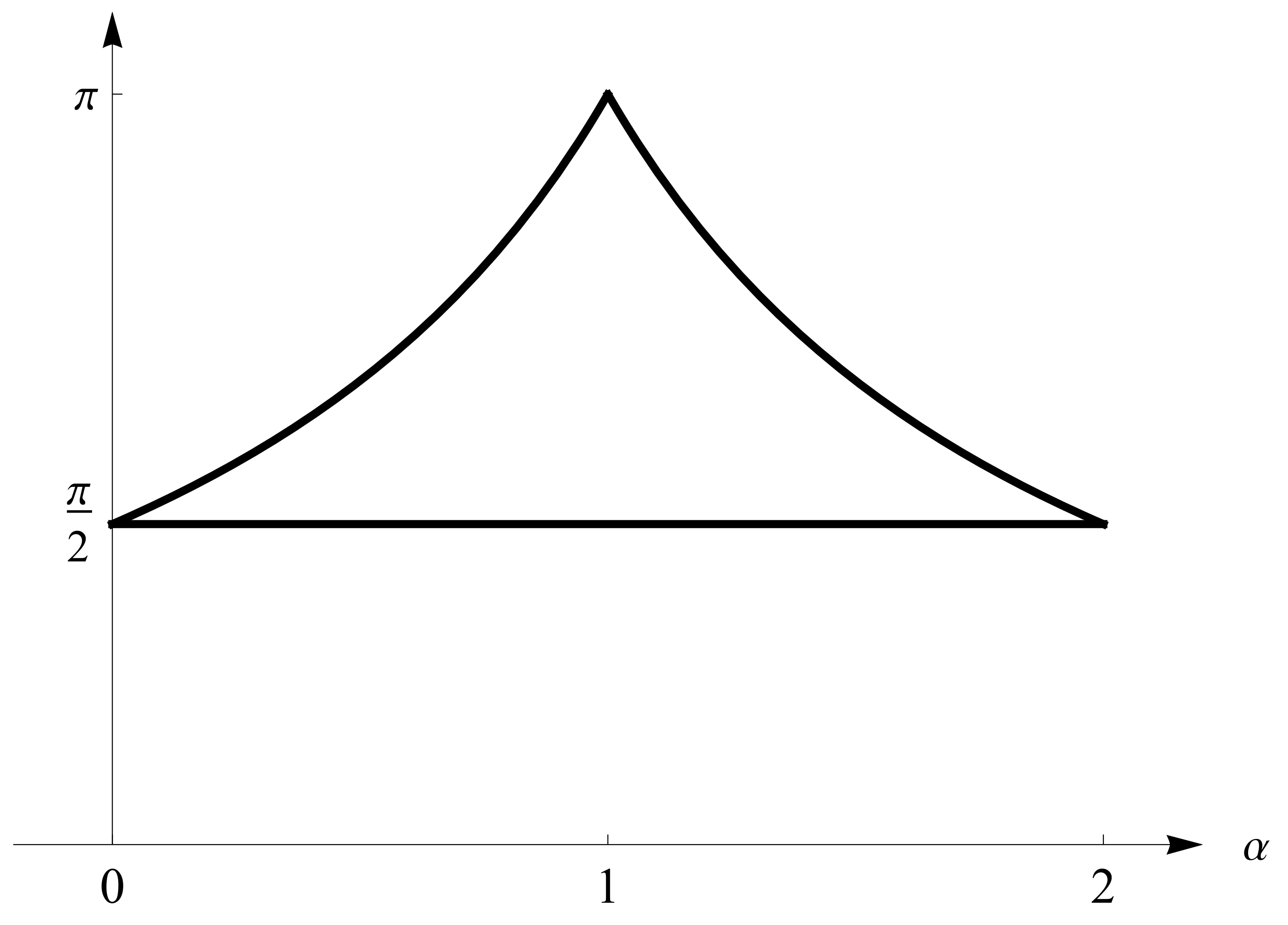
Here, the requirement $sin\left(\right(2-\alpha \left)\theta \right)>0$ is necessary, which implies the limitation for the argument

$$\mathrm{if}0<\alpha <1,\mathrm{then}\frac{\pi }{2}<\theta <\frac{\pi }{2-\alpha }.$$

(20)

The limitations for the argument in Equations (17) and (20) can be combined together as

$$\frac{\pi }{2}<\theta <\frac{\pi }{max\{\alpha ,2-\alpha \}},\alpha \in (0,1)\cup (1,2).$$

(21)

This range of limiting the argument of root is shown in Figure 1.

Figure 1. The range of argument of root limited by Equation (21).

Rewrite Equation (19) into the following form and define the left-hand side as the function $f(\theta ,\alpha )$,

$$\begin{array}{c}\hfill f(\theta ,\alpha ):=4b^{\frac{2}{2-\alpha }-2}{\left(\frac{{sin}^{\alpha }\left(\alpha \theta \right)}{{sin}^2\left(2\theta \right)}\right)}^{\frac{1}{2-\alpha }}sin\left((2-\alpha )\theta \right)=\frac{4c}{b^2}.\end{array}$$

(22)

Our aim is to show the argument $\theta$ of the root can be uniquely determined by Equation (22) for any specified $b>0$, $c>0$ and $\alpha \in (0,1)\cup (1,2)$. In Figure 2, surface $f(\theta ,\alpha )$ for $b=4$ is shown on the domain $0<\alpha <2$, $\frac{\pi }{2}<\theta <\frac{\pi }{max\{\alpha ,2-\alpha \}}$, where the vertical coordinates are limited in $0\le f(\theta ,\alpha )\le 5$.

Figure 2. Surface of $f(\theta ,\alpha )$ for $b=4$ on the domain: $0<\alpha <2$, $\frac{\pi }{2}<\theta <\frac{\pi }{max\{\alpha ,2-\alpha \}}$.

For fixed $\alpha$ and b, the function $f(\theta ,\alpha )$ satisfies the following limits,

$$\begin{array}{ccc}\hfill \underset{\theta \to {\left(\frac{\pi }{2}\right)}^{+}}{lim}f(\theta ,\alpha )=+\infty ,& & \mathrm{if}0<\alpha <1\mathrm{or}1<\alpha <2,\hfill \\ \hfill \underset{\theta \to {\left(\frac{\pi }{2-\alpha }\right)}^{-}}{lim}f(\theta ,\alpha )=0,& & \mathrm{if}0<\alpha <1,\hfill \\ \hfill \underset{\theta \to {\left(\frac{\pi }{\alpha }\right)}^{-}}{lim}f(\theta ,\alpha )=0,& & \mathrm{if}1<\alpha <2,\hfill \end{array}$$

as shown in Figure 2. Furthermore, the partial derivative with respect to $\theta$ is

$$\begin{array}{c}\hfill f_{\theta }^{\prime }(\theta ,\alpha )=\frac{4b^{-2}}{2-\alpha }{\left(\frac{b^2{sin}^{\alpha }\left(\alpha \theta \right)}{{sin}^2\left(2\theta \right)}\right)}^{\frac{1}{2-\alpha }}\frac{1}{sin\left(\alpha \theta \right)sin\left(2\theta \right)}g(\theta ,\alpha ),\end{array}$$

where

$$\begin{array}{c}\hfill g(\theta ,\alpha )=4{sin}^2\left(\alpha \theta \right)+{\alpha }^2{sin}^2\left(2\theta \right)-4\alpha sin\left(\alpha \theta \right)sin\left(2\theta \right)cos\left((2-\alpha )\theta \right),\end{array}$$

can be estimated as

$$\begin{array}{ccc}\hfill g(\theta ,\alpha )& >& 4{sin}^2\left(\alpha \theta \right)+{\alpha }^2{sin}^2\left(2\theta \right)+4\alpha sin\left(\alpha \theta \right)sin\left(2\theta \right)\hfill \\ & =& {(2sin\left(\alpha \theta \right)+\alpha sin\left(2\theta \right))}^2\ge 0.\hfill \end{array}$$

Because $sin\left(2\theta \right)<0$, so we have $f_{\theta }^{\prime }(\theta ,\alpha )<0.$

Thus, by the theorem of implicit function, for any $b>0$ and $c>0$, Equation (22) uniquely determines an implicit function of the argument of the root vs. $\alpha$, $\theta =\theta \left(\alpha \right),\alpha \in (0,1)\cup (1,2),$ which has the continuous derivative ${\theta }^{\prime }\left(\alpha \right)$. With the argument, the modulus of the root is determined from (18) as

$$\begin{array}{c}\hfill r=r\left(\alpha \right)={\left(\frac{bsin\left(\alpha \theta \right(\alpha \left)\right)}{-sin\left(2\theta \right(\alpha \left)\right)}\right)}^{\frac{1}{2-\alpha }},\alpha \in (0,1)\cup (1,2).\end{array}$$

(23)

We summarize the above deduction as follows, taking into account the conjugated part in the lower semi-complex plane.

Proposition 2.

For any $b>0$, $c>0$ and $\alpha \in (0,1)\cup (1,2)$, Equation (4) has exactly a pair of conjugated simple complex roots with a negative real part on the principal Riemann surface as $s\left(\alpha \right)=r\left(\alpha \right)e^{\mathrm{i}\theta \left(\alpha \right)}$ and $\overline{s}\left(\alpha \right)$, where $\theta \left(\alpha \right)$ satisfies the Equation (21) and is determined by Equation (22), and $r\left(\alpha \right)$ is determined by Equation (23).

The graphs of the implicit function $\theta =\theta \left(\alpha \right)$ determined by Equation (22) are shown in Figure 3 for $b=4$ and for $c=1$, 2, 4, 8 and 16. The outermost thin red dash curve is the boundary of $\theta$,

$$\theta =\frac{\pi }{max\{\alpha ,2-\alpha \}},$$

(24)

which corresponds to the limit $c\to 0^{+}$. The six curves arrayed outside-in from the outermost in Figure 3 are just the six level intersections of the surface in Figure 2 by the planes with the vertical coordinates 0, 0.25, 0.5, 1, 2 and 4.

Figure 3. Curves of $\theta \left(\alpha \right)$ vs. $\alpha$ for $b=4$ and for different values of c: $c=1$ (black dash line), 2 (purple dot-dash line), 4 (red solid line), 8 (blue dot line) and 16 (green dot-dot-dash line).

In Figure 3, dash line and dot-dash line are for the case of $b^2-4c>0$, solid line is for the case of $b^2-4c=0$ and dot line and dot-dot-dash line are for the case of $b^2-4c<0$. As $c\to 0^{+}$, the curve of $\theta \left(\alpha \right)$ approaches the boundary (24). We note that the left- and right-hand derivatives of the boundary (24) at $\alpha =1$ are

$${\theta }_{-}^{\prime }\left(1\right)=\pi ,{\theta }_{+}^{\prime }\left(1\right)=-\pi .$$

(25)

The function $r=r\left(\alpha \right)$ in Equation (23) is composed through the implicit function $\theta =\theta \left(\alpha \right)$. We note that the argument and the modulus of the root in the upper-half plane, $\theta \left(\alpha \right)$ and $r\left(\alpha \right)$, can be extended to define the closed interval $0\le \alpha \le 2$ by using the results of the integer cases in (5)–(9). That is, for $\alpha =0$ and 2, we have

$$\theta \left(0\right)=\theta \left(2\right)=\frac{\pi }{2},r\left(0\right)=\sqrt{c+b},r\left(2\right)=\sqrt{\frac{c}{1+b}},$$

while for $\alpha =1,$ we have

$$\begin{array}{lll}\mathrm{Case}1.& b^2-4c>0:& \theta \left(1\right)=\pi ,r_{1,2}\left(1\right)=\frac{b}{2}\pm \frac{\sqrt{b^2-4c}}{2},\hfill \end{array}$$

(26)

$$\begin{array}{lll}\mathrm{Case}2.& b^2-4c=0:& \theta \left(1\right)=\pi ,r\left(1\right)=\frac{b}{2},\hfill \end{array}$$

(27)

$$\begin{array}{lll}\mathrm{Case}3.& b^2-4c<0:& \theta \left(1\right)=arccos\left(-\frac{b}{2\sqrt{c}}\right),r\left(1\right)=\sqrt{c}.\hfill \end{array}$$

(28)

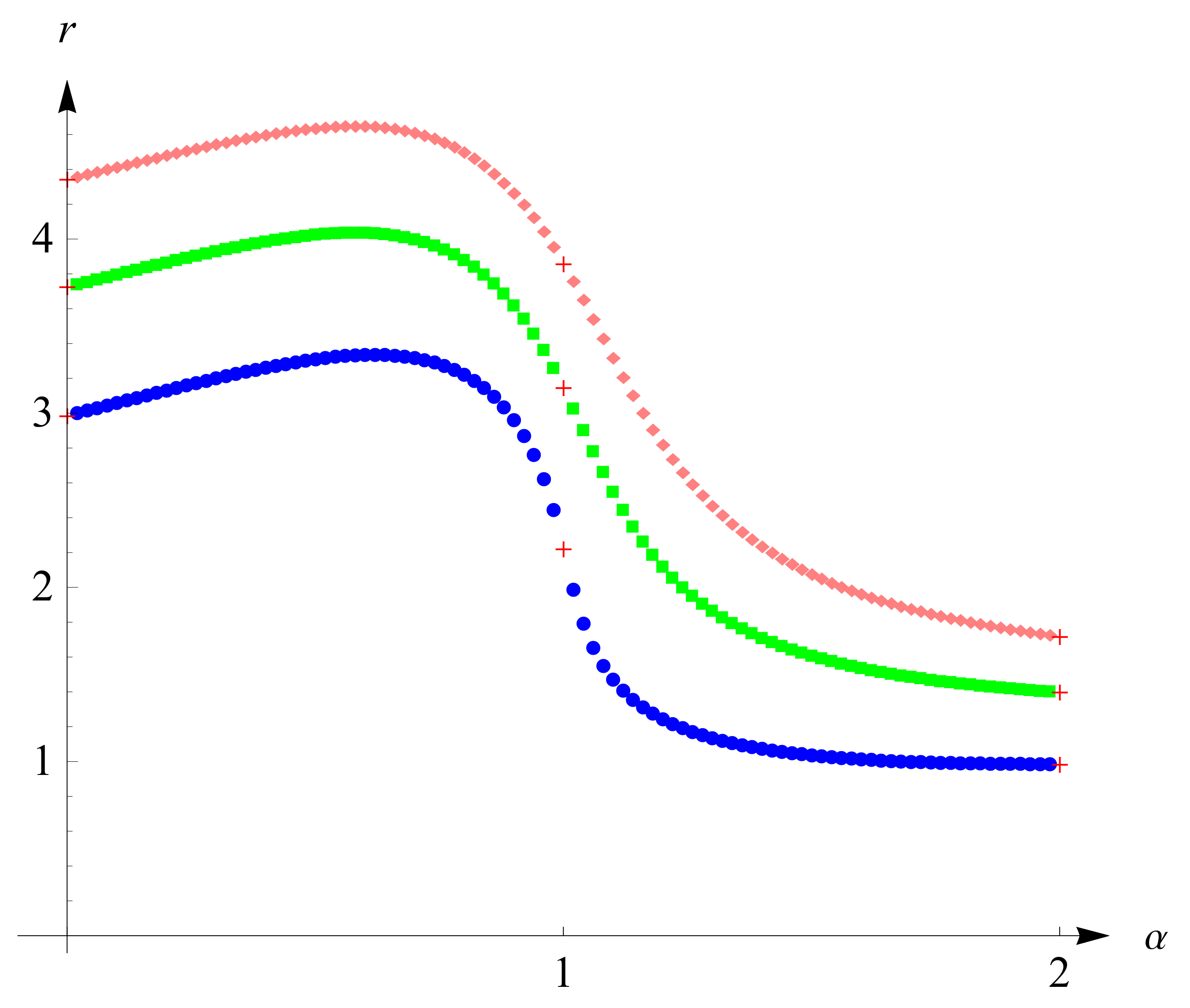
It is worth noting that for the case $\alpha =1$, $b^2-4c>0$, the moduli of roots are double-valued with $r_1\left(1\right)>r_2\left(1\right)$.

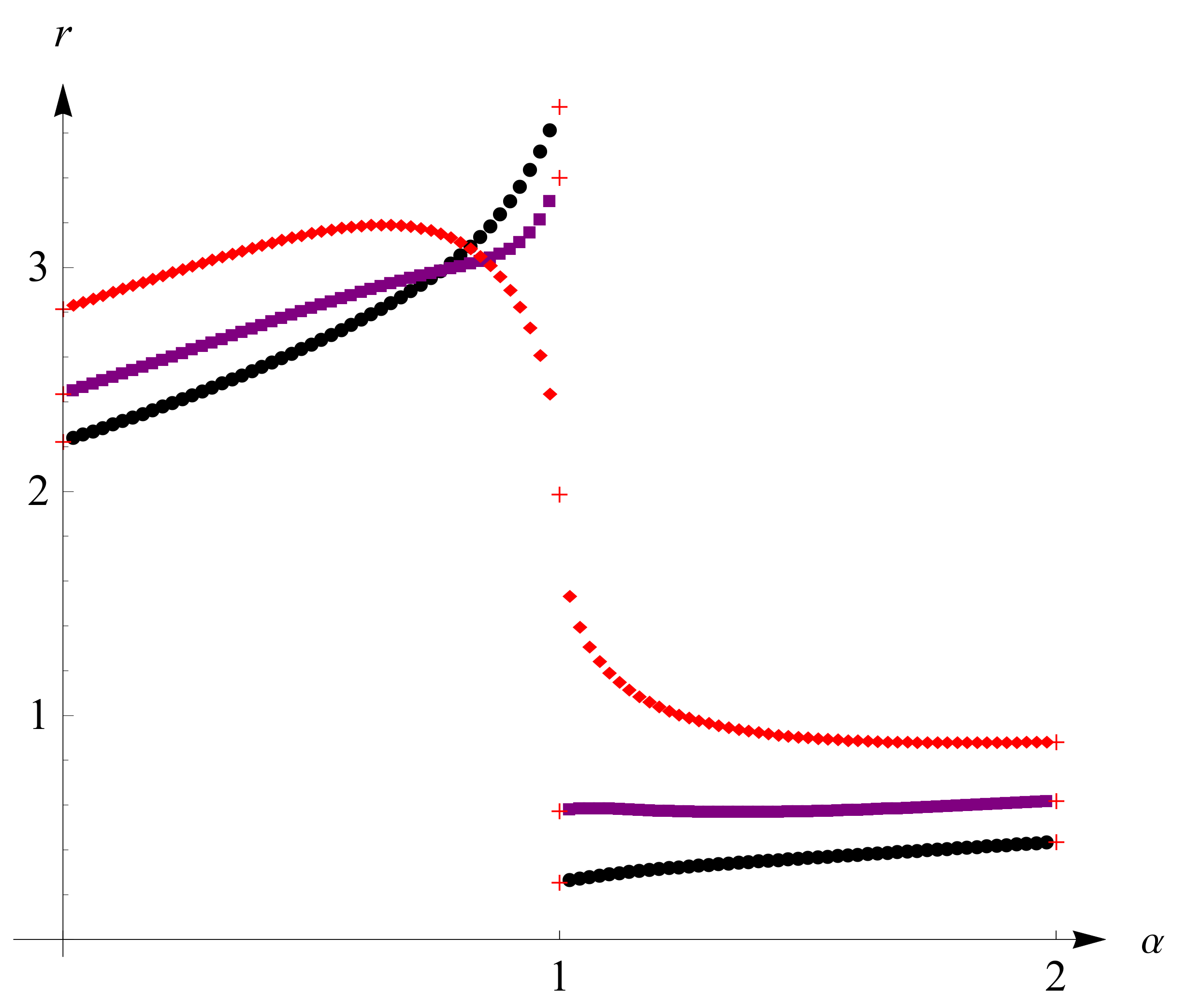
We depict the function $r=r\left(\alpha \right)$ on the discrete values of $\alpha$ with the step size 0.02:

$${\alpha }_j=0.02j,j=0,1,2,\cdots ,100.$$

(29)

The data plots are shown in Figure 4 for the cases of $b^2-4c>0$ and $b^2-4c=0$ and in Figure 5 for the case of $b^2-4c<0$, where data for the integer cases, $\alpha =0$, 1 and 2, are depicted by red ‘+’. We note that the circular dot line and square dot line in Figure 4 belong to the case $b^2-4c>0$, and jump discontinuities are shown at $\alpha =1$.

Figure 4. Curves of $r\left(\alpha \right)$ vs. $\alpha$ for $b=4$ and for $c=1$ (black circular dots), $c=2$ (purple square dots) and $c=4$ (red rhombic dots).

Figure 5. Curves of $r\left(\alpha \right)$ vs. $\alpha$ for $b=4$ and for $c=5$ (blue circular dots), $c=10$ (green square dots) and $c=15$ (pink rhombic dots).

For the two implicit functions $\theta \left(\alpha \right)$ and $r\left(\alpha \right)$, the derivatives can be given as follows. First, from (22) follows the partial derivative,

$$\begin{array}{c}\hfill f_{\alpha }^{\prime }(\theta ,\alpha )=\frac{4b^{-2}}{{(2-\alpha )}^2}{\left(\frac{b^2{sin}^{\alpha }\left(\alpha \theta \right)}{{sin}^2\left(2\theta \right)}\right)}^{\frac{1}{2-\alpha }}sin\left(\right(2-\alpha \left)\theta \right)h(\theta ,\alpha ),\end{array}$$

where

$$\begin{array}{c}\hfill h(\theta ,\alpha )=(2-\alpha )(\alpha cot\left(\alpha \theta \right)-(2-\alpha )cot\left((2-\alpha )\theta \right))\theta +ln\frac{b^2{sin}^2\left(\alpha \theta \right)}{{sin}^2\left(2\theta \right)}.\end{array}$$

By the formula of derivative of implicit function, we obtain

$$\begin{array}{c}\hfill {\theta }^{\prime }\left(\alpha \right)=-\frac{f_{\alpha }^{\prime }(\theta ,\alpha )}{f_{\theta }^{\prime }(\theta ,\alpha )}=-\frac{sin\left(\alpha \theta \right)sin\left(2\theta \right)sin\left(\right(2-\alpha \left)\theta \right)h(\theta ,\alpha )}{(2-\alpha )g(\theta ,\alpha )},\end{array}$$

(30)

and furthermore, from Equation (23), we derive

$$\begin{array}{c}\hfill r^{\prime }\left(\alpha \right)=\frac{r\left(\alpha \right)}{2-\alpha }\left[\theta cot\left(\alpha \theta \right)+{\theta }^{\prime }\left(\alpha \right)(\alpha cot\left(\alpha \theta \right)-2cot\left(2\theta \right))+ln\left(r\left(\alpha \right)\right)\right].\end{array}$$

(31)

Note that in Equations (30) and (31), $\theta$ denotes the implicit function $\theta \left(\alpha \right)$. The two derivatives will be used in the next section.

Proposition 3.

Suppose $0<\alpha <1$, then $s=r{e}^{\mathrm{i}\theta }$ is a root of equation $s^2+b{s}^{\alpha }+c=0$ if and only if $s=\frac{1}{r}{e}^{\mathrm{i}\theta }$ is a root of equation

$$s^2+\frac{b}{c}{s}^{2-\alpha }+\frac{1}{c}=0.$$

(32)

Proof. 

If $s=r{e}^{\mathrm{i}\theta }$ is a root of equation $s^2+b{s}^{\alpha }+c=0$, then $r^2{e}^{\mathrm{i}2\theta }+b{r}^{\alpha }{e}^{\mathrm{i}\alpha \theta }+c=0$, which is equivalent to its conjugate $r^2{e}^{-\mathrm{i}2\theta }+b{r}^{\alpha }{e}^{-\mathrm{i}\alpha \theta }+c=0$. Then, multiplied by $\frac{1}{c{r}^2}{e}^{\mathrm{i}2\theta }$ on the two sides, the equation becomes

$$\frac{1}{r^2}{e}^{\mathrm{i}2\theta }+\frac{b}{c}\frac{1}{r^{2-\alpha }}{e}^{\mathrm{i}(2-\alpha )\theta }+\frac{1}{c}=0.$$

This means $s=\frac{1}{r}{e}^{\mathrm{i}\theta }$ is a root of Equation (32). The reverse is also true. The proof is completed. □

From Figure 3, the curve of $\theta \left(\alpha \right)$ is not symmetrical about the straight line $\alpha =1$ in general. However, from Proposition 3, a sufficient condition for symmetry can be given as follows.

Proposition 4.

Suppose the argument of the root of equation $s^2+b{s}^{\alpha }+1=0$ on the upper-half complex plane is $\theta \left(\alpha \right)$, where $0\le \alpha \le 2$, then the function $\theta \left(\alpha \right)$ satisfies the equality $\theta \left(\alpha \right)=\theta (2-\alpha )$, i.e., the curve of $\theta \left(\alpha \right)$ vs. α is symmetrical about the straight line $\alpha =1$.

3. Root Trajectories in Three Cases

In this section, we consider the variation of the root $s\left(\alpha \right)=r\left(\alpha \right)e^{\mathrm{i}\theta \left(\alpha \right)}$ with respect to $\alpha$ in three cases clarified by the discriminant $b^2-4c$. Our discussion concentrates upon the upper-half complex plane and is based on the fact that the argument of the root, $\theta \left(\alpha \right)$, is continuous on the interval $0\le \alpha \le 2$. Special attention is paid to the variation of the root $s\left(\alpha \right)$ near $\alpha =1$.

Case 1. $b^2-4c>0$

In this case, the limit of the argument of the root is $\underset{\alpha \to 1}{lim}\theta \left(\alpha \right)=\theta \left(1\right)=\pi ,$ which is the peak value of $\theta \left(\alpha \right)$. For the modulus in Equation (23), by L’Hospital rule

$$\begin{array}{c}\hfill \underset{\alpha \to 1^{-}}{lim}r\left(\alpha \right)=\underset{\alpha \to 1^{-}}{lim}\frac{bsin\left(\alpha \theta \right(\alpha \left)\right)}{-sin\left(2\theta \right(\alpha \left)\right)}=\frac{b}{2}\underset{\alpha \to 1^{-}}{lim}\left(\alpha +\frac{\theta }{{\theta }^{\prime }\left(\alpha \right)}\right)=\frac{b}{2}\left(1+\frac{\pi }{{\theta }_{-}^{\prime }\left(1\right)}\right).\end{array}$$

(33)

Similarly,

$$\begin{array}{c}\hfill \underset{\alpha \to 1^{+}}{lim}r\left(\alpha \right)=\frac{b}{2}\left(1+\frac{\pi }{{\theta }_{+}^{\prime }\left(1\right)}\right).\end{array}$$

(34)

Due to that $\theta \left(1\right)$ is the maximum value of $\theta \left(\alpha \right)$, so ${\theta }_{-}^{\prime }\left(1\right)\ge 0$ and ${\theta }_{+}^{\prime }\left(1\right)\le 0$. Thus, from Equations (33) and (34), we have $\underset{\alpha \to 1^{-}}{lim}r\left(\alpha \right)\ge \underset{\alpha \to 1^{+}}{lim}r\left(\alpha \right).$ The two limits should equal the absolute values of the two unequal real roots of the case $\alpha =1$ in Equation (7), i.e., the following equations hold,

$$\begin{array}{c}\hfill \underset{\alpha \to 1^{-}}{lim}r\left(\alpha \right)=\frac{b+\sqrt{b^2-4c}}{2},\underset{\alpha \to 1^{+}}{lim}r\left(\alpha \right)=\frac{b-\sqrt{b^2-4c}}{2}.\end{array}$$

(35)

Thus, $r\left(\alpha \right)$ has a downward jump when $\alpha$ increasingly passes through 1, as shown in Figure 4. Substituting the two limits into Equations (33) and (34), we obtain

$$\begin{array}{c}\hfill {\theta }_{-}^{\prime }\left(1\right)=\frac{b\pi }{\sqrt{b^2-4c}},{\theta }_{+}^{\prime }\left(1\right)=-\frac{b\pi }{\sqrt{b^2-4c}}.\end{array}$$

(36)

The limit case of $c\to 0^{+}$ is consistent with the boundary in Equation (25). Therefore, for the root $s\left(\alpha \right)=r\left(\alpha \right)e^{\mathrm{i}\theta \left(\alpha \right)}$, we have the following result.

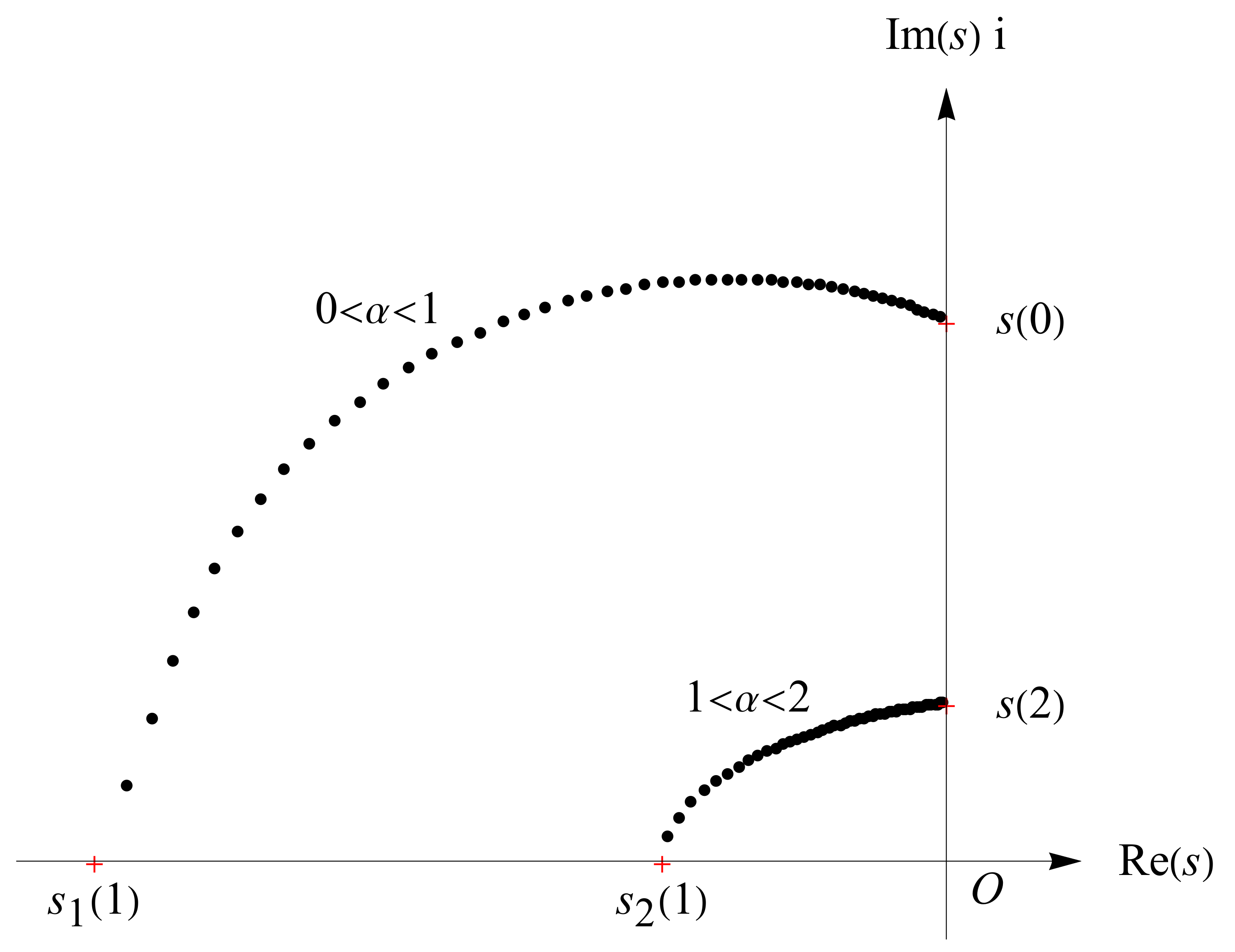
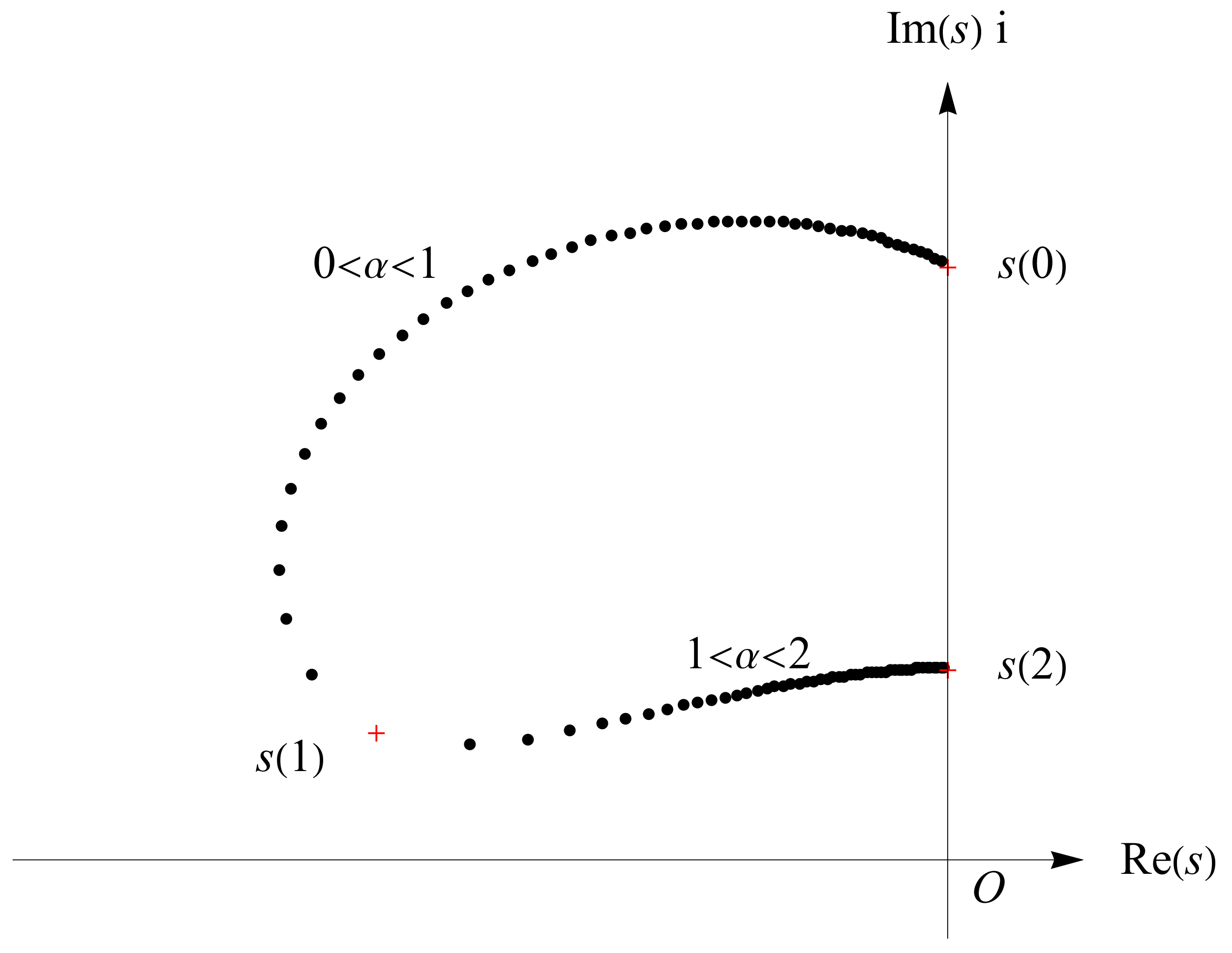
Proposition 5.

If $b^2-4c>0$, then in the upper-half complex plane, the root $s\left(\alpha \right)$ as a function of α is discontinuous at $\alpha =1$, and

$$\begin{array}{c}\hfill \underset{\alpha \to 1^{-}}{lim}s\left(\alpha \right)=s_1\left(1\right)=-\frac{b+\sqrt{b^2-4c}}{2},\end{array}$$

(37)

$$\begin{array}{c}\hfill \underset{\alpha \to 1^{+}}{lim}s\left(\alpha \right)=s_2\left(1\right)=-\frac{b-\sqrt{b^2-4c}}{2}.\end{array}$$

(38)

Taking $b=4$, $c=3$ and $\alpha$ as the values in Equation (29), the trajectory of roots $s\left(\alpha \right)$ in the upper-half complex plane is shown in Figure 6, where $s\left(0\right)=\sqrt{7}\mathrm{i}$, $s\left(2\right)=\sqrt{0.6}\mathrm{i}$, $s_1\left(1\right)=-3$ and $s_2\left(1\right)=-1$, indicated in red crosses, are the roots for the integer cases $\alpha =0$, 2 and 1 in the upper-half complex plane.

Figure 6. Trajectory of roots $s\left(\alpha \right)$ for $\alpha$ varying between 0 and 2, where $b=4$ and $c=3$ $(b^2-4c>0)$.

Case 2. $b^2-4c=0$

For the critical case, the argument of the root satisfies the limit $\underset{\alpha \to 1}{lim}\theta \left(\alpha \right)=\theta \left(1\right)=\pi .$ As a limiting case of $b^2-4c\to 0^{+}$, from Equations (35) and (36), we have

$$\begin{array}{c}\hfill \underset{\alpha \to 1}{lim}r\left(\alpha \right)=\frac{b}{2},{\theta }_{-}^{\prime }\left(1\right)=+\infty ,{\theta }_{+}^{\prime }\left(1\right)=-\infty .\end{array}$$

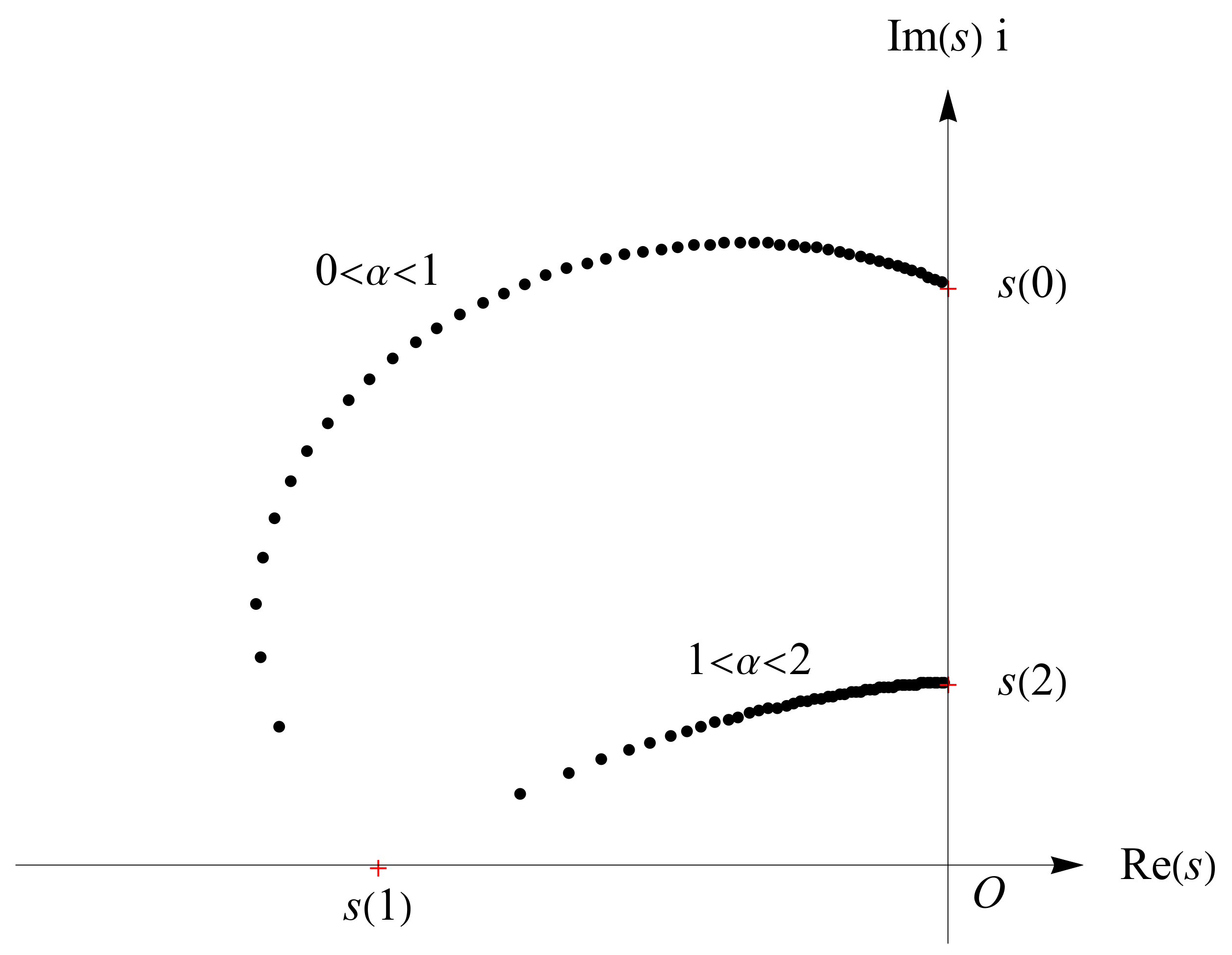
Therefore, the root $s\left(\alpha \right)$ is continuous at $\alpha =1$, but non-differentiable at $\alpha =1$.

Taking $b=4$, $c=4$ and $\alpha$ as the values in Equation (29), the trajectory of roots $s\left(\alpha \right)$ in the upper-half complex plane is shown in Figure 7, where $s\left(0\right)=2\sqrt{2}\mathrm{i}$, $s\left(2\right)=\sqrt{0.8}\mathrm{i}$ and $s\left(1\right)=-2$, indicated in red crosses, are the roots for the integer cases $\alpha =0$, 2 and 1 in the upper-half complex plane.

Figure 7. Trajectory of roots $s\left(\alpha \right)$ for $\alpha$ varying between 0 and 2, where $b=4$ and $c=4$ $(b^2-4c=0)$.

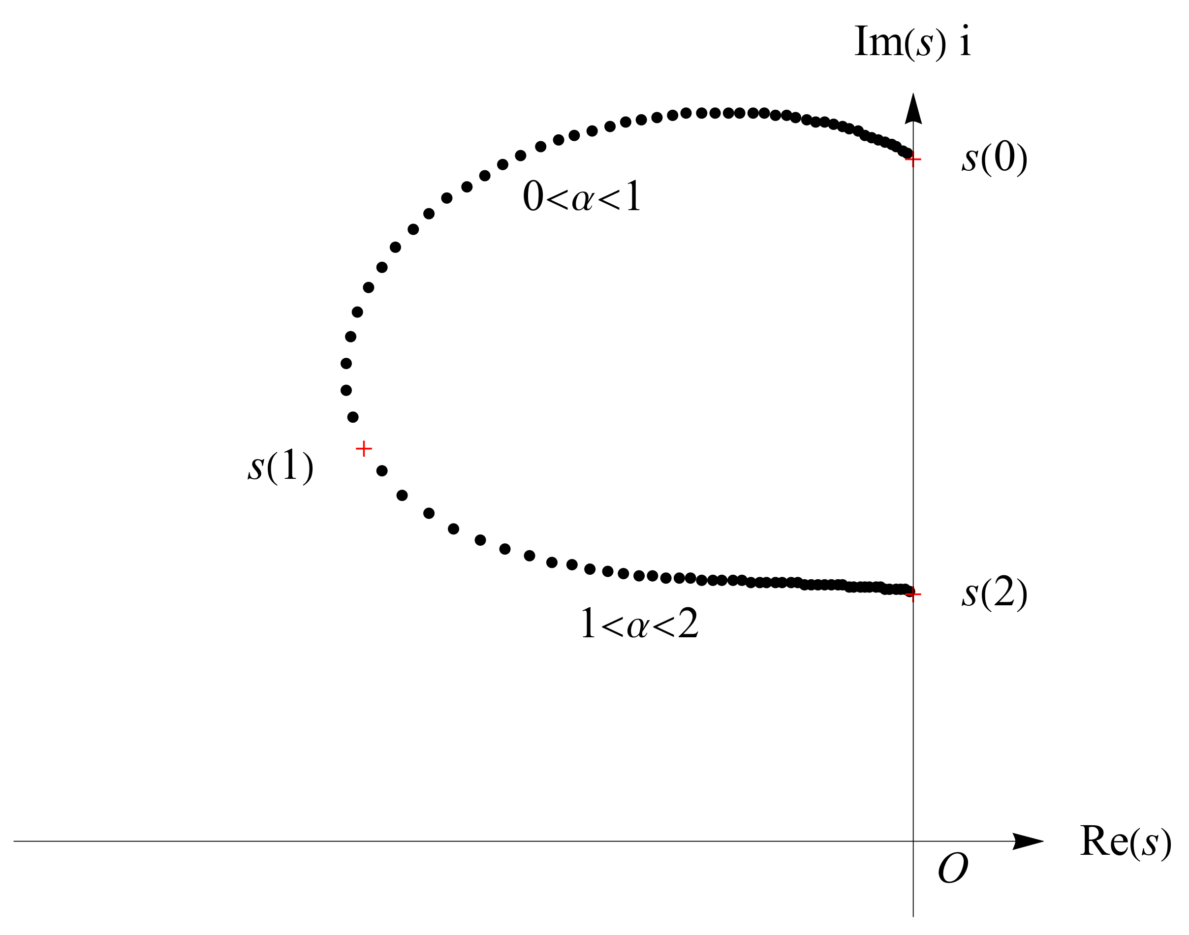
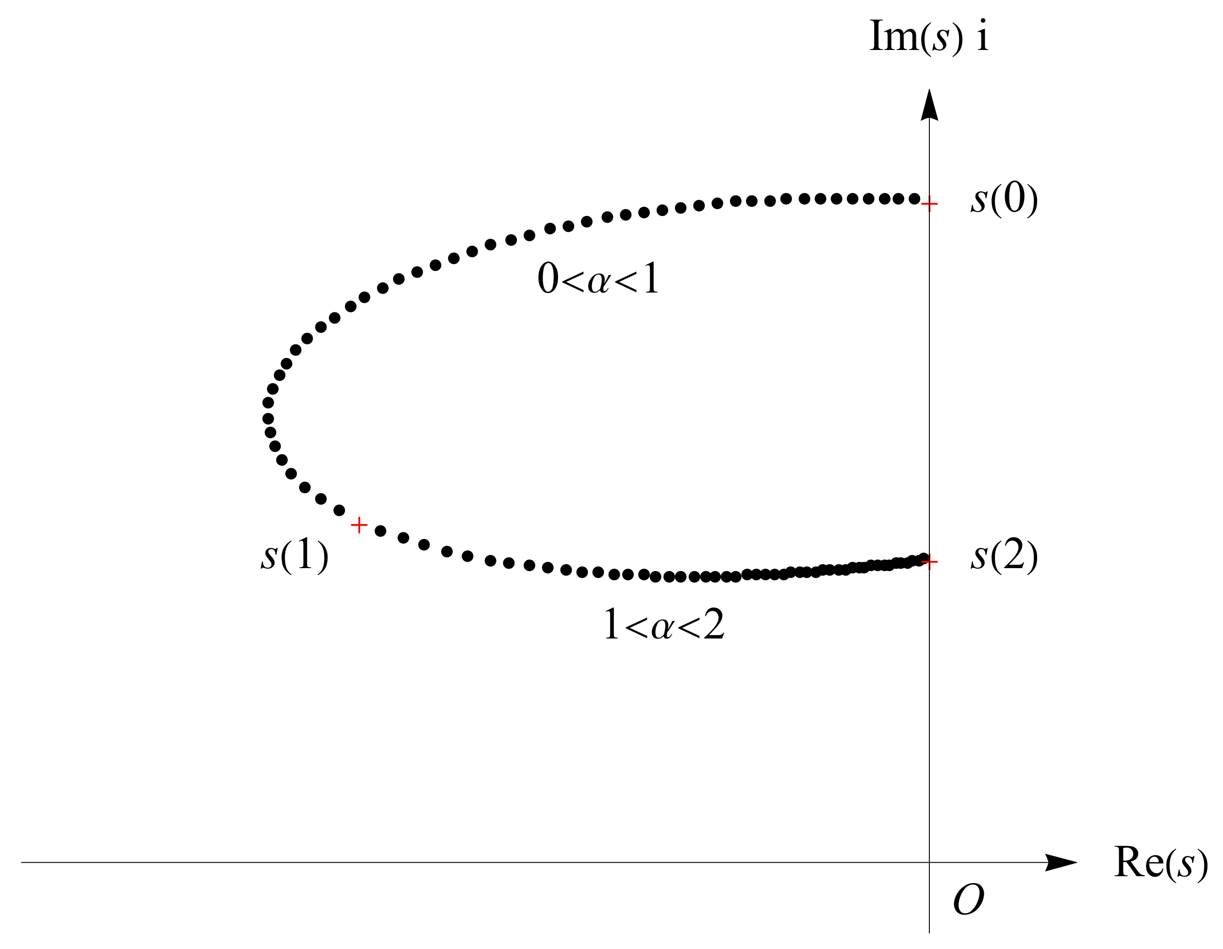
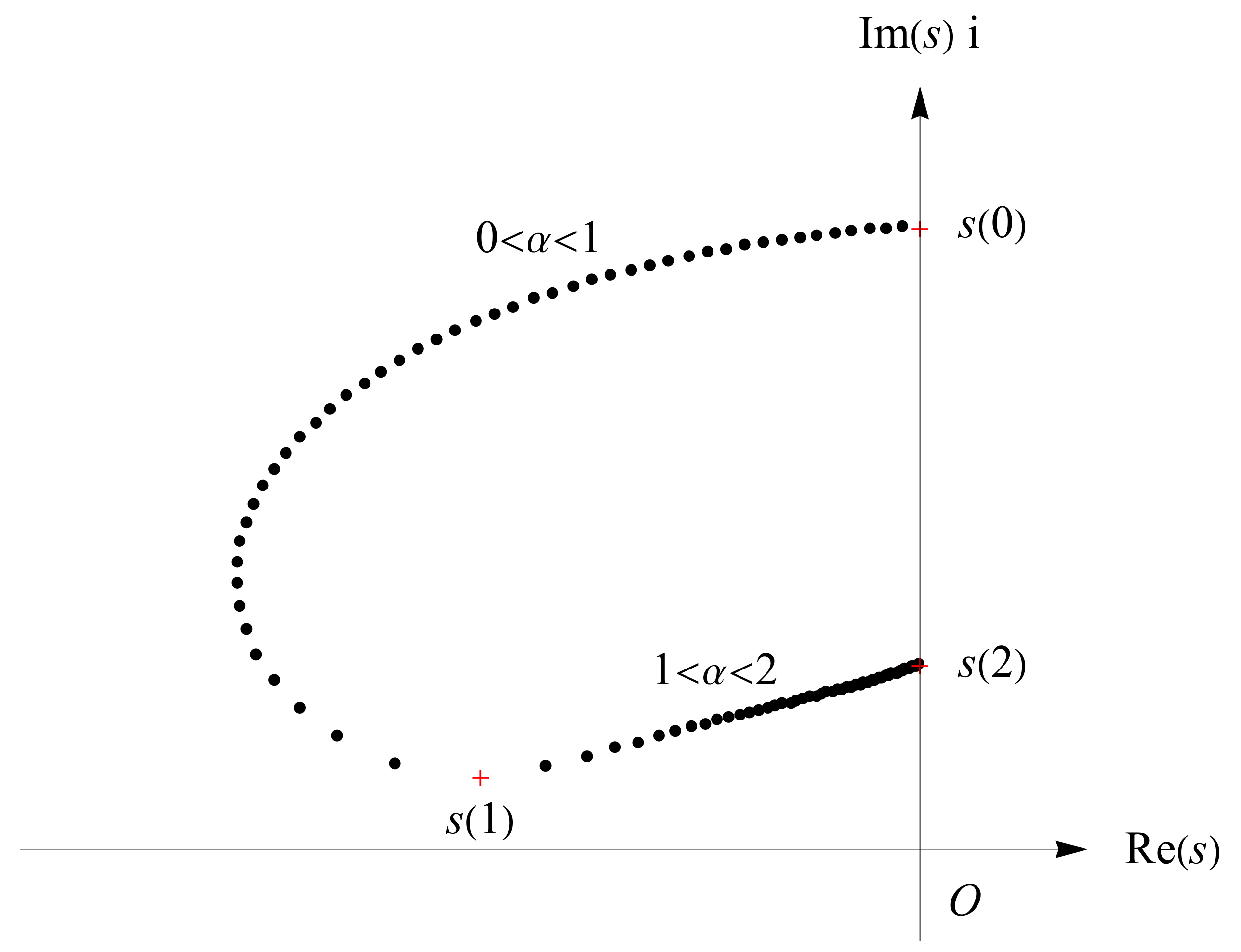
Case 3. $b^2-4c<0$

In this case, from Equation (28), the argument and modulus of the root in the upper-half complex plane have the limits $\underset{\alpha \to 1}{lim}\theta \left(\alpha \right)=\theta \left(1\right)=arccos\left(-\frac{b}{2\sqrt{c}}\right)$ and $\underset{\alpha \to 1}{lim}r\left(\alpha \right)=r\left(1\right)=\sqrt{c}.$ The root $s\left(\alpha \right)$ is continuous at $\alpha =1$, and also differentiable, which will be further discussed in the next section.

Taking $b=4$, $c=4.4$ and $\alpha$ as the values in Equation (29), where $-b<b^2-4c<0$, the trajectory of roots $s\left(\alpha \right)$ is shown in Figure 8, where $s\left(0\right)=\sqrt{8.4}\mathrm{i}$, $s\left(2\right)=\sqrt{0.88}\mathrm{i}$ and $s\left(1\right)=-2+\sqrt{0.4}\mathrm{i}$, indicated in red crosses, are the roots for the integer cases $\alpha =0$, 2 and 1 in the upper-half complex plane. As a comparison, we take $b=4$ and $c=8$ satisfying $b^2-4c<-b$, and the trajectory of roots $s\left(\alpha \right)$ is shown in Figure 9, where $s\left(0\right)=2\sqrt{3}\mathrm{i}$, $s\left(2\right)=\sqrt{1.6}\mathrm{i}$ and $s\left(1\right)=-2+2\mathrm{i}$ are indicated in red crosses and are the roots for the integer cases $\alpha =0$, 2 and 1 in the upper-half complex plane. Note that for comparison purposes, scale ranges of the horizontal and vertical axes in Figure 6, Figure 7, Figure 8 and Figure 9 are consistent.

Figure 8. Trajectory of roots $s\left(\alpha \right)$ for $\alpha$ varying between 0 and 2, where $b=4$ and $c=4.4$ $(-b<b^2-4c<0)$.

Figure 9. Trajectory of roots $s\left(\alpha \right)$ for $\alpha$ varying between 0 and 2, where $b=4$ and $c=8$ $(b^2-4c<-b)$.

From the trajectories of roots, $s\left(\alpha \right)$ has a faster change rate as $\alpha$ approaches 1. For the cases of $b^2-4c\ge 0$, the imaginary part of the root $s\left(\alpha \right)$ can become arbitrarily small as $\alpha$ approaches 1. For the case of $b^2-4c<0$, the smaller the value $b^2-4c$, the larger the imaginary part of the root $s\left(1\right)$.

4. Further Discussion for the Case of ${\mathbf{b}}^{\mathbf{2}}-\mathbf{4}\mathbf{c}<\mathbf{0}$

From the last section, we know that the root trajectory $s\left(\alpha \right)$ has better behavior at $\alpha =1$ in the case of $b^2-4c<0$ than other cases. We confine to the case $b^2-4c<0$ and further clarify the variation of roots $s\left(\alpha \right)$ according to the change rates of the argument $\theta \left(\alpha \right)$, real part $\lambda \left(\alpha \right)$ and imaginary part $\omega \left(\alpha \right)$ of roots $s\left(\alpha \right)$ at $\alpha =1$. The discussion is confined to the upper-half complex plane.

From Equations (28) and (30), we derive that

$${\theta }^{\prime }\left(1\right)=\frac{blnc}{2\sqrt{4c-b^2}},$$

(39)

and further, from Equations (28), (31) and (39), we obtain

$$r^{\prime }\left(1\right)=-\frac{b\sqrt{c}}{\sqrt{4c-b^2}}arccos\left(-\frac{b}{2\sqrt{c}}\right).$$

(40)

It is apparent that $r^{\prime }\left(1\right)<0$ is always true. That is, the modulus of root, $r\left(\alpha \right)$, decreases invariably at $\alpha =1$. From Equation (39), if $c=1$, then ${\theta }^{\prime }\left(1\right)=0$, and if $c<1$, then ${\theta }^{\prime }\left(1\right)<0$, while if $c>1$, then ${\theta }^{\prime }\left(1\right)>0$.

Now, consider the real part and the imaginary part of the root

$$\begin{array}{c}\hfill \lambda \left(\alpha \right)=\mathrm{Re}\left(s\right(\alpha \left)\right)=r\left(\alpha \right)cos\left(\theta \right(\alpha \left)\right),\omega \left(\alpha \right)=\mathrm{Im}\left(s\right(\alpha \left)\right)=r\left(\alpha \right)sin\left(\theta \right(\alpha \left)\right),\end{array}$$

and its derivative

$$\begin{array}{ccc}& & {\lambda }^{\prime }\left(\alpha \right)=r^{\prime }\left(\alpha \right)cos\left(\theta \left(\alpha \right)\right)-r\left(\alpha \right)sin\left(\theta \left(\alpha \right)\right){\theta }^{\prime }\left(\alpha \right),\hfill \end{array}$$

(41)

$$\begin{array}{ccc}& & {\omega }^{\prime }\left(\alpha \right)=r^{\prime }\left(\alpha \right)sin\left(\theta \left(\alpha \right)\right)+r\left(\alpha \right)cos\left(\theta \left(\alpha \right)\right){\theta }^{\prime }\left(\alpha \right).\hfill \end{array}$$

(42)

Substituting Equations (28), (39) and (40) into Equation (41), we acquire the derivative of the real part at $\alpha =1$ as a function of b and c,

$${\lambda }^{\prime }\left(1\right)={\lambda }^{\prime }(1;b,c)=p(b,c):=\frac{b^2}{2\sqrt{4c-b^2}}arccos\left(-\frac{b}{2\sqrt{c}}\right)-\frac{blnc}{4}.$$

(43)

Proposition 6.

The equation $p(b,c)=0$ uniquely determines a continuous and monotonically increasing implicit function $c=\xi \left(b\right)$ defined on the interval $0<b<+\infty$ such that $\xi \left(b\right)>b^2/4$ and $\xi \left(0^{+}\right)=1$. The curve $L_1$ of the implicit function $c=\xi \left(b\right)$ divides the domain $b^2-4c<0$ in the $(b,c)$ plane into two regions, and ${\lambda }^{\prime }\left(1\right)<0$ above the curve $L_1$ and ${\lambda }^{\prime }\left(1\right)>0$ below the curve $L_1$.

Proof. 

For any fixed $b>0$, the limits hold

$$\begin{array}{c}\hfill \underset{c\to +\infty }{lim}p(b,c)=-\infty ,\underset{c\to {\left(\frac{b^2}{4}\right)}^{+}}{lim}p(b,c)=+\infty .\end{array}$$

Further, the partial derivative is calculated from (43) as

$$\begin{array}{c}\hfill p_c^{\prime }(b,c)=-\frac{b^2}{{(4c-b^2)}^{3/2}}arccos\left(-\frac{b}{2\sqrt{c}}\right)-\frac{b}{4c-b^2}<0.\end{array}$$

Thus, the equation $p(b,c)=0$ uniquely determines a continuous implicit function $c=\xi \left(b\right)$ defined on $0<b<+\infty$ such that $\xi \left(b\right)>b^2/4$.

Calculating the partial derivative with respect to b, we have

$$\begin{array}{c}\hfill p_b^{\prime }(b,c)=\frac{b^2}{2(4c-b^2)}-\frac{1}{4}lnc+\frac{b(8c-b^2)}{2{(4c-b^2)}^{3/2}}arccos\left(-\frac{b}{2\sqrt{c}}\right).\end{array}$$

(44)

It follows from the equation $p(b,c)=0$ that

$$lnc=\frac{2b}{\sqrt{4c-b^2}}arccos\left(-\frac{b}{2\sqrt{c}}\right).$$

(45)

Replacing $lnc$ in Equation (44) by using Equation (45), we obtain

$$\begin{array}{c}\hfill p_b^{\prime }(b,c)=\frac{b^2}{2(4c-b^2)}+\frac{2bc}{{(4c-b^2)}^{3/2}}arccos\left(-\frac{b}{2\sqrt{c}}\right)>0.\end{array}$$

Hence, the derivative of the implicit function $c=\xi \left(b\right)$ is

$$\begin{array}{c}\hfill {\xi }^{\prime }\left(b\right)=-\frac{p_b^{\prime }(b,c)}{p_c^{\prime }(b,c)}>0.\end{array}$$

Therefore, the implicit function $c=\xi \left(b\right)$ is monotonically increasing. Finally, by letting $b\to 0^{+}$ in Equation (45), we obtain $\xi \left(0^{+}\right)=1$. Thus, the curve $L_1$ of the implicit function $c=\xi \left(b\right)$ divides the domain $b^2-4c<0$ in the $(b,c)$ plane into two regions. The signs of ${\lambda }^{\prime }\left(1\right)$ are deduced from the equation ${\lambda }^{\prime }\left(1\right)=p(b,c).$ The proof is completed. □

For the derivative of the imaginary part at $\alpha =1$, from Equations (28), (39), (40) and (42), we have

$$\begin{array}{c}\hfill {\omega }^{\prime }\left(1\right)={\omega }^{\prime }(1;b,c):=q(b,c)=-\frac{b}{2}arccos\left(-\frac{b}{2\sqrt{c}}\right)-\frac{b^{2}lnc}{4\sqrt{4c-b^2}}.\end{array}$$

(46)

Proposition 7.

The equation $q(b,c)=0$ uniquely determines a continuous and monotonically increasing implicit function $c=\zeta \left(b\right)$ defined on the interval $0<b<2$ such that $b^2/4<\zeta \left(b\right)<1$ and $\zeta \left(0^{+}\right)=0$, $\zeta \left(2^{-}\right)=1$. The curve $L_2$ of the implicit function $c=\zeta \left(b\right)$ divides the domain $b^2-4c<0$ in the $(b,c)$ plane into two regions, and ${\omega }^{\prime }\left(1\right)<0$ above the curve $L_2$ and ${\omega }^{\prime }\left(1\right)>0$ below the curve $L_2$.

Proof. 

In the domain $b^2-4c<0$, if $c\ge 1$, then ${\omega }^{\prime }\left(1\right)<0$ from Equation (46). Now, we look into the function $q(b,c)$ in the region $0<b<2,b^2/4<c<1.$ For any fixed b$(0<b<2)$, the limits hold

$$\begin{array}{c}\hfill \underset{c\to {\left(\frac{b^2}{4}\right)}^{+}}{lim}q(b,c)=+\infty ,\underset{c\to 1^{-}}{lim}q(b,c)=-\frac{b}{2}arccos\left(-\frac{b}{2}\right)<0.\end{array}$$

Calculating the partial derivatives, we have

$$\begin{array}{ccc}& & q_c^{\prime }(b,c)=\frac{b^{2}lnc}{2{(4c-b^2)}^{3/2}}<0,\hfill \\ & & q_b^{\prime }(b,c)=\frac{2c}{4c-b^2}arccos\left(-\frac{b}{2\sqrt{c}}\right)-\frac{b}{2\sqrt{4c-b^2}},\hfill \end{array}$$

where the equation $q(b,c)=0$ is used. Now, we estimate the second partial derivative as follows,

$$\begin{array}{c}\hfill q_b^{\prime }(b,c)\ge \frac{2\pi c-b\sqrt{4c-b^2}}{2(4c-b^2)}.\end{array}$$

Moreover, from the inequality $4{\pi }^2{c}^2>4c(4c-b^2)>b^2(4c-b^2)>0$, we deduce that $q_b^{\prime }(b,c)>0.$ Therefore, the equation $q(b,c)=0$ uniquely determines a continuous and monotonically increasing implicit function $c=\zeta \left(b\right)$ defined on the interval $0<b<2$ such that $b^2/4<\zeta \left(b\right)<1$, and from Equation (46), we know that $\zeta \left(0^{+}\right)=0$ and $\zeta \left(2^{-}\right)=1$. Thus, the curve $L_2$ of the implicit function $c=\zeta \left(b\right)$ divides the domain $b^2-4c<0$ in the $(b,c)$ plane into two regions. The signs of ${\omega }^{\prime }\left(1\right)$ are deduced from the equation ${\omega }^{\prime }\left(1\right)=q(b,c).$ The proof is completed. □

From the above analyses, the curves $L_1$, $c=1$ and $L_2$ subdivide the domain $b^2-4c<0$ in the $(b,c)$ plane into four disjoint regions, as shown in Figure 10. The region IV is narrow and is magnified in Figure 11. The characteristics of the four regions in the domain $b^2-4c<0$ are listed in Table 1.

Figure 10. Curves of $b^2-4c=0$ (solid line), $c=1$ (dot line), $p(b,c)=0$ (dash line) and $q(b,c)=0$ (red dot-dash line).

Figure 11. Local zoom of the rectangular area $0\le b\le 2$, $0\le c\le 1$ in Figure 10.

Table 1. Characteristics of four regions in the domain $b^2-4c<0$.

Regions	Constraint Conditions	Characteristics of Roots at $\mathit{\alpha }=1$	Samples ($\mathit{b},\mathit{c})$ and Root Trajectories
I	$p(b,c)<0$	${\theta }^{\prime }\left(1\right)>0$, ${\lambda }^{\prime }\left(1\right)<0$, ${\omega }^{\prime }\left(1\right)<0$	$(3,15)$; Figure 12
II	$p(b,c)>0,$$c>1$	${\theta }^{\prime }\left(1\right)>0$, ${\lambda }^{\prime }\left(1\right)>0$, ${\omega }^{\prime }\left(1\right)<0$	$(4,4.4)$ and $(4,8)$; Figure 8 and Figure 9
III	$c<1$, $q(b,c)<0$	${\theta }^{\prime }\left(1\right)<0$, ${\lambda }^{\prime }\left(1\right)>0$, ${\omega }^{\prime }\left(1\right)<0$	$(0.9,0.6)$; Figure 13
IV	$q(b,c)>0$	${\theta }^{\prime }\left(1\right)<0$, ${\lambda }^{\prime }\left(1\right)>0$, ${\omega }^{\prime }\left(1\right)>0$	$(0.6,0.1)$; Figure 14

In region I, we take a sample $b=3$, $c=15$ and depict the trajectory of roots $s\left(\alpha \right)$ in Figure 12. In Figure 8, $b=4$, $c=4.4$, and in Figure 9, $b=4$, $c=8$, which are all in region II. In region III, we take a sample $b=0.9$, $c=0.6$, and the trajectory of roots is shown in Figure 13. In region IV, we take $b=0.6$, $c=0.1$ and display the trajectory of roots in Figure 14.

Figure 12. Trajectory of roots $s\left(\alpha \right)$ for $\alpha$ varying between 0 and 2, where $b=3$ and $c=15$ $(b^2-4c<0$, region I).

Figure 13. Trajectory of roots $s\left(\alpha \right)$ for $\alpha$ varying between 0 and 2, where $b=0.9$ and $c=0.6$ $(b^2-4c<0$, region III).

Figure 14. Trajectory of roots $s\left(\alpha \right)$ for $\alpha$ varying between 0 and 2, where $b=0.6$ and $c=0.1$ $(b^2-4c<0$, region IV).

Note that region IV is in the immediate vicinity of the critical case $b^2-4c=0$. This means that only when $s\left(1\right)$ is close enough to the real axis, its imaginary part may satisfy ${\omega }^{\prime }\left(1\right)>0$.

5. The Residue Contribution and Hankel Integral Contribution to the Impulsive Response

Consider the noninteger case $\alpha \in (0,1)\cup (1,2)$, and denote the couple of conjugated complex roots of the characteristic Equation (4) on the principal Riemann surface as $s\left(\alpha \right)=r\left(\alpha \right)e^{\mathrm{i}\theta \left(\alpha \right)}=\lambda \left(\alpha \right)+\mathrm{i}\omega \left(\alpha \right)$ and $\overline{s}\left(\alpha \right)$, where $\lambda \left(\alpha \right)<0$ and $\omega \left(\alpha \right)>0$. By the residue theorem, the solution in Equation (3) can be decomposed into two components: the residue contribution and the Hankel integral contribution,

$$z(t;\alpha )=z_R(t;\alpha )+z_H(t;\alpha ),$$

(47)

where

$$\begin{array}{ccc}\hfill z_R(t;\alpha )& =& \mathrm{Res}\left[\frac{e^{st}}{s^2+b{s}^{\alpha }+c},s\left(\alpha \right)\right]+\mathrm{Res}\left[\frac{e^{st}}{s^2+b{s}^{\alpha }+c},\overline{s}\left(\alpha \right)\right],\hfill \end{array}$$

(48)

$$\begin{array}{ccc}\hfill z_H(t;\alpha )& =& \frac{1}{2\pi \mathrm{i}}{\int }_{\mathrm{Ha}}\frac{e^{st}}{s^2+b{s}^{\alpha }+c}ds.\hfill \end{array}$$

(49)

We note that the Hankel path, Ha, is a loop starting from $-\infty$ and going along the lower side of the negative real axis to the origin O, encircling the origin counterclockwise with the radius approaching 0 and passing through the upper side of the negative real axis and ending at $-\infty$. Calculating the residues in Equation (48), we obtain the residue contribution

$$z_R(t;\alpha )=2e^{\lambda \left(\alpha \right)t}\frac{Psin\left(\omega \right(\alpha \left)t\right)+Qcos\left(\omega \right(\alpha \left)t\right)}{P^2+Q^2},$$

(50)

where

$$\begin{array}{ccc}& & P=2r\left(\alpha \right)sin\left(\theta \left(\alpha \right)\right)+b\alpha {\left(r\left(\alpha \right)\right)}^{\alpha -1}sin\left(\left(\alpha -1\right)\theta \left(\alpha \right)\right),\hfill \\ & & Q=2r\left(\alpha \right)cos\left(\theta \left(\alpha \right)\right)+b\alpha {\left(r\left(\alpha \right)\right)}^{\alpha -1}cos\left(\left(\alpha -1\right)\theta \left(\alpha \right)\right).\hfill \end{array}$$

The Hankel integral in Equation (49) is reduced to the following real infinite integral

$$\begin{array}{c}\hfill z_H(t;\alpha )=\frac{1}{\pi }{\int }_0^{+\infty }K(\rho ,\alpha )e^{-\rho t}d\rho ,\end{array}$$

(51)

where

$$\begin{array}{c}\hfill K(\rho ,\alpha )=\frac{b{\rho }^{\alpha }sin\left(\pi \alpha \right)}{{({\rho }^2+c+b{\rho }^{\alpha }cos\left(\pi \alpha \right))}^2+{(b{\rho }^{\alpha }sin\left(\pi \alpha \right))}^2}.\end{array}$$

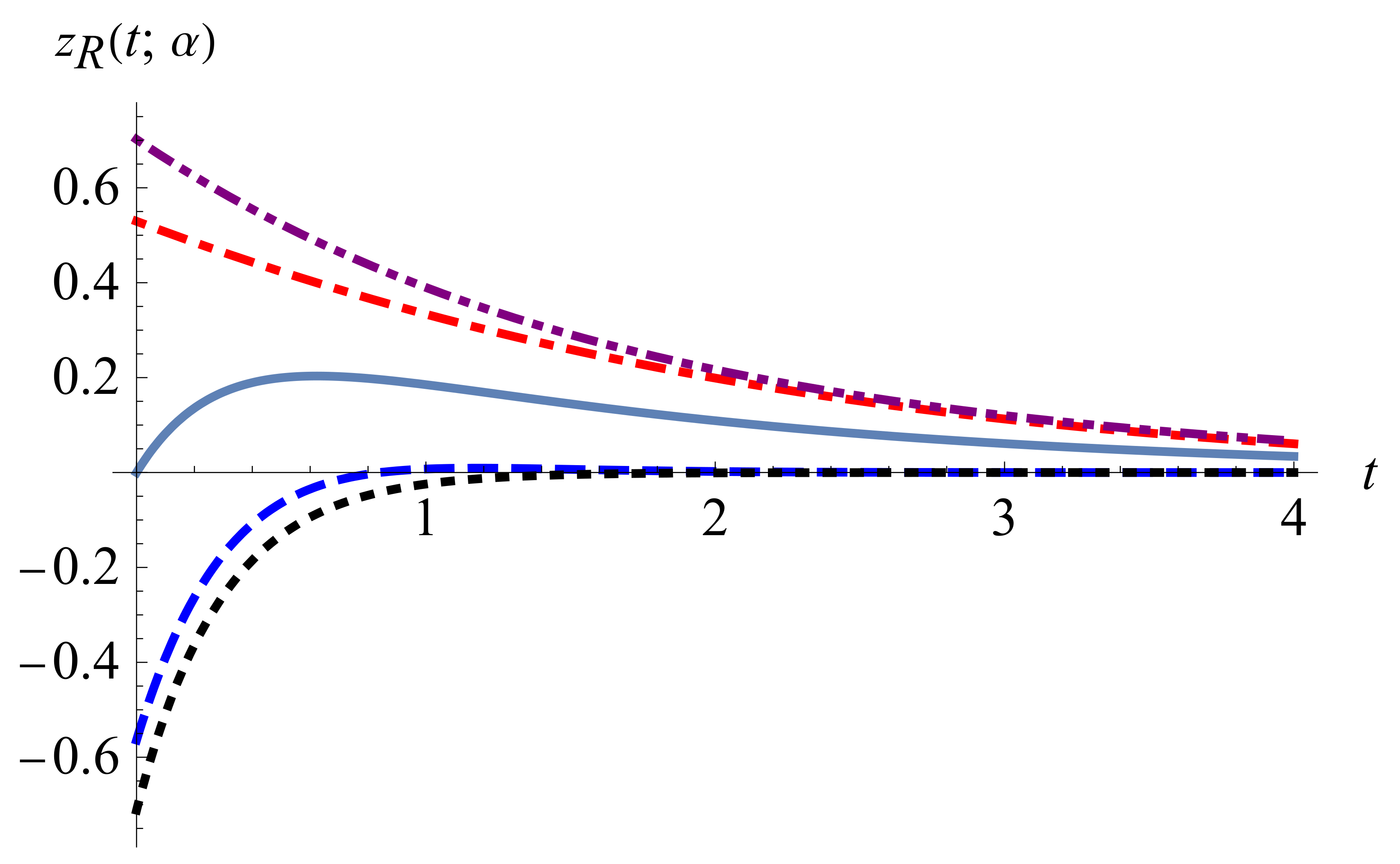
It seems that the residue contribution $z_R(t;\alpha )$ approaches $z(t;1)$ in Equations (12)–(14) and the Hankel integral contribution $z_H(t;\alpha )$ approaches 0 as $\alpha \to 1.$ However, the facts are not so and depend on the sign of the discriminant $b^2-4c$. If $b^2-4c>0$, then from Equations (37) and (50), the left-hand limit of the residue contribution $z_R(t;\alpha )$ at $\alpha =1$ is

$$z_R(t;1^{-})=-\frac{2}{\sqrt{b^2-4c}}{e}^{-\frac{b+\sqrt{b^2-4c}}{2}t},$$

while from Equations (38) and (50), the right-hand limit of $z_R(t;\alpha )$ at $\alpha =1$ is

$$z_R(t;1^{+})=\frac{2}{\sqrt{b^2-4c}}{e}^{-\frac{b-\sqrt{b^2-4c}}{2}t}.$$

The two limits produce a jump, neither equals $z(t;1)$ in Equations (12) and they satisfy the relationship $z(t;1)=(z_R(t;1^{-})+z_R(t;1^{+}))/2$. In fact, the Hankel integral contribution $z_H(t;\alpha )$ does not vanish as $\alpha \to 1$ but fills up the jump such that $z(t;\alpha )\to z(t;1)$ as $\alpha \to 1$. This can be seen from Figure 15 and Figure 16. If $b^2-4c=0$, then the variations of $z_R(t;\alpha )$ and $z_H(t;\alpha )$ are similar to the former case, see Figure 17 and Figure 18.

Figure 15. Curves of $z(t;1)$ (solid line) and residue contribution $z_R(t;\alpha )$ for $\alpha =$ 0.9 (dash line), 0.99 (dot line), 1.1 (dot-dash line), 1.01 (dot-dot-dash line), where $b=4$ and $c=2$ $(b^2-4c>0$).

Figure 16. Curves of $z(t;1)$ (solid line) and $z(t;\alpha )$ for $\alpha =$ 0.9 (dash line), 0.99 (dot line), 1.1 (dot-dash line), 1.01 (dot-dot-dash line), where $b=4$ and $c=2$ $(b^2-4c>0$).

Figure 17. Curves of $z(t;1)$ (solid line) and residue contribution $z_R(t;\alpha )$ for $\alpha =$ 0.9 (dash line), 0.99 (dot line), 1.1 (dot-dash line), 1.01 (dot-dot-dash line), where $b=4$ and $c=4$ $(b^2-4c=0$).

Figure 18. Curves of $z(t;1)$ (solid line) and residue contribution $z(t;\alpha )$ for $\alpha =$ 0.9 (dash line), 0.99 (dot line), 1.1 (dot-dash line), 1.01 (dot-dot-dash line), where $b=4$ and $c=4$ $(b^2-4c=0$).

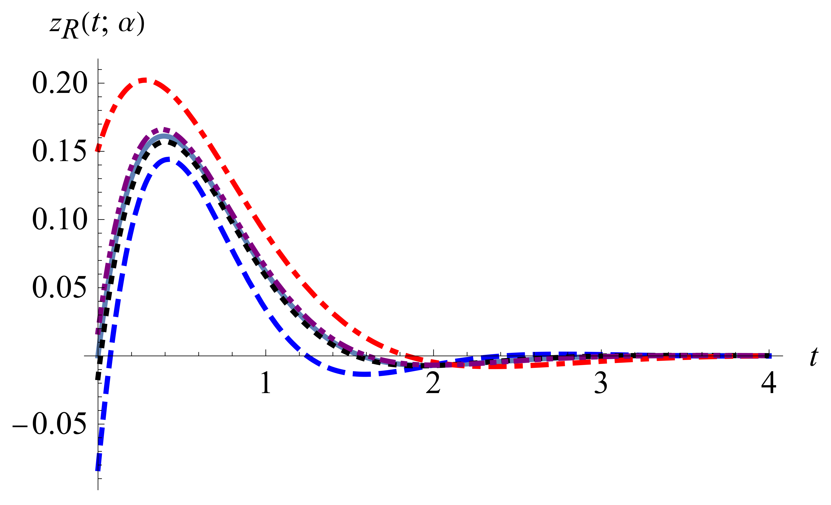
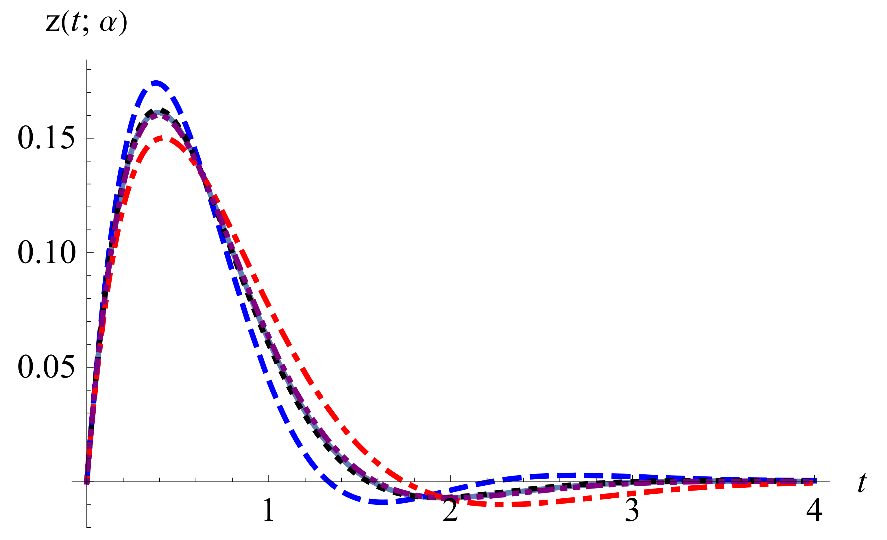
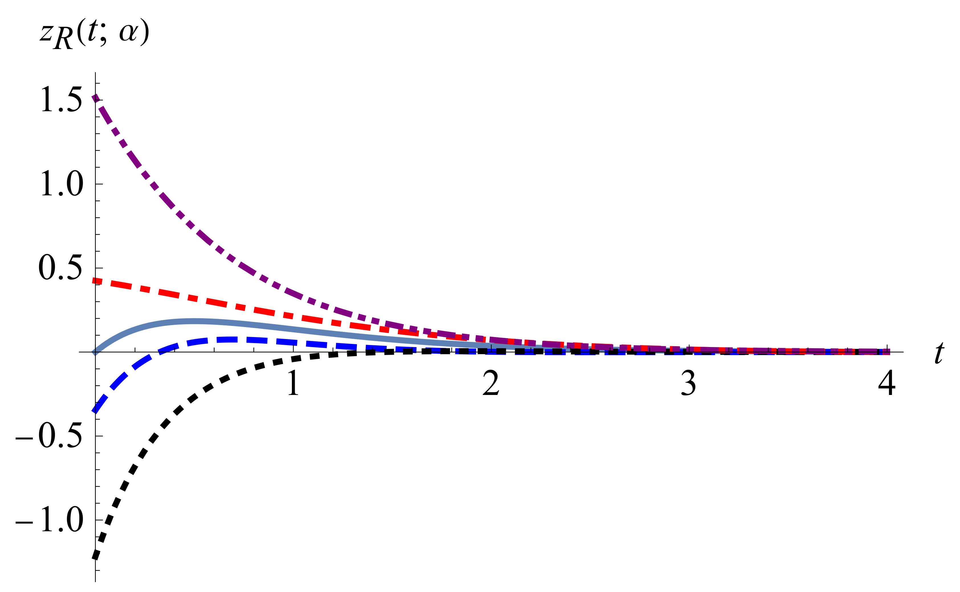
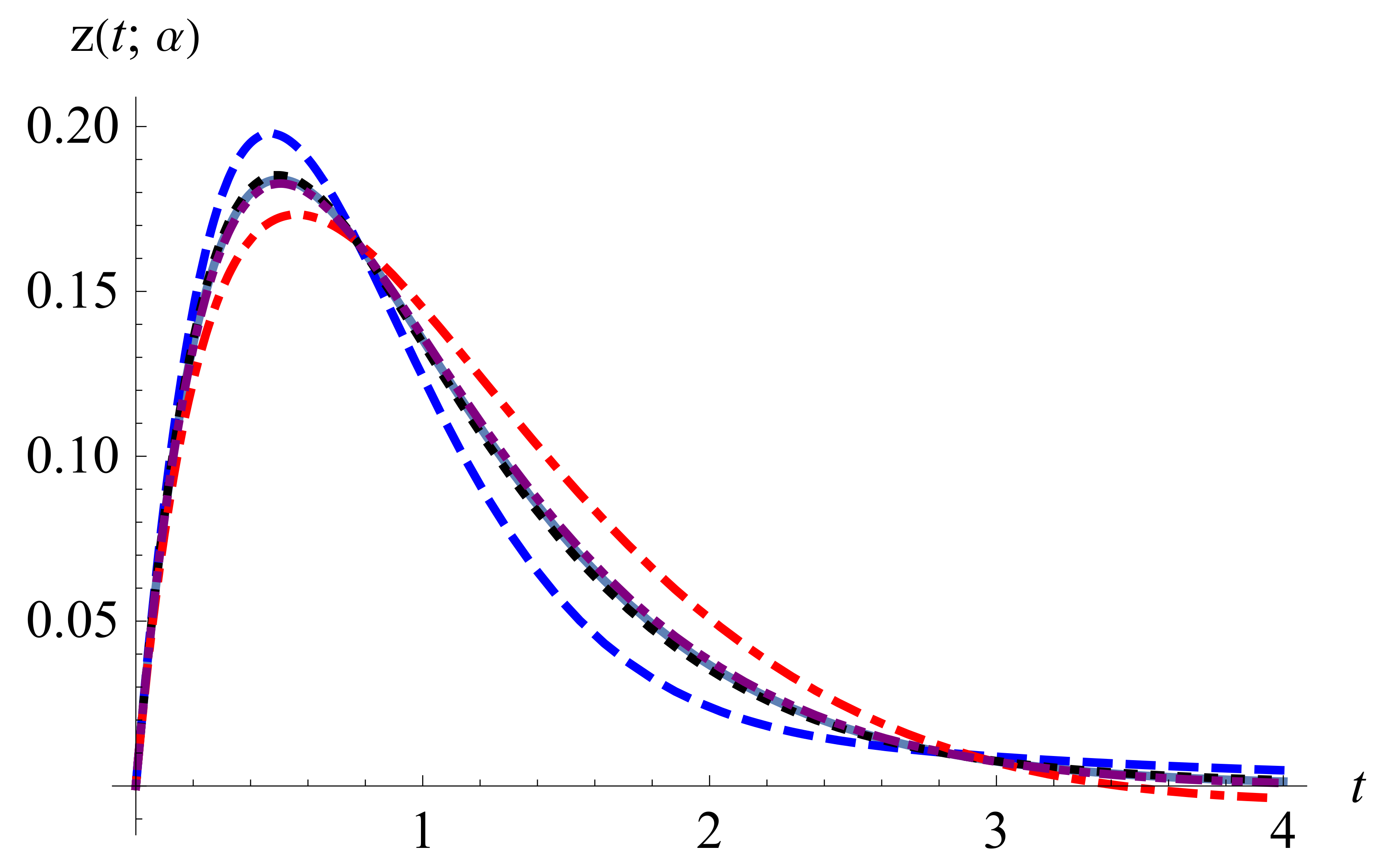
Nevertheless, if $b^2-4c<0$, then the variations of the residue contribution $z_R(t;\alpha )$ and the Hankel integral contribution $z_H(t;\alpha )$ are different from the former two situations. From Equations (9), (28) and (50), we derive that $z_R(t;\alpha )\to z(t;1)$ in Equation (14) as $\alpha \to 1.$ Moreover, from Figure 19 and Figure 20, we can see that the residue contribution $z_R(t;\alpha )$ approaches $z(t;1)$ and the Hankel integral contribution $z_H(t;\alpha )$ approaches 0 as $\alpha \to 1$.

Figure 19. Curves of $z(t;1)$ (solid line) and residue contribution $z_R(t;\alpha )$ for $\alpha =$ 0.9 (dash line), 0.99 (dot line), 1.1 (dot-dash line), 1.01 (dot-dot-dash line), where $b=4$ and $c=8$ $(b^2-4c<0$).

Figure 20. Curves of $z(t;1)$ (solid line) and $z(t;\alpha )$ for $\alpha =$ 0.9 (dash line), 0.99 (dot line), 1.1 (dot-dash line), 1.01 (dot-dot-dash line), where $b=4$ and $c=8$ $(b^2-4c<0$).

6. Conclusions

We consider the roots of the characteristic Equation (4) of the fractional vibration Equation (1) on the principal Riemann surface for the three cases of the discriminant $b^2-4c$: $>0$, $=0$ and $<0$, and with the range of $\alpha$ covering the interval $0\le \alpha \le 2$. Particular attention is paid to the varying of the roots $s\left(\alpha \right)$ as a function of the order $\alpha$ near $\alpha =1$ on the upper-half complex plane. We find that the root trajectories of the characteristic equation with $\alpha$ varying have different behaviors in the three cases of the discriminant. The residue contribution and Hankel integral contribution serve as two solution components of the impulsive response of the fractional vibration equation. It is found that the changing pattern of the solution components as $\alpha \to 1$ depends on the sign of the discriminant $b^2-4c$.

In Section 2, we prove that for any $b>0$, $c>0$ and $\alpha \in (0,1)\cup (1,2)$, the characteristic Equation (4) has a pair of conjugated simple complex roots with a negative real part. For the three cases of the discriminant $b^2-4c$, the variations of the argument and modulus of the roots according to $\alpha$ are clarified. For the integer-order cases, $\alpha =0$, 1 and 2, the inverse Laplace transform gives the known analytic results. In Section 3, the trajectories of the roots $s\left(\alpha \right)$ on the upper-half complex plane are analyzed and simulated for the three cases of the discriminant $b^2-4c$. For the case of $b^2-4c>0$, the root $s\left(\alpha \right)$ as a function of $\alpha$ is discontinuous at $\alpha =1$, and the left and right limits equal the two different real roots of the case $\alpha =1$ as in Equations (37) and (38). For the case of $b^2-4c=0$, the root $s\left(\alpha \right)$ is continuous at $\alpha =1$ but non-differentiable at $\alpha =1$. For the case of $b^2-4c<0$, the root $s\left(\alpha \right)$ is continuous and also differentiable at $\alpha =1$. In Section 4, the particular analyses for the case of $b^2-4c<0$ are conducted. The trajectories of the roots $s\left(\alpha \right)$ are further clarified in the domain $b^2-4c<0$ on the $(b,c)$ plane according to the change rates of the argument $\theta \left(\alpha \right)$, real part $\lambda \left(\alpha \right)$ and imaginary part $\omega \left(\alpha \right)$ of the root $s\left(\alpha \right)$ at $\alpha =1$. For this purpose, the domain $b^2-4c<0$ is subdivided into four disjoint regions to clarify the trajectories of the roots.

In Section 5, the residue contribution and Hankel integral contribution to the impulsive response of the fractional vibration equation are considered. For the cases of $b^2-4c\ge 0$, the left and right limits of the residue contribution $z_R(t;\alpha )$ at $\alpha =1$ produce a jump and neither equals $z(t;1)$. The Hankel integral contribution $z_H(t;\alpha )$ does not vanish as $\alpha \to 1$ but fills up the jump such that $z(t;\alpha )=z_R(t;\alpha )+z_H(t;\alpha )\to z(t;1)$ as $\alpha \to 1$. Nevertheless, for the case of $b^2-4c<0$, the variations of $z_R(t;\alpha )$ and $z_H(t;\alpha )$ are different from the cases $b^2-4c\ge 0$, and we derive that the residue contribution $z_R(t;\alpha )$ approaches $z(t;1)$ as $\alpha \to 1,$ and so the Hankel integral contribution $z_H(t;\alpha )$ approaches 0 as $\alpha \to 1$.

For the two solution components in Equations (50) and (51), the residue contribution represents a damping oscillation, while the Hankel integral contribution provides a monotonic recovering. Moreover, asymptotic behaviors can be obtained conveniently from the solution components [23]. In the residue contribution (50), the real part $\lambda \left(\alpha \right)$ and imaginary part $\omega \left(\alpha \right)$ of the root $s\left(\alpha \right)$ describe the decaying rate of the amplitude and the oscillation frequency, respectively. These results could be helpful for revealing the relationship between the model parameters b, c and $\alpha$ and the oscillation properties. Finally, we indicate that there are few reports on the root trajectories of an equation with a fractional power.