Article

Finite Iterative Forecasting Model Based on Fractional Generalized Pareto Motion

1
School of Electronic and Electrical Engineering, Minnan University of Science and Technology, Quanzhou 362700, China
2
Key Laboratory of Industrial Automation Control Technology and Application of Fujian Higher Education, Quanzhou 362700, China
3
School of Electronic & Electrical Engineering, Shanghai University of Science Engineering, Shanghai 201620, China
4
Jiangxi New Energy Technology Institute, Xinyu 338000, China
5
MINES Paris, PSL University, CRC, 06904 Sophia Antipolis, France
6
Energy Department, Politecnico di Milano, Via La Masa 34/3, 20156 Milan, Italy
*
Author to whom correspondence should be addressed.
Fractal Fract. 2022, 6(9), 471; https://doi.org/10.3390/fractalfract6090471
Submission received: 9 July 2022 / Revised: 5 August 2022 / Accepted: 22 August 2022 / Published: 26 August 2022
(This article belongs to the Special Issue New Trends in Fractional Stochastic Processes)

Abstract

:
In this paper, an efficient prediction model based on the fractional generalized Pareto motion (fGPm) with Long-Range Dependent (LRD) and infinite variance characteristics is proposed. Firstly, we discuss the meaning of each parameter of the generalized Pareto distribution (GPD), and the LRD characteristics of the generalized Pareto motion are analyzed by taking into account the heavy-tailed characteristics of its distribution. Then, the mathematical relationship H = 1 α between the self-similar parameter H and the tail parameter α is obtained. Also, the generalized Pareto increment distribution is obtained using statistical methods, which offers the subsequent derivation of the iterative forecasting model based on the increment form. Secondly, the tail parameter α is introduced to generalize the integral expression of the fractional Brownian motion, and the integral expression of fGPm is obtained. Then, by discretizing the integral expression of fGPm, the statistical characteristics of infinite variance is shown. In addition, in order to study the LRD prediction characteristic of fGPm, LRD and self-similarity analysis are performed on fGPm, and the LRD prediction conditions H > 1 α is obtained. Compared to the fractional Brownian motion describing LRD by a self-similar parameter H , fGPm introduces the tail parameter α , which increases the flexibility of the LRD description. However, the two parameters are not independent, because of the LRD condition H > 1 α . An iterative prediction model is obtained from the Langevin-type stochastic differential equation driven by fGPm. The prediction model inherits the LRD condition H > 1 α of fGPm and the time series, simulated by the Monte Carlo method, shows the superiority of the prediction model to predict data with high jumps. Finally, this paper uses power load data in two different situations (weekdays and weekends), used to verify the validity and general applicability of the forecasting model, which is compared with the fractional Brown prediction model, highlighting the “high jump data prediction advantage” of the fGPm prediction model.

1. Introduction

This paper studies the infinite variance prediction model for random sequences with LRD characteristics. As random sequences are independent, the incremental processes of many existing models (such as the Gamma process [1], Markov process [2] and Wiener process [3]) are independent and cannot rely on the current state of the process to accurately predict random sequences. The LRD model [4,5,6] can predict more efficiently a random sequence by comprehensively considering the influence of past states and the current state on the future state. In addition, in terms of data characteristics, random processes can be divided into finite variance processes and infinite variance processes. The significant difference between them is that the latter have a heavier tail than the former ones [7]. This means that there may be a larger jump in the data distribution for infinite variance processes than finite variance ones. Since the distribution of thick tails is ubiquitous in real life [8], it is particularly important to use infinite variance processes to model natural phenomena with sharp data jumps. This paper introduces a three-parameter generalized Pareto distribution [9,10,11] to simulate infinite variance processes. Compared with the classical Pareto distribution, a position parameter is added, which greatly increases the flexibility needed for describing random processes.
In this paper, we use the generalized Pareto distribution (GPD) to model infinite variance processes, by focusing only on the case of the tail parameter α     ( 0 ,   2 ) [9,10,11]. In this case, the tail of the generalized Pareto distribution decays to 0 by a power law, and the smaller is the value of α , the slower the rate of decline, so that the tail becomes heavier. In other words, the α value is inversely proportional to the degree of heavy tail of the GPD. Unlike the exponential drop of the tail of the finite variance distribution, the tail of the former slowly decreases to 0, so that the data shows an infinite variance [7,12]. Regarding the description of LRD, the finite variance process is so classified by computing its covariance function. In this case, the covariance slowly decays to 0 like a power function, so that the sum of the covariance tends to infinity. We can call such series as finite variance time series with LRD characteristics [13,14]. On the contrary, for the infinite variance process, the infinite nature of the variance leads to the non-existence of covariance.
In the following, we use the relationship between heavy tail and LRD to analyze the LRD characteristics of the infinite variance process. If the stochastic process shows heavy tails in the probability distribution domain, then it has also LRD characteristics in the time domain, and, moreover, the degree of heavy tails is proportional to the intensity of the LRD [15,16]. In particular, we can use the tail parameters to represent LRD features of infinite variance processes. At the same time, the LRD characteristics of the time series can also be expressed by the self-similar parameter H , so that when H     ( 1 / 2 ,   1 ) , the value of H is proportional to the intensity of the LRD [17,18]. In other words, there is an inverse relationship between H and α. When α     ( 0 ,   2 ) , the tails of GPD and Levy stable distribution are asymptotic [12,19], and for the Levy stable motion it is H = 1 α [20]. Therefore, the relationship between the tail parameter α of the generalized Pareto motion and the self-similar parameter H is H = 1 α .
In order to construct a simple model that exhibits both LRD features and infinite variance, we use a method similar to the integral of a fractional Brownian motion generalized to fractional Levy stable motion, thus obtaining the integral expression of fGPm [8,21,22]. We use H 1 α to replace the exponent H 1   /   2 of the integral kernel in the fractional Brownian motion integral. We also use the generalized Pareto random metric instead of the Brownian random metric as the driving function, thus obtaining the fGPm integral expression. The LRD characteristics of fGPm are analyzed through the LRD prediction definition [4,5,6]. The LRD prediction is the prediction of the future state by knowing both the past and the current states, and it is shown in the integral by the dependence of the integral kernel on past time. When H     1 a , the integral kernel of the integral representation of fGPm satisfies the LRD prediction. However, when H < 1⁄α, it can be seen from the integral of fGPm that the future predicted value is inversely proportional to the past moment, resulting in the predicted result always being the opposite of the actual result. In order to predict the conciseness of the results, when H > 1 a this paper considers that fGPm has LRD characteristics. In particular, compared with fractional Brownian motion [23,24], describing LRD by a self-similar parameter H, the LRD of the fGPm is determined by the tail parameter α and the self-similar parameter H , so that the fGPm can describe the LRD process in a more flexible way. However, the two parameters are not independent because the LRD condition implies H > 1 α . Regarding the infinite variance characteristic of fGPm, the fGPm integral can be discretized into the superposition of countless generalized Pareto random metrics. Therefore, when 0 < α < 2 , fGPm inherits the infinite variance characteristic of GPD.
Previously, Stanislavsky et al. [12] proposed a fractional autoregressive integrated moving average (FARIMA) model with Pareto noise, and the FARIMA model is a discrete-time simulation that considers non-Gaussian statistics and the fractional Langevin equation of LRD [25]. Therefore, in the following we propose a Langevin-type stochastic differential equation (SDE) [26,27] driven by fGPm. First, we extend the fractional Black-Scholes model [28,29] and obtain a parameterized SDE, where the two parameters μ and δ represent the mean (drift) and diffusion coefficients of the sequence, respectively, and the improved maximum likelihood method [30,31,32] can be used for parameter estimation. Then, the fGPm is discretized by a fractional Taylor series [33], and the mathematical relationship between the increment of fGPm and the generalized double Pareto white noise [34] is obtained and substituted into the discrete Langevin-type SDE. Finally, using the discrete Langevin-type SDE and some difference equations, the expression of the fGPm finite difference iterative prediction model is obtained. In addition, the LRD condition of the prediction model fulfills the LRD condition α H > 1 inherited from fGPm.
To verify the effectiveness of the proposed prediction model, we apply it to historical power load data collected by the Eastern Slovak Electric Power Company [35]. In order to evaluate the LRD characteristics of the power load sequence, we first use R/S [36] and the improved maximum likelihood estimation method [30,31,32] to estimate the parameters of the sequence, and then, we analyze the power load according to the condition α H > 1 to check whether the sequence owns the LRD characteristics. In order to verify the general applicability of the proposed prediction model, we analyze the power load data in two different situations, i.e., working days and weekends, to predict and forecast the trend of the historical data set for the next 6, 12, 18 and 24 h. The working days’ data, i.e., the power load from Monday to Thursday, is used as historical data to predict the power load trend on Friday. Since the power consumption on working days is similar, and Monday to Thursday are close to Friday, it can accurately reflect the trend of power load data. In the same way, we select the data on Saturday and Sunday of two weeks to predict the data on Saturday and Sunday of the other week. At the same time, in order to highlight the superiority of the fGPm iterative prediction model in predicting high-jump data, the fractional Brown iterative prediction model [23,36] is used to compare the prediction accuracy of the two models.
The structure of the paper is as follows. Section 2 introduces the meaning and incremental distribution of each parameter in GPD, and introduces the LRD expression of generalized Pareto motion. Section 3 deals with the integral expression of fGPm and its increment. We also analyze the self-similarity and LRD characteristics of fGPm. In Section 4, the fGPm finite difference iterative prediction model is proposed. The Langevin-type SDE driven by fGPm establishes a finite-difference iterative prediction model and introduces the parameter estimation method of the Langevin-type SDE, an improved maximum likelihood estimation method [30,31,32]. Power load data considered in cases are used to show the effectiveness of the prediction model in Section 5. Summary and future perspectives of the work are given in Section 6.

2. Generalized Pareto Distribution

2.1. Parameter Meaning of Generalized Pareto

The classical Pareto distribution is defined by the following probability density function (PDF) [14,37]:
p P a r e t o ( x ) = a δ x α + 1
where x α > 0 ,   δ > 0 . However, in order to describe the random process in a more flexible way, the following PDF generalization has been proposed [9,10,11].
f ( x | μ , δ , α ) = 1 δ [ 1 + 1 α δ ( x μ ) ] 1 α
Which depends on the additional parameter μ and where x μ , α > 0 ,   δ > 0 . This variant is also called the generalized Pareto distribution (GPD). The parameter α is called the tail, where δ is the scale parameter and μ the location. The location μ indicates the minimum value of x , and the scale parameter δ represents the discrete nature of the distribution (Figure 1).
In the following, we consider only an infinite variance process, thus limiting ourselves to the case 0 < α < 2 , for both practical and theoretical reasons [4]. When x , the probability tails of X satisfy the conditions (see e.g., [19]):
P { | X | > x } ~ C x α
where C is constant. The tail of the distribution with 0 < α < 2 obeys a power law and decreases to zero so slowly that the variance tends to infinity, and the smaller is the value of α , the slower it decays. From the probability distribution point of view, it is said that the tails are thicker (Figure 2).

2.2. LRD Characteristics of Generalized Pareto Motion

It is known that in the case of finite variance, the LRD characteristics of the finite variance time series can be expressed by its covariance. The covariance C o v ( x 0 , x t ) slowly drops to 0 in the form of power law, that is, C o v ( x 0 , x t ) ~ C t a , ( t ) so slowly that t = 0 C o v ( x 0 , x t ) = , and this conditions characterizes the time series of finite variance with LRD characteristics [13,14]. However, the generalized Pareto time series with tail parameter α ∈ (0, 2) is an infinite variance process, which implies the absence of covariance. To analyze the LRD characteristics of the generalized Pareto time series, we start from the mathematical definition of covariance to analyze its long correlation. The definition of covariance is as follows [15]:
C o v ( x ( t 1 ) , x ( t 2 ) ) = E [ x ( t 1 ) x ( t 2 ) ] = x ( t 1 ) x ( t 2 ) p ( x 1 , t 1 ; x 2 , t 2 ) d x 1 d x 2
where p ( x 1 , t 1 ; x 2 , t 2 ) is the joint probability density function of GPD. It can be seen from Equation (4) that when p   ( x ) in the calculation of the autocorrelation function slowly decays, also C o v ( x ( t 1 ) , x ( t 2 ) ) slowly decays, and the decay speed of C o v ( x ( t 1 ) , x ( t 2 ) ) is proportional to the decay speed of p   ( x ) , where, the intensity of LRD is inversely proportional to the decay rate of C o v ( x ( t 1 ) , x ( t 2 ) ) . Meanwhile, the LRD intensity can be represented by the self-similar parameter H , and when H     ( 1 / 2 ,   1 ) , H is proportional to the intensity of the LRD [17,18]. So, it can be concluded that there is an inverse relationship between H and α .
For the infinite variance process, both the Levy stable distribution and GPD are characterized by the parameter α , and their tails P   ( ϵ > x ) satisfy [7,19]:
P ( ϵ > x ) = 1 F ( x ) ~ C x α ,   a s   x
where F   ( x ) is the cumulative distribution function and ~ indicates that the functions on the left and the right sides are asymptotically equivalent, i.e., their ratio tends to 1. It is known that the relationship between H and α in Levy stable motion is H = 1 / α [20], and when the range of Pareto α is ( 0 ,   2 ) , it is asymptotically in the attractive domain of Levy stable distribution [7,12]. So, the relationship between H and α of GPD motion is:
H = 1 α

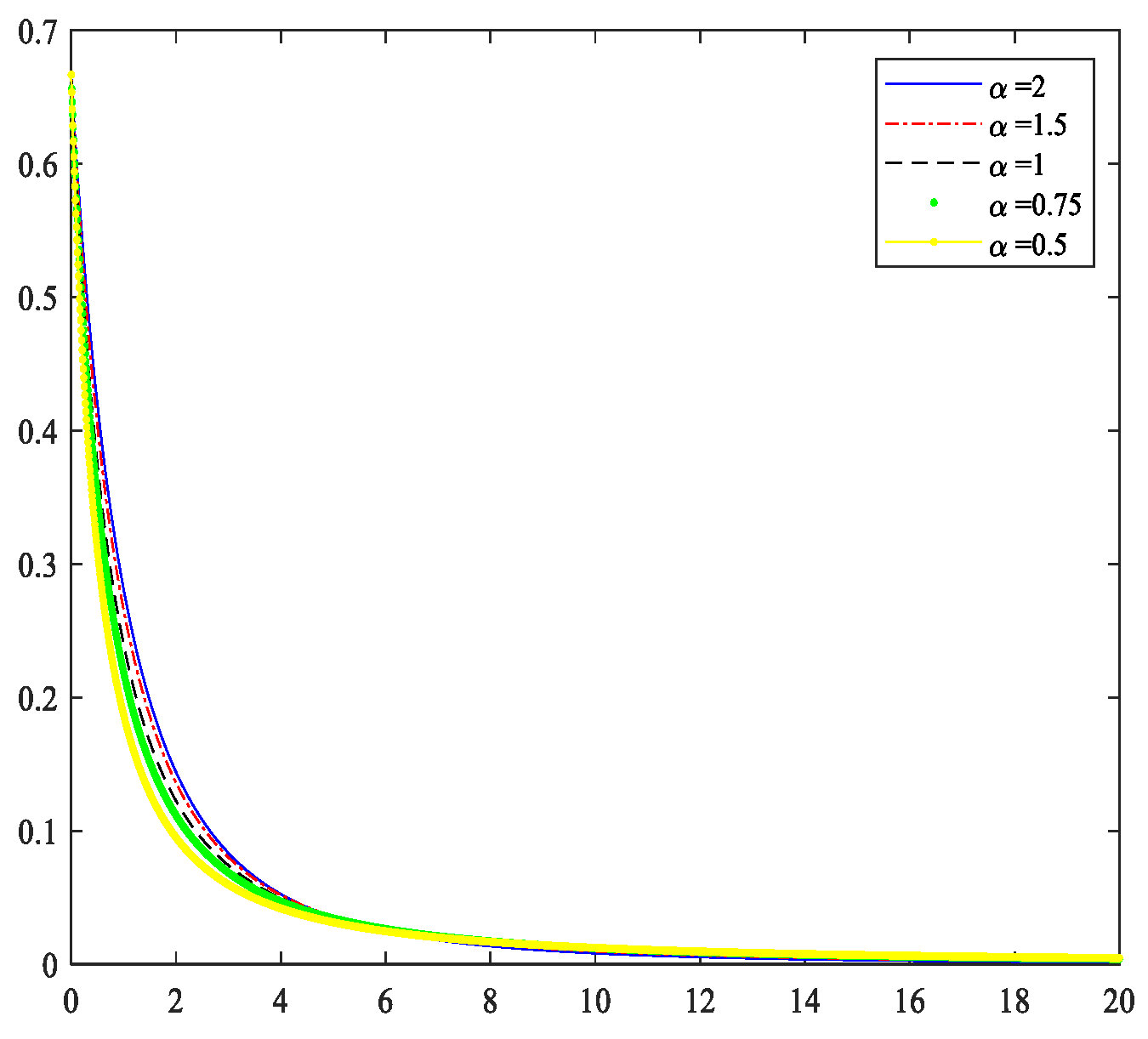
2.3. Incremental Distribution of the Generalized Pareto

The subsequent iterative prediction model is expressed by the incremental form. So, in this section, we use statistical methods to obtain the incremental distribution of GPD. The main steps can be summarized as follows:
(1).
Generate GPD-compliant time series.
(2).
Determine the time interval τ , and the two-state quantities separated by τ in the sequence are differentiated multiple times, i.e., Δ x ( t ) = x ( t + τ ) x ( t ) . Repeat the above process to make multiple differences of the generated time series to form an incremental set.
(3).
Draw the histogram of the incremental set, in order to obtain the probability density map of the set and select a known distribution to fit it according to the characteristics of the probability distribution.
(4).
After proposing a distribution that meets the characteristics of the incremental data, the χ 2 test method [38,39] is used to test the distribution fit.
In the following, we use the GPD with parameters α = 1.5 ,   δ = 2 ,   μ = 10 . The corresponding time series is shown in Figure 3.
The GPD is given in Figure 3 and the GPD incremental data are plotted in Figure 4. The peak and high variability of the GPD time series data indicate that the distribution is heavy-tailed. At the same time, the GPD time series are not similar to white (pure random) noise, and the obvious clustering in the data indicates the self-similarity of the GPD time series.
It can be seen from Figure 5 that the probability density of the GPD increment has the characteristics of symmetry and tail weight, and in order not to affect the meaning of the parameters in the probability density, we can choose those with these two characteristics and a similar probability density function. Generalized double Pareto distribution is used, then to fit the date. The PDF is as follows [34]:
f G D P ( x | δ , α , μ ) = 1 2 δ [ 1 + | x μ | α δ ] 1 α
where δ > 0 is a scale parameter, α > 0 is a tail parameter, and the location μ represents the mean value of the random variable. Similarly, when x , f ( x ) follows Equation (3). The influence of δ and α on the distribution is consistent with GPD (Figure 6 and Figure 7).
It can be seen from Figure 5 that the position parameter is μ = 0 in the generalized double Pareto distribution. And because when x = 0 ,   f ( x ) = 1 / 2 δ , the probability value of 0 can be used to estimate δ . It can be seen from Figure 4, their peak value of the GPD increment sequence is due to the corresponding peak value of the GPD time sequence and their tails are similar in distribution, so their corresponding tail parameters α are the same. It can be concluded that the values of the parameters in the generalized double Pareto distribution are μ = 0 ,   δ = 1.1638 and α = 1.5 . To form the χ 2 test [38,39] between the empirical distribution in Figure 5 and the generalized double Pareto distribution with known parameters, the process is as follows:
(1).
Make the following test assumptions, H0: Figure 4 obeys the generalized double Pareto distribution, H1: Figure 4 does not obey the generalized double Pareto distribution.
(2).
Partition the value range of the overall data X in Figure 4 into   k intervals [ a i 1 , a i ], i = 1 , 2 , k ( a i 1 , a i can be , + ), where the size of k is not strictly specified, but if it is too small, it will make the test too rough, and if it is too large, it will increase random errors. Usually, the sample size n is larger, and k can be slightly larger, but generally 5 k 16 . In this example, there are four grouping cases k = 10, 12, 14, 16.
(3).
Assuming that H 0 holds, calculate the theoretical probability p i and theoretical frequency n p i of each interval:
p i = x = a i 1 a i f G D P ( x | δ , α , μ )
(4).
According to the sample observation values ( x 1 ,   x 2 , ,   x n ) in Figure 4, calculate the actual frequency v i of falling in the interval [ a i 1 , a i ], and then calculate the observation value of the statistic χ 2 :
χ 2 = i = 1 k ( n p i v i ) 2 n p i
(5).
Accordingly, choosing 95% based on confidence, check the χ 2 distribution Table, and get   χ 2 ( k r 1 ) , where r is the number of unknown parameters in the generalized Pareto distribution PDF, because the generalized Pareto distribution PDF parameters are known, so   r = 0 . The four sets of   χ 2 ( k 1 ) values found out from the table and the χ 2 values obtained from the four experiments are compared in Table 1:
It can be seen from Table 1 that the experimental results show that the χ 2 value is always smaller than the χ 2 ( k 1 ) value obtained from the look-up Table, so there is a 95% probability that H0 holds. In a statistical sense, it can be said that the time series of Figure 4 obeys the generalized double Pareto distribution.

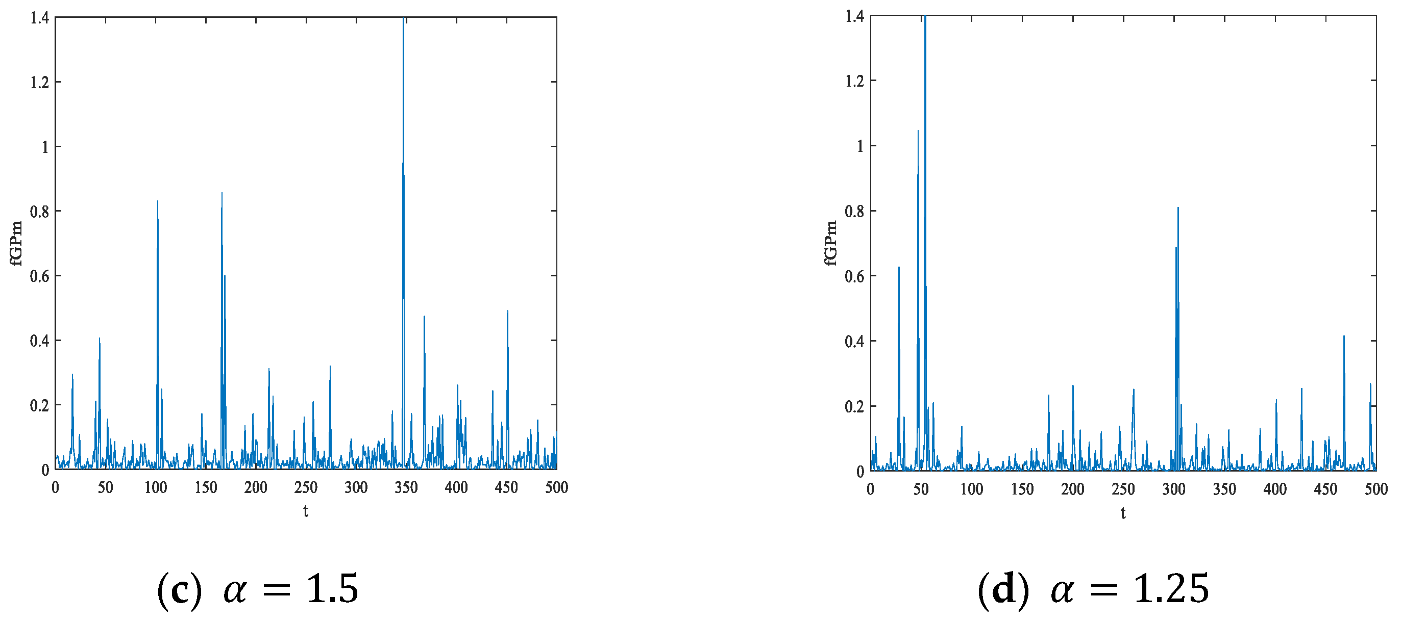
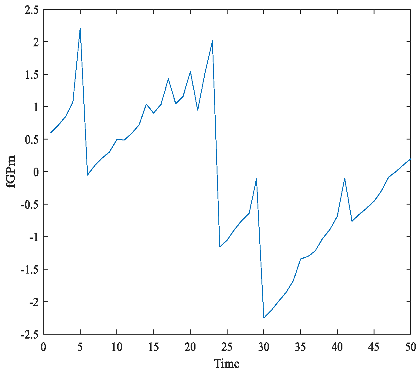
3. Fractional Generalized Pareto Motion

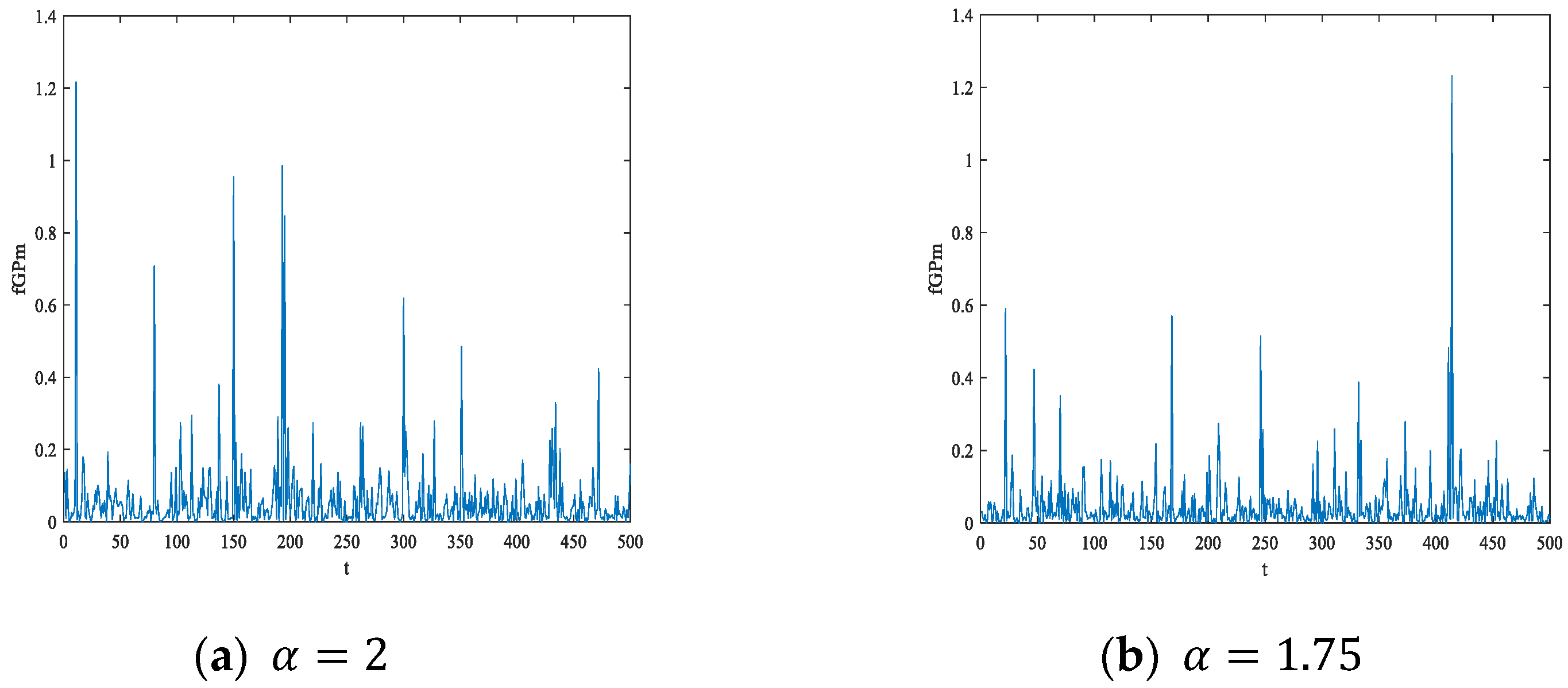
3.1. Fractional Generalized Pareto Motion Model

We define a parametric family of fractional Brownian motion in terms of the stochastic Weyl integral [7,40].
B H ( t ) = { a [ ( t s ) + H 1 2 ( s ) + H 1 2 ] + b [ ( t s ) H 1 2 ( s ) H 1 2 ] } B ( d s )
where a and b are arbitrary constants, x + H 1 / 2 = 0   for   x 0   and   x + H 1 2 = x H 1 2   for   x > 0 , B ( d s ) is Gaussian with mean 0 and variance | d s | , H is the self-similarity parameter. The integral expression analogous to fractional Brownian motion is generalized to the method of fractional Levy stable motion [8,21,22], and similarly, the integral expression of fGPm can also be obtained. In addition, the relationship between H and α in the generalized Pareto motion is H = 1 α . The representation of fGPm is acquired by transforming the exponent in the Equation (5) from H 1 / 2 to H 1 / α , and a GPD random measure with the location parameter μ = 0 replaces the standard Brownian random measure as the driving function. The fGPm is defined by:
P H , α ( t ) = { a [ ( t s ) + H 1 α ( s ) + H 1 α ] + b [ ( t s ) H 1 α ( s ) H 1 α ] } p ( d s )
where p ( d s ) is a GPD random process with the location parameter μ = 0 and scale parameter = | d s | . When t > s > 0 , we discretize s as { 0 , 1 , 2 ,   ,   t } , and Equation (11) can be written as:
P H , α ( t ) = s = 0 t a ( t s ) H 1 α b ( s ) H 1 α p ( 1 )
where a ( t s ) H 1 α b ( s ) H 1 α can also be written as a constant sequence A n = { a 0 , a 1 , , a t } , to obtain:
P H , α ( t ) = ( a 0 + a 1 p + + a n ) p ( 1 ) = A n p ( 1 )
Therefore, fGPm in Equation (11) can be regarded as a superposition of GPD with different weighting coefficients, where μ and δ of fGPm are 0 and d s , respectively. It can be concluded that the fGPm has infinite variance and its probability distribution is subject to GPD. Similarly, we can also define the fGPm as the following Riemann-Liouville fractional integral [41]:
P H , α ( t ) = 1 Γ ( H + 1 2 ) 0 t ( t τ ) H 1 2 p ( d τ )
where p ( d τ ) is the GPD motion with the location parameter μ = 0 and the scale parameter = d τ . Γ ( · ) is the gamma function, the gamma function is defined as Γ ( x ) = 0 + t x 1 e t d t ( x > 0 ) . Figure 8 shows the fGPm sequence generated with different α values for H = 0.75 . We should notice that the random walk of the fGPm sequence increases as α increases.

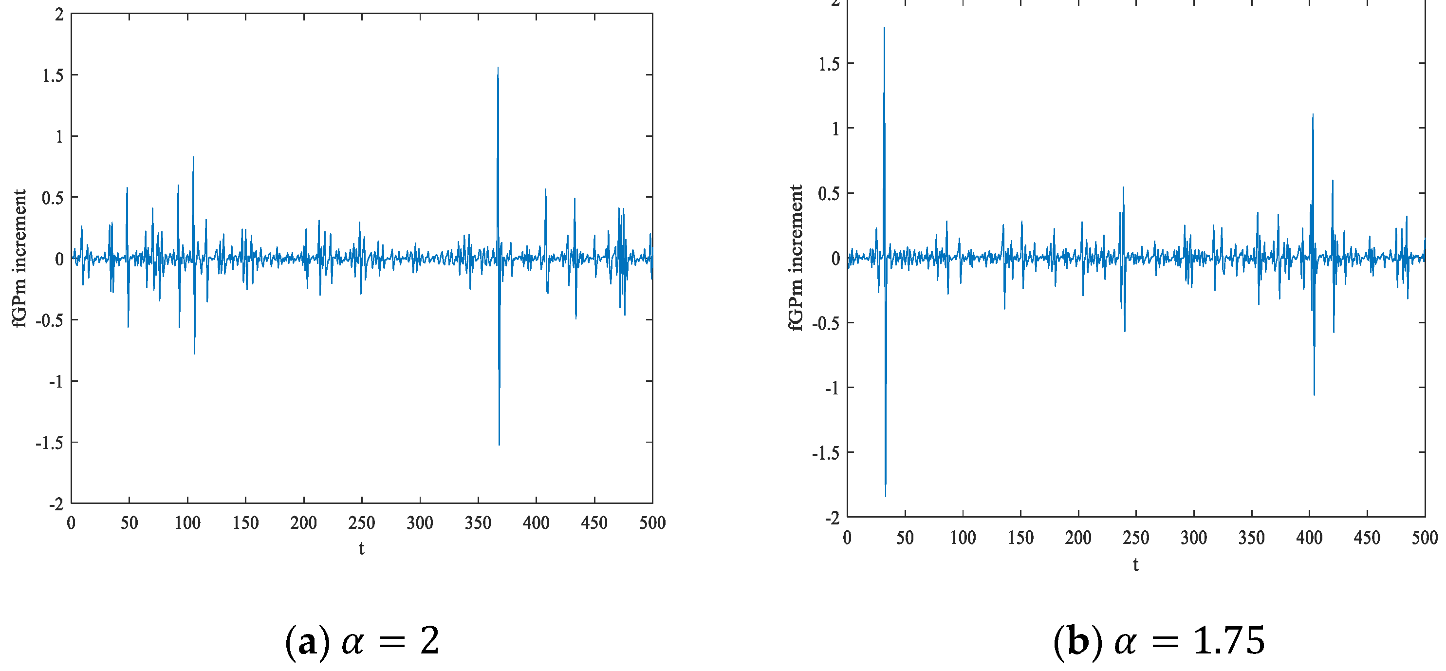
3.2. Fractional Generalized Pareto Motion Incremental Processes Model

The 1-step incremental model of fGPm is obtained from the identity X H , α ( t ) = P H , α ( t + 1 ) P H , α ( t ) :
X H , α ( t ) = P H , α ( t + 1 ) P H , α ( t ) = { a [ ( t + 1 s ) + H 1 / α ( s ) + H 1 / α ] + b [ ( t + 1 s ) H 1 / α ( s ) H 1 / α ] } ω α ( s ) d s
where ω α ( s ) = p [ d ( s + 1 ) ] p ( d s ) ] . From Section 2.1, we can see that ω α ( s ) follows the generalized double Pareto distribution with position parameter μ = 0 and scale parameter δ = 1 . Figure 9 shows the fGPm incremental sequence generated with different α , where H = 0.75 . We observe that the influence of noise increases as the parameters increases.

3.3. Long-Range Dependence and Self-Similarity of Fractional Generalized Pareto Motion

The basic idea of self-similarity for stochastic processes can be seen as the invariance in distribution under suitable scaling of time. Self-similarity can be expressed as:
x ( t ) a H x ( a t )
where H (Hurst exponent) is the self-similarity parameter, denotes equality in distribution. Several methods can be used to calculate the self-similarly parameter H such as the absolute value method, the periodogram estimation method, the wavelet estimation method, rescaled range method etc. [42,43,44]. Since the best accuracy is achieved by the rescaled range method [36], we use this method for the estimation of the self-similar parameters in LRD random processes.
Generalized Pareto motion is a self-similar process with a self-similarity parameter 1 α , namely, p ( t ) a 1 / α p ( a t ) for all a > 0 . As can be seen from Figure 8, the fGPm does not resemble white (pure random) noise as the clustering in data is clearly visible, this indicates the existence of self-similarity. Following N. Laskin et al.’s proof that fractional Levy stable motion is a self-similar process [41], fGPm self-similarity parameters are obtained as follows:
P H , α ( c t ) = 1 Γ ( H + 1 2 ) 0 c t d p ( τ ) ( c t τ ) H 1 2 = c H 1 2 + 1 a Γ ( H + 1 2 ) 0 t d p ( τ ) ( t τ ) H 1 2 = c H 1 2 + 1 a P H , α ( t )
Equation (17) shows that the fGPm is a self-similar process with self-similarly parameter H 1 / 2 + 1 / α . Similarly, the fGPm incremental process is also self-similar with parameter H 1 / 2 + 1 / α .
As shown in Equation (6), the LRD of fGPm is closely related to its integral kernel a [ ( t s ) + H 1 α ( s ) + H 1 α ] + b [ ( t s ) H 1 α ( s ) H 1 α ] . When t > s , if H   1 α , fGPm always shows that the value of the current time t is always related to the value of all the times s in the past, so that the integral kernel has a strong memory. We say that fGPm has LRD when H > 1 α and negative dependence when H < 1 α . Moreover, the sequence of the self-similar parameter H     ( 1 / 2 ,   1 ) has LRD characteristics [17,18]. Therefore, we restrict H to the interval ( 1 / 2 ,   1 ) with H > 1 α so that α belongs to ( 1 , 2 ) . The key feature of the fGPm model is that parameters α ,   H are not independent since the fGPm has the LRD condition for α H > 1 .

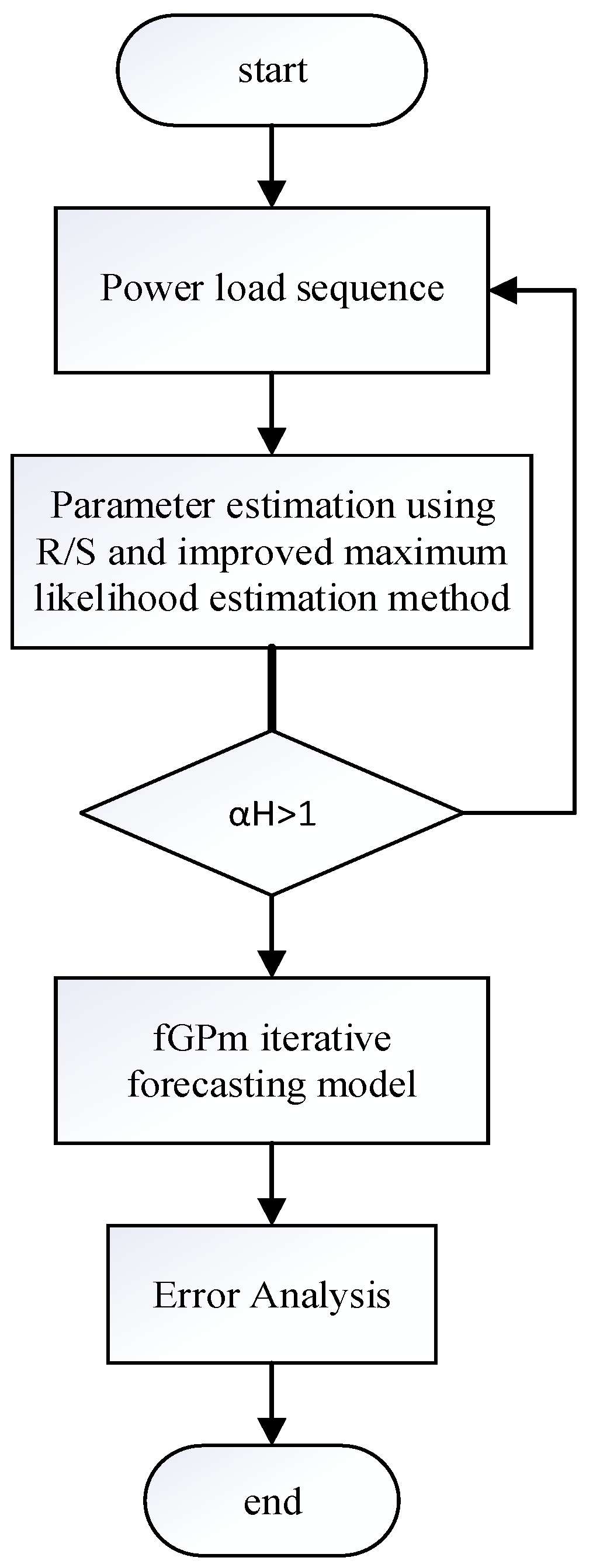
4. Iterative Forecasting Model based on Fractional Generalized Pareto Motion

4.1. Iterative Forecasting Model

A. A. Stanislavsky et al. [12] proposed the FARIMA model with Pareto noise, which is a discrete-time analog of the fractional Langevin equation, in which the non-Gaussian statistics and the LRD are considered [25]. Therefore, let us consider the following Langevin-type stochastic differential equation [26,27] driven by GPD motion:
d X ( t ) = b ( t , X ( t ) ) d t + δ ( t , X ( t ) ) d p α ( t )   ,   X ( 0 ) = X 0
where d p α ( t ) stands for the increments of generalized Pareto motion p α ( t ) . By replacing P H , α ( t ) to p α ( t ) , we obtain the Langevin-type stochastic differential equation driven by fGPm:
d X H , α ( t ) = b ( t , X H , α ( t ) ) d t + δ ( t , X H , α ( t ) ) d P H , α ( t )   ,   X H , α ( 0 ) = X 0
where b ( t , X ( t ) ) and δ ( t , X ( t ) ) represent the drift and diffusion functions, respectively. The Black-Scholes model [28,29] was generalized to the fractional Black-Scholes model by Dai et al. [45,46,47], based on the stochastic equation:
d S t = μ S t d t + δ S t d B H ( t )
where μ indicates the expected return rate, δ is the volatility rate. In fGPm, the iterative prediction model is based on incremental modeling, so the parameters of the differential equation correspond to the parameters of the fGPm increment. In Section 2.3, we use the generalized double Pareto distribution to fit the increment of GPD. Figure 9 shows that the increment of fGPm also obeys the generalized double Pareto distribution. In addition, when the range of the generalized double Pareto α is ( 0 ,   2 ) , it is asymptotically in the attractive domain of Levy’s stable distribution [7,12]. Therefore, μ represents the mean value of random variables, the parameter δ represent the diffusion coefficient. Consequently, Equation (20) can be rewritten as follows:
d X H , α ( t ) = μ X H , α ( t ) d t + δ X H , α ( t ) d P H , α ( t )
where μ , δ are constants. By using the Maruyama symbol [33] d B t = w ( t ) ( d t ) 1 / 2 ( ω ( t ) represents Gaussian white noise), we get:
0 t f ( τ ) ( d τ ) a = a 0 τ ( t τ ) a 1 f ( τ ) d τ
and
d x = f ( t ) ( d t ) a
where 0 < a < 1 represents the self-similar parameter of x . f ( t ) denote a continuous function. The incremental expression of fGPm can be obtained by replacing f ( t ) with w α ( t ) :
d P H , α = w α ( t ) ( d t ) H 1 2 + 1 α
It can be seen from Figure 9 that the increment of fGPm obeys the generalized double Pareto distribution, so ω α ( s ) follows the generalized double Pareto distribution with position parameter μ = 0 and scale parameter δ = 1 .
Equation (18) can be discretized as:
Δ X H , α ( t ) = μ X H , α ( t ) Δ t + δ X H , α ( t ) w α ( t ) ( Δ t ) H 1 2 1 α
The iterative predictive model was obtained from the identity Δ X ( t ) = X ( t + 1 ) X ( t ) :
P H , α ( t + 1 ) = P H , α ( t ) + μ P H , α ( t ) Δ t + δ P H , α ( t ) w α ( t ) ( Δ t ) H 1 2 + 1 α
By using Monte Carlo simulation [48], most likely curves for multiple time series can be generated. Assuming that α = 1.5 , µ = 0.4586 , δ = 0.0396 , H = 0.75 , X 0 = 0.6 , we performed 50 simulations by the Monte Carlo method and obtained the results in Figure 10. We can see that the data simulated by the fGPm iterative prediction model has high jumps, and the model will have good predictability for high jump data.

4.2. Parameter Estimation of μ,δ,α
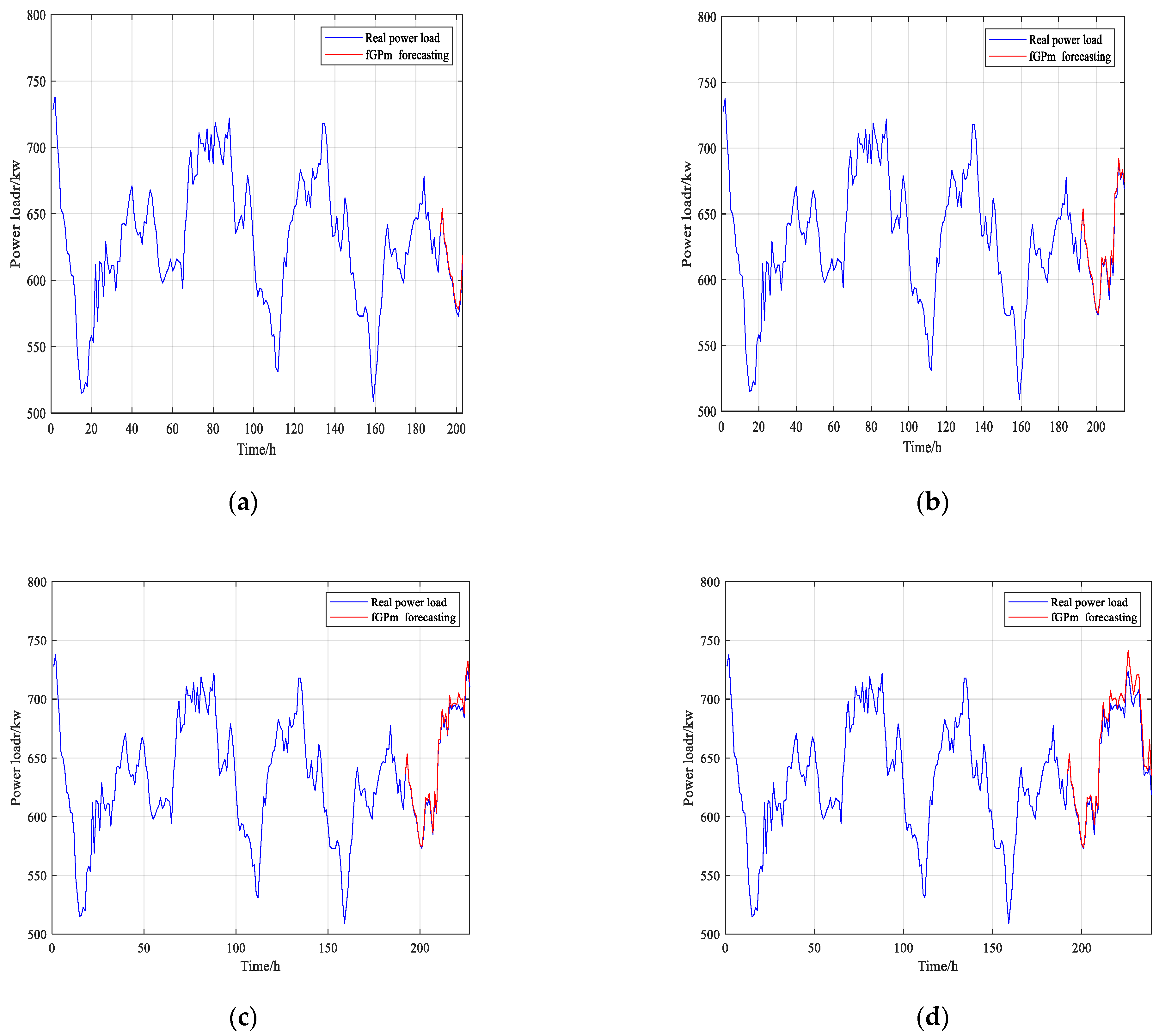
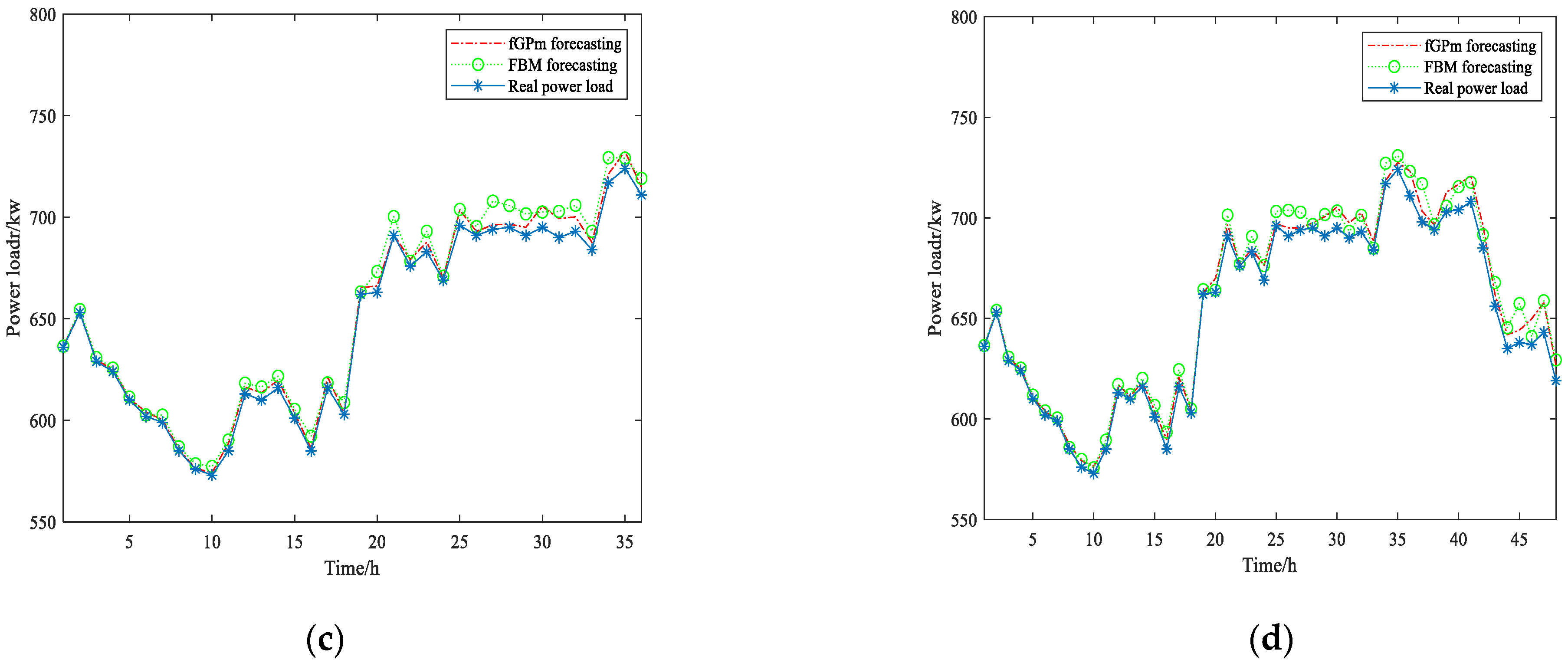
As mentioned in 3.1., μ is the mean of the series, so its estimated value can be expressed as the mean of the time series. In addition, the estimation of α and δ can be done by the most common maximum likelihood estimation method [30,31]. But there may be no maximum likelihood estimates for α and δ . To find a solution, Davison [32] pointed out that by a change of parameters to θ = 1 / α δ and α = α , the problem is reduced to a unidimensional search. We search for θ , which gives a local maximum of the profile log-likelihood (the log-likelihood maximized over 1 / α ). The specific process is:
Step 1: Let x i | i = 1 N be the sampling data for the fGPm,
Step 2: let x ( 1 )   x ( 2 )   · · · x ( N ) be the order statistics.
Step 3: μ estimation:
μ = 1 N i = 1 N x i
Step 4: α and δ estimation:
L * ( θ ) = l o g 2 N i = 1 N log ( 1 θ x i ) N l o g [ 1 N θ i = 1 N log ( 1 θ x i ) ]
For θ < 1 / x ( N ) . By assuming that a local maximum θ ^ of (27) can be found, then it follows that
α ^ = N i = 1 N log ( 1 θ ^ x i )
δ ^ = 2 α ^ θ ^

5. Case Study

To verify the validity of the fGPm forecasting model, in this section we give the results of an experiment considering power load curves and predictions in the future of 6, 12, 18 and 24 h model for the two cased. The actual power load data is collected by the Eastern Slovak Electric Power Company [35] and is sampled every 30 min. By selecting the historical power load data in two cases (weekdays-case1 and weekends-case2), the parameters of the are estimated using R/S and the improved maximum likelihood estimation method. The calculated parameters are shown in Table 2. According to the condition α H > 1 , both sets of data have LRD characteristics. Therefore, the two sets of data are modeled by the fGPm forecast model. The experimental process is shown in Figure 11.

5.1. Case 1: Weekdays

The power load of the first week of working days in January is used as the input sequence: that is, the power load from Monday to Thursday is used as historical data to predict the power load on Friday. Since the power consumption on weekdays is similar, and Monday to Thursday are close to Friday, it can accurately reflect the trend of power load data. Replacing this set with an iterative predictive model, we predict the trend of data sets for the next 6, 12, 18 and 24 h. The 24-h forecast trend of historical data is shown in Figure 12. At the same time, the fractional Brownian iterative prediction model [23,36] is used to repeat the above process and the results are compared with the fGPm prediction results in Figure 13. The maximum and average absolute percentage errors of the prediction results are shown in Table 3. The results show that the fGPm iterative prediction model has a good effect on the high-jump power load data prediction.

5.2. Case 2: Weekends

We repeated the analysis of Case 1, using the weekends of the first two weeks of January to predict the power load trend in the next weekend. Since the electric load trends on weekends are similar, the electric load sequence between each weekend also has LRD characteristics. Therefore, it can also be used to predict power load trends. The results of weekend power load forecasting are shown in Figure 14. The comparison of the two forecasting models is shown in Figure 15. The error analysis results are reported in Table 4.

6. Conclusions

The main contributions of this paper are as follows. Firstly, the incremental distribution of GPD is obtained using statistical methods and the LRD characteristics of the generalized Pareto motion are analyzed according to the heavy-tailed characteristics of its distribution: the mathematical relationship H = 1 α of the self-similarly parameter H and the tail parameter α is obtained. Secondly, analogously to the method of generalizing fBm’s integral expression to fractional Levy stable motion, the integral expression of fGPm is obtained, discretized and analyzed, revealing that fGPm has infinite variance. Third, the fGPm-driven Langevin-type SDE has been used to establish the fGPm iterative prediction model and the parameter estimation method in the Langevin-type SDE was also provided. The prediction model for considered only the case of α ( 1 , 2 ) : the case of α ( 0 , 1 ) has yet to be studied in the future.
In order to verify the effectiveness of the fGPm prediction model, two different scenarios (weekdays and weekends) of power load data were considered in the case study. The prediction accuracy in the study is good, indicating that the model is universally applicable. At the same time, the comparison of the fGPm iterative prediction model with the fractional Brownian iterative prediction model highlights the superiority of the prediction model in this paper for high-jump data prediction. Wind speed prediction is a challenging job at present. Due to the strong randomness and intermittency of wind speed, the wind speed sequence is high-jump data. This model may have a good prediction effect on this kind of problem.

Author Contributions

W.S.: Conceptualization, Data curation, Investigation; S.D.: Writing—original draft, Formal analysis, Software; D.C.: Project administration, Resources, Supervision; E.Z.: Writing—review & editing, Formal analysis; W.Y.: Funding acquisition, Supervision, Software; F.C.: Software, Writing—original draft. All authors have read and agreed to the published version of the manuscript.

Funding

This research was funded by Natural Science Foundation of Fujian Province, grant number 2021J01530, and the Science and Technology Project of Quanzhou City under Grant 2020C011R and 2019CT003.

Data Availability Statement

Available online: http://neuron-ai.tuke.sk/competition (accessed on 8 July 2022).

Acknowledgments

First of all, thanks to the Eastern Slovak Electric Power Company for the data provided. Available online: http://neuron-ai.tuke.sk/competition (7/8/1997).

Conflicts of Interest

The authors declare no conflict of interest.

References

  1. Morf, H. Sunshine and cloud cover prediction based on Markov processes. Sol. Energy 2014, 110, 615–626. [Google Scholar] [CrossRef]
  2. Tsai, C.-C.; Tseng, S.-T.; Balakrishnan, N. Optimal Design for Degradation Tests Based on Gamma Processes with Random Effects. IEEE Trans. Reliab. 2012, 61, 604–613. [Google Scholar] [CrossRef]
  3. Ye, Z.-S.; Wang, Y.; Tsui, K.-L.; Pecht, M. Degradation Data Analysis Using Wiener Processes With Measurement Errors. IEEE Trans. Reliab. 2013, 62, 772–780. [Google Scholar] [CrossRef]
  4. Sottinen, T.; Viitasaari, L. Prediction law of fractional Brownian motion. Stat. Probab. Lett. 2017, 129, 155–166. [Google Scholar] [CrossRef]
  5. Lahiri, S.N.; Das, U.; Nordman, D.J. Empirical Likelihood for a Long Range Dependent Process Subordinated to a Gaussian Process. J. Time Ser. Anal. 2019, 40, 447–466. [Google Scholar] [CrossRef]
  6. Li, M. Record length requirement of long-range dependent teletraffic. Phys. A Stat. Mech. Its Appl. 2017, 472, 164–187. [Google Scholar] [CrossRef]
  7. Samorodnitsky, G.; Taqqu, M.S. Linear Models with Long-Range Dependence and with Finite or Infinite Variance. In New Directions in Time Series Analysis; Springer: New York, NY, USA, 1993; Volume 46, pp. 325–340. [Google Scholar] [CrossRef]
  8. Samorodnitsky, G.; Taqqu, M.S. Stable Non-Gaussian Random Processes: Stochastic Models with Infinite Variance; Routledge: London, UK, 2017. [Google Scholar] [CrossRef]
  9. Embrechts, P.; Klüppelberg, C.; Mikosch, T. Modelling Extremal Events for Insurance and Finance; Springer Science & Business Media: Berlin/Heidelberg, Germany, 2003. [Google Scholar] [CrossRef]
  10. Kotz, S.; Nadarajah, S. Extreme Value Distributions: Theory and Applications; World Scientific Publishing Company: Singapore, 2000. [Google Scholar] [CrossRef] [Green Version]
  11. Ji, J.; Wang, D.; Xu, D.; Xu, C. Combining a self-exciting point process with the truncated generalized Pareto distribution: An extreme risk analysis under price limits. J. Empir. Financ. 2020, 57, 52–70. [Google Scholar] [CrossRef]
  12. Stanislavsky, A.A.; Burnecki, K.; Magdziarz, M.; Weron, A.; Weron, K. Statistical Modeling of Solar Flare Activity from Empirical Time Series of Soft X-ray Solar Emission. Astrophys. J. Lett. 2009, 693, 1877–1882. [Google Scholar] [CrossRef]
  13. Beran, J. Statistical Methods for Data with Long-Range Dependence. Stat. Sci. 1992, 7, 404–416. [Google Scholar] [CrossRef]
  14. Liu, H.; Song, W.; Zio, E. Generalized Cauchy difference iterative forecasting model for wind speed based on fractal time series. Nonlinear Dyn. 2021, 103, 759–773. [Google Scholar] [CrossRef]
  15. Samorodnitsky, G.; Taqqu, M.S. Stable Non-Gaussian Random Processes; Chapman & Hall: New York, NY, USA, 1994. [Google Scholar] [CrossRef]
  16. Loiseau, P.; Gonçalves, P.; Dewaele, G.; Borgnat, P.; Abry, P.; Primet, P.V.B. Investigating self-similarity and heavy-tailed dis-tributions on a large-scale experimental facility. IEEE/ACM Trans. Netw. 2010, 18, 1261–1274. [Google Scholar] [CrossRef]
  17. Karasaridis, A.; Hatzinakos, D. Network heavy traffic modeling using α-stable self-similar processes. IEEE Trans. Commun. 2001, 49, 1203–1214. [Google Scholar] [CrossRef]
  18. Liu, H.; Song, W.Q.; Zio, E. Fractional Lévy stable motion with LRD for RUL and reliability analysis of li-ion battery. ISA Tran. 2022, 125, 360–370. [Google Scholar] [CrossRef] [PubMed]
  19. Adler, R.; Feldman, R.; Taqqu, M.S. On Estimating the Intensity of Long-Range Dependence in Finite and Infinite Variance Time Series. In A Practical Guide to Heavy Tails: Statistical Techniques and Applications; Springer Science & Business Media: Berlin/Heidelberg, Germany, 1998. [Google Scholar]
  20. Janicki, A.; Weron, A. Can One See alpha-stable Variables and Processes? Stat. Sci. 1994, 9, 109–126. [Google Scholar] [CrossRef]
  21. Benassi, A.; Cohen, S.; Istas, J. On roughness indexes for fractional fields. Bernoalli 2004, 10, 357–373. [Google Scholar]
  22. Kogon, S.; Manolakis, D. Signal modeling with self-similar α-stable processes: The fractional Levy stable motion model. IEEE Trans. Signal Process. 1996, 44, 1006–1010. [Google Scholar] [CrossRef]
  23. Liu, H.; Song, W.; Zhang, Y.; Kudreyko, A. Generalized Cauchy Degradation Model With Long-Range Dependence and Maximum Lyapunov Exponent for Remaining Useful Life. IEEE Trans. Instrum. Meas. 2021, 70, 9369345. [Google Scholar] [CrossRef]
  24. Duan, S.; Song, W.; Zio, E.; Cattani, C.; Li, M. Product technical life prediction based on multi-modes and fractional Lévy stable motion. Mech. Syst. Signal Process. 2021, 161, 107974. [Google Scholar] [CrossRef]
  25. Magdziarz, M.; Weron, A. Fractional Langevin equation with α-stable noise. A link to fractional ARIMA time series. Stud. Math. 2007, 181, 47–60. [Google Scholar] [CrossRef]
  26. Weron, A.; Burnecki, K.; Mercik, S.; Weron, K. Complete description of all self-similar models driven by Lévy stable noise. Phys. Rev. E 2005, 71, 016113. [Google Scholar] [CrossRef] [PubMed]
  27. Lee, P.M.; Janicki, A.; Weron, A. Simulation and Chaotic Behaviour of α-Stable Stochastic Processes; HSC Books: Wroclaw, Poland, 1994. [Google Scholar] [CrossRef]
  28. Black, F.; Scholes, M. The Pricing of Options and Corporate Liabilities. J. Political Econ. 2012, 81, 637–654. [Google Scholar] [CrossRef]
  29. Jumarie, G. Merton’s model of optimal portfolio in a Black-Scholes Market driven by a fractional Brownian motion with short-range dependence. Insur. Math. Econ. 2005, 37, 585–598. [Google Scholar] [CrossRef]
  30. Grimshaw, S.D. Computing Maximum Likelihood Estimates for the Generalized Pareto Distribution. Technometrics 1993, 35, 185–191. [Google Scholar] [CrossRef]
  31. Moharram, S.; Gosain, A.; Kapoor, P. A comparative study for the estimators of the Generalized Pareto distribution. J. Hydrol. 1993, 150, 169–185. [Google Scholar] [CrossRef]
  32. Davison, A.C. Modelling Excesses over High Thresholds, with an Application. In Statistical Extremes and Applications; Springer: Dordrecht, The Netherlands, 1984; pp. 461–482. [Google Scholar] [CrossRef]
  33. Jumarie, G. On the representation of fractional Brownian motion as an integral with respect to (dt)a. Stat. Extrem. Appl. 2005, 18, 739–748. [Google Scholar] [CrossRef]
  34. Armagan, A.; Dunson, D.B.; Lee, J. Generalized double Pareto shrinkage. Stat. Sin. 2013, 23, 119–143. [Google Scholar] [CrossRef]
  35. Lotfi, A. Application of Learning Fuzzy Inference Systems in Electricity Load Forecast; Nottingham Trent University: Nottingham, UK, 2001. [Google Scholar]
  36. Song, W.; Liu, H.; Zio, E. Long-range dependence and heavy tail characteristics for remaining useful life prediction in rolling bearing degradation. Appl. Math. Model. 2022, 102, 268–284. [Google Scholar] [CrossRef]
  37. Korn, G.A.; Korn, T.M. Mathematical Handbook for Scientists and Engineers; McGraw-Hill: New York, NY, USA, 1961. [Google Scholar] [CrossRef]
  38. Best, D.; Rayner, J. Are Two Classes Enough for the X2Goodness of Fit Test? Stat. Neerlandica 1981, 35, 157–163. [Google Scholar] [CrossRef]
  39. Hsuan, A.; Robson, D.S. The X2-goodness-of-fit tests with moment type estimators. Commun. Stat. Theory Methods 2007. [Google Scholar] [CrossRef]
  40. Marquardt, T. Fractional Lévy processes with an application to long memory moving average processes. Bernoulli 2006, 12, 1099–1126. [Google Scholar] [CrossRef]
  41. Laskin, N.; Lambadaris, I.; Harmantzis, F.; Devetsikiotis, M. Fractional Lévy motion and its application to network traffic modeling. Comput. Newt. 2002, 40, 363–375. [Google Scholar] [CrossRef]
  42. Li, M.; Zhang, P.; Leng, J. Improving autocorrelation regression for the Hurst parameter estimation of long-range dependent time series based on golden section search. Phys. A Stat. Mech. Its Appl. 2016, 445, 189–199. [Google Scholar] [CrossRef]
  43. Mandelbrot, B.B.; Wallis, J.R. Robustness of the rescaled range R/S in the measurement of noncyclic long run statistical dependence. Water Resour. Res. 1969, 5, 967–988. [Google Scholar] [CrossRef]
  44. Stoev, S.; Taqqu, M.S.; Park, C.; Marron, J. On the wavelet spectrum diagnostic for Hurst parameter estimation in the analysis of Internet traffic. Comput. Netw. 2005, 48, 423–445. [Google Scholar] [CrossRef]
  45. Dai, W.; Heyde, C.C. Itô’s formula with respect to fractional Brownian motion and its application. J. Appl. Math. Stoch. Anal. 1996, 9, 439–448. [Google Scholar] [CrossRef]
  46. Wang, X.-T.; Qiu, W.-Y.; Ren, F.-Y. Option pricing of fractional version of the Black–Scholes model with Hurst exponent H being in (13,12). Chaos Solitons Fractals 2001, 12, 599–608. [Google Scholar] [CrossRef]
  47. Yan, L.; Shen, G.; He, K. Itô’s formula for a sub-fractional Brownian motion. Commun. Stoch. Anal. 2011, 5, 135–159. [Google Scholar] [CrossRef]
  48. Lemieux, C. Monte Carlo and Quasi-Monte Carlo Sampling; Springer: New York, NY, USA, 2009. [Google Scholar] [CrossRef] [Green Version]
Figure 1. Comparison of δ value in GPD PDF plots.
Fractalfract 06 00471 g001
Figure 2. Comparison of α value in GPD PDF plots.
Fractalfract 06 00471 g002
Figure 3. GP time series.
Fractalfract 06 00471 g003
Figure 4. GP increment time series.
Fractalfract 06 00471 g004
Figure 5. Probability density of GP increment.
Fractalfract 06 00471 g005
Figure 6. Comparison of δ value in GPD PDF plots.
Fractalfract 06 00471 g006
Figure 7. Comparison of α value in GPD PDF plots.
Fractalfract 06 00471 g007
Figure 8. fGPm generated with different α = 2 ,   1.75   ,   1.5   ,   1.25 , respectively, H = 0.75 .
Fractalfract 06 00471 g008aFractalfract 06 00471 g008b
Figure 9. fGPm increment data generated with different α = 2 ,   1.75   ,   1.5   ,   1.25 , respectively, H = 0.75 .
Fractalfract 06 00471 g009aFractalfract 06 00471 g009b
Figure 10. fGPm sequences generated with α = 1.5   ,   µ = 0.4586 ,   δ = 0.0396   ,   H = 0.75   ,   X 0 = 0.6 , by the Monte Carlo simulation method.
Fractalfract 06 00471 g010
Figure 11. Forecasting process.
Fractalfract 06 00471 g011
Figure 12. The 96-h power load of the actual working day of the fGPm forecast model and the subsequent forecast 24-h trend chart. (a) 6 h (b) 12 h (c) 18 h (d) 24 h.
Fractalfract 06 00471 g012
Figure 13. Comparison of two forecasting models in working days. (a) 6 h (b) 12 h (c) 18 h (d) 24 h.
Fractalfract 06 00471 g013aFractalfract 06 00471 g013b
Figure 14. Actual weekend 96 h power load and subsequent forecast 24 h trend chart. (a) 6 h (b) 12 h (c) 18 h (d) 24 h.
Fractalfract 06 00471 g014aFractalfract 06 00471 g014b
Figure 15. Comparison of two forecasting models in weekend. (a) 6 h (b) 12 h (c) 18 h (d) 24 h.
Fractalfract 06 00471 g015
Table 1. Look-up Table χ2 (k−1) value and experimental χ2 value comparison.
Experimental k Valuek = 10k = 12k = 14k = 16
χ 2 ( k 1 ) 16.9219.6822.3625
χ 2 15.4215.8316.1518.21
Table 2. Parameter estimation of forecasting model.
H α μ δ
Case 10.82421.7322639.68253.0220
Case 20.78831.7178751.54192.8802
Table 3. The workday forecasting relative error (%) of power loads on adjacent dates.
Forecast TimeNamefGPm ForecastingFBM Forecasting
6 hMax error percentage0.931.26
6 hMean error percentage0.420.44
12 hMax error percentage1.401.95
12 hMean error percentage0.460.60
18 hMax error percentage1.482.00
18 hMean error percentage0.470.89
24 hMax error percentage2.283.04
24 hMean error percentage0.740.95
Table 4. The weekend forecasting relative error (%) of power loads on adjacent dates.
Forecast TimeNamefGPm ForecastingFBM Forecasting
6 hMax error percentage0.691.01
6 hMean error percentage0.360.56
12 hMax error percentage0.941.38
12 hMean error percentage0.390.69
18 hMax error percentage1.322.66
18 hMean error percentage0.450.72
24 hMax error percentage1.593.51
24 hMean error percentage0.621.09
Publisher’s Note: MDPI stays neutral with regard to jurisdictional claims in published maps and institutional affiliations.

