Averaging Principle for a Class of Time-Fractal-Fractional Stochastic Differential Equations

Abstract

In this paper, we study a class of time-fractal-fractional stochastic differential equations with the fractal–fractional differential operator of Atangana under the meaning of Caputo and with a kernel of the power law type. We first establish the Hölder continuity of the solution of the equation. Then, under certain averaging conditions, we show that the solutions of original equations can be approximated by the solutions of the associated averaged equations in the sense of the mean square convergence. As an application, we provide an example with numerical simulations to explore the established averaging principle.

1. Introduction

As a generalization of the “integer order” differential equation, the fractional differential equation has been widely used in many fields, such as biological materials, artificial intelligence, etc., because of its memory property and its ability to accurately describe processes with genetic and memory properties in the real world. Related literature can be found in [1,2,3]. On the other hand, due to the complexity of stochastic fractional systems, a simplified system is needed as an approximation to study their properties. At this point, the averaging principle provides an effective and important tool for studying stochastic fractional differential equations.

Khasminskii [4] initially established the stochastic differential equations’ averaging principle in the 1960s. Next, [5,6,7,8,9,10,11,12,13,14,15,16,17], authors including Besjes [11], Bogoliubov [2], Gikhman [13], and Volosov [17] as well as references herein conducted research on the averaging principle of ordinary differential equations(ODEs). However, in reality, various forms of perturbations are ubiquitous. Many scholars have started to study stochastic differential equations(SDEs). It is worth noting that the averaging principle proposed by Khasminskii is also a very effective and meaningful approach to study SDEs. The basic concept of the stochastic averaging principle is to use its associated average stochastic equation to study complex stochastic equations, which provides a practical and straightforward way to test various important properties.

In addition, there are two main approaches to describe the system for processes with genetic and memory properties: the first one is to describe the system by using noise with memory properties instead of traditional white noise to drive stochastic differential equations, such as fractional color noise; the second one is to describe the system by using fractional order stochastic differential equations instead of traditional stochastic differential equations. Sakthivel [15], Xu [18,19], and Zhou [20] describe the system with memory by Caputo stochastic differential equations and give the existence and uniqueness of the solution. However, few scholars have studied the averaging principle of such equations. In recent years, Guo, Shen, and other scholars have given the averaging principle for such equations; see [5,7,16] for more details.

Inspired by the above studies, we consider the averaging principle for a class of time fractal–fractional stochastic differential equations with the fractal–fractional differential operator of Atangana under the meaning of Caputo and with a kernel of the power law type as follows:

$$\begin{array}{cc}\hfill {\omega }^{\epsilon }\left(t\right)=& {\omega }_0+\frac{\lambda \beta }{\mathsf{\Gamma }\left(\alpha \right)}{\int }_0^t{r}^{\beta -1}{(t-r)}^{\alpha -1}f\left({\omega }^{\epsilon }\left(r\right),\frac{r}{\epsilon }\right)dr\hfill \\ \hfill & +\frac{\lambda \beta }{\mathsf{\Gamma }\left(\alpha \right)}{\int }_0^t{r}^{\beta -1}{(t-r)}^{\alpha -1}g\left({\omega }^{\epsilon }\left(r\right)\right)dB\left(r\right),\hfill \end{array}$$

(1)

With $\alpha ,\beta \in (0,1]$ satisfying $\alpha +\beta >\frac{3}{2}$, $0<\epsilon <{\epsilon }_0$, $\lambda >0$ under the condition

$$\underset{t\ge 0}{sup}{T}^{3-2\alpha -2\beta }{\int }_t^{t+T}\parallel f(\omega ,r)-\overline{f}{\left(\omega \right)\parallel }^{2}dr\le {\rho \left(T\right)(\parallel \omega \parallel }^2+1),$$

(2)

which is weaker than the classic averaging principle [9,19] where

• ${\epsilon }_0$ is a positive small parameter;
• ${\omega }_0$ is a squared-integrable random variable;
• $B=\left\{B\right(t),t\ge 0\}$ is a one-dimensional standard Brownian motion;
• The Lipschitz and growth conditions are satisfied by the averaging function $\overline{f}$, and a positive bounded function $\rho$ may be seen as the rate of convergence between f and $\overline{f}$, which satisfies $\underset{T\to \infty }{lim}\rho \left(T\right)=0$.

Classic SDEs and averaging condition for SDEs are identified with (1) and (2) if $\alpha =1,\beta =1$. It is noteworthy that other academics have used similar methods to analyze the averaging principle for such classic SDEs (see, e.g., [9,10]).Caputo fractional SDEs and the averaging condition for Caputo fractional SDEs [7] are consistent with (1) and (2) if $\alpha =1$ and $\beta \in (0,1)$. Additionally, the condition $\underset{T\to \infty }{lim}\rho \left(T\right)=0$ is crucial to the method and conclusion of our article, which has been cited in several works (see, e.g., [8,14,19]), but it has not been utilized in the proofs.

This essay has the following structure. In Section 2, we briefly review certain presumptions and fundamental conclusions and establish the Hölder continuity for solutions of time fractal–fractional stochastic differential equations. In Section 3, we establish an approximation theorem as an averaging principle for the solutions of the time fractal–fractional stochastic differential equations. In Section 4, we provide an example with numerical simulations to explain our obtained theory. In Section 5, we summarize the main contributions of this paper and clarify the direction of future work.

2. Framework and Preliminaries

Denote by $\parallel ·\parallel$ the norm of ${\mathbb{R}}^d$. The following assumptions on f and g are used in this study to derive the averaging principle:

$$f:{\mathbb{R}}^{+}\times {\mathbb{R}}^d\to {\mathbb{R}}^d,g:{\mathbb{R}}^d\to {\mathbb{R}}^d.$$

Hypothesis 1.

The following Lipschitz condition [14] states that there is a constant $l_1>0$, for any ${\omega }_1,{\omega }_2\in {\mathbb{R}}^d$, that satisfies

$$\parallel f({\omega }_1,t)-f({\omega }_2,t){\parallel }^2+\parallel g\left({\omega }_1\right)-g\left({\omega }_2\right){\parallel }^2\le l_1{\parallel {\omega }_1-{\omega }_2\parallel }^2$$

Hypothesis 2.

The following linear growth condition [14] states that there is a constant $l_2>0$, for any ${\omega }_1\in {\mathbb{R}}^d$, that satisfies

$$\parallel f({\omega }_1,t){\parallel }^2+{\parallel g\left({\omega }_1\right)\parallel }^2\le l_2\left(1+\parallel {\omega }_1{\parallel }^2\right)$$

Hypothesis 3.

For the nonlinear function f, the following averaging condition states that there is a corresponding averaging function $\overline{f}$ and a convergence rate function ρ that satisfies

$$\underset{t\ge 0}{sup}{T}^{3-2\alpha -2\beta }{\int }_t^{t+T}{\parallel f(\omega ,r)-\overline{f}\left(\omega \right)\parallel }^{2}dr\le \rho \left(T\right)\left(1+{\parallel \omega \parallel }^2\right),$$

where $\rho$ is a positive bounded function and as T tends to infinity, the limit of $\rho \left(T\right)$ tends to 0.

Remark 1.

It is not difficult to show that with the above hypotheses, $\overline{f}$ satisfies both Lipschitz and linear growth conditions. In fact, for any ${\omega }_1,{\omega }_2\in {\mathbb{R}}^d$ and $T>0$, we have

$$\begin{array}{cc}\hfill \parallel \overline{f}\left({\omega }_1\right)-\overline{f}\left({\omega }_2\right)\parallel & \le ∥T^{-1}{\int }_0^T[f({\omega }_1,r)-\overline{f}\left({\omega }_1\right)]dr∥+∥T^{-1}{\int }_0^T[f({\omega }_1,r)-f({\omega }_2,r)]dr∥\hfill \\ \hfill & +∥T^{-1}{\int }_0^T[f({\omega }_2,r)-\overline{f}\left({\omega }_2\right)]dr∥\hfill \\ \hfill & \le \sqrt{\rho \left(T\right)}{T}^{\alpha +\beta -2}(\sqrt{1+\parallel {\omega }_1{\parallel }^2}+\sqrt{1+\parallel {\omega }_2{\parallel }^2})+\sqrt{l_1}\parallel {\omega }_1-{\omega }_2\parallel \hfill \end{array}$$

(3)

By using conditions (H1) and (H3), the conditions $0<\alpha ,\beta \le 1$, $\alpha +\beta >\frac{3}{2}$, and $\underset{T\to \infty }{lim}\rho \left(T\right)=0$ imply that

$$\parallel \overline{f}\left({\omega }_1\right)-\overline{f}\left({\omega }_2\right)\parallel \le \sqrt{l_1}\parallel {\omega }_1-{\omega }_2\parallel$$

(4)

For every ${\omega }_1,{\omega }_2\in {\mathbb{R}}^d$, i.e., $\overline{f}$ satisfies the Lipschitz condition similar to f. Moreover, we also have

$$\begin{array}{cc}\hfill \parallel \overline{f}\left(\omega \right)\parallel & \le ∥T^{-1}{\int }_0^T[f(\omega ,r)-\overline{f}\left(\omega \right)]dr∥+∥T^{-1}{\int }_0^{T}f(\omega ,r)dr∥\hfill \\ \hfill & \le \sqrt{\rho \left(T\right)}{T}^{\alpha +\beta -2}\left(\sqrt{1+{\parallel \omega \parallel }^2}\right)+\sqrt{l_2}\sqrt{1+{\parallel \omega \parallel }^2},\hfill \end{array}$$

(5)

which shows that the function $\overline{f}$ satisfies the linear growth condition

$$\parallel \overline{f}\left(\omega \right)\parallel \le \sqrt{l_1}\left(1+\parallel \omega \parallel \right)$$

(6)

for every $\omega \in {\mathbb{R}}^d$, since $0<\alpha ,\beta \le 1$, $\alpha +\beta >\frac{3}{2}$ and $\underset{T\to \infty }{lim}\rho \left(T\right)=0$.

The assumption of $\overline{f}$ is made simpler by the fact that, according to the analysis above, it is not required to consider the Lipschitz and linear growth conditions of $\overline{f}$.

The existence and uniqueness of strong solutions to (1) are asserted by conditions (H1) and (H2), which are widely known. We require the following lemmas to establish the averaging principle for (1).

Lemma 1.

Suppose $\alpha >0,\beta >0,\alpha +\beta >1$ and $a⩾0,b⩾0$, ω is nonnegative and $t^{\beta -1}\omega \left(t\right)$ is locally integrable on $0⩽t<T$, and [6]

$$\omega \left(t\right)⩽a+b{\int }_0^t{(t-r)}^{\alpha -1}{r}^{\beta -1}\omega \left(r\right)dra.e.;$$

Then

$$\omega \left(t\right)⩽a{E}_{\alpha ,\beta }\left[{\left(b\mathsf{\Gamma }\left(\alpha \right)\right)}^{\frac{1}{v}}t\right]$$

where $v=\alpha +\beta -1>0,E_{\alpha ,\beta }\left(s\right)={\sum }_{m=0}^{\infty }{c}_m{s}^{mv}$ with $c_0=1,c_{m+1}/c_m=\mathsf{\Gamma }(mv+\beta )/\mathsf{\Gamma }(mv+\alpha +\beta )$ for $m⩾0$.

Lemma 2.

Let $E\parallel {\omega }_0\parallel \le c_1$ for some constant $c_1>0$ and let the condition (H1) hold. Suppose that $\omega =\left\{\omega \right(t),t\ge 0\}$ is the solution of (1); we then have [12]

$$E\parallel {\omega }^{\epsilon }{\left(t\right)\parallel }^2\le \sqrt{2}{c}_1{e}^{t+c_3{t}^{4\beta -3}},t\in [0,T]$$

(7)

for all $\alpha ,\beta \in (0,1]$ satisfying $\alpha +\beta >\frac{3}{2}$, where

$$c_3=\frac{K_1}{2}\frac{{\left(\lambda \beta l_1\right)}^4}{(4\beta -3)\mathsf{\Gamma }{\left(\alpha \right)}^4},K_1=\frac{2\mathsf{\Gamma }(4\alpha -3)}{4^{4\alpha -3}}$$

with the classical Gamma function $\mathsf{\Gamma }\left(x\right)={\int }_0^{\infty }{y}^{x-1}{e}^{-y}dy$.

Proof. 

In [12], the author introduced the estimate (7) if $\alpha \in (\frac{3}{4},1]$ and $\beta \in (\frac{3}{4},1]$. In fact, his proof is also true for all $0<\alpha ,\beta \le 1$ satisfying $\alpha +\beta >\frac{3}{2}$. □

Lemma 3.

Let the condition (H2) hold and let $\omega =\left\{\omega \right(t),t\ge 0\}$ be the solution of (1) such that $E\parallel {\omega }_0\parallel \le c_1$ for some constant $c_1>0$. Then, we have

$$E\parallel {\omega }^{\epsilon }\left(t_1\right)-{\omega }^{\epsilon }\left(t_2\right){\parallel }^2\le C\left(\alpha ,\beta ,l_2,T\right){(t_1-t_2)}^{2\alpha +2\beta -3}$$

(8)

for all $0\le t_1\le t_2\le T$ and $\alpha ,\beta \in (0,1]$ satisfying $\alpha +\beta >\frac{3}{2}$.

Proof. 

Clearly, we have that

$$\begin{array}{cc}\hfill {\omega }^{\epsilon }\left(t_2\right)-{\omega }^{\epsilon }\left(t_1\right)& =\frac{\lambda \beta }{\mathsf{\Gamma }\left(\alpha \right)}{\int }_0^{t_1}\left[r^{\beta -1}{\left(t_2-r\right)}^{\alpha -1}-r^{\beta -1}{\left(t_1-r\right)}^{\alpha -1}\right]f\left(\omega \left(r\right)\right)dr\hfill \\ \hfill & +\frac{\lambda \beta }{\mathsf{\Gamma }\left(\alpha \right)}{\int }_{t_1}^{t_2}{r}^{\beta -1}{\left(t_2-r\right)}^{\alpha -1}f\left(\omega \left(r\right)\right)dr\hfill \\ \hfill & +\frac{\lambda \beta }{\mathsf{\Gamma }\left(\alpha \right)}{\int }_0^{t_1}\left[r^{\beta -1}{\left(t_2-r\right)}^{\alpha -1}-r^{\beta -1}{\left(t_1-r\right)}^{\alpha -1}\right]g\left(\omega \left(r\right)\right)d{B}_r\hfill \\ \hfill & +\frac{\lambda \beta }{\mathsf{\Gamma }\left(\alpha \right)}{\int }_{t_1}^{t_2}{r}^{\beta -1}{\left(t_2-r\right)}^{\alpha -1}g\left(\omega \left(r\right)\right)d{B}_r\hfill \end{array}$$

For all $0\le t_1\le t_2\le T$. It follows that

$$\begin{array}{cc}\hfill E\left[|{\omega }^{\epsilon }\left(t_2\right)-{\omega }^{\epsilon }\left(t_1\right){|}^2\right]& \le \frac{4{\lambda }^2{\beta }^2}{\mathsf{\Gamma }{\left(\alpha \right)}^2}E{\left|{\int }_0^{t_1}\left[r^{\beta -1}{\left(t_2-r\right)}^{\alpha -1}-r^{\beta -1}{\left(t_1-r\right)}^{\alpha -1}\right]f\left(\omega \left(r\right)\right)dr\right|}^2\hfill \\ \hfill & +\frac{4{\lambda }^2{\beta }^2}{\mathsf{\Gamma }{\left(\alpha \right)}^2}E{\left|{\int }_{t_1}^{t_2}{r}^{\beta -1}{\left(t_2-r\right)}^{\alpha -1}f\left(\omega \left(r\right)\right)dr\right|}^2\hfill \\ \hfill & +\frac{4{\lambda }^2{\beta }^2}{\mathsf{\Gamma }{\left(\alpha \right)}^2}E{\left|{\int }_0^{t_1}\left[r^{\beta -1}{\left(t_2-r\right)}^{\alpha -1}-r^{\beta -1}{\left(t_1-r\right)}^{\alpha -1}\right]g\left(\omega \left(r\right)\right)d{B}_r\right|}^2\hfill \\ \hfill & +\frac{4{\lambda }^2{\beta }^2}{\mathsf{\Gamma }{\left(\alpha \right)}^2}E{\left|{\int }_{t_1}^{t_2}{r}^{\beta -1}{\left(t_2-r\right)}^{\alpha -1}g\left(\omega \left(r\right)\right)d{B}_r\right|}^2\hfill \\ \hfill & \equiv I_1+I_2+I_3+I_4\hfill \end{array}$$

for all $0\le t_1\le t_2\le T$. An elementary calculation may show that

$$\begin{array}{cc}\hfill {\int }_0^{t_1}& \left|r^{\beta -1}{(t_2-r)}^{\alpha -1}-r^{\beta -1}{\left(t_1-r\right)}^{\alpha -1}\right|dr={\int }_0^{t_1}\left\{r^{\beta -1}{\left(t_1-r\right)}^{\alpha -1}-r^{\beta -1}{(t_2-r)}^{\alpha -1}\right\}dr\hfill \\ \hfill & ={\int }_0^{t_1}{r}^{\beta -1}{\left(t_1-r\right)}^{\alpha -1}dr-{\int }_0^{t_2}{r}^{\beta -1}{(t_2-r)}^{\alpha -1}dr+{\int }_{t_1}^{t_2}{r}^{\beta -1}{(t-r)}^{\alpha -1}dr\hfill \\ \hfill & =\left(t_1^{\alpha +\beta -1}-t_2^{\alpha +\beta -1}\right)\mathbb{B}(\alpha ,\beta )+{\int }_{t_1}^{t_2}{r}^{\beta -1}{(t_2-r)}^{\alpha -1}dr\hfill \\ \hfill & \le {\int }_{t_1}^{t_2}{r}^{\beta -1}{(t_2-r)}^{\alpha -1}dr\le {\int }_{t_1}^{t_2}{(r-t_1)}^{\beta -1}{(t_2-r)}^{\alpha -1}dr\hfill \\ \hfill & \le C(\alpha ,\beta ){(t_2-t_1)}^{\alpha +\beta -1}\hfill \end{array}$$

(9)

for all $t_2\ge t_1\ge 0$ and $0<\alpha ,\beta \le 1$, where the classical Beta function is denoted by $\mathbb{B}(x,y)$. We now estimate the terms $I_i$, i = 1, 2, 3, 4.

For the terms $I_1$ and $I_2$, the following formula can be derived from using the Cauchy–Schwarz inequality, (9), and (H2),

$$\begin{array}{cc}\hfill I_1& \le C(\alpha ,\beta ){\left(t_2-t_1\right)}^{\alpha +\beta -1}{\int }_0^{t_1}\left|r^{\beta -1}{\left(t_2-r\right)}^{\alpha -1}-r^{\beta -1}{\left(t_1-r\right)}^{\alpha -1}\right|E\left[f{(\omega \left(r\right),r)}^2\right]dr\hfill \\ \hfill & \le C(\alpha ,\beta )l_2{\left(t_2-t_1\right)}^{\alpha +\beta -1}\left(1+\underset{0\le r\le T}{sup}E{\left|\omega \left(r\right)\right|}^2\right){\int }_0^{t_1}\left|r^{\beta -1}{\left(t_2-r\right)}^{\alpha -1}-r^{\beta -1}{(t_1-r)}^{\alpha -1}\right|dr\hfill \\ \hfill & \le C\left(\alpha ,\beta ,l_2,T\right){\left(t_2-t_1\right)}^{2\alpha +2\beta -2}\hfill \end{array}$$

and

$$\begin{array}{cc}\hfill I_2& \le {\int }_{t_1}^{t_2}{r}^{\beta -1}{\left(t_2-r\right)}^{\alpha -1}dr{\int }_{t_1}^{t_2}{\left(t_2-r\right)}^{\alpha -1}{r}^{\beta -1}E\left[{\left|f(\omega \left(r\right),r)\right|}^2\right]dr\hfill \\ \hfill & \le C(\alpha ,\beta ,l_2,T){\left[{\int }_{t_1}^{t_2}{\left(t_2-r\right)}^{\alpha -1}{r}^{\beta -1}dr\right]}^2\hfill \\ \hfill & \le C(\alpha ,\beta ,l_2,T){\left[{\int }_{t_1}^{t_2}{\left(t_2-r\right)}^{\alpha -1}{\left(r-t_1\right)}^{\beta -1}dr\right]}^2\le C\left(\alpha ,\beta ,l_2,T\right){\left(t_2-t_1\right)}^{2\alpha +2\beta -2}\hfill \end{array}$$

for all $0\le t_1\le t_2\le T$ and $0<\alpha ,\beta \le 1$. In addition, by using the Itô isometry and (9), we obtain

$$\begin{array}{cc}\hfill I_3& \le C(\alpha ,\beta )E{\int }_0^{t_1}{\left|\left[{\left(t_1-r\right)}^{\alpha -1}-{\left(t_2-r\right)}^{\alpha -1}\right]r^{\beta -1}g\left(\omega \left(r\right)\right)\right|}^{2}dr\hfill \\ \hfill & \le C(\alpha ,\beta ,l_2,T){\int }_0^{t_1}{\left[{\left(t_1-r\right)}^{\alpha -1}-{\left(t_2-r\right)}^{\alpha -1}\right]}^2{r}^{2\beta -2}dr\hfill \\ \hfill & \le C(\alpha ,\beta ,l_2,T){\int }_0^{t_1}\left[{\left(t_1-r\right)}^{2\alpha -2}{r}^{2\beta -2}-{\left(t_2-r\right)}^{2\alpha -2}{r}^{2\beta -2}\right]dr\hfill \\ \hfill & \le C\left(\alpha ,\beta ,l_2,T\right){\left(t_2-t_1\right)}^{2\alpha +2\beta -3}\hfill \end{array}$$

and

$$\begin{array}{cc}\hfill I_4& \le C(\alpha ,\beta ){\int }_{t_1}^{t_2}{\left(t_2-r\right)}^{2\alpha -2}{r}^{2\beta -2}E\left[g^2\left(\omega \left(r\right)\right)\right]dr\hfill \\ \hfill & \le C(\alpha ,\beta ,l_2,T){\int }_{t_1}^{t_2}{\left(t_2-r\right)}^{2\alpha -2}{\left(r-t_1\right)}^{2\beta -2}dr\hfill \\ \hfill & \le C\left(\alpha ,\beta ,l_2,T\right){\left(t_2-t_2\right)}^{2\alpha +2\beta -3}\hfill \end{array}$$

for all $0\le t_1\le t_2\le T$ and $\frac{1}{2}<\alpha ,\beta \le 1$. The proof is now complete. □

3. Main Theorem

We now study an averaging principle for the time fractal–fractional SDEs (1). According to Remark 1, $\overline{f}$ also meets the Lipschitz and liner growth conditions. Consequently, there is a unique solution for the following time fractal–fractional SDE:

$$\begin{array}{cc}\hfill \overline{\omega }\left(t\right)=& {\omega }_0+\frac{\lambda \beta }{\mathsf{\Gamma }\left(\alpha \right)}{\int }_0^t{r}^{\beta -1}{(t-r)}^{\alpha -1}\overline{f}\left(\overline{\omega }\right)dr\hfill \\ \hfill & +\frac{\lambda \beta }{\mathsf{\Gamma }\left(\alpha \right)}{\int }_0^t{r}^{\beta -1}{(t-r)}^{\alpha -1}g\left(\overline{\omega }\left(r\right)\right)dB\left(r\right).\hfill \end{array}$$

(10)

We prove that the solution of the original Equation (1) is well approximated in the sense of the mean square by (10) as $\epsilon$ tends to 0.

Before proceeding the main result, we first introduce a lemma.

Lemma 4.

Suppose that conditions (H1)–(H3) hold and that $E{∥{\omega }_0∥}^2\le c<+\infty$ for some $c>0$. If $\frac{1}{2}<\alpha ,\beta \le 1$ and $\alpha +\beta >\frac{3}{2}$, we then have

$$\underset{\epsilon \to 0}{lim}\underset{0\le t\le T}{sup}E{∥{\int }_0^t{(t-r)}^{\alpha -1}{r}^{\beta -1}\left[f\left({\omega }^{\epsilon }\left(r\right),\frac{r}{\epsilon }\right)-\overline{f}\left({\omega }^{\epsilon }\left(r\right)\right)\right]dr∥}^2=0$$

(11)

for all T > 0.

Proof. 

Let

$$h_i=i\sqrt{\epsilon },i=0,1,2,\dots ,N-1,0<T-h_{N-1}\le \sqrt{\epsilon },h_N=T$$

be a partition of $[0,T]$. It is clear to find that $T\le N\sqrt{\epsilon }<T+\sqrt{\epsilon }$. By defining

$$X_i={\int }_{h_i}^{h_{i+1}}{r}^{\beta -1}{(t-r)}^{\alpha -1}\left[f\left({\omega }^{\epsilon }\left(r\right),\frac{r}{\epsilon }\right)-\overline{f}\left({\omega }^{\epsilon }\left(r\right)\right)\right]dr$$

for $i=0,1,2,\dots ,N$, it follows that

$$\begin{array}{cc}\hfill & {∥{\int }_0^t{(t-r)}^{\alpha -1}{r}^{\beta -1}\left[f\left({\omega }^{\epsilon }\left(r\right),\frac{r}{\epsilon }\right)-\overline{f}\left({\omega }^{\epsilon }\left(r\right)\right)\right]dr∥}^2\hfill \\ \hfill & \le N{∥{\int }_{\left[\frac{t}{\sqrt{\epsilon }}\right]\sqrt{\epsilon }}^t{(t-r)}^{\alpha -1}{r}^{\beta -1}\left[f\left({\omega }^{\epsilon }\left(r\right),\frac{r}{\epsilon }\right)-\overline{f}\left({\omega }^{\epsilon }\left(r\right)\right)\right]dr∥}^2+N\sum _{i=0}^{N-2}{∥X_i∥}^2\hfill \end{array}$$

for any real number $t\ge 0$ and integer number N. By the condition (H3) and Remark 1, we find that

$$\begin{array}{cc}\hfill & E{∥{\int }_{\left[\frac{t}{\sqrt{\epsilon }}\right]\sqrt{\epsilon }}^t{r}^{\beta -1}{(t-r)}^{\alpha -1}\left[f\left({\omega }^{\epsilon }\left(r\right),\frac{r}{\epsilon }\right)-\overline{f}\left({\omega }^{\epsilon }\left(r\right)\right)\right]dr∥}^2\hfill \\ \hfill & \le C{\int }_{\left[\frac{t}{\sqrt{\epsilon }}\right]\sqrt{\epsilon }}^t{r}^{2\beta -2}{(t-r)}^{2\alpha -2}drE{\int }_{\left[\frac{t}{\sqrt{\epsilon }}\right]\sqrt{\epsilon }}^t{∥\left[f\left({\omega }^{\epsilon }\left(r\right),\frac{r}{\epsilon }\right)-\overline{f}\left({\omega }^{\epsilon }\left(r\right)\right)\right]∥}^{2}dr\hfill \\ \hfill & \le C(\alpha ,\beta )\left[t^{2\alpha +2\beta -3}-{\left(\left[\frac{t}{\sqrt{\epsilon }}\right]\sqrt{\epsilon }\right)}^{2\alpha +2\beta -3}\right]E{\int }_{\left[\frac{t}{\sqrt{\epsilon }}\right]\sqrt{\epsilon }}^t{∥\left[f\left({\omega }^{\epsilon }\left(r\right),\frac{r}{\epsilon }\right)-\overline{f}\left({\omega }^{\epsilon }\left(r\right)\right)\right]∥}^{2}dr\hfill \\ \hfill & \le C(\alpha ,\beta ){\epsilon }^{\alpha +\beta -1}\left(1+\underset{0\le t\le T}{sup}E{∥{\omega }^{\epsilon }\left(t\right)∥}^2\right)\hfill \end{array}$$

(12)

for all $T\ge 0$. Combining this with the condition $E{∥{\omega }_0∥}^2<+\infty$, Lemmas 2 and (12), we get that

$$\begin{array}{cc}\hfill & E{∥{\int }_0^t{(t-r)}^{\alpha -1}{r}^{\beta -1}\left[f\left({\omega }^{\epsilon }\left(r\right),\frac{r}{\epsilon }\right)-\overline{f}\left({\omega }^{\epsilon }\left(r\right)\right)\right]dr∥}^2\hfill \\ \hfill & \le C(\alpha ,\beta ){\epsilon }^{\alpha +\beta -1}N+NE\sum _{i=0}^{N-2}{∥X_i∥}^2\hfill \\ \hfill & \le C(\alpha ,\beta ){\sqrt{\epsilon }}^{2\alpha +2\beta -3}(T+\sqrt{\epsilon })+NE\sum _{i=0}^{N-2}{∥X_i∥}^2\hfill \end{array}$$

(13)

for all $0\le t\le T$. Now, let s estimate the general term $X_i$ for $i=0,1,2,\dots ,N$. According to conditions (H1), (H3) and Remark 1, one can verify that

$$\begin{array}{cc}\hfill {∥X_i∥}^2=& {∥{\int }_{h_i}^{h_{i+1}}{(t-r)}^{\alpha -1}{r}^{\beta -1}\left[f({\omega }^{\epsilon }\left(r\right),\frac{r}{\epsilon })-\overline{f}\left({\omega }^{\epsilon }\left(r\right)\right)\right]dr∥}^2\hfill \\ \hfill & \le 3{∥{\int }_{h_i}^{h_{i+1}}{(t-r)}^{\alpha -1}{r}^{\beta -1}\left[f({\omega }^{\epsilon }\left(h_i\right),\frac{r}{\epsilon })-\overline{f}\left({\omega }^{\epsilon }\left(h_i\right)\right)\right]∥}^2\hfill \\ \hfill & +3{∥{\int }_{h_i}^{h_{i+1}}{(t-r)}^{\alpha -1}{r}^{\beta -1}[f({\omega }^{\epsilon }\left(r\right),\frac{r}{\epsilon })-f({\omega }^{\epsilon }\left(h_i\right),\frac{r}{\epsilon })]dr∥}^2\hfill \\ \hfill & +3{∥{\int }_{h_i}^{h_{i+1}}{(t-r)}^{\alpha -1}{r}^{\beta -1}[\overline{f}\left({\omega }^{\epsilon }\left(r\right)\right)-\overline{f}\left({\omega }^{\epsilon }\left(h_i\right)\right)]dr∥}^2\hfill \\ \hfill & \le 3\left|{\int }_{h_i}^{h_{i+1}}{(t-r)}^{2\alpha -2}{r}^{2\beta -2}dr\right|{\int }_{h_i}^{h_{i+1}}{∥[f({\omega }^{\epsilon }\left(r\right),\frac{r}{\epsilon })-\overline{f}\left({\omega }^{\epsilon }\left(r\right)\right)]∥}^{2}dr\hfill \\ \hfill & +3\left|{\int }_{h_i}^{h_{i+1}}{(t-r)}^{2\alpha -2}{r}^{2\beta -2}dr\right|{\int }_{h_i}^{h_{i+1}}{∥[f({\omega }^{\epsilon }\left(r\right),\frac{r}{\epsilon })-f({\omega }^{\epsilon }\left(h_i\right),\frac{r}{\epsilon })]∥}^{2}dr\hfill \\ \hfill & +3\left|{\int }_{h_i}^{h_{i+1}}{(t-r)}^{2\alpha -2}{r}^{2\beta -2}dr\right|{\int }_{h_i}^{h_{i+1}}{∥[\overline{f}\left({\omega }^{\epsilon }\left(r\right)\right)-\overline{f}\left({\omega }^{\epsilon }\left(h_i\right)\right)]∥}^{2}dr\hfill \\ \hfill & \le C(\alpha ,\beta )\left|{(t-h_i)}^{2\alpha -1}-{(t-h_{i+1})}^{2\alpha -1}\right|h_i^{2\beta -2}\epsilon {\int }_{\frac{h_i}{\epsilon }}^{\frac{h_{i+1}}{\epsilon }}{∥f({\omega }^{\epsilon }\left(r\right),\frac{r}{\epsilon })-\overline{f}\left({\omega }^{\epsilon }\left(r\right)\right)∥}^{2}dr\hfill \\ \hfill & +C(\alpha ,\beta ,l_1)\left|{(t-h_i)}^{2\alpha -1}-{(t-h_{i+1})}^{2\alpha -1}\right|h_i^{2\beta -2}{\int }_{h_i}^{h_{i+1}}{∥{\omega }^{\epsilon }\left(r\right)-{\omega }^{\epsilon }\left(h_i\right)∥}^{2}dr.\hfill \end{array}$$

(14)

It follows from (14) and the inequality

$$\left|{\left(t-h_i\right)}^{2\alpha -1}-{\left(t-h_{i+1}\right)}^{2\alpha -1}\right|\le {\left(h_{i+1}-h_i\right)}^{2\alpha -1}\le {(t-h_i)}^{2\alpha -2}\sqrt{\epsilon }\le t^{2\alpha -2}\sqrt{\epsilon }$$

for $\frac{1}{2}<\alpha <1$ that

$$\begin{array}{cc}\hfill {∥X_i∥}^2\le & C(\alpha ,\beta ,T){\left(\sqrt{\epsilon }\right)}^{2\alpha +2\beta -3}\epsilon {\int }_{\frac{h_i}{\epsilon }}^{\frac{h_{i+1}}{\epsilon }}\parallel f\left({\omega }^{\epsilon }\left(h_i\right),r\right)-\overline{f}\left({\omega }^{\epsilon }\left(h_i\right){\parallel }^{2}dr\right.\hfill \\ \hfill & +C(\alpha ,\beta ,l_1,T)\sqrt{\epsilon }{\int }_{h_i}^{h_{i+1}}{∥{\omega }^{\epsilon }\left(r\right)-{\omega }^{\epsilon }\left(h_i\right)∥}^{2}dr\hfill \\ \hfill \le & C(\alpha ,\beta ,T)\epsilon \rho \left(\frac{1}{\sqrt{\epsilon }}\right)\left(1+{∥{\omega }^{\epsilon }\left(h_i\right)∥}^2\right)\hfill \\ \hfill & +C(\alpha ,\beta ,l_1,T)\sqrt{\epsilon }{\int }_{h_i}^{h_{i+1}}{∥{\omega }^{\epsilon }\left(r\right)-{\omega }^{\epsilon }\left(h_i\right)∥}^{2}dr,\hfill \end{array}$$

(15)

which gives

$$\begin{array}{cc}\hfill N\sum _{i=0}^{N-2}E{∥X_i∥}^2& \le C(\alpha ,\beta ,T)\epsilon N\sum _{i=0}^{N-2}E\left[\rho \left(\frac{1}{\sqrt{\epsilon }}\right)\left(1+{∥{\omega }^{\epsilon }\left(h_i\right)∥}^2\right)\right]\hfill \\ \hfill & +C(\alpha ,\beta ,l_1,T)\sqrt{\epsilon }N\sum _{i=0}^{N-2}E{\int }_{h_i}^{h_{i+1}}{∥{\omega }^{\epsilon }\left(r\right)-{\omega }^{\epsilon }\left(h_i\right)∥}^{2}dr\hfill \\ \hfill & \le C(\alpha ,\beta ,l_1,T)\epsilon N^2\left[\rho \left(\frac{1}{\sqrt{\epsilon }}\right)+{\sqrt{\epsilon }}^{2\alpha +2\beta -3}\right]\hfill \\ \hfill & \le C(\alpha ,\beta ,l_1,T){(T+\sqrt{\epsilon })}^2\left[\rho \left(\frac{1}{\sqrt{\epsilon }}\right)+{\sqrt{\epsilon }}^{2\alpha +2\beta -3}\right],\hfill \end{array}$$

(16)

for all $\frac{1}{2}<\alpha ,\beta \le 1$ and $\alpha +\beta >\frac{3}{2}$, where we have used Lemma 3 in the second inequality.

Finally, by taking (16) into (13), we obtain

$$\begin{array}{cc}\hfill & E\underset{0\le t\le T}{sup}{∥{\int }_{\left[\frac{t}{\sqrt{\epsilon }}\right]\sqrt{\epsilon }}^t{(t-r)}^{\alpha -1}{r}^{\beta -1}\left[f\left({\omega }^{\epsilon }\left(r\right),\frac{r}{\epsilon }\right)-\overline{f}\left({\omega }^{\epsilon }\left(r\right)\right)\right]dr∥}^2\hfill \\ \hfill & \le C(\alpha ,\beta ){\sqrt{\epsilon }}^{2\alpha +2\beta -3}(T+\sqrt{\epsilon })+C(\alpha ,\beta ,l_1,T){(T+\sqrt{\epsilon })}^2\left[\rho \left(\frac{1}{\sqrt{\epsilon }}\right)+{\sqrt{\epsilon }}^{2\alpha +2\beta -3}\right]\hfill \\ \hfill & \le C(\alpha ,\beta ,l_1,T){(T+\sqrt{\epsilon })}^2\left[\rho \left(\frac{1}{\sqrt{\epsilon }}\right)+{\sqrt{\epsilon }}^{2\alpha +2\beta -3}\right]\hfill \end{array}$$

(17)

for all T > 0 and $\alpha ,\beta \in (0,1]$ satisfying $\alpha +\beta >\frac{3}{2}$. let $\epsilon$ to be zero, we obtain the conclusion following from (17). This complete the proof. □

Theorem 1.

Under conditions (H1)–(H3) and $E\parallel {\omega }_0{\parallel }^2\le c<+\infty$ for some constant c > 0, we get

$$\underset{\epsilon \to 0}{lim}E\left[\underset{0\le t\le T}{sup}{∥{\omega }^{\epsilon }\left(t\right)-\overline{\omega }\left(t\right)∥}^2\right]=0$$

for all $T\ge 0$ and $0<\alpha ,\beta \le 1$ satisfying $\alpha +\beta >\frac{3}{2}$.

Proof. 

The following formula can be derived from using the elementary inequality ${\parallel x+y+z\parallel }^2\le 3{\parallel x\parallel }^2$$+{3\parallel y\parallel }^2+3{\parallel z\parallel }^2$,

$$\begin{array}{cc}\hfill E\underset{0\le t\le T}{sup}& {∥{\omega }^{\epsilon }\left(t\right)-\overline{\omega }\left(t\right)∥}^2\hfill \\ \hfill & \le \frac{3{\lambda }^2{\beta }^2}{\mathsf{\Gamma }{\left(\alpha \right)}^2}E\underset{0\le t\le T}{sup}{∥{\int }_0^t{(t-r)}^{\alpha -1}{r}^{\beta -1}\left[f\left({\omega }^{\epsilon }\left(r\right),\frac{r}{\epsilon }\right)-\overline{f}\left({\omega }^{\epsilon }\left(r\right)\right)\right]dr∥}^2\hfill \\ \hfill & +\frac{3{\lambda }^2{\beta }^2}{\mathsf{\Gamma }{\left(\alpha \right)}^2}E\underset{0\le t\le T}{sup}{∥{\int }_0^t{(t-r)}^{\alpha -1}{r}^{\beta -1}\left[\overline{f}\left({\omega }^{\epsilon }\left(r\right)\right)-\overline{f}\left(\overline{\omega }\left(r\right)\right)\right]dr∥}^2\hfill \\ \hfill & +\frac{3{\lambda }^2{\beta }^2}{\mathsf{\Gamma }{\left(\alpha \right)}^2}E\underset{0\le t\le T}{sup}{∥{\int }_0^t{(t-r)}^{\alpha -1}{r}^{\beta -1}\left[g\left({\omega }^{\epsilon }\left(r\right)\right)-g\left(\overline{\omega }\left(r\right)\right)\right]dB\left(r\right)∥}^2\hfill \end{array}$$

for all $T\ge 0$ and $0<\alpha ,\beta \le 1$. Applying the condition (H1), the Itô isometry and the Hölder inequality, one can show that

$$\begin{array}{cc}\hfill E\underset{0\le t\le T}{sup}& {∥{\omega }^{\epsilon }\left(t\right)-\overline{\omega }\left(t\right)∥}^2\hfill \\ \hfill & \le \frac{3{\lambda }^2{\beta }^2}{\mathsf{\Gamma }{\left(\alpha \right)}^2}E\underset{0\le t\le T}{sup}{∥{\int }_0^t{r}^{\beta -1}{(t-r)}^{\alpha -1}\left[f\left({\omega }^{\epsilon }\left(r\right),\frac{r}{\epsilon }\right)-\overline{f}\left({\omega }^{\epsilon }\left(r\right)\right)\right]dr∥}^2\hfill \\ \hfill & +\frac{3T{l}_1{\lambda }^2{\beta }^2}{\mathsf{\Gamma }{\left(\alpha \right)}^2}{\int }_0^t{r}^{2\beta -2}{(t-r)}^{2\alpha -2}E{\parallel {\omega }^{\epsilon }\left(r\right)-\overline{\omega }\left(r\right)\parallel }^{2}dr\hfill \\ \hfill & +\frac{12l_1{\lambda }^2{\beta }^2}{\mathsf{\Gamma }{\left(\alpha \right)}^2}{\int }_0^t{r}^{2\beta -2}{(t-r)}^{2\alpha -2}E{\parallel {\omega }^{\epsilon }\left(r\right)-\overline{\omega }\left(r\right)\parallel }^{2}dr\hfill \\ \hfill & \le C(\alpha ,\beta ,l_1,T)\left[\rho \left(\frac{1}{\sqrt{\epsilon }}\right)+{\sqrt{\epsilon }}^{2\alpha +2\beta -3}\right]\hfill \\ \hfill & +\frac{3T{l}_1{\lambda }^2{\beta }^2+12l_1{\lambda }^2{\beta }^2}{\mathsf{\Gamma }{\left(\alpha \right)}^2}{\int }_0^t{r}^{2\beta -2}{(t-r)}^{2\alpha -2}E{\parallel {\omega }^{\epsilon }\left(r\right)-\overline{\omega }\left(r\right)\parallel }^{2}dr\hfill \end{array}$$

According to Lemma 1, we arrive at

$$\begin{array}{cc}\hfill E\underset{0\le t\le T}{sup}& {∥{\omega }^{\epsilon }\left(t\right)-\overline{\omega }\left(t\right)∥}^2\hfill \\ \hfill & \le C(\alpha ,\beta ,l_1,T)\left[\rho \left(\frac{1}{\sqrt{\epsilon }}\right)+{\epsilon }^{2\alpha +2\beta -3}\right]\hfill \\ \hfill & ·\sum _{m=0}^{\infty }{c}_m{\left[\frac{3T{l}_1{\lambda }^2{\beta }^2+12l_1{\lambda }^2{\beta }^2}{\mathsf{\Gamma }{\left(\alpha \right)}^2}\mathsf{\Gamma }(2\alpha -1)\right]}^m{t}^{m(2\alpha +2\beta -3)}\hfill \\ \hfill & \le C(\alpha ,\beta ,l_1,T)\left[\rho \left(\frac{1}{\sqrt{\epsilon }}\right)+{\epsilon }^{2\alpha +2\beta -3}\right]E_{2\alpha -1,2\beta -1}\left[{\left(b\mathsf{\Gamma }(2\alpha -1)\right)}^{\frac{1}{2\alpha +2\beta -3}}T\right].\hfill \end{array}$$

Finally, we get

$$\begin{array}{c}\hfill E\underset{0\le t\le T}{sup}{∥{\omega }^{\epsilon }\left(t\right)-\overline{\omega }\left(t\right)∥}^2\le C(\alpha ,\beta ,l_1,T)\left[\rho \left(\frac{1}{\sqrt{\epsilon }}\right)+{\sqrt{\epsilon }}^{2\alpha +2\beta -3}\right]\end{array}$$

(18)

for all $T\ge 0$ and $\frac{1}{2}<\alpha ,\beta \le 1$. This completes the proof if $\alpha +\beta >\frac{3}{2}$. □

Remark 2.

From (18), we can conclude that the convergence rate relates to the convergence rate function $\rho (·)$.

4. Example

We give one example in this section to demonstrate our conclusion. Suppose $B\left(t\right)$ is a one-dimensional Brownian motion. Take into account the following SDE with condition ${\omega }^{\epsilon }\left(0\right)={\omega }_0$ and $E\parallel {\omega }^{\epsilon }{\left(0\right)\parallel }^2<\infty$:

$$D_t^{\alpha ,\beta }{\omega }^{\epsilon }=-2{\omega }^{\epsilon }{sin}^2\left(\frac{t}{\epsilon }\right)dt+{\omega }^{\epsilon }dB\left(t\right)$$

(19)

with condition ${\omega }^{\epsilon }\left(0\right)={\omega }_0$ and $E\parallel {\omega }^{\epsilon }{\left(0\right)\parallel }^2<\infty$ for all $\alpha ,\beta \in (0,1]$ satisfying $\alpha +\beta >\frac{3}{2}$. Let

$$\overline{f}\left(\omega \right)=\frac{1}{\pi }{\int }_0^{\pi }-2\omega {sin\left(t\right)}^{2}dt=-\omega$$

Considering the following averaged equation:

$$D_t^{\alpha ,\beta }\omega =-\omega \left(t\right)dt+\omega \left(t\right)dB\left(t\right)$$

(20)

According to Theorem 1, it is clear that the solution to (20) can in the sense of the mean square approximate the solution to (19).

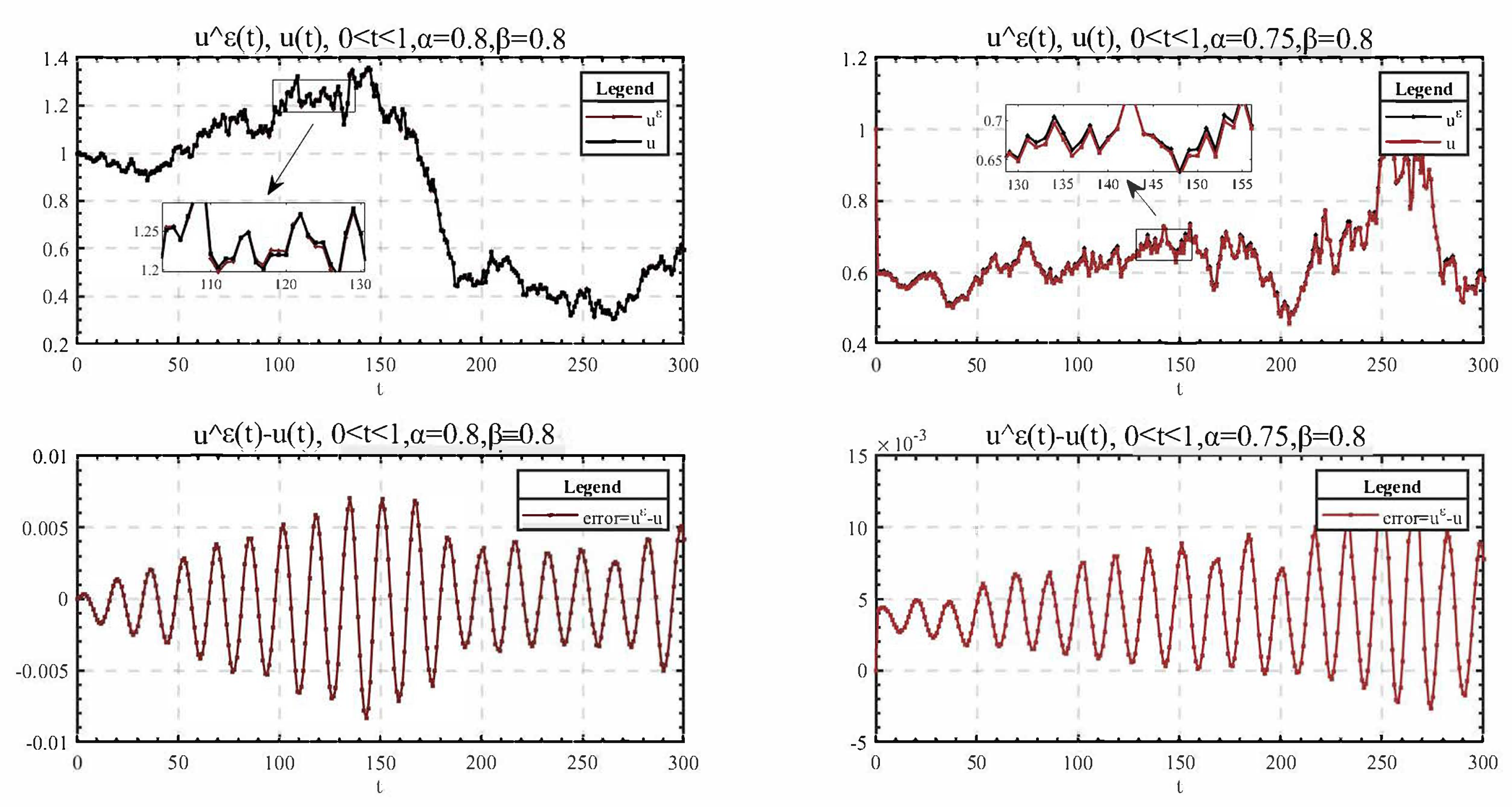
In Figure 1, we describe the approximation effect of the average value principle when $\alpha$ takes different values through numerical simulation. Figure 1 and Figure 2 may be compared to show how the value of $\epsilon$ affects how accurate an estimate is. The accuracy of the approximation increases with decreasing value of $\epsilon$.

5. Conclusions

In this study, we prove that the solution to (10) can in the sense of the mean square approximate the solution to (1). This is an averaging principle that we established for a type of time fractal–fractional differential SDE under a general averaging condition, which extended the present studies of the averaging principle for SDEs. After careful estimation, we establish an effective approximation for the solution of SDEs in a mean square. In the future, we can consider the use of fractional color noise to characterize the memorability of the system and approximate the original equation by the averaging principle to study the properties of the system conveniently.