A New L²-Gradient Flow-Based Fractional-in-Space Modified Phase-Field Crystal Equation and Its Mass Conservative and Energy Stable Method

Abstract

In this paper, we introduce a new fractional-in-space modified phase-field crystal equation based on the $L^2$-gradient flow approach, where the mass of atoms is conserved by using a nonlocal Lagrange multiplier. To solve the $L^2$-gradient flow-based fractional-in-space modified phase-field crystal equation, we present a mass conservative and energy stable method based on the convex splitting idea. Numerical examples together with standard tests in the classical $H^{-1}$-gradient flow-based modified phase-field crystal equation are provided to illustrate the applicability of the proposed framework.

1. Introduction

The modified phase-field crystal (MPFC) equation was introduced to describe both diffusive dynamics and elastic interactions [1]:

$$\begin{array}{c}\hfill \frac{{\partial }^2\varphi }{\partial t^2}+\beta \frac{\partial \varphi }{\partial t}=\mathsf{\Delta }\mu ,\mu :=\frac{\delta \mathcal{E}}{\delta \varphi }={\varphi }^3+(1-ϵ)\varphi +2\mathsf{\Delta }\varphi +{\mathsf{\Delta }}^2\varphi ,\end{array}$$

(1)

where $\varphi$ is the density field, $\beta >0$ is a constant, $\mu$ is the chemical potential, $\frac{\delta }{\delta \varphi }$ denotes the variational derivative, and $\mathcal{E}$ is the Swift–Hohenberg energy functional [2]:

$$\begin{array}{c}\hfill \mathcal{E}\left(\varphi \right):={\int }_{\mathsf{\Omega }}\left(\frac{1}{4}{\varphi }^4+\frac{1-ϵ}{2}{\varphi }^2-{|\nabla \varphi |}^2+\frac{1}{2}{\left(\mathsf{\Delta }\varphi \right)}^2\right)d\mathbf{x},\end{array}$$

(2)

where $0<ϵ<1$ is a constant with physical significance. We assume that $\varphi$ and $\mu$ are periodic on $\mathsf{\Omega }$. Note that (i) $\frac{d}{dt}{\int }_{\mathsf{\Omega }}\varphi d\mathbf{x}={\int }_{\mathsf{\Omega }}\frac{\partial \varphi }{\partial t}d\mathbf{x}=0$ if we employ an initial condition satisfying ${\int }_{\mathsf{\Omega }}\frac{\partial \varphi }{\partial t}(\mathbf{x},0)d\mathbf{x}=0$; (ii) solutions of the MPFC equation dissipate the following energy [3]:

$$\begin{array}{c}\hfill \tilde{\mathcal{E}}\left(\varphi \right):=\mathcal{E}\left(\varphi \right)+\frac{1}{2}{∥\frac{\partial \varphi }{\partial t}∥}_{H^{-1}}^2,\end{array}$$

(3)

where ${(·,·)}_{H^{-1}}$ denotes the $H^{-1}$-inner product with respect to $\mathsf{\Omega }$.

Fractional differential equations have been proved to be valuable tools for modeling diffusive processes associated with anomalous diffusion [4,5,6,7,8]. To describe superdiffusion in the MPFC model, we consider a fractional-in-space version of the MPFC equation

$$\begin{array}{c}\hfill \frac{{\partial }^2\varphi }{\partial t^2}+\beta \frac{\partial \varphi }{\partial t}=\mathsf{\Delta }{\mu }^s,{\mu }^s:=\frac{\delta {\mathcal{E}}^s}{\delta \varphi }={\varphi }^3+(1-ϵ)\varphi -2{(-\mathsf{\Delta })}^{\frac{s}{2}}\varphi +{(-\mathsf{\Delta })}^s\varphi ,\end{array}$$

(4)

where ${(-\mathsf{\Delta })}^{\frac{s}{2}}$ is the fractional Laplacian ($1<s\le 2$), and

$$\begin{array}{c}\hfill {\mathcal{E}}^s\left(\varphi \right):={\int }_{\mathsf{\Omega }}\left(\frac{1}{4}{\varphi }^4+\frac{1-ϵ}{2}{\varphi }^2-{\left|{(-\mathsf{\Delta })}^{\frac{s}{4}}\varphi \right|}^2+\frac{1}{2}{\left({(-\mathsf{\Delta })}^{\frac{s}{2}}\varphi \right)}^2\right)d\mathbf{x}.\end{array}$$

(5)

Note that the fractional-in-space MPFC equation reduces to the MPFC equation when $s=2$.

Various methods have been proposed to solve the MPFC equation [9,10,11,12,13,14,15]. In [9,12], the authors presented second-order methods based on the convex splitting idea. Galenko et al. [10] introduced a second-order method with a higher-order generalization of the trapezoidal rule. In [13], Li et al. developed second-order methods based on the invariant energy quadratization approach. Li and Shen [14] constructed a second-order method based on the scalar auxiliary variable approach. In [15], Shin et al. presented high-order (up to fourth-order) methods by combining the concept of energy quadratization and the Runge–Kutta method. Note that the MPFC equation needs to discretize the linear sixth-order, nonlinear second-order, and inverse Laplacian terms.

The aim of this paper is to reformulate the fractional-in-space MPFC equation through the variational approach in the $L^2$-space, where a nonlocal Lagrange multiplier is added to cancel out the variation of mass without influencing the energy dissipation property. Then, the new $L^2$-gradient flow-based fractional-in-space MPFC ($L^2$-fMPFC) equation only needs to discretize the linear fourth-order and nonlinear terms. To solve the $L^2$-fMPFC equation with preserving the mass conservation and energy stability, we propose a numerical method by applying a convex splitting to both the $L^2$-gradient flow and nonlocal terms. In addition, to have second-order time accuracy, the convex and concave parts are treated using a second-order secant type approach and a second-order extrapolation, respectively. We prove that the method is mass conservative, unconditionally uniquely solvable, and unconditionally stable with respect to the energy of the $L^2$-fMPFC equation.

The organization of this paper is as follows. In Section 2, we introduce the $L^2$-fMPFC equation and its energy. In Section 3, we develop the second-order method for the $L^2$-fMPFC equation and give proofs of its mass conservation, unconditional unique solvability, and unconditional energy stability. In Section 4, we provide numerical examples illustrating the applicability of the proposed framework. Finally, conclusions are drawn in Section 5.

2. ${\mathit{L}}^{\mathbf{2}}$-Gradient Flow-Based Fractional-In-Space Modified Phase-Field Crystal Equation

We introduce the new $L^2$-fMPFC equation:

$$\begin{array}{c}\hfill \frac{{\partial }^2\varphi }{\partial t^2}+\beta \frac{\partial \varphi }{\partial t}=-{\mu }^s+\alpha \left(t\right),\end{array}$$

(6)

where $\alpha \left(t\right)=\frac{1}{\left|\mathsf{\Omega }\right|}{\int }_{\mathsf{\Omega }}{\mu }^{s}d\mathbf{x}$ is the nonlocal Lagrange multiplier. In addition, we introduce the energy:

$$\begin{array}{c}\hfill \mathcal{F}\left(\varphi \right):={\mathcal{E}}^s\left(\varphi \right)+\frac{1}{2}{∥\frac{\partial \varphi }{\partial t}∥}_{L^2}^2,\end{array}$$

(7)

where ${(·,·)}_{L^2}$ denotes the $L^2$-inner product with respect to $\mathsf{\Omega }$.

Integrating Equation (6) over $\mathsf{\Omega }$ and letting $\mathsf{\Psi }\left(t\right)={\int }_{\mathsf{\Omega }}\frac{\partial \varphi }{\partial t}d\mathbf{x}$, we obtain

$$\begin{array}{c}\hfill \frac{d\mathsf{\Psi }\left(t\right)}{dt}+\beta \mathsf{\Psi }\left(t\right)=-{\int }_{\mathsf{\Omega }}{\mu }^{s}d\mathbf{x}+{\int }_{\mathsf{\Omega }}{\mu }^{s}d\mathbf{x}=0.\end{array}$$

A solution of this equation is $\mathsf{\Psi }\left(t\right)=\mathsf{\Psi }\left(0\right)e^{-\beta t}$. Thus, if we employ an initial condition satisfying $\mathsf{\Psi }\left(0\right)=0$, then

$$\begin{array}{c}\hfill \mathsf{\Psi }\left(t\right)=0,t\ge 0.\end{array}$$

The energy $\mathcal{F}\left(\varphi \right)$ is nonincreasing in time:

$$\begin{array}{ccc}\hfill \frac{d\mathcal{F}}{dt}& =& {\left({\mu }^s,\frac{\partial \varphi }{\partial t}\right)}_{L^2}+{\left(\frac{\partial \varphi }{\partial t},\frac{{\partial }^2\varphi }{\partial t^2}\right)}_{L^2}={\left(\frac{\partial \varphi }{\partial t},-\beta \frac{\partial \varphi }{\partial t}+\alpha \left(t\right)\right)}_{L^2}\hfill \\ & =& -\beta {∥\frac{\partial \varphi }{\partial t}∥}_{L^2}^2+\alpha \left(t\right)\mathsf{\Psi }\left(t\right)=-\beta {∥\frac{\partial \varphi }{\partial t}∥}_{L^2}^2\le 0.\hfill \end{array}$$

3. Mass Conservative and Energy Stable Method

Using a new variable $\psi$, Equation (6) can be split as

$$\begin{array}{ccc}\hfill \frac{\partial \psi }{\partial t}& =& -{\mu }^s+\alpha \left(t\right)-\beta \psi ,\hfill \end{array}$$

(8)

$$\begin{array}{ccc}\hfill \frac{\partial \varphi }{\partial t}& =& \psi \hfill \end{array}$$

(9)

and the energy $\mathcal{F}\left(\varphi \right)$ can be redefined as

$$\begin{array}{c}\hfill \mathcal{F}(\varphi ,\psi ):={\mathcal{E}}^s\left(\varphi \right)+\frac{1}{2}{∥\psi ∥}_{L^2}^2.\end{array}$$

(10)

Then, Equations (8) and (9) can be discretized with second-order time accuracy as follows:

$$\begin{array}{ccc}\hfill \frac{{\psi }^{n+1}-{\psi }^n}{\mathsf{\Delta }t}& =& -{\mu }^{s,n+\frac{1}{2}}+{\alpha }^{n+\frac{1}{2}}-\beta \frac{{\psi }^{n+1}+{\psi }^n}{2},\hfill \end{array}$$

(11)

$$\begin{array}{ccc}\hfill {\mu }^{s,n+\frac{1}{2}}& =& \chi ({\varphi }^{n+1},{\varphi }^n)+{(-\mathsf{\Delta })}^s\left(\frac{{\varphi }^{n+1}+{\varphi }^n}{2}\right)-{(-\mathsf{\Delta })}^{\frac{s}{2}}(3{\varphi }^n-{\varphi }^{n-1}),\hfill \end{array}$$

(12)

$$\begin{array}{ccc}\hfill \frac{{\varphi }^{n+1}-{\varphi }^n}{\mathsf{\Delta }t}& =& \frac{{\psi }^{n+1}+{\psi }^n}{2},\hfill \end{array}$$

(13)

where $\chi (\varphi ,\phi )=\frac{{\varphi }^2+{\phi }^2}{2}\frac{\varphi +\phi }{2}+(1-ϵ)\frac{\varphi +\phi }{2}$, ${\alpha }^{n+\frac{1}{2}}=\frac{1}{\left|\mathsf{\Omega }\right|}{\left({\mu }^{s,n+\frac{1}{2}},\mathbf{1}\right)}_{L^2}$, and ${\varphi }^{-1}\equiv {\varphi }^0$. Note that we discretize ${\mu }^{s,n+\frac{1}{2}}$ and ${\alpha }^{n+\frac{1}{2}}$ based on the following convex splitting of the energy ${\mathcal{E}}^s\left(\varphi \right)$ [16]:

$$\begin{array}{c}\hfill {\mathcal{E}}^s\left(\varphi \right)={\mathcal{E}}_c^s\left(\varphi \right)-{\mathcal{E}}_e^s\left(\varphi \right)={\int }_{\mathsf{\Omega }}\left(\frac{1}{4}{\varphi }^4+\frac{1-ϵ}{2}{\varphi }^2+\frac{1}{2}{\left({(-\mathsf{\Delta })}^{\frac{s}{2}}\varphi \right)}^2\right)d\mathbf{x}-{\int }_{\mathsf{\Omega }}{\left|{(-\mathsf{\Delta })}^{\frac{s}{4}}\varphi \right|}^{2}d\mathbf{x}.\end{array}$$

Theorem 1.

The second-order method (11)–(13) with an initial condition satisfying Ψ(0) = 0 is mass conservative.

Proof. 

From Equation (11), we obtain

$$\begin{array}{ccc}\hfill {({\psi }^{n+1}-{\psi }^n,\mathbf{1})}_{L^2}& =& \mathsf{\Delta }t{(-{\mu }^{s,n+\frac{1}{2}}+{\alpha }^{n+\frac{1}{2}},\mathbf{1})}_{L^2}-\frac{\beta \mathsf{\Delta }t}{2}{({\psi }^{n+1}+{\psi }^n,\mathbf{1})}_{L^2}\hfill \\ & =& -\frac{\beta \mathsf{\Delta }t}{2}{({\psi }^{n+1}+{\psi }^n,\mathbf{1})}_{L^2}.\hfill \end{array}$$

This yields the relation

$$\begin{array}{c}\hfill {({\psi }^{n+1},\mathbf{1})}_{L^2}=\frac{2-\beta \mathsf{\Delta }t}{2+\beta \mathsf{\Delta }t}{({\psi }^n,\mathbf{1})}_{L^2}.\end{array}$$

With an initial condition satisfying $\mathsf{\Psi }\left(0\right)=0$, i.e., ${({\psi }^0,\mathbf{1})}_{L^2}=0$, the relation guarantees that ${({\psi }^{n+1},\mathbf{1})}_{L^2}=0$ for all $n\ge 0$. Now, from Equation (13), we see that

$$\begin{array}{c}\hfill {({\varphi }^{n+1}-{\varphi }^n,\mathbf{1})}_{L^2}=0\mathrm{if}\mathrm{and}\mathrm{only}\mathrm{if}{({\psi }^{n+1},\mathbf{1})}_{L^2}=0,\end{array}$$

and the result follows: ${({\varphi }^{n+1},\mathbf{1})}_{L^2}={({\varphi }^n,\mathbf{1})}_{L^2}$. □

Before proving the unique solvability of the second-order method (11)–(13), we simplify the method as follows:

$$\begin{array}{ccc}\hfill \frac{{\varphi }^{n+1}-{\varphi }^n}{\mathsf{\Delta }t}& =& -\frac{\mathsf{\Delta }t}{2+\beta \mathsf{\Delta }t}\left({\mu }^{s,n+\frac{1}{2}}-{\alpha }^{n+\frac{1}{2}}\right)+\frac{2}{2+\beta \mathsf{\Delta }t}{\psi }^n,\hfill \end{array}$$

(14)

$$\begin{array}{ccc}\hfill {\psi }^{n+1}& =& 2\frac{{\varphi }^{n+1}-{\varphi }^n}{\mathsf{\Delta }t}-{\psi }^n.\hfill \end{array}$$

(15)

Theorem 2.

The second-order method (12) and (14)–(15) with an initial condition satisfying Ψ(0) = 0 is unconditionally uniquely solvable.

Proof. 

We consider the following functional for $\varphi$ defined in the constraint space ${(\varphi ,\mathbf{1})}_{L^2}={({\varphi }^n,\mathbf{1})}_{L^2}$ given by Theorem 1:

$$\begin{array}{c}\hfill G\left(\varphi \right)=\frac{1}{2\mathsf{\Delta }t}{\parallel \varphi -{\varphi }^n\parallel }_{L^2}^2+\frac{\mathsf{\Delta }t}{2+\beta \mathsf{\Delta }t}H\left(\varphi \right)-\frac{2}{2+\beta \mathsf{\Delta }t}{({\psi }^n,\varphi )}_{L^2},\end{array}$$

where

$$\begin{array}{ccc}\hfill H\left(\varphi \right)& =& \frac{1}{4}{\left(\frac{{\varphi }^4}{4}+\frac{{\varphi }^3}{3}{\varphi }^n+\frac{{\varphi }^2}{2}{\left({\varphi }^n\right)}^2+\varphi {\left({\varphi }^n\right)}^3,\mathbf{1}\right)}_{L^2}+\frac{1-ϵ}{2}{\left(\frac{{\varphi }^2}{2}+\varphi {\varphi }^n,\mathbf{1}\right)}_{L^2}\hfill \\ & & +\frac{1}{4}{\parallel {(-\mathsf{\Delta })}^{\frac{s}{2}}\varphi \parallel }_{L^2}^2+{\left(\frac{1}{2}{(-\mathsf{\Delta })}^s{\varphi }^n-{(-\mathsf{\Delta })}^{\frac{s}{2}}(3{\varphi }^n-{\varphi }^{n-1}),\varphi \right)}_{L^2}.\hfill \end{array}$$

It may be shown that ${\varphi }^{n+1}$ is the unique minimizer of $G\left(\varphi \right)$ if and only if it solves, for any $\phi$ with ${(\phi ,\mathbf{1})}_{L^2}=0$,

$$\begin{array}{ccc}\hfill {\left.\frac{dG(\varphi +\eta \phi )}{d\eta }\right|}_{\eta =0}& =& {\left(\frac{\varphi -{\varphi }^n}{\mathsf{\Delta }t},\phi \right)}_{L^2}+\frac{\mathsf{\Delta }t}{2+\beta \mathsf{\Delta }t}{\left(\chi (\varphi ,{\varphi }^n)+\frac{1}{2}{(-\mathsf{\Delta })}^s\varphi ,\phi \right)}_{L^2}\hfill \\ & & +\frac{\mathsf{\Delta }t}{2+\beta \mathsf{\Delta }t}{\left(\frac{1}{2}{(-\mathsf{\Delta })}^s{\varphi }^n-{(-\mathsf{\Delta })}^{\frac{s}{2}}(3{\varphi }^n-{\varphi }^{n-1}),\phi \right)}_{L^2}\hfill \\ & & -\frac{2}{2+\beta \mathsf{\Delta }t}{({\psi }^n,\phi )}_{L^2}=0,\hfill \end{array}$$

(16)

because $G\left(\varphi \right)$ is strictly convex by

$$\begin{array}{ccc}\hfill {\left.\frac{d^{2}G(\varphi +\eta \phi )}{d{\eta }^2}\right|}_{\eta =0}& =& \frac{1}{\mathsf{\Delta }t}{\parallel \phi \parallel }_{L^2}^2+\frac{\mathsf{\Delta }t}{2+\beta \mathsf{\Delta }t}{\left(\frac{{\varphi }^2}{2}+\frac{1}{4}{(\varphi +{\varphi }^n)}^2+\frac{1-ϵ}{2},{\phi }^2\right)}_{L^2}\hfill \\ & & +\frac{\mathsf{\Delta }t}{2(2+\beta \mathsf{\Delta }t)}{\parallel {(-\mathsf{\Delta })}^{\frac{s}{2}}\phi \parallel }_{L^2}^2\ge 0.\hfill \end{array}$$

Since 1 is in the null space of the inner product with $\phi$, the solution of (16) can be rewritten as follows:

$$\begin{array}{c}\hfill \frac{\varphi -{\varphi }^n}{\mathsf{\Delta }t}=-\frac{\mathsf{\Delta }t}{2+\beta \mathsf{\Delta }t}\left(\chi (\varphi ,{\varphi }^n)+{(-\mathsf{\Delta })}^s\left(\frac{\varphi +{\varphi }^n}{2}\right)-{(-\mathsf{\Delta })}^{\frac{s}{2}}(3{\varphi }^n-{\varphi }^{n-1})\right)+\frac{2}{2+\beta \mathsf{\Delta }t}{\psi }^n+\mathsf{\Lambda }\mathbf{1}.\end{array}$$

Using the constraint ${(\varphi ,\mathbf{1})}_{L^2}={({\varphi }^n,\mathbf{1})}_{L^2}$ and ${({\psi }^n,\mathbf{1})}_{L^2}=0$ given by Theorem 1, we have $\mathsf{\Lambda }=\frac{\mathsf{\Delta }t}{(2+\beta \mathsf{\Delta }t)\left|\mathsf{\Omega }\right|}{\left(\chi (\varphi ,{\varphi }^n)+{(-\mathsf{\Delta })}^s\left(\frac{\varphi +{\varphi }^n}{2}\right)-{(-\mathsf{\Delta })}^{\frac{s}{2}}(3{\varphi }^n-{\varphi }^{n-1}),\mathbf{1}\right)}_{L^2}$, which concludes the proof. □

Theorem 3.

The second-order method (12) and (14)–(15) with an initial condition satisfying Ψ(0) = 0 is unconditionally energy stable,

$$\begin{array}{c}\hfill \tilde{\mathcal{F}}({\varphi }^{n+1},{\psi }^{n+1},{\varphi }^n)\le \tilde{\mathcal{F}}({\varphi }^n,{\psi }^n,{\varphi }^{n-1}),\end{array}$$

where

$$\begin{array}{c}\hfill \tilde{\mathcal{F}}(\varphi ,\psi ,\phi ):=\mathcal{F}(\varphi ,\psi )+\frac{1}{2}{\parallel {(-\mathsf{\Delta })}^{\frac{s}{4}}(\varphi -\phi )\parallel }_{L^2}^2.\end{array}$$

Proof. 

Adding the identities

$$\begin{array}{ccc}& & {\left({\varphi }^{n+1}-{\varphi }^n,\chi ({\varphi }^{n+1},{\varphi }^n)+{(-\mathsf{\Delta })}^s\left(\frac{{\varphi }^{n+1}+{\varphi }^n}{2}\right)\right)}_{L^2}\hfill \\ & & ={\mathcal{E}}^s\left({\varphi }^{n+1}\right)-{\mathcal{E}}^s\left({\varphi }^n\right)+\parallel {(-\mathsf{\Delta })}^{\frac{s}{4}}{\varphi }^{n+1}{\parallel }_{L^2}^2-{\parallel {(-\mathsf{\Delta })}^{\frac{s}{4}}{\varphi }^n\parallel }_{L^2}^2\hfill \end{array}$$

and

$$\begin{array}{ccc}& & {\left({\varphi }^{n+1}-{\varphi }^n,-{(-\mathsf{\Delta })}^{\frac{s}{2}}(3{\varphi }^n-{\varphi }^{n-1})\right)}_{L^2}{+\parallel (-\mathsf{\Delta })}^{\frac{s}{4}}{\varphi }^{n+1}{\parallel }_{L^2}^2-{\parallel {(-\mathsf{\Delta })}^{\frac{s}{4}}{\varphi }^n\parallel }_{L^2}^2\hfill \\ & & =\frac{1}{2}{\parallel (-\mathsf{\Delta })}^{\frac{s}{4}}({\varphi }^{n+1}-{\varphi }^n){\parallel }_{L^2}^2-\frac{1}{2}{\parallel {(-\mathsf{\Delta })}^{\frac{s}{4}}({\varphi }^n-{\varphi }^{n-1})\parallel }_{L^2}^2\hfill \\ & & +\frac{1}{2}{\parallel {(-\mathsf{\Delta })}^{\frac{s}{4}}({\varphi }^{n+1}-2{\varphi }^n+{\varphi }^{n-1})\parallel }_{L^2}^2,\hfill \end{array}$$

we have from Equations (12) and (15)

$$\begin{array}{ccc}& & {(\mathsf{\Delta }t{\psi }^{n+\frac{1}{2}},{\mu }^{s,n+\frac{1}{2}})}_{L^2}={({\varphi }^{n+1}-{\varphi }^n,{\mu }^{s,n+\frac{1}{2}})}_{L^2}\hfill \\ & & ={\mathcal{E}}^s\left({\varphi }^{n+1}\right)+\frac{1}{2}\parallel {(-\mathsf{\Delta })}^{\frac{s}{4}}({\varphi }^{n+1}-{\varphi }^n){\parallel }_{L^2}^2-{\mathcal{E}}^s\left({\varphi }^n\right)-\frac{1}{2}{\parallel {(-\mathsf{\Delta })}^{\frac{s}{4}}({\varphi }^n-{\varphi }^{n-1})\parallel }_{L^2}^2\hfill \\ & & +\frac{1}{2}{\parallel {(-\mathsf{\Delta })}^{\frac{s}{4}}({\varphi }^{n+1}-2{\varphi }^n+{\varphi }^{n-1})\parallel }_{L^2}^2,\hfill \end{array}$$

where ${\psi }^{n+\frac{1}{2}}=\frac{{\psi }^{n+1}+{\psi }^n}{2}$. In addition, we obtain from Equation (14) and Theorem 1

$$\begin{array}{ccc}\hfill {({\psi }^{n+\frac{1}{2}},-\mathsf{\Delta }t{\mu }^{s,n+\frac{1}{2}})}_{L^2}& =& {\left({\psi }^{n+\frac{1}{2}},{\psi }^{n+1}-{\psi }^n-\mathsf{\Delta }t{\alpha }^{n+\frac{1}{2}}+\beta \mathsf{\Delta }t{\psi }^{n+\frac{1}{2}}\right)}_{L^2}\hfill \\ & =& \frac{1}{2}\parallel {\psi }^{n+1}{\parallel }_{L^2}^2-\frac{1}{2}\parallel {\psi }^n{\parallel }_{L^2}^2-\mathsf{\Delta }t{\alpha }^{n+\frac{1}{2}}{({\psi }^{n+\frac{1}{2}},\mathbf{1})}_{L^2}+\beta \mathsf{\Delta }t{\parallel {\psi }^{n+\frac{1}{2}}\parallel }_{L^2}^2\hfill \\ & =& \frac{1}{2}\parallel {\psi }^{n+1}{\parallel }_{L^2}^2-\frac{1}{2}\parallel {\psi }^n{\parallel }_{L^2}^2+\beta \mathsf{\Delta }t{\parallel {\psi }^{n+\frac{1}{2}}\parallel }_{L^2}^2.\hfill \end{array}$$

Then, we have

$$\begin{array}{ccc}& & \tilde{\mathcal{F}}({\varphi }^{n+1},{\psi }^{n+1},{\varphi }^n)-\tilde{\mathcal{F}}({\varphi }^n,{\psi }^n,{\varphi }^{n-1})\hfill \\ & & =-\beta \mathsf{\Delta }t\parallel {\psi }^{n+\frac{1}{2}}{\parallel }_{L^2}^2-\frac{1}{2}{\parallel {(-\mathsf{\Delta })}^{\frac{s}{4}}({\varphi }^{n+1}-2{\varphi }^n+{\varphi }^{n-1})\parallel }_{L^2}^2\le 0.\hfill \end{array}$$

□

Numerical Implementation

To handle ${\left({\varphi }^{n+1}\right)}^3$ and ${\left({\varphi }^{n+1}\right)}^2$ in ${\mu }^{s,n+\frac{1}{2}}$ and ${\alpha }^{n+\frac{1}{2}}$ in Equation (14), a Newton-type linearization is used [9,12,17]:

$$\begin{array}{ccc}\hfill {\left({\varphi }^{n,m+1}\right)}^3& \approx & {\left({\varphi }^{n,m}\right)}^3+3{\left({\varphi }^{n,m}\right)}^2({\varphi }^{n,m+1}-{\varphi }^{n,m}),\hfill \\ \hfill {\left({\varphi }^{n,m+1}\right)}^2& \approx & {\left({\varphi }^{n,m}\right)}^2+2{\varphi }^{n,m}({\varphi }^{n,m+1}-{\varphi }^{n,m})\hfill \end{array}$$

for $m=0,1,\dots$. We then develop a Newton-type fixed point iteration method for Equation (14) starting with ${\varphi }^{n,0}={\varphi }^n$ as

$$\begin{array}{ccc}& & \left[I+\frac{\mathsf{\Delta }{t}^2}{2+\beta \mathsf{\Delta }t}\left(A^{n,m}+\frac{1}{2}{(-\mathsf{\Delta })}^s-\frac{1}{\left|\mathsf{\Omega }\right|}{\left(A^{n,m},·\right)}_{L^2}\right)\right]{\varphi }^{n,m+1}\hfill \\ & & ={\varphi }^n-\frac{\mathsf{\Delta }{t}^2}{2+\beta \mathsf{\Delta }t}\left(B^{n,m}+\frac{1}{2}{(-\mathsf{\Delta })}^s{\varphi }^n-{(-\mathsf{\Delta })}^{\frac{s}{2}}(3{\varphi }^n-{\varphi }^{n-1})-\frac{1}{\left|\mathsf{\Omega }\right|}{\left(B^{n,m},\mathbf{1}\right)}_{L^2}\right)\hfill \\ & & +\frac{2\mathsf{\Delta }t}{2+\beta \mathsf{\Delta }t}{\psi }^n,\hfill \end{array}$$

(17)

where $A^{n,m}=\frac{3{\left({\varphi }^{n,m}\right)}^2+2{\varphi }^{n,m}{\varphi }^n+{\left({\varphi }^n\right)}^2}{4}+\frac{1-ϵ}{2}$, ${\left(A^{n,m},·\right)}_{L^2}\varphi ={\left(A^{n,m},\varphi \right)}_{L^2}$,

$B^{n,m}=\frac{-2{\left({\varphi }^{n,m}\right)}^3-{\left({\varphi }^{n,m}\right)}^2{\varphi }^n+{\left({\varphi }^n\right)}^3}{4}+\frac{1-ϵ}{2}{\varphi }^n$, and we set

$$\begin{array}{c}\hfill {\varphi }^{n+1}={\varphi }^{n,m+1}\end{array}$$

if a relative $l_2$-norm of the consecutive error $\frac{{∥{\varphi }^{n,m+1}-{\varphi }^{n,m}∥}_2}{{∥{\varphi }^{n,m}∥}_2}$ is less than a tolerance $tol$.

The system (17) is solved using the biconjugate gradient method with the preconditioner $P=I+\frac{\mathsf{\Delta }{t}^2}{2(2+\beta \mathsf{\Delta }t)}{(-\mathsf{\Delta })}^s$. The stopping criterion for the biconjugate gradient iteration is that the relative residual norm is less than $tol$. Then, we employ the Fourier spectral method [15,18,19,20,21,22] for the spatial discretization, which gives a full diagonal representation of the fractional operator.

4. Numerical Experiments

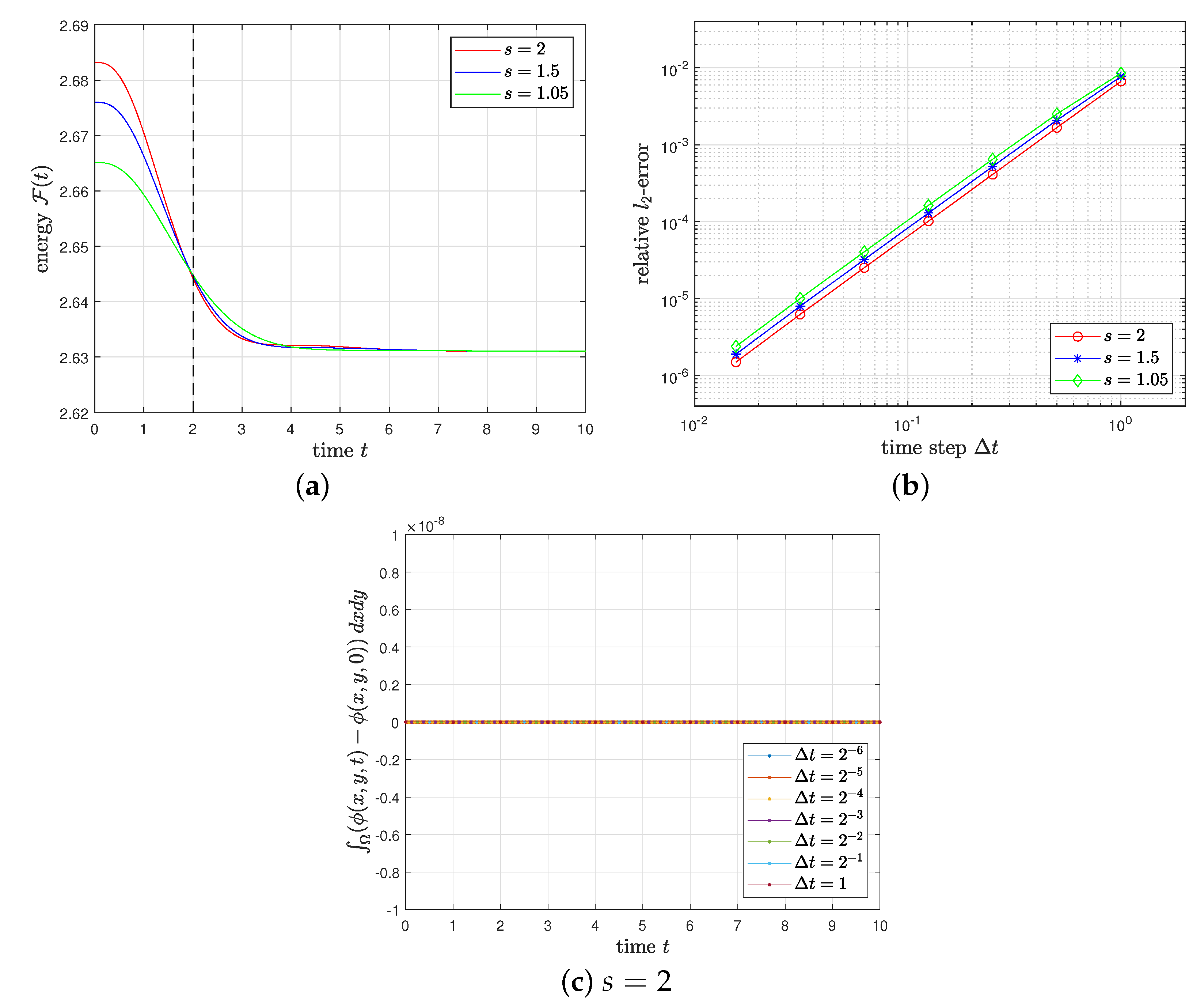
4.1. Accuracy Test

We estimate the accuracy of the proposed method with initial conditions [17]

$$\begin{array}{ccc}\hfill \varphi (x,y,0)& =& 0.02{cos}^2\left(\frac{\pi (x+10)}{32}\right){sin}^2\left(\frac{\pi (y+3)}{32}\right)-0.01{sin}^2\left(\frac{\pi x}{8}\right){sin}^2\left(\frac{\pi (y-6)}{8}\right)\hfill \\ & & -0.02cos\left(\frac{\pi (x-12)}{16}\right)sin\left(\frac{\pi (y-1)}{16}\right)+0.07,\psi (x,y,0)=0\hfill \end{array}$$

(18)

on $\mathsf{\Omega }=[0,32]\times [0,32]$. We set $ϵ=0.025$, $\beta =1$, $\mathsf{\Delta }x=\mathsf{\Delta }y=\frac{1}{3}$, and $tol={10}^{-8}\mathsf{\Delta }t$, and we compute $\varphi (x,y,t)$ for $0<t\le 10$. For $s=2,1.5,1.05$, Figure 1a,b show the evolution of $\mathcal{F}\left(t\right)$ for the reference solution with $\mathsf{\Delta }t=2^{-8}$ and the relative $l_2$-errors of $\varphi (x,y,2)$ for $\mathsf{\Delta }t=2^{-6},2^{-5},\dots ,1$, respectively. Here, the errors are computed by comparison with the reference solution. Figure 1c shows the evolution of ${\int }_{\mathsf{\Omega }}(\varphi (x,y,t)-\varphi (x,y,0))dxdy$ for $s=2$ and various time steps. It is observed that the method is second-order accurate in time and conserves the mass.

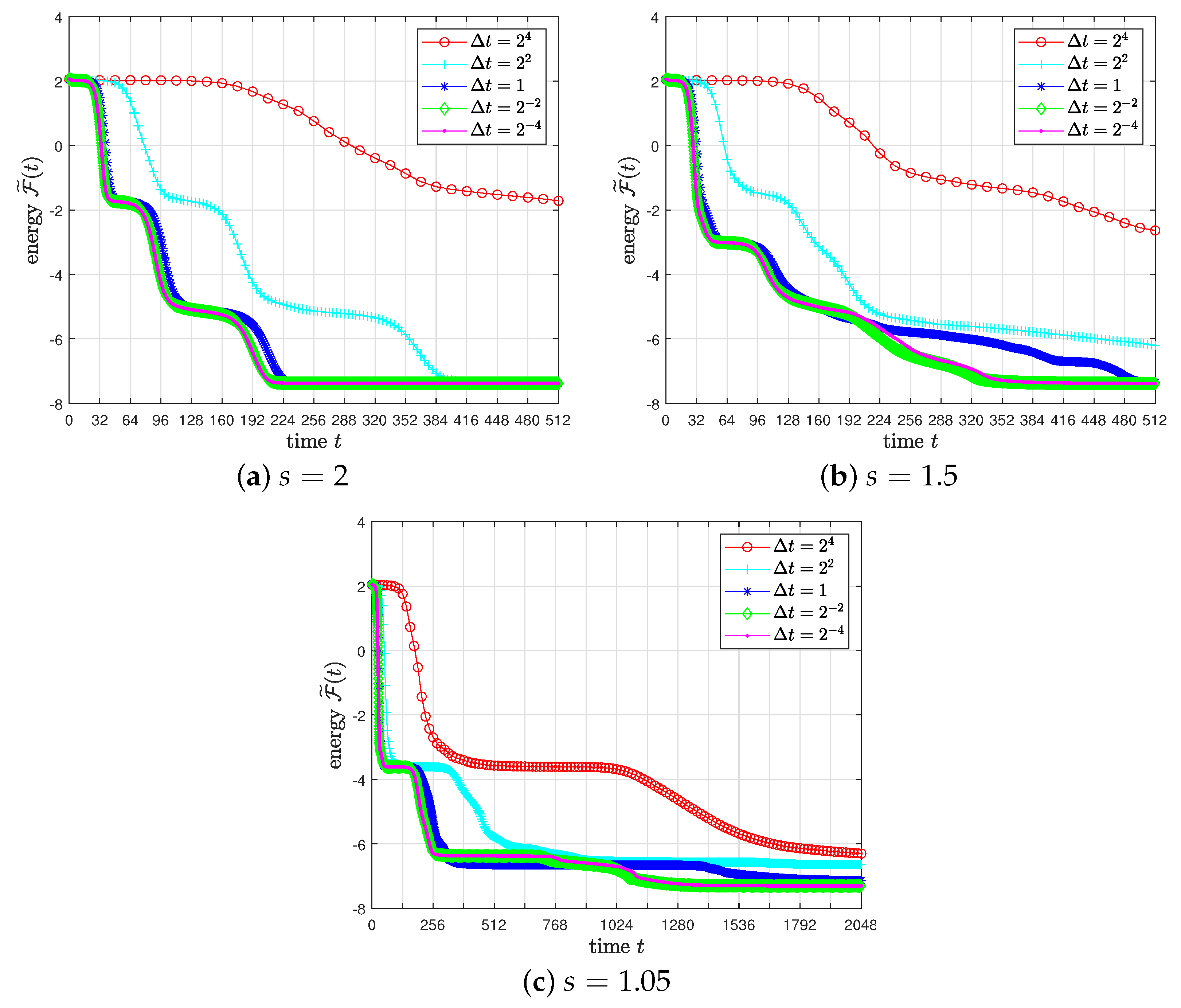
4.2. Energy Stability Test

To demonstrate the energy stability of the proposed method, we take the initial conditions (18) on $\mathsf{\Omega }=[0,32]\times [0,32]$, and use $ϵ=0.25$, $\beta =1$, $\mathsf{\Delta }x=\mathsf{\Delta }y=\frac{1}{3}$, and $tol={10}^{-8}$. For $s=2,1.5,1.05$, Figure 2a–c show the evolution of $\tilde{\mathcal{F}}\left(t\right)$ with different time steps, respectively. The energy curves are all nonincreasing in time, which verifies that the proposed method is unconditionally energy stable (Theorem 3). Moreover, the solution with $s=2$ and a sufficiently small time step $\mathsf{\Delta }t=2^{-4}$ is stable at around $t=224$ (see the magenta line with dots in Figure 2a); however, the case of $s=1.05$ is not stable even at $t=512$ (see the magenta line with dots in Figure 2c). These results show that the lifetime of the unstable interface is prolonged as the fractional order s decreases, i.e., a longer time computation is needed to reach a steady state. Figure 3 shows the evolution of $\varphi (x,y,t)$ with $s=2$ and $\mathsf{\Delta }t=2^{-4}$.

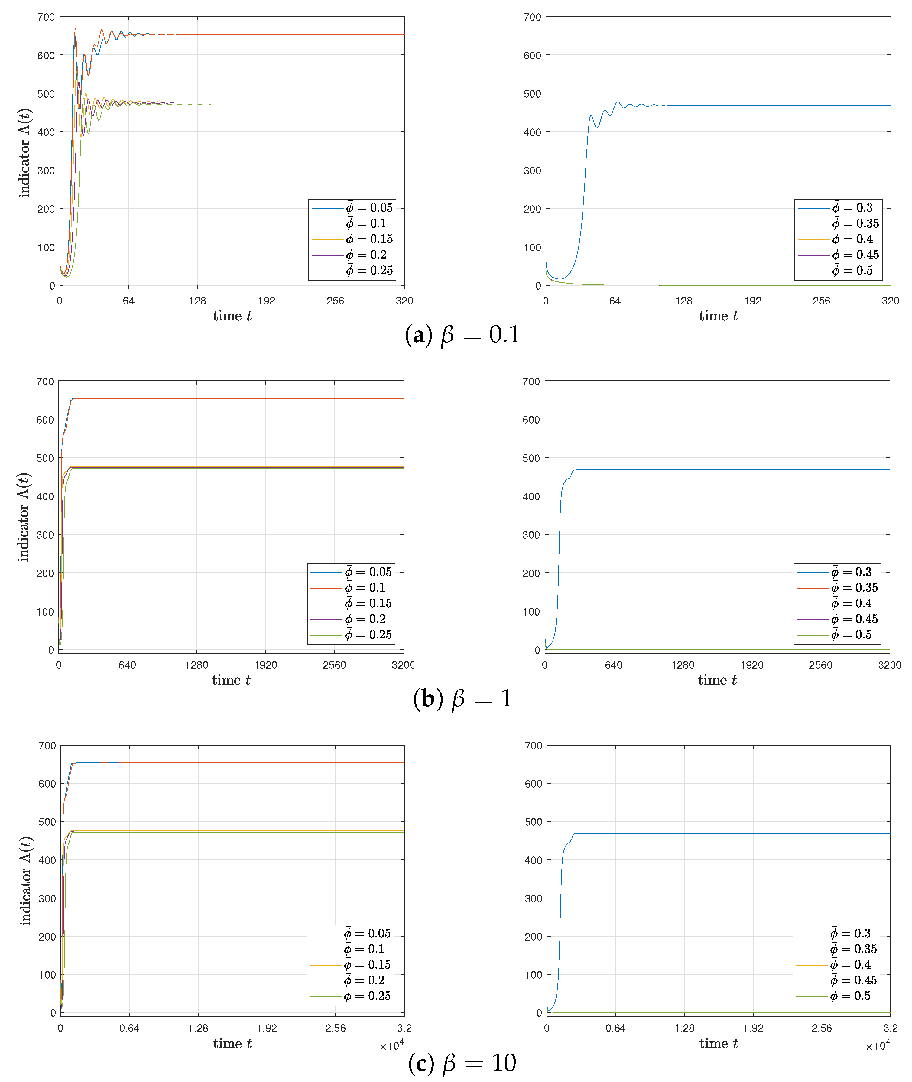
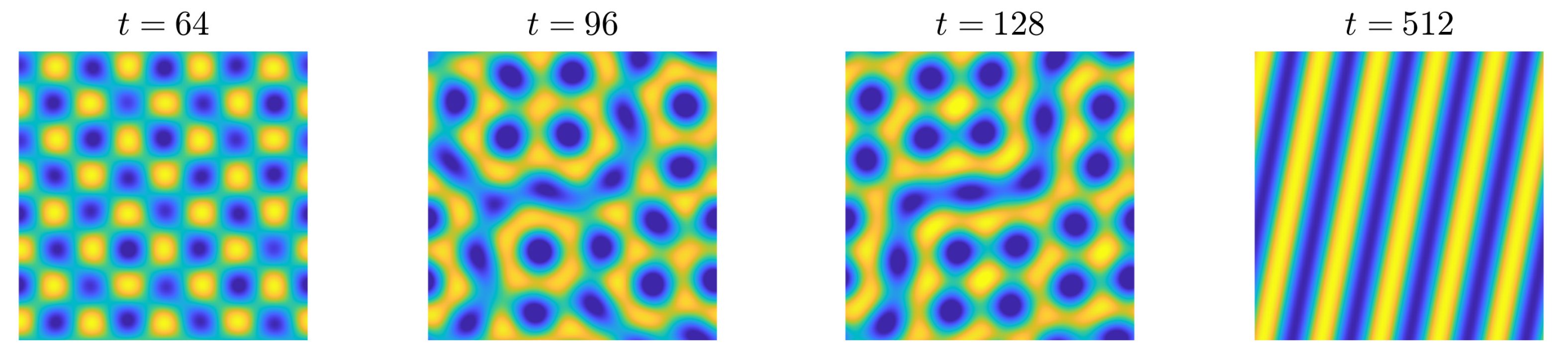
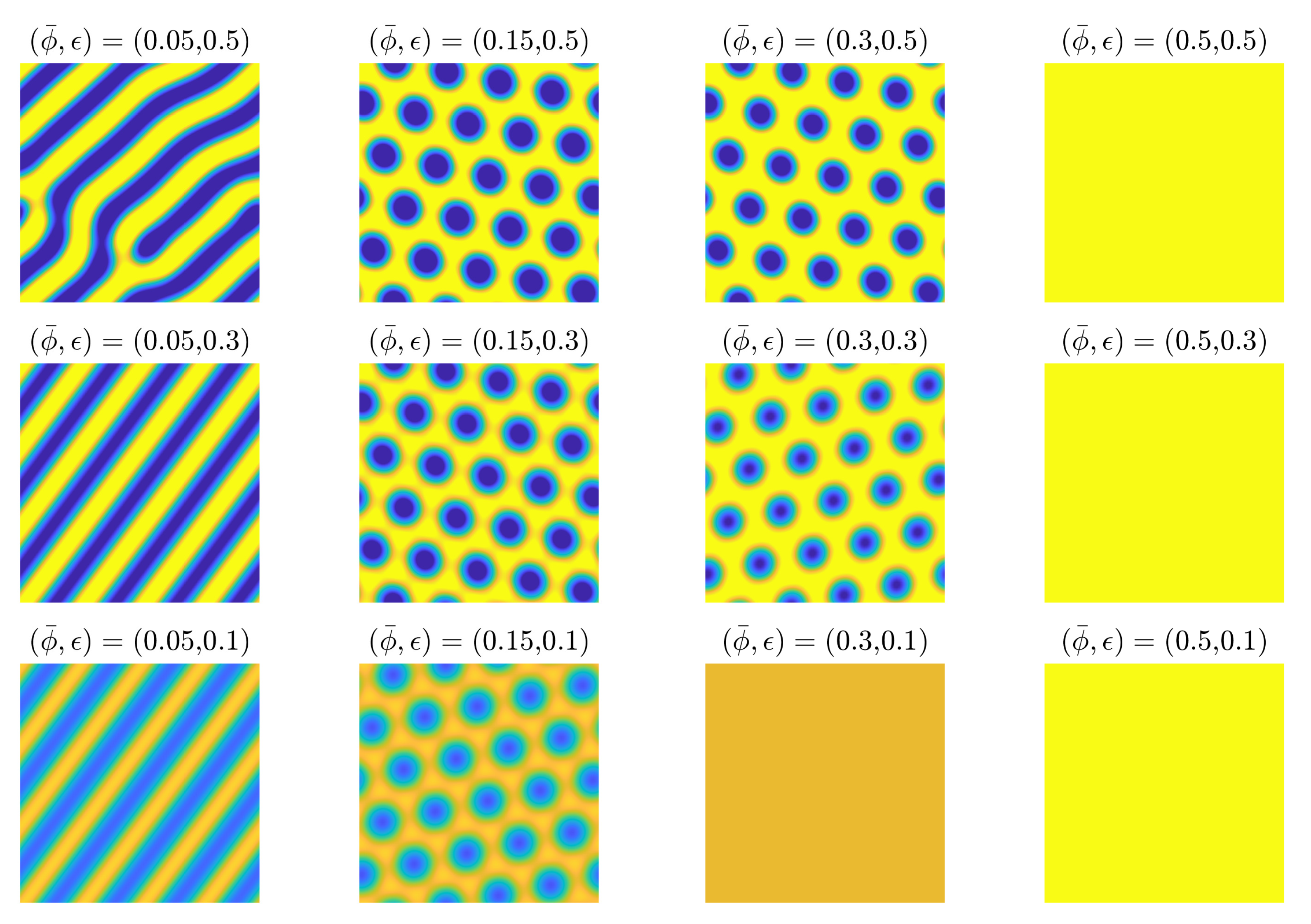
4.3. Phase Diagram in 2D

In 2D, the phase diagram contains constant (${\varphi }_c$), striped (${\varphi }_s$), and triangular (${\varphi }_t$) states depending on the values of $\overline{\varphi }$ (the average density) and $ϵ$, and these states can be approximated by ${\varphi }_c=\overline{\varphi }$, ${\varphi }_s=\overline{\varphi }+A_{s}sin\left(x\right)$, and ${\varphi }_t=\overline{\varphi }+A_t\left(cos\left(\frac{\sqrt{3}x}{2}\right)cos\left(\frac{y}{2}\right)-\frac{1}{2}cos\left(y\right)\right)$, where $A_s$ and $A_t$ are the characteristic amplitudes [23]. To verify that the proposed method does lead to the expected states, we take the initial conditions as $\varphi (x,y,0)=\overline{\varphi }+\mathrm{rand}$, $\psi (x,y,0)=0$ on $\mathsf{\Omega }=[0,32]\times [0,32]$, where rand is a random number between $-0.1$ and $0.1$ at the grid points. We use $s=2$, $\mathsf{\Delta }x=\mathsf{\Delta }y=\frac{1}{3}$, $\mathsf{\Delta }t=\frac{1}{4}\beta$, and $tol={10}^{-9}\beta$, and we compute $\varphi (x,y,t)$ for $0<t\le t_f=3200\beta$. To estimate the phase diagram numerically, we calculate the following indicator function:

$$\begin{array}{c}\hfill \mathsf{\Lambda }\left(t\right)=\left\{\begin{array}{cc}{\int }_{\mathsf{\Omega }}|\varphi (\mathbf{x},t)-\overline{\varphi }|d\mathbf{x}\hfill & \mathrm{if}A=0,\hfill \\ \frac{1}{A}{\int }_{\mathsf{\Omega }}|\varphi (\mathbf{x},t)-\overline{\varphi }|d\mathbf{x}\hfill & \mathrm{if}A\ne 0,\hfill \end{array}\right.\end{array}$$

(19)

where ${\displaystyle A=\frac{1}{2}\left(\underset{\mathbf{x}\in \mathsf{\Omega }}{max}\varphi (\mathbf{x},t_f)-\underset{\mathbf{x}\in \mathsf{\Omega }}{min}\varphi (\mathbf{x},t_f)\right)}$. In the numerical simulations, we set $A=0$ if A is less than ${10}^{-8}$. Figure 4a–c show $\mathsf{\Lambda }\left(t\right)$ at $t=t_f$ with various $\overline{\varphi }=0.05,0.1,\dots ,0.5$ and $ϵ=0.05,0.1,\dots ,0.5$ for $\beta =0.1,1,10$, respectively. The results in Figure 4 are consistent with the phase diagram in [1,23]. Sample time evolutions of $\mathsf{\Lambda }\left(t\right)$ with $\overline{\varphi }=0.05,0.1,\dots ,0.5$ and $ϵ=0.3$ for $\beta =0.1,1,10$ are shown in Figure 5a–c, respectively. Figure 6 shows $\varphi (x,y,t_f)$ with various $\overline{\varphi }$ and $ϵ$ for $\beta =1$.

5. Conclusions

In this paper, we introduced the new $L^2$-fMPFC equation that conserves the mass precisely without influencing the energy dissipation property. In addition, we proposed the second-order convex splitting method for the $L^2$-fMPFC equation. Our mathematical analyses and numerical examples showed that the proposed method inherited the mass conservation and energy stability. The results for pattern formation in 2D that is a standard test in the classical MPFC equation demonstrated the feasibility of the proposed framework.

In this paper, the convergence rate of the proposed method was only demonstrated numerically. We have a plan to carry out a rigorous error analysis for the proposed method in future work.

References

1. Stefanovic, P.; Haataja, M.; Provatas, N. Phase-field crystals with elastic interactions. Phys. Rev. Lett. 2006, 96, 225504. [Google Scholar] [CrossRef]
2. Swift, J.; Hohenberg, P.C. Hydrodynamic fluctuations at the convective instability. Phys. Rev. A 1977, 15, 319–328. [Google Scholar] [CrossRef]
3. Wang, C.; Wise, S.M. An energy stable and convergent finite-difference scheme for the modified phase field crystal equation. SIAM J. Numer. Anal. 2011, 49, 945–969. [Google Scholar] [CrossRef]
4. Akagi, G.; Schimperna, G.; Segatti, A. Fractional Cahn–Hilliard, Allen–Cahn and porous medium equations. J. Differ. Equ. 2016, 261, 2935–2985. [Google Scholar] [CrossRef]
5. Ainsworth, M.; Mao, Z. Analysis and approximation of a fractional Cahn–Hilliard equation. SIAM J. Numer. Anal. 2017, 55, 1689–1718. [Google Scholar] [CrossRef]
6. Weng, Z.; Zhai, S.; Feng, X. A Fourier spectral method for fractional-in-space Cahn–Hilliard equation. Appl. Math. Model. 2017, 42, 462–477. [Google Scholar] [CrossRef]
7. Bu, L.; Mei, L.; Hou, Y. Stable second-order schemes for the space-fractional Cahn–Hilliard and Allen–Cahn equations. Comput. Math. Appl. 2019, 78, 3485–3500. [Google Scholar] [CrossRef]
8. Wang, F.; Chen, H.; Wang, H. Finite element simulation and efficient algorithm for fractional Cahn–Hilliard equation. J. Comput. Appl. Math. 2019, 356, 248–266. [Google Scholar] [CrossRef]
9. Baskaran, A.; Hu, Z.; Lowengrub, J.S.; Wang, C.; Wise, S.M.; Zhou, P. Energy stable and efficient finite-difference nonlinear multigrid schemes for the modified phase field crystal equation. J. Comput. Phys. 2013, 250, 270–292. [Google Scholar] [CrossRef]
10. Galenko, P.K.; Gomez, H.; Kropotin, N.V.; Elder, K.R. Unconditionally stable method and numerical solution of the hyperbolic phase-field crystal equation. Phys. Rev. E 2013, 88, 013310. [Google Scholar] [CrossRef] [Green Version]
11. Dehghan, M.; Mohammadi, V. The numerical simulation of the phase field crystal (PFC) and modified phase field crystal (MPFC) models via global and local meshless methods. Comput. Methods Appl. Mech. Engrg. 2016, 298, 453–484. [Google Scholar] [CrossRef]
12. Lee, H.G.; Shin, J.; Lee, J.-Y. First- and second-order energy stable methods for the modified phase field crystal equation. Comput. Methods Appl. Mech. Engrg. 2017, 321, 1–17. [Google Scholar] [CrossRef]
13. Li, Q.; Mei, L.; Yang, X.; Li, Y. Efficient numerical schemes with unconditional energy stabilities for the modified phase field crystal equation. Adv. Comput. Math. 2019, 45, 1551–1580. [Google Scholar] [CrossRef]
14. Li, X.; Shen, J. Efficient linear and unconditionally energy stable schemes for the modified phase field crystal equation. Sci. China Math. 2021, 1–18. [Google Scholar] [CrossRef]
15. Shin, J.; Lee, H.G.; Lee, J.-Y. Energy quadratization Runge–Kutta method for the modified phase field crystal equation. Model. Simul. Mater. Sci. Eng. 2022, 30, 024004. [Google Scholar] [CrossRef]
16. Wise, S.M.; Wang, C.; Lowengrub, J.S. An energy-stable and convergent finite-difference scheme for the phase field crystal equation. SIAM J. Numer. Anal. 2009, 47, 2269–2288. [Google Scholar] [CrossRef]
17. Hu, Z.; Wise, S.M.; Wang, C.; Lowengrub, J.S. Stable and efficient finite-difference nonlinear-multigrid schemes for the phase field crystal equation. J. Comput. Phys. 2009, 228, 5323–5339. [Google Scholar] [CrossRef]
18. Kim, J.; Lee, H.G. Unconditionally energy stable second-order numerical scheme for the Allen–Cahn equation with a high-order polynomial free energy. Adv. Differ. Equ. 2021, 2021, 416. [Google Scholar] [CrossRef]
19. Shin, J.; Lee, H.G. A linear, high-order, and unconditionally energy stable scheme for the epitaxial thin film growth model without slope selection. Appl. Numer. Math. 2021, 163, 30–42. [Google Scholar] [CrossRef]
20. Lee, H.G. A non-iterative and unconditionally energy stable method the Swift–Hohenberg equation with quadratic–cubic nonlinearity. Appl. Math. Lett. 2022, 123, 107579. [Google Scholar] [CrossRef]
21. Lee, H.G.; Shin, J.; Lee, J.-Y. A high-order and unconditionally energy stable scheme for the conservative Allen-Cahn equation with a nonlocal Lagrange multiplier. J. Sci. Comput. 2022, 90, 51. [Google Scholar] [CrossRef]
22. Li, X.; Han, C.; Wang, Y. Novel patterns in fractional-in-space nonlinear coupled FitzHugh–Nagumo models with Riesz fractional derivative. Fractal Fract. 2022, 6, 136. [Google Scholar] [CrossRef]
23. Elder, K.R.; Grant, M. Modeling elastic and plastic deformations in nonequilibrium processing using phase field crystals. Phys. Rev. E 2004, 70, 051605. [Google Scholar] [CrossRef] [PubMed] [Green Version]
Figure 1. (a) Evolution of F ( t ) for the reference solution with ϵ = 0.025 , β = 1 , Δ x = Δ y = 1 3 , and Δ t = 2 8 . (b) Relative l 2 -errors of ϕ ( x , y , 2 ) for Δ t = 2 6 , 2 5 , , 1 . (c) Evolution of Ω ( ϕ ( x , y , t ) ϕ ( x , y , 0 ) ) d x d y for various time steps.
Fractalfract 06 00472 g001
Figure 2. Evolution of F ˜ ( t ) with different time steps.
Fractalfract 06 00472 g002
Figure 3. Evolution of ϕ ( x , y , t ) with ϵ = 0.25 , β = 1 , s = 2 , Δ x = Δ y = 1 3 , and Δ t = 2 4 . In each snapshot, the yellow, green, and blue regions indicate ϕ = 0.6283 , 0.0688 , and 0.4906 , respectively.
Fractalfract 06 00472 g003
Figure 4. Values of Λ ( t ) at t = t f with various ϕ ¯ and ϵ for different β .
Fractalfract 06 00472 g004
Figure 5. Evolution of Λ ( t ) with ϕ ¯ = 0.05 , 0.1 , , 0.5 and ϵ = 0.3 for different β .
Fractalfract 06 00472 g005
Figure 6. ϕ ( x , y , t f ) for various ϕ ¯ and ϵ for β = 1 . In each snapshot, the yellow, green, and blue regions indicate ϕ = 0.5 , 0, and 0.5 , respectively.
Fractalfract 06 00472 g006
Publisher’s Note: MDPI stays neutral with regard to jurisdictional claims in published maps and institutional affiliations.