Abstract
SEM microfractographies of Zircaloy-4 are studied by fractal analysis and the time-series method. We first develop a computer application that associates the fractal dimension and lacunarity to each SEM micrograph picture, and produce a nonlinear analysis of the data acquired from the quantitatively evaluated time series. Utilizing the phase space-embedding technique to reconstruct the attractor and to compute the autocorrelation dimension, the fracture surface of the Zircaloy-4 samples is investigated. The fractal analysis method manages to highlight damage complications and provide a description of morphological parameters of various fractures by calculating the fractal dimension and lacunarity.
1. Introduction
Zirconium, the chemical element with atomic number 40, is an interesting material in the nuclear domain especially because it is crystallized in the cubic lattice with the densest packing and due to the good neutron absorption properties proven.
The best known of its alloys, Zircaloy-2 and Zircaloy-4, are used for reactor components such as cladding, spacers, and shroud or guide tubes. The effects of alloy composition, grain size, and cold work on the terminal solubility and thermodynamic activity of hydrogen in the alpha phase of zirconium, Zircaloy-2, and Zircaloy-4 are well appreciated in nuclear power.
Nowadays, Canadian and all Romanian power reactor fuels in activity/operation utilize Zircaloy-4 (in short Zy-4) [1,2,3]. Of large importance are the thin-walled Zy-4 pipes, which are occasionally subjected to cyclic loadings that can start/produce and transmit meaningful fatigue cracks. The cracks are usually initiated at flaws or stress concentrations. Metal alloy fatigue cracks are initiated commonly from the surface area of a component structure, when the fatigue damage commences as scissors cracks on crystallographic slip planes. The surface of the deteriorated object, in particular the slip planes, is highlighted in the first place as packed intrusions and extrusions.
One major direction of mechanical comportment study of structural materials is fracture surface analysis and intrinsic cracking. As such, entire fracture surface and crack localization can ensure important indications regarding the legitimate source and damage advancement in time.
Based on the latest progress in statistical inference techniques for continuous chaotic systems and with the conceptualization of spatio-temporal chaos, we present a deterministic approach to the microscopic study of Zy-4 sample fracture surface [4].
This paper produces an assessment of Zy-4 scanning electron microscope (SEM) micrographs by application of fractal analysis and non-linear time series, a natural development of a preceding study [5]. It also performs a fractal analysis of morphological parameters.
Considering the microstructural behavior of solid materials, the fractal analysis method makes it possible to solve the problems of recognizing and highlighting the morphological characteristics of various phases, not only in metal and metal alloys, but also in complex metallic compound structures and classes of nano-composites. Thus, this method can be used both for realizing a complete analysis of the image and for determining parameters such as the configuration and repartition of separate constitutional components and phases, which is unfeasible by classical methods.
However, apart from the many proven advantages of the method, it also touches on some justified inconveniences, among which is also the fact that the fractal analysis results heavily depend both on the outside action on the investigated objects and on the pictures’ inner “content,” which was analyzed. Therefore, an important direction of development of the fractal analysis method of material structures pictures is advised. This involves taking into account not only the fractal dimension and lacunarity, but also alternative non-fractal-specific features together with the associated fractal type (still) in a perfect complete analysis.
The paper is structured in four parts. Besides the introduction, which sets up the background and state of the art regarding the use of zirconium in the nuclear domain, the work continues with a presentation of the theoretical considerations, including mathematical notions about the fractal dimension, lacunarity, time series, phase-space reconstruction, and SEM image evaluation. The third part of the present work is devoted to highlighting the results obtained and to discussing them. Finally, the paper concludes in the fourth part, which is devoted to the conclusions.
2. Theoretical Part
2.1. Fractal Dimension
The technical grid-type algorithm has more scanning schemes, through which it sets the mode on how the data will be aggregated, or in other words, how the grid will be displaced during the time that the image has been scanned. A classical scheme is a fixed survey, based on a multiple grip-position, where the grid cells are not overlapped and are not superimposed on the position occupied ahead [6,7]. Much more, the activity carried out is reiterated until the entire image zone is scanned. The most easy and normal type of fractal analysis of pictures is the box-counting method, also known as the network method or grid method. This method consists of collected data analysis and splitting a picture in a cell network of successively changing size. Data collection or exploring occurs in several phases, and the cell size increase is evaluated in various stages. The image fractal specific feature highlighted here is the fractal dimension, conditioned by the following formula:
where N is the cell number and ε is the cell size.
2.2. Lacunarity
The microfractures and free space distribution in the structure of the material, in the total quantity of Zy-4 metal alloy matrix, is globally signaled by lacunarity, measured as a modified value density of the integral image. The lower the gap value (named lacunarity) is, the more lacunae there are, or the more numerous the interstices are in the picture, it can be assumed that the alloy distribution is even more unequal, too. To specify the fractal dimension of a picture, it is sufficient to examine the inclusion partitions/segregations in time, which is a necessary step to estimate the lacunae distribution, which is essential to produce a complete analysis of the entire picture [8]. The numerical lacunarity value is computed in accordance with the formula:
when σ is the standard deviation of the mass and μ is also the average value of the mass of the total picture. To estimate the fractal dimension, it is necessary to compose a graphic, and to calculate the lacunarity afresh, the graphical algorithm of least squares must be utilized. Now, it must be said that the tendency line inclination (mathematical slope) is determined through a special formula other than the one presented above:
The latter expression/relationship is utilized to determine the tendency direction slope and to avoid “unsafe” calculations due to some homogeneous images. An ordinary picture is taken into account as being homogeneous only when the pixel number in the brick/aggregate is not modified during distinct scanning stages. In other words, if σ = 0, then (and) therefore, Λ = 0.
2.3. Time Series
A sui-generis definition of time series refers to an important aspect that is an observation selection/collection of well-ascertained elements realized by frequent amplitude measurements (regardless of the measured object), made into time. For a simple understanding, we provide below some classic examples such as measuring the retail sales value every day or month in a whole year, ocean tide elevations, sunspot counts on a given surface, and electrocardiograms (ECGs)—heart-activity monitoring, each being a conclusive example of time series. This is because the size of these events/categories is quantitatively defined and consequently measured to evenly distanced time intervals. Instead, the intermittently collected facts or highlighted ones cannot be considered representative time series, under any circumstances.
The common definition of time series may be as follows: “A well-ordered sequence, established from diverse values of a variable scale, measured at evenly spaced time interludes”.
Stationary and non-stationary time series happen when we focus attention on industrial, economical, biological, and scientific experimental data. At present, one more significant practice of this technique, developed in the article, is quantitative Zy-4 SEM microfractography evaluation. As for analyzing the time series, this refers to the statistical procedure aimed at investigating/assessing the time series facts and pulling the important statistics and parameters regarding the data in discussion.
To achieve the aim of the study, we further present a brief mathematical appreciation for the time series in discussion. Let us consider (S, +) as a semigroup together with X, a nonempty set of states (we shall suppose that X is a metric space dotted with a function d, called the “metric function”, otherwise considered a “distance function”). Lastly, a dynamical system, in the area of mathematics, is considered as a possible constitutive map T: → X, so
In this context, a map with real values F: X → R is understood as a state space measurement. If are fixed (τ is the time delay and ), then a measurement sequence
can be denominated as a time series directly related to T, which takes starts from the bipoint (t,x).
Time series behavior (meaning of the series randomness) can be examined by calculating the autocorrelation function, which is a measure of the effect/influence of past situations in suite, concerning the present/current state of the series member [9]. To one discrete dynamical system T, introduced by an isomorphism map f: M → M, the autocorrelation function related to the time series
is calculated with
where mt, called the time average, is determined by
The autocorrelation function graphic is significant only within a certain time range , wherein (much smaller).
The range of values C(n) of the correlation function is between 0 and 1; thus, C(n) = 1 indicates a strong correlation (maximum) and a value of C(n) = 0 suggests no kind of correlation. To be able to compare two time series suitable/calculated for two distinct initial values and , the correlation function may be utilized, represented by
wherein mx signifies a time mean of and my signifies the time mean of .
The correlation function graphic is important only within a certain time range, wherein (much smaller).
2.4. Phase Space Reconstruction
A large number of mathematic notional studies attempt to give response to a major question as regards the time series theory. The demand put, however, is as simple as possible. It is about, in experimental scrutiny, how we know which physical quantities, and how many of them, need to be determined to correctly comprehend the system asymptotic behavior. The amazing response to this question is that it is more than sufficient to measure one physical quantity (only one). In other words, the infinite time series corresponding to the measurement of one right suitable physical quantity for only one initial state must be known. In substance, Takens’ embedding theorem presumes total information concerning an infinite time series and about the attractor box dimension [10,11]. Nearly all retardation times τ are hypothetically good, but it turns out that this undertaking does not always work in real practice (true world). More than likely, experimental data arrive still in the format of finite time series. Since the box dimension and correlation dimension are numerically close to each other, the latter could be utilized successfully for embedding dimension evaluation, because it is again acceptable to calculate in this manner [12].
2.5. SEM Image Evaluation
Chaotic behavior or generally disordered behavior has been proven in numerous chemical, physical, economical, and biological complex systems. As philosophical foundations, two notions/attitudes about systemic chaos are today unanimously accepted. The first concept refers to the temporal chaos definition, for which the functions defined in phase space are considered only time dependent. The second concept, called the spatial chaos conceptualization, denotes a veritable disorder situation in relation to spatial coordinates. These speculative theoretical clarifications open/start the successful accession of nonlinear deterministic techniques to spatio-temporal virtual phenomena [6,7].
In spite of the fact that the cardinal principles of thermo-mechanical behavior of various materials (especially our metal alloys) are familiar to us, the nature, number, and interaction of chemical, physical, and geometric variables implicated in an effective microstructure engendering cannot be accurately expressed. In addition, however, it seems legitimate to adopt a functional viewpoint and believe that the image textures are like “black boxes,” being caused either by a stochastic process (in an extensive sense) or by a deterministic chaos process [6,7,8].
The study of Zy-4 SEM pictures was realized by a original software implementation that creates a time series associated with the image, and afterwards restores the attractor and calculates its autocorrelation dimension. The procedure to analyze the SEM images begins by loading a bitmap version of the micrographs in our computational application. The chosen path in our investigation was to generate the weighted fractal dimensions map (WFDM), which emphasizes the potential modified formations (conforming to preceding articles [4,5,13,14]). To generate a time series (in reality, a spatial series) starting from an selected image area, we did the following: The initial picture was sectioned into pieces of about 12–16 pixels in altitude; by placing together all these pieces, we procured an entire strip. The spatial series, noted with s(t), was acquired by calculating the gray-level mean value for each of the pixels’ procession from within the formed strip. The nonlinear analysis of these data series started with the attractor reconstruction by first embedding the spatial series in a higher dimensional phase space, repeating the procedures until the appropriate dimension was obtained. We did not forget to introduce a certain time delay , compared to the measured standard time.
For an established embedding dimension d, the next mathematical set was considered
which can be assimilated to a point in pseudo-phase space. Ultimately, the desired attractor can be obtained by linking these items accordingly to the evidence of their succession.
Note. In the general situation of finite data embedding, a difference needs to be made among the dynamical system dimension that generates input data and provides a suitable embedding dimension for this and of the restored mathematical object that the data depicts [12].
Technically speaking, the autocorrelation integral of the attractor, C(r), is the presumption of the likelihood that two points of the phase space may be separated (isolated) by a Euclidian distance less or equal to a standard distance r. In consequence, this means that C(r) is a power function of r, with the exponent D, which is also the actual autocorrelation dimension. The regression line slope in direct correlation to C® estimates D [13,14]). The methodology is reproduced again for diverse values of the embedding dimension d, each time at a difference equal to one unit. Finally, it is recommended to draw the graph (figure) of the autocorrelation dimension that is a function of the embedding dimension, from which the regression line slope is calculated [15].
3. Results and Discussion
The microstructure influence study of the mechanical properties of Zy-4 claddings is of crucial relevance in CANDU fuel behavior prevision during nuclear reactor operation. In this paragraph we put into application a new technique and suitable algorithms to detect major failure in a number of Zy-4 specimens, which were tested until the final stage of rupture. Alpha-crystallized Zy-4 high-temperature deformation textures are not explained here, and the classical system of mechanical deformation suffered by nuclear fuel shells (exterior cladding) [3] during normal operation in the reactor is not discussed on this occasion. The only analyses performed were related to the microcracks suffered and the careful observation of the break produced in the structure of the sealing material: the tubes of Zy-4.
We will highlight one method of SEM micro-fractography investigation of the Zy-4 specimens, deteriorated and altered by the rupture process [16,17,18]. We will also say from the beginning that we selected only the micrographs of the modified areas, which were subsequently prepared and produced separately by a new method of the weighted fractal dimensions map, (WFDM) [4]. Let us start now with the image analysis from the SEM micro-fractographs obtained on the samples from Zy-4 by studying the time series (space series) produced [19] by the entire image contained in Figure 1, the area delimited with a yellow contour.
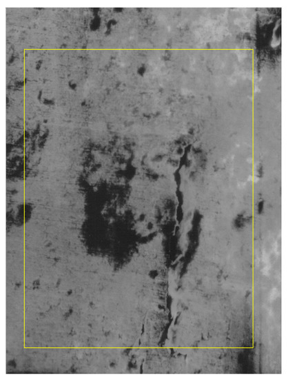
Figure 1.
Original image and a selected area.
Figure 2 shows the attractor reconstruction [20] for the rectangle with yellow sides of the normal area along with a considerable area with microcracks and prominent breakage, conformable to Figure 1. Both attractor reconstructions are presented. In embedding dimension 2 some points were observed, and in embedding dimension 3 some broken lines were noticed. Suitable to Figure 1, we exhibit in Figure 3 the time series (spatial series) produced by the entire area, contained in the yellow frame. Thus, the selected area exhibited every surface morphological modification, due to the presence both of the intact, unaffected areas and of the material zones assailed by fracture.
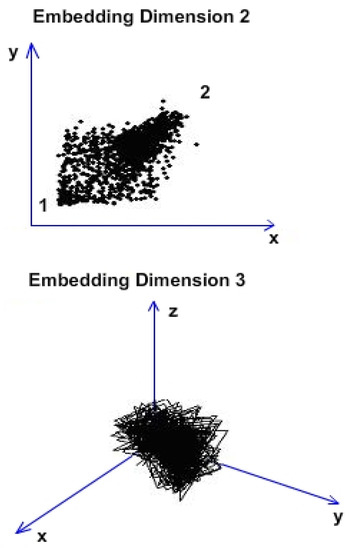
Figure 2.
Attractor reconstruction from Figure 1.

Figure 3.
The time series generated by the selected area.
A slow, slightly steep slope at the time series start, sprinkled with uniform matched values of the entire period, followed by a tendency of mediation in the sawtooth (see solid blue line), is observed in Figure 3. The horizontal green line represents the average value of the series over the entire period considered.
For the second pitch we will investigate the image part that contains the modified area with obvious cracks, selected from the entire available image. Thus, we can say that Figure 4 contains the modified area in total agreement with the WFDM procedure. The choice made was limited to the area with yellow edges and was due to the visual aspect, which was different from the unaffected parts of the material, with the rest remaining in the whole picture.
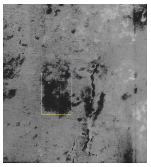
Figure 4.
The selection of the modified area.
Figure 5 shows the attractor reconstruction for the rectangle with yellow sides of the normal area, conformable to Figure 4. Both attractor reconstructions are presented. In embedding dimension 2, some points were observed and in embedding dimension 3 some broken lines were noticed [11]. Suitable to Figure 4, we exhibit in Figure 6 the time series (spatial series) produced by the modified area, a material zone attacked/assailed by fracture. In Figure 6 is presented the time series associated with the selected modified area. A steep slope at the time series beginning with the highest value of entire period, followed by a tendency of mediation in sawtooth (see solid blue line), was observed. The horizontal green line represents the average value of the series over the entire period considered.
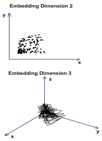
Figure 5.
Attractor reconstruction from Figure 4.

Figure 6.
The time series associated with the selected modified area.
The graphic of the modified area autocorrelation in Figure 7, representing the correlation dimension (CorDim) versus the embedding dimension (EmbDim), shows the slope computation. The (CorDim) versus (EmbDim) slope was 0.2213. The equation of the regression line is y = 0.2213x + 0.4525. R2 (R-Squared or coefficient of determination) was equal to 0.9994, representing that the very good data fit the regression model used.
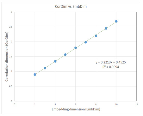
Figure 7.
The slope of the autocorrelation dimension versus the embedding dimension for the modified area.
Figure 8 introduces the original image of the affected/modified area in the yellow border. Figure 9 introduces the binary version of the image in the yellow box. Figure 10 introduces the process of applying the mask to the image, for lacunarity calculation. The blue box represents the area of interest.
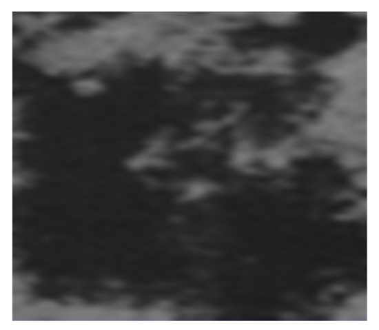
Figure 8.
The original image of the affected/modified area in the yellow border.
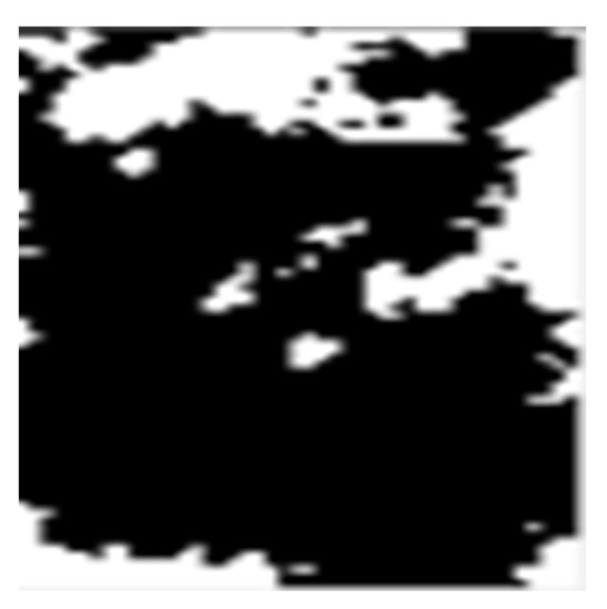
Figure 9.
The binary version of the image in the yellow box.
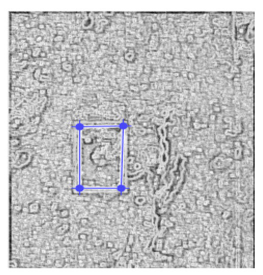
Figure 10.
Applying the mask for lacunarity calculation.
Following the numerical evaluations with the appropriate software of the image to affected/modified area, the values of fractal dimension D = 1.7411, standard deviation , and lacunarity were obtained.
Figure 11 shows the verification of the image in the affected/modified area with the Harmonic and Fractal Image Analyzer Demo software version 5.5.30 [21] of the fractal dimension of the area for various ruler scales r.
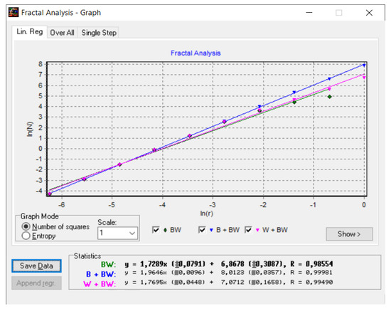
Figure 11.
Graphic of the fractal dimension for the affected/modified area.
Figure 12 represents the three-dimensional graph of the voxel representation of the image in the affected/modified area.
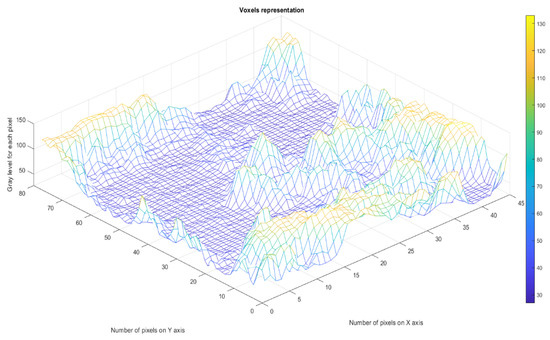
Figure 12.
Voxel representation of the image in the affected/modified area.
The last studied area of the SEM image of Zy-4, in fact the third zone, is the one that refers to the area considered normal—more precisely, the area that remained undeformed and was prepared according to the WFDM protocol. Figure 13, which consists of a sector framed in the yellow rectangle, represents the structure that was considered/remained normal by comparison with the parts affected by microcracks.
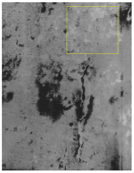
Figure 13.
The selection of a normal area.
Figure 14 shows the attractor reconstruction for the rectangle with yellow sides of the normal area, conformable to Figure 13. Both attractor reconstructions are presented. In embedding dimension 2 some points were observed, and in embedding dimension 3 some broken lines were noticed. Suitable to Figure 13, we exhibit in Figure 15 the time series (spatial series) produced by the normal (unaffected) area, a material zone considered intact.
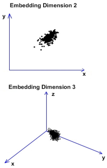
Figure 14.
Attractor reconstruction from Figure 13.

Figure 15.
Time series associated with a normal area.
A steep slope at the time series throughout the entire period accompanied by the tendency to average the peaks and a mediation propensity in sawtooth (see solid blue line) was observed. The horizontal green line represents the average value of the series over the entire period considered.
The graphic of the normal area autocorrelation in Figure 16, representing the correlation dimension (CorDim) versus the embedding dimension (EmbDim), shows the slope computation. The CorDim versus EmbDim slope was 0.1479. The equation of the regression line is y = 0.148x + 0.815. R2 (R-Squared or coefficient of determination) was equal to 0.9842, representing that the very good data fit the regression model used.
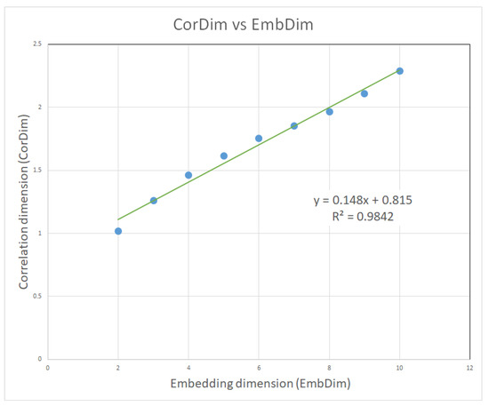
Figure 16.
The slope of the autocorrelation dimension versus the embedding dimension for the normal area.
Figure 17 introduces the original image of the unaffected area in the yellow border. Figure 18 introduces the binary version of the image in the yellow box. Figure 19 introduces the process of applying the mask to the image, for lacunarity calculation. The blue box represents the area of interest.
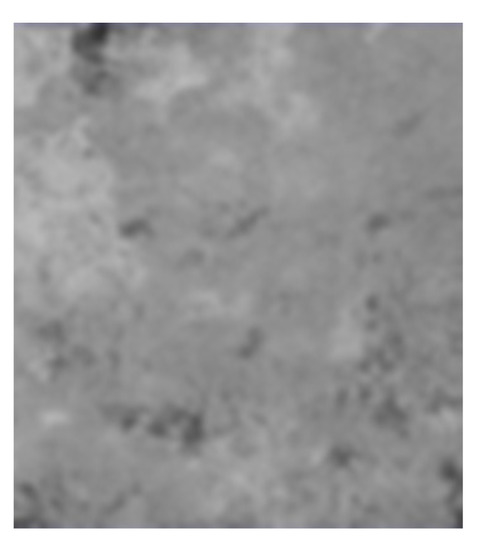
Figure 17.
The original image of the unaffected area in the yellow border.
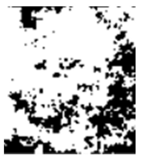
Figure 18.
The binary version of the image in the yellow box.
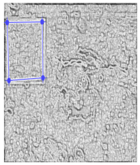
Figure 19.
Applying the mask for lacunarity calculation.
Following the numerical evaluations with the appropriate software of the image to unaffected area, the values of fractal dimension D = 1.8422, standard deviation , and lacunarity were obtained.
Figure 20 represents the three-dimensional graph of the voxel representation for the image in the unaffected area [19,22].
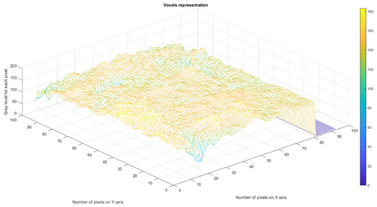
Figure 20.
Voxels representation of the image in the unaffected area.
Figure 21 shows the verification of the image in the unaffected area with the Harmonic and Fractal Image Analyzer Demo software version 5.5.30 of the fractal dimension of the area for various ruler scales r.
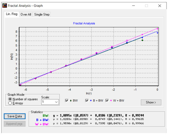
Figure 21.
Graphic of the fractal dimension for the unaffected area.
The carefully conducted research was carried out on 20 SEM images, microfractographs of some samples that presented either the original unmodified area or the modified area. Two distinct areas were selected from each picture, one with a distinct portion that included an area with a normal original structure (unaffected) and another zone with a modified structure affected by microfractures [23].
The conclusive results obtained are presented in the format of a histogram in Figure 22. We thus drew a histogram graphic (a bar data representation) for the correlation dimension function versus the embedding dimension slopes [24,25], with the slopes of the calculated regression lines in the domain between the values/range [0.08, 0.32].
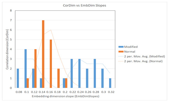
Figure 22.
The histogram of the CorDim vs. EmbDim slopes.
4. Conclusions
This work pursues and completes the complex research initiated in preceding papers, where pictures of the fracture surface of SEM Zy-4 samples are considered by employment of the fractal analysis method and the time-series technique. The fractal analysis method manages to resolve the damage complications and finally to ascertain the morphological parameters of various fractures, documented in SEM images in metal alloys and in Zy-4 SEM pictures. For the Zy-4 SEM picture investigation, we developed a computer software practice that generates a time series (spatial series) associated with the picture, then restores the attractor and calculates its autocorrelation dimension.
Considering the analyzed Figure 1, Figure 4, and Figure 13, we proved that obtaining fractal compositions (organizations) in Zy-4 SEM images (microfractographies) is a reasonable and pragmatic assumption. In addition, the application of fractal analysis to the SEM images of Zy-4 samples and the calculation of fractal dimension and lacunarity was a success of this study.
The fractal numerical valuations of the affected/modified area image of Zy-4 samples were achieved, and the values of fractal dimension D = 1.7411 ± 0.4568 and lacunarity were obtained. In the same conditions, regarding the Zy-4 image for the unaffected area, values of fractal dimension D = 1.8422 ± 0.3278 and lacunarity were achieved.
The results performance, acquired from the topical investigation provided, lead to the conclusions listed below. Thus, the attractors in embedding dimensions 2 and 3 of the entire picture had three connected components, one corresponding to the entire picture, another to the normal (unaffected) area, and the last to the modified (affected) area. The role of these graphic representations is to provide the researcher with notable clues about the anomalies contained in each investigated image.
The CorDim versus EmbDim slope was 0.1479 for the graphic of the normal area autocorrelation and 0.2213 for the modified area autocorrelation. The autocorrelation dimension average for the normal areas was 0.1587, following a normal distribution on the interval [0.11, 0.24] determined on the abscissa. There are no obvious conclusions on the autocorrelation dimension for the modified (affected) areas. As one can see in the histograms diagram, it covered a rather broad interval with two peaks, one between [0.08, 0.18] and the other between [0.19, 0.32], with both intervals being determined on the abscissa. The correlation dimension function versus the embedding dimension slopes had slopes of the calculated regression lines in the domain between the values/range [0.08, 0.32].
Author Contributions
Conceptualization, V.-P.P. and M.-A.P.; methodology, V.-P.P.; software, V.-A.P.; validation, V.-P.P., M.-A.P. and V.-A.P.; formal analysis, V.-P.P., M.-A.P. and V.-A.P.; investigation, V.-A.P. and M.-A.P.; resources, V.-A.P. and M.-A.P.; data curation, V.-A.P.; writing—original draft preparation, V.-P.P.; writing—review and editing, M.-A.P. and V.-P.P.; visualization, V.-A.P.; supervision, V.-P.P.; project administration, V.-P.P. All authors have read and agreed to the published version of the manuscript.
Funding
This research received no external funding.
Institutional Review Board Statement
Not applicable.
Informed Consent Statement
Not applicable.
Data Availability Statement
The data used to support the findings of this study cannot be accessed due to commercial confidentiality.
Acknowledgments
The co-authors M.-A.P., V.-A.P. and V.-P.P. would like to thank Jenica Paun, for her continuous kind support.
Conflicts of Interest
The authors declare no conflict of interest.
References
- Moan, G.D.; Rudling, P. Zirconium in the Nuclear Industry, 13th International Symposium; ASTM-STP 1423; American Society for Testing & Materials: West Conshohocken, PA, USA, 2002; pp. 673–701. [Google Scholar]
- Kaddour, D.; Frechinet, S.; Gourgues, A.F.; Brachet, J.C.; Portier, L.; Pineau, A. Experimental determination of creep properties of Zirconium alloys together with phase transformation. Scr. Mater. 2004, 51, 515–519. [Google Scholar] [CrossRef]
- Brenner, R.; Béchade, J.L.; Bacroix, B. Thermal creep of Zr–Nb1%–O alloys: Experimental analysis and micromechanical modelling. J. Nucl. Mater. 2002, 305, 175–186. [Google Scholar] [CrossRef]
- Olteanu, M.; Paun, V.P.; Tanase, M. Fractal analysis of zircaloy-4 fracture surface, Conference on Equipments, Installations and Process Engineering. Rev. Chim. 2005, 56, 97–100. [Google Scholar]
- Takens, F. Detecting strange attractors in turbulence. Lect. Notes Math. 1981, 898, 366–381. [Google Scholar]
- Takens, F. On the Numerical Determination of the Dimension of an Attractor. In Dynamical Systems and Bifurcations; Braaksma, B.L.J., Broer, H.W., Takens, F., Eds.; Springer: Berlin/Heidelberg, Germany, 1985; pp. 99–106. [Google Scholar]
- Xu, L.; Shi, Y. Notes on the Global Attractors for Semigroup. Int. J. Mod. Nonlinear Theory Appl. 2013, 2, 219–222. [Google Scholar] [CrossRef][Green Version]
- Sauer, T.; Yorke, J.; Casdagli, M. Embedology. J. Stat. Phys. 1991, 65, 579–616. [Google Scholar] [CrossRef]
- Mandelbrot, B.B.; Passoja, D.E.; Paullay, A.J. Fractal character of fracture surfaces of metals. Nature 1984, 308, 721–722. [Google Scholar] [CrossRef]
- Mandelbrot, B. Fractal Geometry of Nature; Freeman: New York, NY, USA, 1983; pp. 25–57. [Google Scholar]
- Passoja, D.E.; Psioda, J.A. Fractography in Materials Science; ASTM STP: American Society for Testing & Materials: West Conshohocken, PA, USA, 1981; pp. 335–386. [Google Scholar]
- Mattfeldt, T. Nonlinear deterministic analysis of tissue texture: A stereological study on mastopathic and mammary cancer tissue using chaos theory. J. Microsc. 1997, 185, 47–66. [Google Scholar] [CrossRef] [PubMed]
- Peitgen, H.-O.; Jurgens, H.; Saupe, D. Chaos and Fractals. In New Frontiers of Science; Springer: Berlin/Heidelberg, Germany, 1992. [Google Scholar]
- Thompson, J.M.T.; Stewart, H.B. Nonlinear Dynamics and Chaos; John Wiley and Sons: Hoboken, NJ, USA, 1986. [Google Scholar]
- Available online: https://www.mathworks.com/matlabcentral/answers/how-to-estimate-correlation-integrals-and-local-slopes-for-embedding-dimension (accessed on 7 March 2022).
- Datseris, G.; Kottlarz, I.; Braun, A.P.; Parlitz, U. Estimating the fractal dimension: A comparative review and open source implementations. arXiv 2021, arXiv:2109.05937v1. [Google Scholar]
- Falconer, K. Fractal Geometry: Mathematical Foundations and Applications, 3rd ed.; John Wiley & Sons, Ltd.: Chichester, UK, 2014. [Google Scholar]
- Paun, V.P. Fractal surface analysis of Zircaloy-4 SEM micrographs using the time-series method. Cent. Eur. J. Phys. 2009, 7, 264–269. [Google Scholar] [CrossRef]
- Nichita, M.V.; Paun, M.A.; Paun, V.A.; Paun, V.P. Fractal Analysis of Brain Glial Cells. Fractal Dimension and Lacunarity. Univ. Politeh. Buchar. Sci. Bull. Ser. A Appl. Math. Phys. 2019, 81, 273–284. [Google Scholar]
- Bordescu, D.; Paun, M.A.; Paun, V.A.; Paun, V.P. Fractal Analysis of Neuroimagistics. Lacunarity Degree, a Precious Indicator in the Detection of Alzheimer’s Disease. Univ. Politeh. Buchar. Sci. Bull. Ser. A Appl. Math. Phys. 2018, 80, 309–320. [Google Scholar]
- Available online: https://astronomy.swin.edu.au/~pbourke/fractals/fracdim/index.html (accessed on 3 September 2021).
- Nichita, M.V.; Paun, M.A.; Paun, V.A.; Paun, V.P. Image Clustering Algorithms to Identify Complicated Cerebral Diseases. Description and Comparaisons. IEEE Access 2020, 8, 88434–88442. [Google Scholar] [CrossRef]
- Rempe, M.; Mitchell, T.M.; Renner, J.; Smith, S.A.F.; Bistacchi, A.; Di Toro, G. The relationship between microfracture damage and the physical properties of fault-related rocks: TheGole Larghe Fault Zone, Italian SouthernAlps. J. Geophys. Res. Solid Earth 2018, 123, 7661–7687. [Google Scholar] [CrossRef]
- Scott, D.W. Statistics: A Concise Mathematical Introduction for Students, Scientists, and Engineers; John Wiley & Sons, Inc.: Hoboken, NJ, USA, 2020. [Google Scholar]
- Michalak, K.P. Estimating correlation dimension of high-dimensional signals—Quick algorithm. AIP Adv. 2018, 8, 105201. [Google Scholar] [CrossRef]
Publisher’s Note: MDPI stays neutral with regard to jurisdictional claims in published maps and institutional affiliations. |
© 2022 by the authors. Licensee MDPI, Basel, Switzerland. This article is an open access article distributed under the terms and conditions of the Creative Commons Attribution (CC BY) license (https://creativecommons.org/licenses/by/4.0/).