Asymptotic Synchronization of Fractional-Order Complex Dynamical Networks with Different Structures and Parameter Uncertainties

Abstract

This paper deals with the asymptotic synchronization of fractional-order complex dynamical networks with different structures and parameter uncertainties (FCDNDP). Firstly, the FCDNDP model is proposed by the Riemann–Liouville (R-L) fractional derivative. According to the property of fractional calculus and the Lyapunov direct method, an original controller is proposed to achieve the asymptotic synchronization of FCDNDP. Our controller is more adaptable and effective than those in other literature. Secondly, a sufficient condition is given for the asymptotic synchronization of FCDNDP based on the asymptotic stability theorem and the matrix inequality technique. Finally, the numerical simulations verify the effectiveness of the proposed method.

1. Introduction

Fractional calculus is a popularization of integrals and differentials of integer orders. Although the history of fractional calculus and integer calculus is not very discrepant, the results show that fractional calculus is very important for the expression of the model. In addition to the memory function of fractional calculus, the characterization of a complex system has the advantages of simple modeling, clear physical meaning of parameters and exact description [1,2,3]. Because of these advantages, it can be applied in many fields, such as physics [4], engineering [2], chemistry [5], information processing [6], secure communication [7], thermal systems [8], and robot control problems [9], etc. Since fractional-order calculus makes a tool more precise with regard to the description of memory and genetic properties of multifarious materials and processes, it is extremely important to introduce fractional calculus into complex dynamic network models.

Complex networks have been widely used in different disciplines such as physics, biology and sociology because of complex network topology and spatiotemporal evolution of systems [10]. In real life, they might be applied in neural networks [11], social networks [12], ecological networks [13], electric networks [14] and other networks. These networks share or exchange opinions with each other in a certain link based on multi-nodes, so that the complex network can be used in nature, as well as various systems in society. This has made many scholars study complex networks.

Since chaotic synchronization is proposed, the synchronization of complex networks has become a popular topic in the field of complex networks. Because the fractional-order complex network with synchronous behavior is a common and vital nonlinear phenomenon, it exists widely in nature and human society. Therefore, understanding and controlling the fractional-order synchronization of complex networks has theoretical and practical significance. In addition, the controllability of fractional complex networks has turned into a popular topic, and our ability to control natural or technological systems is reflected in our understanding and ultimate proof of them [15]. Hence, the study the synchronization problem of fractional complex networks has important implications. So far, many synchronization methods are used to research complex networks, such as global synchronization [16], adaptive synchronization [17], projection synchronization [18] and finite time synchronization [19].

However, most papers study the synchronization problem of fractional-order systems with the same structure. In practical application, due to the inevitable mismatch of parameters and functions in genuine execution, the drive system and the response system are not quite the same [20]. From an engineering viewpoint, it is truly challenging to keep the two systems consistent. Therefore, it is of extraordinary importance to research the synchronization of complex networks with different structures.

The uncertainty of parameters should be considered due to the existence of environmental disturbances when we analyze the stability of complex networks. We know that the modified model parameters are usually unable to get an accurate value. The main reason is that when the model is applied to actual engineering, it will be affected by interference from the environment, leading to the uncertainty of parameters. In the dynamic behavior analysis of a nonlinear system, the influence of such parameter uncertainties cannot be ignored, because they may damage the stability, synchronization or other characteristics of the system [21]. Thus, it is indispensable to study the system problems with uncertain parameters.

Although the system with parameter uncertainty will make the system more complex, the complex network with parameter uncertainty is closer to reality. Therefore, it has become a hot area of research for scholars. In 2008, based on the linear matrix inequalities (LMI) technique, Shen gave a sufficient condition for the boundedness ensure of neural networks with uncertain parameters [22]. In 2012, Wong derived the robust synchronization of fractional-order complex networks with uncertain parameters based on the nature of a Kronecker product and the stability of fractional-order systems by applying nonlinear control [23]. In 2013, Li designed a state estimator for the problem of fractal-order complex networks with uncertain parameters by using LMI technology and matrix singular value decomposition [24]. In 2015, combining the Lyapunov stability theorem and homeomorphic mapping theorem, Samli obtained some prime sufficient conditions for the existence uniqueness and asymptotic stability [25]. In 2016, based on the fractional Lyapunov direct method, Ding obtained a new standard for global projection synchronization of the nonuniform fractional neural networks [26]. In 2018, using the property of fractional calculus and the Lyapunov direct method, Hu revealed some new properties of fractional calculus and asymptotic stability theorems for nonautonomous fractional calculus systems with Riemann–Liouville derivatives [27]. In 2020, Udpin derived a new exponential stability standard for uncertain discrete-time neural networks based on the discrete Halanay inequality and some other inequalities techniques [28]. In 2022, based on the property of fractional calculus and the fractional direct Lyapunov method, Aadhithiyan obtained a method to realize the asymptotic synchronization of the drive and response systems in nonidentical complex networks using neoteric control [29]. Because the system contains the parameter uncertainty, the interference of the system is very large still, so how to reduce or eliminate the influence of the uncertainty is an imminent issue. Coupled with the need for synchronization of nonidentical complex networks in the industry, the study of synchronization of fractional-order complex networks with different structures is still necessary.

The primary contribution of this paper can be briefly summed up as follows: (i) we propose a new fractal-order complex dynamical network model with different structures and parameter uncertainties; (ii) we conduct synchronization analysis of FCDNDP. Based on fractional differential theory and the Lyapunov direct method, we establish the criterion to guarantee the synchronization of the drive response model; (iii) contrasted with the existing results in the literature, the method is more general and less conservative.

2. Preliminaries

Definition 1

([1]). The Caputo derivative with ξ-order of function is defined as

$$\begin{array}{c}\hfill {}_{t_0}^C{D}_t^{\xi }f\left(t\right)=\frac{1}{\Gamma (m-\xi )}{\int }_{t_0}^t{(t-\upsilon )}^{m-\xi -1}{f}^{\left(m\right)}\left(\upsilon \right)d\upsilon ,\end{array}$$

(1)

where $\Gamma (·)$ is Gamma function, $t\ge 0,m-1<\xi <m,m\in {\mathbb{Z}}^{+}$. Particularly, when $0<\xi <1,$

$$\begin{array}{c}\hfill {}_{t_0}^C{D}_t^{\xi }f\left(t\right)=\frac{1}{\Gamma (1-\xi )}{\int }_{t_0}^t{(t-\upsilon )}^{-\xi }{f}^{\left(m\right)}\left(\upsilon \right)d\upsilon .\end{array}$$

(2)

Definition 2

([1]). The Riemann–Liouville derivative with ξ-order of function is defined as

$$\begin{array}{c}\hfill {}_{t_0}^R{D}_t^{\xi }f\left(t\right)=\frac{1}{\Gamma \left(\xi \right)}{\int }_{t_0}^t\frac{f\left(\upsilon \right)}{{(t-\upsilon )}^{1-\xi }}d\upsilon ,\end{array}$$

(3)

where $\Gamma (·)$ is Gamma function, and $0<\xi <1$.

Lemma 1

([30]). When $f\left(t\right)$ has a continuous first derivative, then

$$\begin{array}{c}\hfill {}_{t_0}^C{D}_t^{\xi }({\displaystyle \frac{1}{2}}{f}^T\left(t\right)Qf\left(t\right))\le f^{T}Q{}_{t_0}^C{D}_t^{\xi }f\left(t\right),\end{array}$$

(4)

where $\xi \in (0,1)$ and Q is an arbitrary n-order positive definite matrix.

Lemma 2

([31]). Let $\epsilon >0$, for ∀ $W\in {\mathbb{R}}^n$, $H\in {\mathbb{R}}^n$ and the $n\times n$ matrix A, then the following formula holds

$$\begin{array}{c}\hfill 2W^{T}AH\le {\epsilon }^{-1}{W}^{T}A{A}^{T}W+\epsilon H^{T}H.\end{array}$$

(5)

Property 1

([1]). When $0<\xi <1$ and $f\left(t\right)$ is a continuous function, we have

$${}_{t_0}^R{D}_t^{-\xi }{}_{t_0}^C{D}_t^{\xi }f\left(t\right)=f\left(t\right)-f\left(t_0\right).$$

Property 2

([1]). Let C be the constant; we can obtain

$${}_{t_o}^R{D}_t^{-\xi }C=\frac{C{\left(t-t_o\right)}^{-\xi }}{\Gamma (1-\xi )},$$

where $0<\xi <1$ and $\Gamma (·)$ is Gamma function.

Lemma 3

([27]). Let $f\left(t\right)$ be a continuous function, then the following formula holds

$${}_{t_0}^R{D}_t^{\xi }\left(f\left(t\right)-f\left(t_0\right)\right)={}_{t_0}^C{D}_t^{\xi }f\left(t\right),$$

where $0<\xi <1$.

Lemma 4

([27]). If $\xi \in (0,1)$, $f\left(t\right)$ is the continuously differentiable function, then

$$\begin{array}{c}\hfill {}_{t_0}^R{D}_t^{\xi }{f}^T\left(t\right)Pf\left(t\right)\le \frac{{(t-t_0)}^{-\xi }}{\Gamma (1-\xi )}{f}^T\left(t_0\right)Pf\left(t_0\right)+2f^T\left(t\right)P_{t_0}^R{D}_t^{\xi }(f\left(t\right)-f\left(t_0\right)),\end{array}$$

(6)

where $P\in {\mathbb{R}}^{n\times n}$ is a positive definite matrix.

Lemma 5

([27]). Let $y=0$ be an equilibrium point of the nonautonomous fractional differential equation ${}_{t_0}^R{D}_t^{\xi }y\left(t\right)=g(t,y)$ which satisfies the Lipschitz constant $c>0$, and $\xi \in (0,1)$. If we suppose that there is a Lyapunov function $v\left(t\right)=V(t,y)$ and some class-K functions ${\lambda }_p(p=1,2,3)$, which satisfy the following equations

$$\begin{array}{c}\hfill {\lambda }_1(\parallel y\parallel )\le v\left(t\right)\le {\lambda }_2(\parallel y\parallel ),\end{array}$$

(7)

$$\begin{array}{c}\hfill {}_{t_o}^R{D}_t^{\xi }v\le \frac{{\left(t-t_o\right)}^{-\xi }}{\Gamma (1-\xi )}v\left(t_o\right)-{\lambda }_3\left(y\left(t\right)\right),\end{array}$$

(8)

where for all $t\ge t_0$, then the equilibrium point of the fractional-order equation is asymptotically stable.

Model Description

In this paper, we can consider the following drive system and response system of fractional-order complex dynamical networks, as follows [29]:

$$\begin{array}{c}\hfill {}_{t_0}^C{D}_t^{\xi }{\varphi }_p\left(t\right)=A{\varphi }_p\left(t\right)+B\gamma {\varphi }_p\left(t\right)+c\sum _{q=1}^N{d}_{pq}{\Lambda }_1{\varphi }_q\left(t\right),\end{array}$$

(9)

and

$$\begin{array}{c}\hfill {}_{t_0}^C{D}_t^{\xi }{\phi }_p\left(t\right)=(E_0+\Delta E){\phi }_p\left(t\right)+(G_0+\Delta G)\eta {\phi }_p\left(t\right)+k\sum _{q=1}^N{L}_{pq}{\Lambda }_2{\phi }_q\left(t\right)+{\omega }_p\left(t\right),\end{array}$$

(10)

where $0<\xi <1$, ${\varphi }_p\left(t\right)$ and ${\phi }_p\left(t\right)$ are the state of the p -node of the above systems, A and $E_0$ are the real constant matrices, and B and $G_0$ indicate the weight association matrices. $\gamma {\varphi }_p\left(t\right)$ and $\eta {\phi }_p\left(t\right)$ express the vector-valued nonlinear functions. D = ${\left(d_{pq}\right)}_{N\times N}$ and L = ${\left(l_{pq}\right)}_{N\times N}$ are the external coupling matrices which denote the link between node p and q. If they have a direct link between node p to q, $d_{pq}>0$ and $l_{pq}>0$; otherwise, $d_{pq}=0$ and $l_{pq}=0$. $\Lambda$ refers to the internal coupling matrix, a link between two subsystems. ${\omega }_p\left(t\right)$ expresses the control input. $\Delta E$ and $\Delta G$ are the parameter uncertainties, such that,

$$\begin{array}{c}\hfill E=(E_0+\Delta E),G=(G_0+\Delta G).\end{array}$$

(11)

The parameter uncertainties $\Delta E$ and $\Delta G$ can be given by

$$\begin{array}{c}\hfill E_0\left(t\right)=H_1{\Xi }_1{K}_1,G_0\left(t\right)=H_2{\Xi }_2{K}_2,\end{array}$$

(12)

where $H_i$ and $K_i(i=1,2)$ are positive constant matrices, and uncertain ${\Xi }_i\left(t\right)(i=1,2)$ are the matrices which are unknown and satisfy the following condition

$$\begin{array}{c}\hfill {\Xi }_i\left(t\right){\left({\Xi }_i\left(t\right)\right)}^T\le I,\end{array}$$

(13)

where I is an identity matrix.

We consider that the drive system is not quite the same as the response system; then, the error vector is defined by

$$\begin{array}{c}\hfill {\upsilon }_p\left(t\right)={\phi }_p\left(t\right)-{\varphi }_p\left(t\right).\end{array}$$

(14)

The error system can be expressed by

$$\begin{array}{c}\hfill {}_{t_0}^C{D}_t^{\xi }{\upsilon }_p\left(t\right)={}_{t_0}^C{D}_t^{\xi }{\phi }_p\left(t\right){-}_{t_0}^C{D}_t^{\xi }{\varphi }_p\left(t\right).\end{array}$$

(15)

By substituting (9) and (10) into (15), we can write

$$\begin{array}{c}\hfill \begin{array}{cc}\hfill {}_{t_0}^C{D}_t^{\xi }{\upsilon }_p\left(t\right)=& (E_0+\Delta E){\phi }_p\left(t\right)+(G_0+\Delta G)\eta {\phi }_p\left(t\right)+k\sum _{q=1}^N{L}_{pq}{\Lambda }_2{\phi }_q\left(t\right)\hfill \\ & -A{\varphi }_p\left(t\right)-B\gamma {\varphi }_p\left(t\right)-c\sum _{q=1}^N{d}_{pq}{\Lambda }_1{\varphi }_q\left(t\right).\hfill \end{array}\end{array}$$

(16)

One can obtain

$$\begin{array}{cc}\hfill {}_{t_0}^C{D}_t^{\xi }{\upsilon }_p\left(t\right)=& (E_0+\Delta E){\phi }_p\left(t\right)-A{\varphi }_p\left(t\right)-(E_0+\Delta E){\varphi }_p\left(t\right)+(E_0+\Delta E){\varphi }_p\left(t\right)\hfill \\ & +(G_0+\Delta G)\eta {\phi }_p\left(t\right)-B\gamma {\varphi }_p\left(t\right)-(G_0+\Delta G)\eta {\varphi }_p\left(t\right)\hfill \\ & +(G_0+\Delta G)\eta {\varphi }_p\left(t\right)+k\sum _{q=1}^N{L}_{pq}{\Lambda }_2{\phi }_q\left(t\right)-c\sum _{q=1}^N{d}_{pq}{\Lambda }_1{\varphi }_q\left(t\right)\hfill \\ & -k\sum _{q=1}^N{L}_{pq}{\Lambda }_2{\varphi }_q\left(t\right)+k\sum _{q=1}^N{L}_{pq}{\Lambda }_2{\varphi }_q\left(t\right)+{\omega }_p\left(t\right).\hfill \end{array}$$

(17)

Assumption A1.

For any $p=1,2,···,N$, the nonlinear function $f_p(·)$ satisfies the Lipschitz condition if ∃ a constant $c>0$, such that

$$\begin{array}{c}\hfill |f_p\left({\chi }_1\right)-f_p\left({\chi }_2\right)|\le c|{\chi }_1-{\chi }_2|,{\chi }_1,{\chi }_2\in \mathbb{R}.\end{array}$$

(18)

3. Main Results

In this section, studying the asymptotic synchronization problem of FCDNDP is similar to the stability analysis of the equilibrium point error model. By applying the $R-L$ fractional derivative, we initially propose an original controller and then present the vital criteria for asymptotic stability.

Theorem 1.

Let the Assumption 1 hold and scalar $0<\xi <1$; the FCDNDP is asymptotically stable if the controller of form (ii) satisfies the criteria (i):

(i) $\Omega <0,$

(ii) ${\omega }_p\left(t\right)=(A-E){\varphi }_p\left(t\right)+B\gamma {\phi }_p\left(t\right)-G\eta {\phi }_p\left(t\right)+c{\displaystyle \sum _{q=1}^N}{d}_{pq}{\Lambda }_1{\phi }_q\left(t\right)-k{\displaystyle \sum _{q=1}^N}{L}_{pq}{\Lambda }_2{\varphi }_q\left(t\right),$where

$$\begin{array}{cc}\hfill \Omega =& P{E}_0+E_0^T\left(t\right)P+{ϵ}_1^{-1}P{H}_1{H}_1^{T}P+{ϵ}_1{T}_1{T}_1^T+{ϵ}_2^{-1}P{H}_2{H}_2^{T}P+{ϵ}_2{T}_2{T}_2^T+{ϵ}_3{\theta }_1\hfill \\ & +{ϵ}_3^{-1}PG{G}^{T}P+{ϵ}_4^{-1}PB{B}^{T}X+{ϵ}_4{\theta }_2+k\sum _{q=1}^N{L}_{pq}{\Lambda }_2+c\sum _{q=1}^N{d}_{pq}{\Lambda }_1.\hfill \end{array}$$

Proof. 

It follows from the error system (17) that the Lyapunov function can be designed as

$$\begin{array}{c}\hfill V\left(t\right)={\upsilon }_p^T\left(t\right)P{\upsilon }_p\left(t\right).\end{array}$$

(19)

Computing the derivative of the (19) along the error system, we can obtain

$$\begin{array}{c}\hfill {}_{t_0}^R{D}_t^{\xi }{V}_p\left(t\right)={}_{t_0}^R{D}_t^{\xi }\left({\upsilon }_p^T\left(t\right)P{\upsilon }_p\left(t\right)\right).\end{array}$$

(20)

According to Lemma 4, (20) can be composed as

$$\begin{array}{c}\hfill {}_{t_0}^R{D}_t^{\xi }{V}_p\left(t\right)=\frac{{(t-t_0)}^{-\xi }}{\Gamma (1-\xi )}\left({\upsilon }_p^T\left(t_0\right)P{\upsilon }_p\left(t_0\right)\right)+2{\upsilon }_p^T\left(t\right)P_{t_0}^R{D}_t^{\xi }({\upsilon }_p\left(t\right)-{\upsilon }_p\left(t_0\right)).\end{array}$$

(21)

Based on the Lemma 3, (21) can be composed as

$$\begin{array}{c}\hfill {}_{t_0}^R{D}_t^{\xi }{V}_p\left(t\right)=\frac{{(t-t_0)}^{-\xi }}{\Gamma (1-\xi )}\left({\upsilon }_p^T\left(t_0\right)P{\upsilon }_p\left(t_0\right)\right)+2{\upsilon }_p^T\left(t\right)P_{t_0}^C{D}_t^{\xi }{\upsilon }_p\left(t\right).\end{array}$$

(22)

Substituting the error system (17) into the (22), we can obtain

$$\begin{array}{cc}\hfill {}_{t_0}^R{D}_t^{\xi }{V}_p\left(t\right)=& \frac{{(t-t_0)}^{-\xi }}{\Gamma (1-\xi )}\left({\upsilon }_p^T\left(t_0\right)P{\upsilon }_p\left(t_0\right)\right)+2{\upsilon }_p^T\left(t\right)P\{(E_0+\Delta E){\phi }_p\left(t\right)-A{\varphi }_p\left(t\right)\hfill \\ & -(E_0+\Delta E){\varphi }_p\left(t\right)+(E_0+\Delta E){\varphi }_p\left(t\right)+(G_0+\Delta G)\eta {\phi }_p\left(t\right)-B\gamma {\varphi }_p\left(t\right)\hfill \\ & -(G_0+\Delta G)\eta {\varphi }_p\left(t\right)+(G_0+\Delta G)\eta {\varphi }_p\left(t\right)+k\sum _{q=1}^N{L}_{pq}{\Lambda }_2{\phi }_q\left(t\right)\hfill \\ & -c\sum _{q=1}^N{d}_{pq}{\Lambda }_1{\varphi }_q\left(t\right)-k\sum _{q=1}^N{L}_{pq}{\Lambda }_2{\varphi }_q\left(t\right)+k\sum _{q=1}^N{L}_{pq}{\Lambda }_2{\varphi }_q\left(t\right)+{\omega }_p\left(t\right)\}.\hfill \end{array}$$

(23)

Applying the controller ${\omega }_p\left(t\right)$ into (23), we have the following formula

$$\begin{array}{cc}\hfill {}_{t_0}^R{D}_t^{\xi }{V}_p\left(t\right)=& \frac{{(t-t_0)}^{-\xi }}{\Gamma (1-\xi )}\left({\upsilon }_p^T\left(t_0\right)P{\upsilon }_p\left(t_0\right)\right)+2{\upsilon }_p^T\left(t\right)P\{(E_0+\Delta E){\phi }_p\left(t\right)-A{\varphi }_p\left(t\right)\hfill \\ & -(E_0+\Delta E){\varphi }_p\left(t\right)+(E_0+\Delta E){\varphi }_p\left(t\right)+(G_0+\Delta G)\eta {\phi }_p\left(t\right)\hfill \\ & -B\gamma {\varphi }_p\left(t\right)-(G_0+\Delta G)\eta {\varphi }_p\left(t\right)+(G_0+\Delta G)\eta {\varphi }_p\left(t\right)\hfill \\ & +k\sum _{q=1}^N{L}_{pq}{\Lambda }_2{\phi }_q\left(t\right)-c\sum _{q=1}^N{d}_{pq}{\Lambda }_1{\varphi }_q\left(t\right)+B\gamma {\phi }_p\left(t\right)\hfill \\ & -k\sum _{q=1}^N{L}_{pq}{\Lambda }_2{\varphi }_q\left(t\right)+k\sum _{q=1}^N{L}_{pq}{\Lambda }_2{\varphi }_q\left(t\right)+(A-E){\varphi }_p\left(t\right)\hfill \\ & -G\eta {\phi }_p\left(t\right)+c\sum _{q=1}^N{d}_{pq}{\Lambda }_1{\phi }_q\left(t\right)-k\sum _{q=1}^N{L}_{pq}{\Lambda }_2{\varphi }_q\left(t\right)\}.\hfill \end{array}$$

(24)

The above formula can be simplified as

$$\begin{array}{cc}\hfill {}_{t_0}^R{D}_t^{\xi }{V}_p\left(t\right)=& \frac{{(t-t_0)}^{-\xi }}{\Gamma (1-\xi )}\left({\upsilon }_p^T\left(t_0\right)P{\upsilon }_p\left(t_0\right)\right)+2{\upsilon }_p^T\left(t\right)P\{(E_0+\Delta E){\upsilon }_p\left(t\right)\hfill \\ & +(G_0+\Delta G)\eta {\upsilon }_p\left(t\right)+k\sum _{q=1}^N{L}_{pq}{\Lambda }_2{\upsilon }_q\left(t\right)\hfill \\ & +B\gamma {\upsilon }_p\left(t\right)+c\sum _{q=1}^N{d}_{pq}{\Lambda }_1{\upsilon }_q\left(t\right)\}.\hfill \end{array}$$

(25)

Utilizing the Lemma 2 into (25), we have

$$\begin{array}{cc}\hfill 2{\upsilon }_p^T\left(t\right)P(E_0+\Delta E){\upsilon }_p\left(t\right)\le & 2{\upsilon }_p^T\left(t\right)P{E}_0{\upsilon }_p\left(t\right)+2{\upsilon }_p^T\left(t\right)P\Delta E{\upsilon }_p\left(t\right)\hfill \\ \hfill \le & {\upsilon }_p^T\left(t\right)(P{E}_0+E_0^{T}P){\upsilon }_p\left(t\right)+2{\upsilon }_p^T\left(t\right)P{H}_1{\Xi }_1{T}_1{\upsilon }_p\left(t\right)\hfill \\ \hfill \le & {\upsilon }_p^T\left(t\right)(P{E}_0+E_0^{T}P){\upsilon }_p\left(t\right)+{\upsilon }_p^T\left(t\right){ϵ}_1^{-1}P{H}_1{H}_1^{T}X{\upsilon }_p\left(t\right)\hfill \\ & +{\upsilon }_p^T\left(t\right){ϵ}_1{T}_1{T}_1^T{\upsilon }_p\left(t\right)\hfill \\ \hfill \le & {\upsilon }_p^T\left(t\right)\{P{E}_0+E_0^T\left(t\right)P+{ϵ}_1^{-1}P{H}_1{H}_1^{T}P+{ϵ}_1{T}_1{T}_1^T\}{\upsilon }_p\left(t\right),\hfill \end{array}$$

(26)

and

$$\begin{array}{cc}\hfill 2{\upsilon }_p^T\left(t\right)P(G_0+\Delta G)\eta {\upsilon }_p\left(t\right)& \le {\upsilon }_p^T\left(t\right)\{{ϵ}_2^{-1}P{H}_2{H}_2^{T}P+{ϵ}_2{T}_2{T}_2^T+{ϵ}_3^{-1}PG{G}^{T}P+{ϵ}_3{\theta }_1\}\hfill \\ \hfill 2{\upsilon }_p^T\left(t\right)PB\gamma {\upsilon }_p\left(t\right)& \le {\upsilon }_p^T\left(t\right)\{{ϵ}_4^{-1}PB{B}^{T}P+{ϵ}_4{\theta }_2\}.\hfill \end{array}$$

(27)

By substituting (26) and (27) into (25), we get

$$\begin{array}{cc}\hfill {}_{t_0}^R{D}_t^{\xi }{V}_p\left(t\right)\le & \frac{{(t-t_0)}^{-\xi }}{\Gamma (1-\xi )}\left({\upsilon }_p^T\left(t_0\right)P{\upsilon }_p\left(t_0\right)\right)+2{\upsilon }_p^T\left(t\right)\{P{E}_0+E_0^T\left(t\right)P\hfill \\ \hfill & +{ϵ}_1^{-1}P{H}_1{H}_1^{T}P+{ϵ}_1{T}_1{T}_1^T+{ϵ}_2^{-1}P{H}_2{H}_2^{T}P\hfill \\ \hfill & +{ϵ}_2{T}_2{T}_2^T+{ϵ}_3^{-1}PG{G}^{T}P+{ϵ}_3{\theta }_1+{ϵ}_4^{-1}PB{B}^{T}P+{ϵ}_4{\theta }_2\hfill \\ \hfill & +k\sum _{q=1}^N{L}_{pq}{\Lambda }_2+c\sum _{q=1}^N{d}_{pq}{\Lambda }_1\}{\upsilon }_p\left(t\right).\hfill \end{array}$$

(28)

The above formula can be further simplified as

$$\begin{array}{cc}\hfill {}_{t_0}^R{D}_t^{\xi }{V}_p\left(t\right)& \le \frac{{(t-t_0)}^{-\xi }}{\Gamma (1-\xi )}\left({\upsilon }_p^T\left(t_0\right)P{\upsilon }_p\left(t_0\right)\right)-{\lambda }_{min}(-\Omega ){\upsilon }_p{\left(t\right)}^T{\upsilon }_p\left(t\right)\hfill \\ \hfill & \le \frac{{(t-t_0)}^{-\xi }}{\Gamma (1-\xi )}\left({\upsilon }_p^T\left(t_0\right)P{\upsilon }_p\left(t_0\right)\right)-\frac{{\lambda }_{min}(-\Omega )}{{\lambda }_{max}\left(P\right)}{\upsilon }_p{\left(t\right)}^{T}P{\upsilon }_p\left(t\right)\hfill \\ \hfill & \le \frac{{(t-t_0)}^{-\xi }}{\Gamma (1-\xi )}\left({\upsilon }_p^T\left(t_0\right)P{\upsilon }_p\left(t_0\right)\right)-\chi V_p\left(t\right),\hfill \end{array}$$

(29)

where $\chi =\frac{{\lambda }_{min}(-\Omega )}{{\lambda }_{max}\left(P\right)}$, utilizing Lemma 5, and if $\Omega <0$ is satisfied, we infer that the error system (17) is asymptotically stable. Then, we find that the FCDNDP is asymptotically synchronized under the original feedback controller. □

In the light of the above Theorem 1, we can obtain the following corollary.

Corollary 1.

If the fractional-order complex network is composed of N nodes, which can be depicted as

$$\begin{array}{c}\hfill {}_{t_0}^C{D}_t^{\xi }{\varphi }_p\left(t\right)=A{\varphi }_p\left(t\right)+Q{\varphi }_p\left(t\right)+B\gamma {\varphi }_p\left(t\right)+c\sum _{q=1}^N{d}_{pq}{\Lambda }_1{\varphi }_q\left(t\right),\end{array}$$

(30)

and

$$\begin{array}{c}\hfill {}_{t_0}^C{D}_t^{\xi }{\phi }_p\left(t\right)=E{\phi }_p\left(t\right)+Y{\phi }_p\left(t\right)+G\eta {\phi }_p\left(t\right)+k\sum _{q=1}^N{L}_{pq}{\Lambda }_2{\phi }_q\left(t\right)+{\omega }_p\left(t\right),\end{array}$$

(31)

which is similar to system (9),

$$Y=(Y_0+\Delta Y),\Delta Y=H_3{\Xi }_3{K}_3,$$

where Q and $Y_0$ are the real constant matrices, and other parameters are the same as system (9) and system (10). We can obtain the fractional-order complex network which is composed of the system (30) and system (31). They are asymptotically synchronized. The proof for Corollary 1 is similar to Theorem 1.

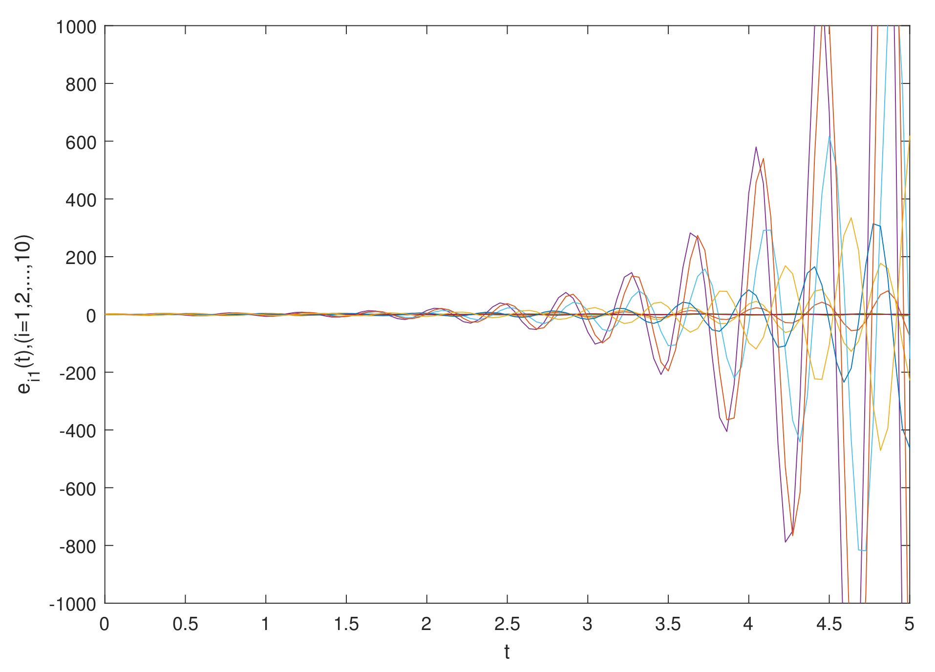
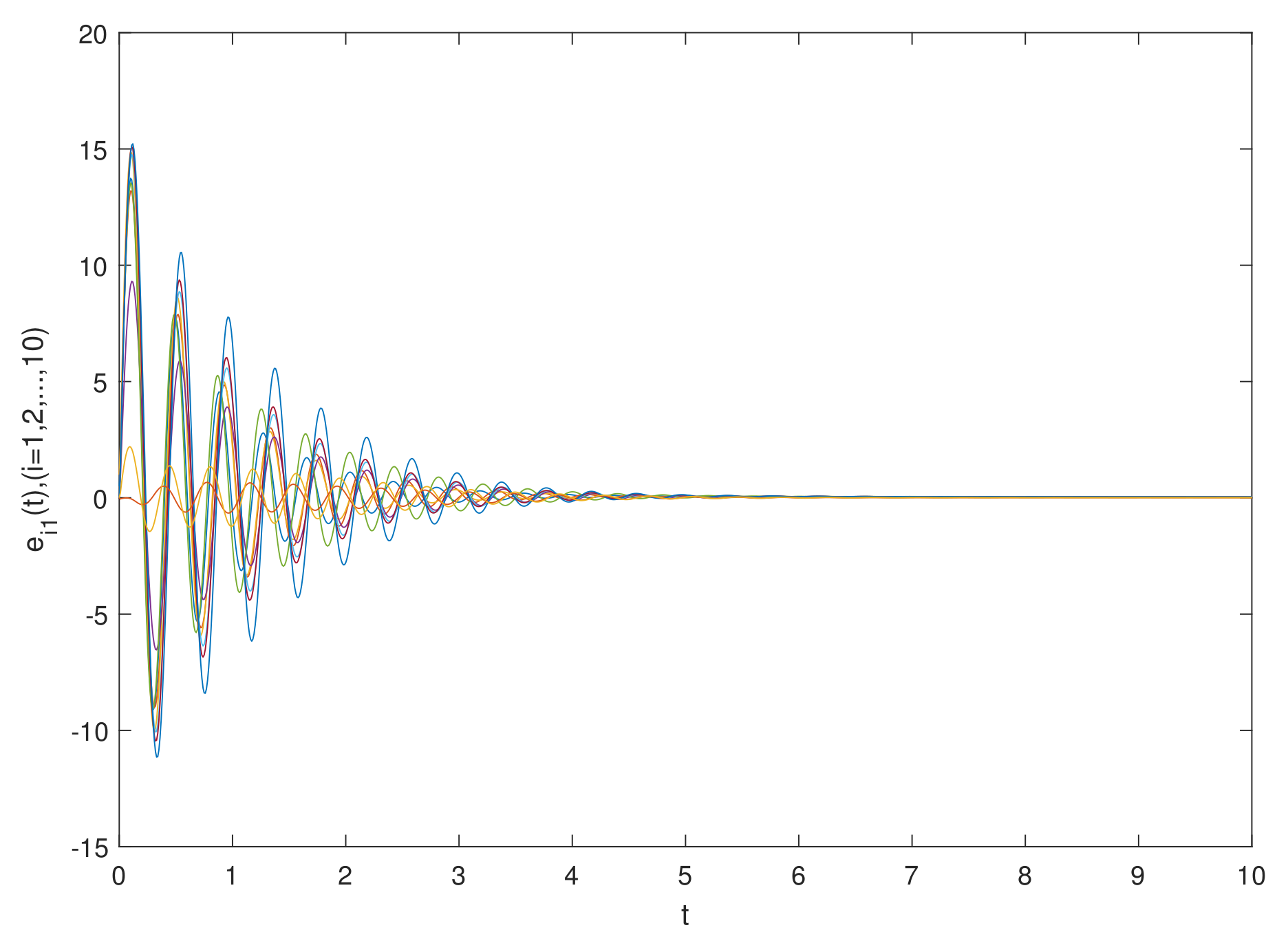
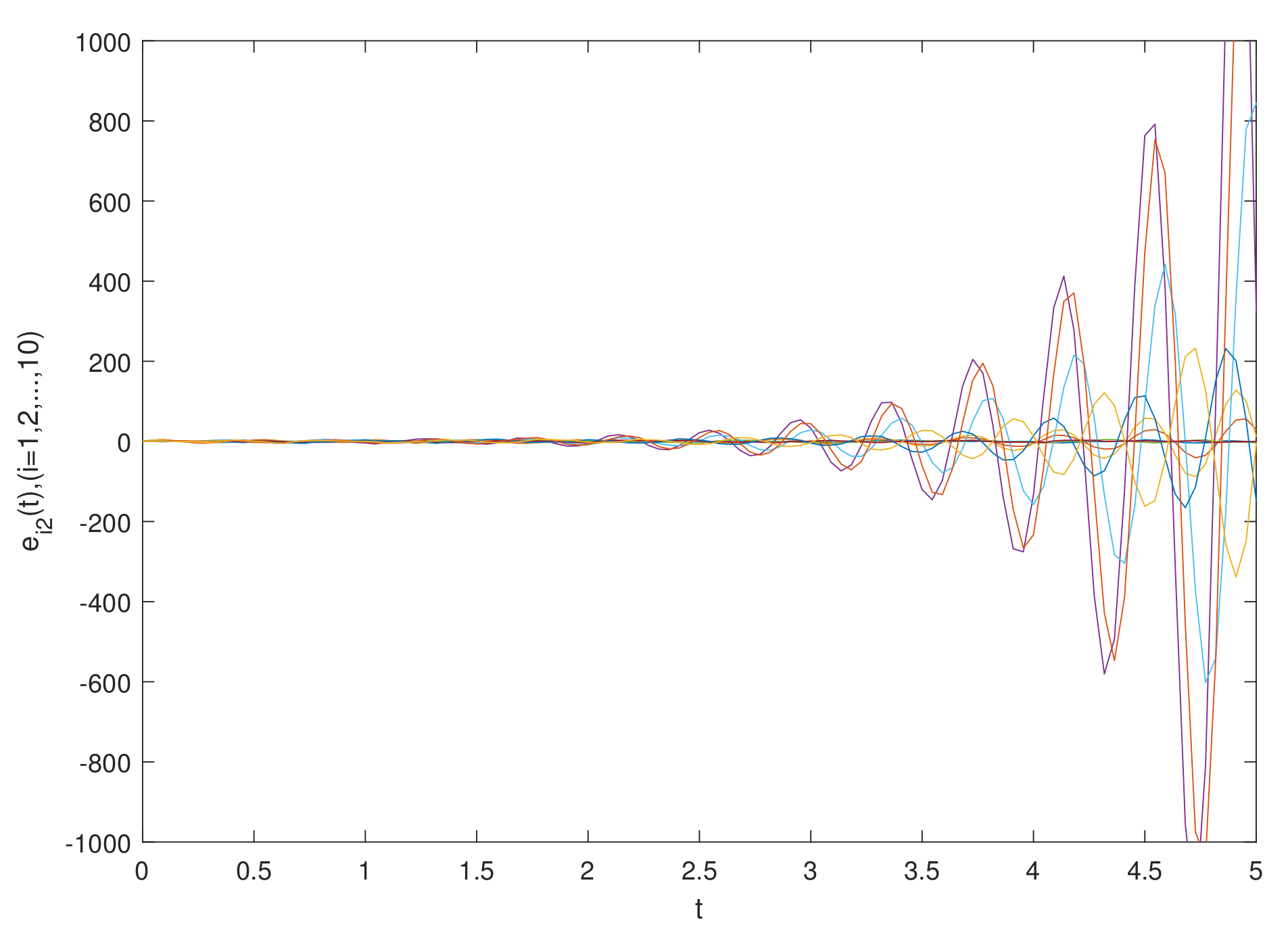
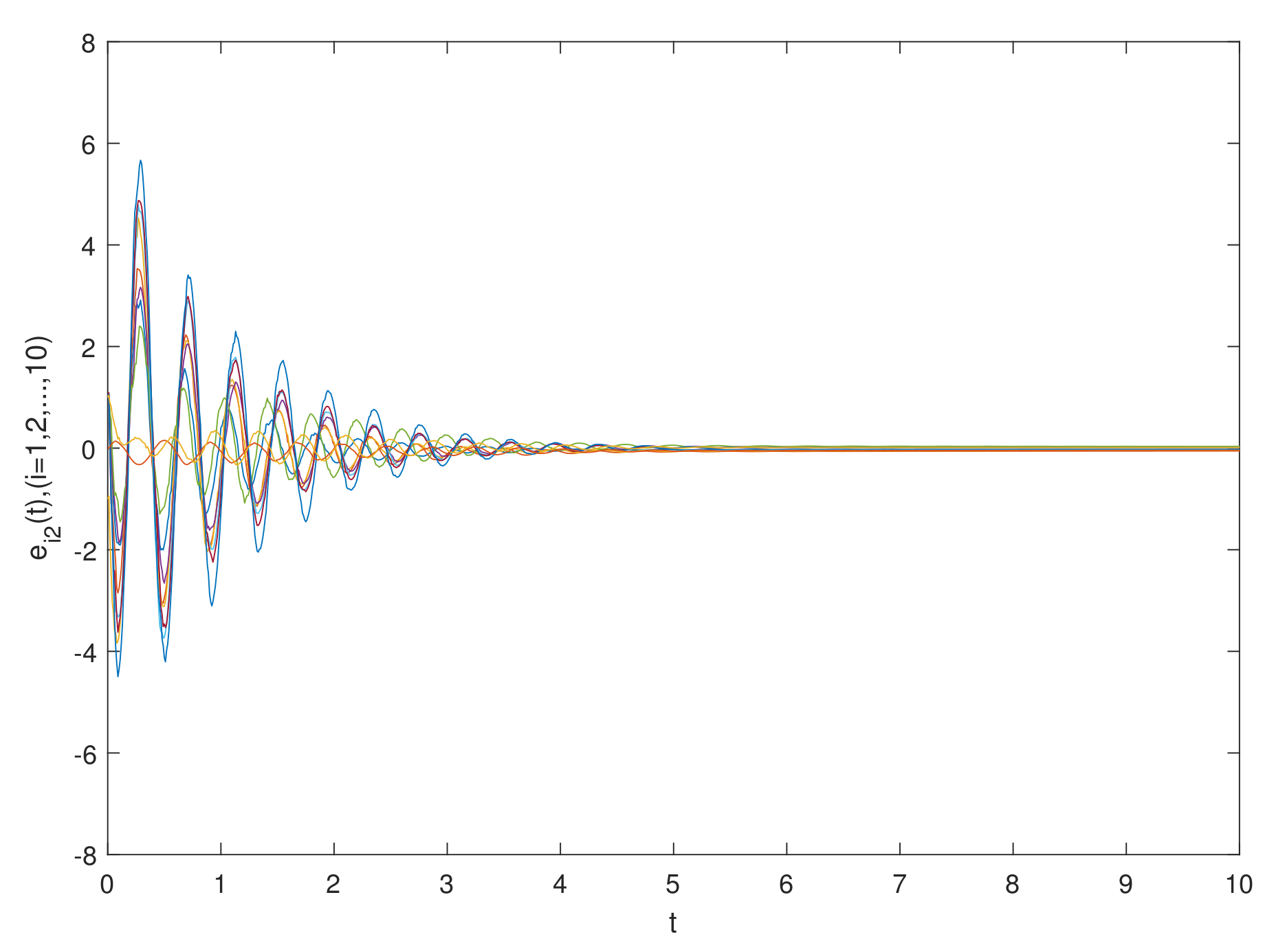
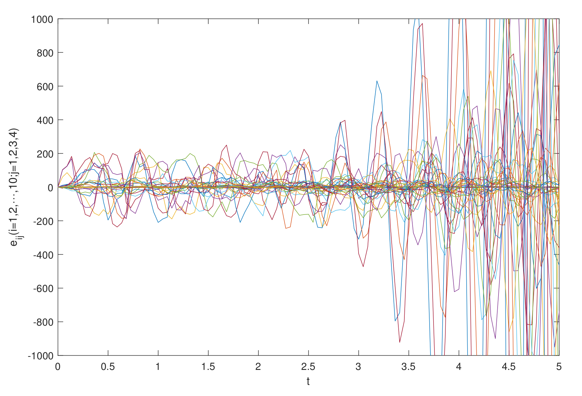
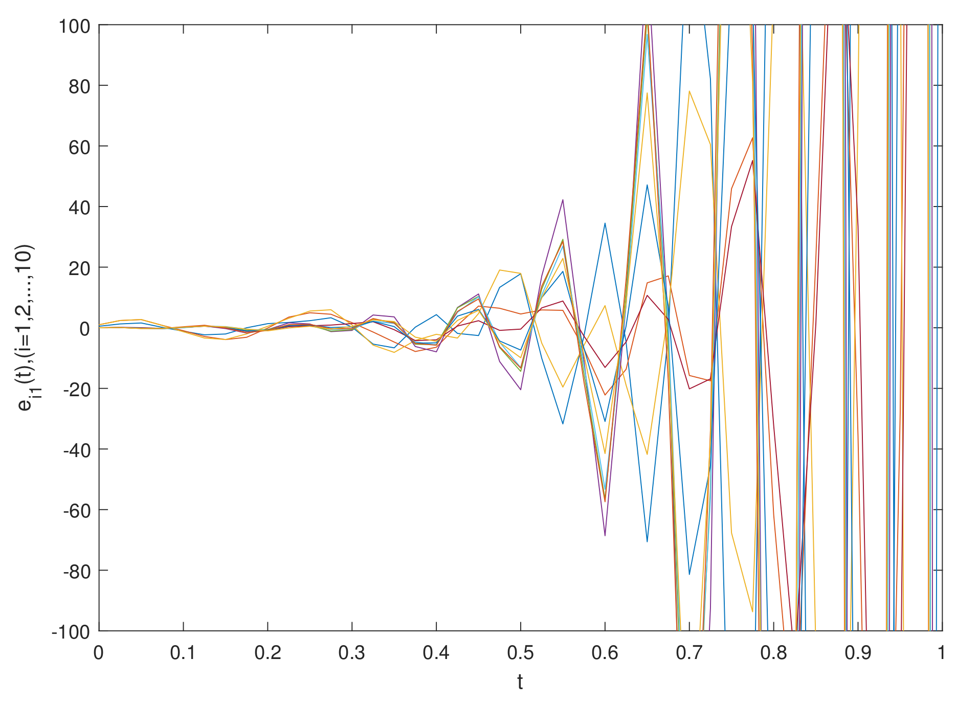
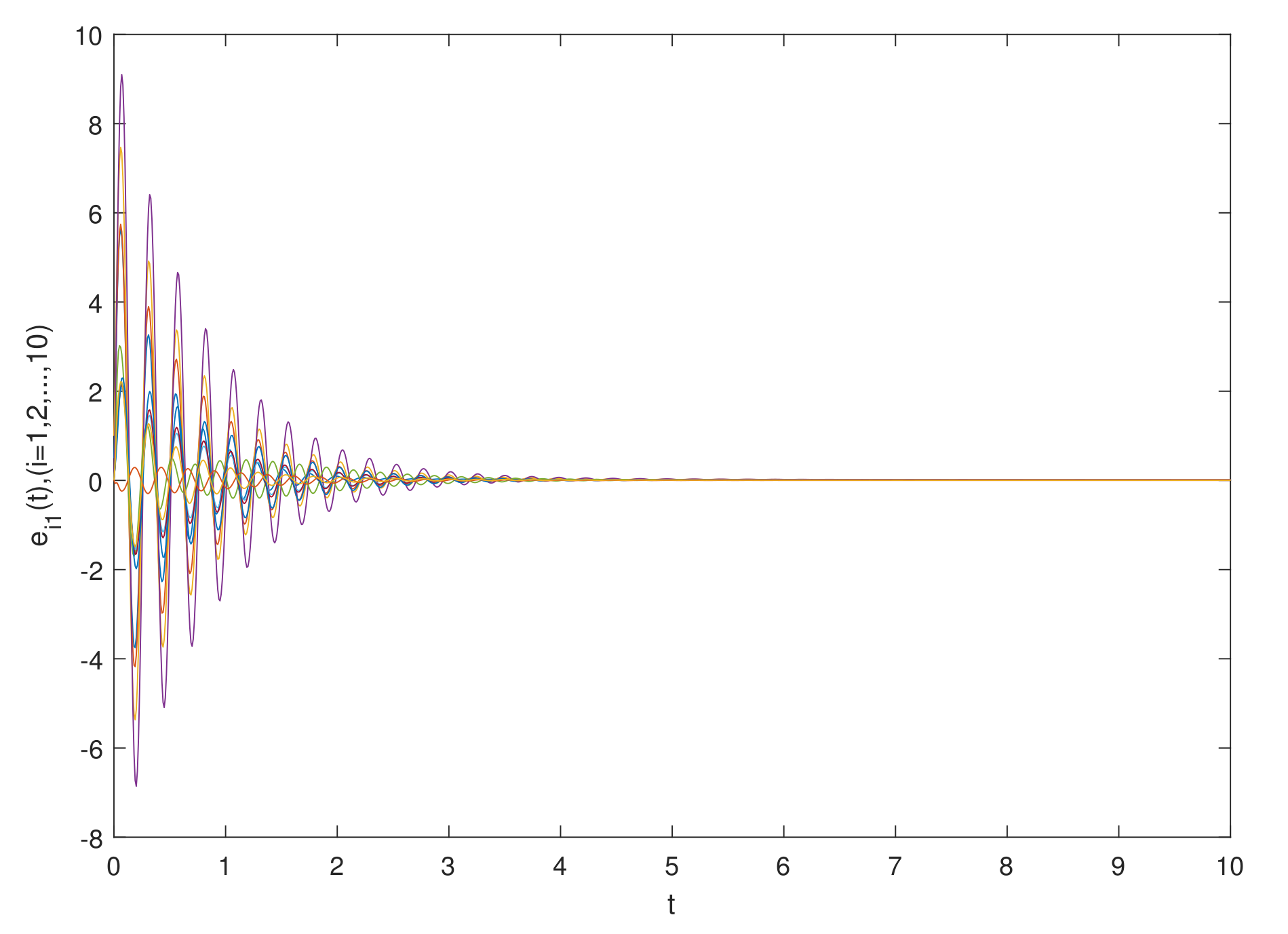
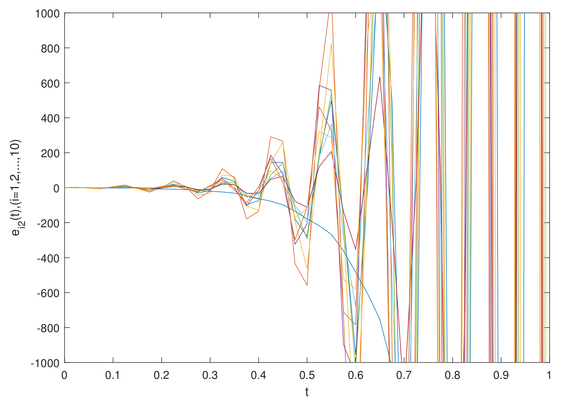
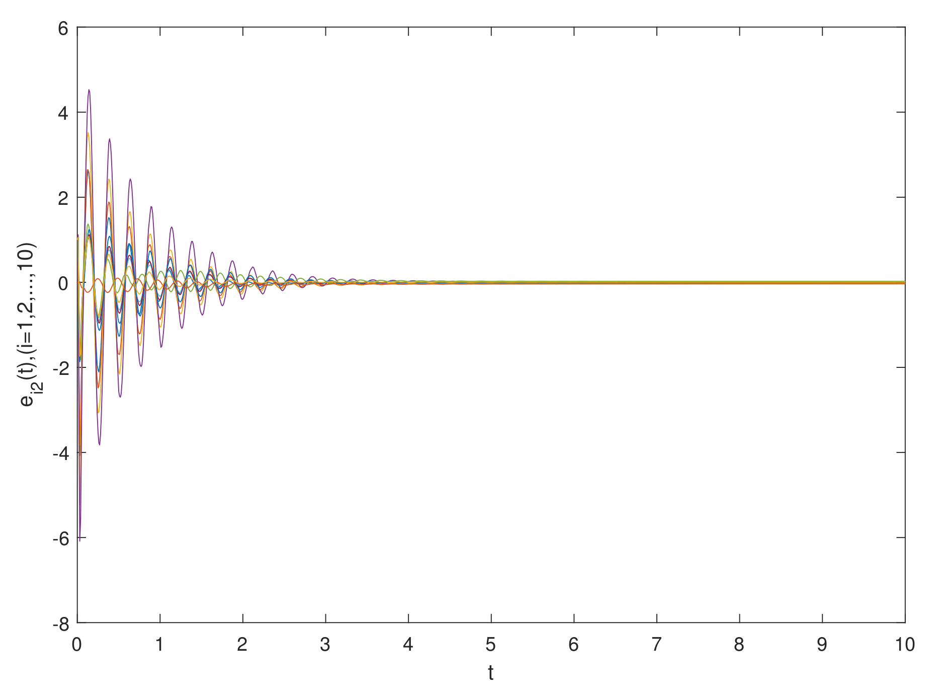
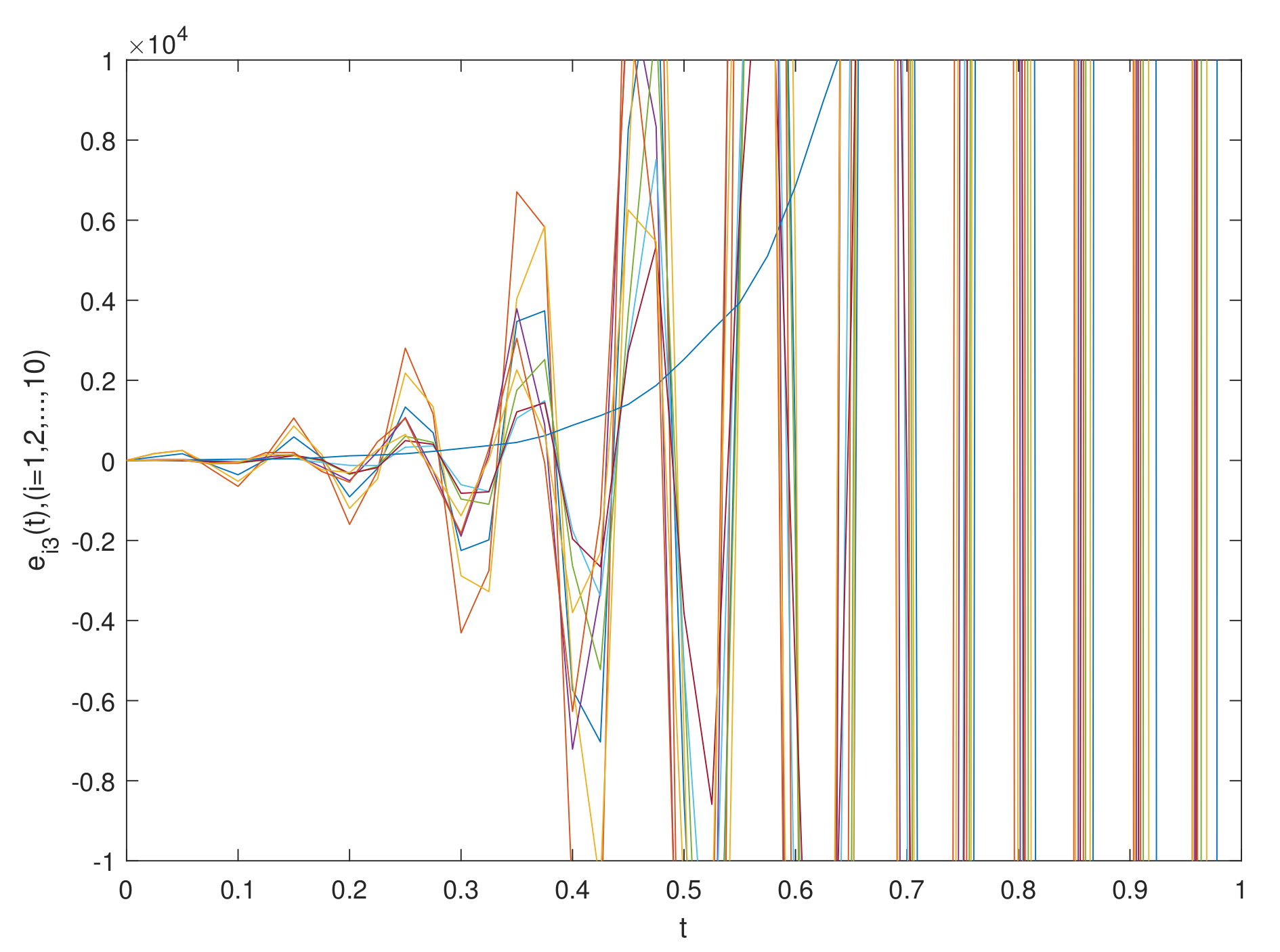
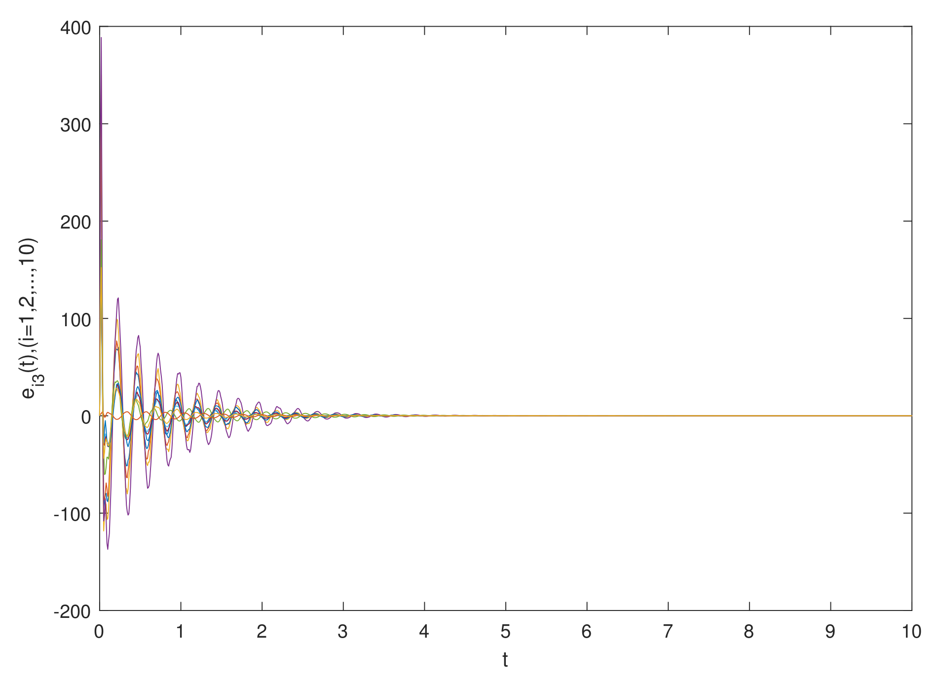
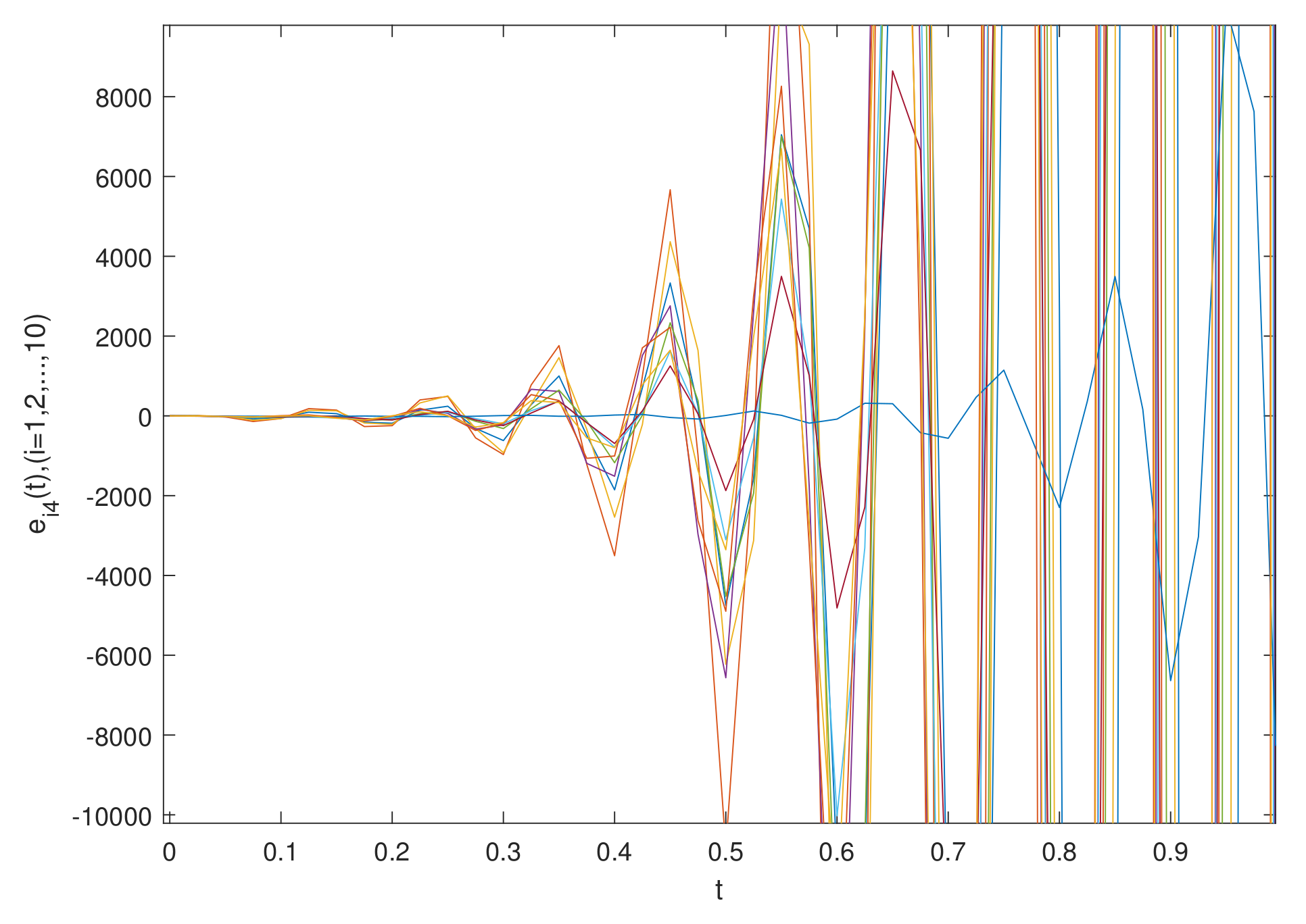
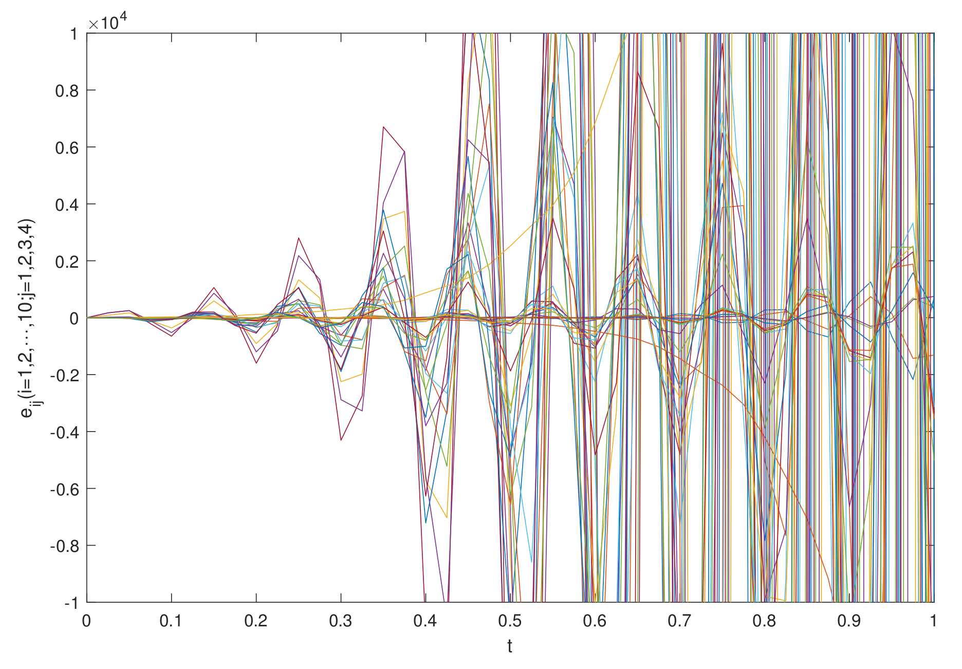
4. Numerical Simulation

In this part, two numerical instances are presented to illustrate the effectiveness of the proposed method.

Example 1.

Suppose that the following FCDNDP is composed of N nodes, and every node is a n-dimensional system which is given as follows

$$\begin{array}{c}\hfill {}_{t_0}^C{D}_t^{\xi }{\varphi }_p\left(t\right)=A{\varphi }_p\left(t\right)+B\gamma {\varphi }_p\left(t\right)+c\sum _{q=1}^N{d}_{pq}{\Lambda }_1{\varphi }_q\left(t\right),\end{array}$$

(32)

and

$$\begin{array}{c}\hfill {}_{t_0}^C{D}_t^{\xi }{\phi }_p\left(t\right)=(E_0+\Delta E){\phi }_p\left(t\right)+(G_0+\Delta G)\eta {\phi }_p\left(t\right)+k\sum _{q=1}^N{L}_{pq}{\Lambda }_2{\phi }_q\left(t\right)+{\omega }_p\left(t\right),\end{array}$$

(33)

where $p=1,2,3,4$. $c=0.01$; $k=0.02$; $\varsigma {\varphi }_p\left(t\right)=(0.25\ast tanh\left(x_1\left(t\right)\right),0.25\ast tanh\left(x_2\left(t\right)\right),0.25\ast tanh\left(x_3\left(t\right)\right),0.25\ast tanh\left(x_4\left(t\right)\right))$; $\eta {\phi }_p\left(t\right)=(8.10\ast tanh\left(x_1\left(t\right)\right),8.10\ast tanh\left(x_2\left(t\right)\right),8.10\ast$$tanh\left(x_3\left(t\right)\right),8.10\ast tanh\left(x_4\left(t\right)\right)).$

The parameter matrices and weight connection matrices can be expressed as

$$A=\left(\begin{array}{cccc}-20.15& 0& 0& 0\\ 0& -5.98& 0& 0\\ 0& 0& -12.47& 0\\ 0& 0& 0& -16.56\end{array}\right),B=\left(\begin{array}{cccc}0.2& 0& 0.5& 0.78\\ 0& -1.15& 1& 0.35\\ 0.3& 1& -1& 0\\ 0& 0& 0& -2.15\end{array}\right),$$

$$E=\left(\begin{array}{cccc}-2.14& 0& 0& 0\\ 0& -0.16& 0& 0\\ 0& 0& -5.57& 0\\ 0& 0& 0& -0.23\end{array}\right),D=\left(\begin{array}{cccc}1& 0.025& 0.1& 0.6\\ -2.1& 1& 0& 1\\ 0& -1& -2.25& 1\\ 1& 0& 1& -1.35\end{array}\right).$$

Meanwhile, the inner coupling matrices can be expressed as

$${\Lambda }_1=\left(\begin{array}{cccc}0.25& 0& 0& 0\\ 0& 0.25& 0& 0\\ 0& 0& 0.25& 0\\ 0& 0& 0& 0.25\end{array}\right),{\Lambda }_2=\left(\begin{array}{cccc}0.35& 0& 0& 0\\ 0& 0.35& 0& 0\\ 0& 0& 0.35& 0\\ 0& 0& 0& 0.35\end{array}\right).$$

The matrices of parameter uncertainties can be expressed as

$$H_1=\left(\begin{array}{cccc}0.1& 0& 0& 0\\ 0& 0.5& 0& 0\\ 0& 0& 0.2& 0\\ 0& 0& 0& 0.3\end{array}\right),K_1=\left(\begin{array}{cccc}0.2& 0& 0& 0\\ 0& 0.1& 0& 0\\ 0& 0& 0.2& 0\\ 0& 0& 0& 0.5\end{array}\right),$$

$${\Xi }_1=\left(\begin{array}{cccc}cos\left(x_1\left(t\right)\right)& 0& 0& 0\\ 0& cos\left(x_2\left(t\right)\right)& 0& 0\\ 0& 0& cos\left(x_3\left(t\right)\right)& 0\\ 0& 0& 0& cos\left(x_4\left(t\right)\right)\end{array}\right).$$

The external coupling matrices can be expressed as

$$d_{pq}=\left(\begin{array}{cccccccccc}-1& 0& 1.5& 0& 2.5& -2.1& 1& -1& 0.2& -2.25\\ -2& -1.5& 0& -0.2& 0.1& -0.5& 0& 1.5& 0.1& -3\\ 0& -1& -3& 0& 1& -1.5& 0& -1.25& -1.15& 1\\ 2.5& 0& 1.5& -2& 1.5& 0& -1.5& 0& -2& 0.5\\ 0& -1& 0& 1& -2.25& -1.45& -1.5& 3& 0.5& -1.1\\ -1.01& 0& 2& -2& 1& -1.5& 0& 1& -1& 0\\ 0.5& 0& -1& 2.1& 0& 1.5& -1.5& -1.5& 1.01& 1.45\\ -2& 0.1& -1.01& 1& -1.5& 0& -1& -1.45& 2.25& -0.2\\ 1& -2.5& 0& 1.5& -1& 0.2& 0.5& 1& -1.15& -1.25\\ 1.5& -3& 0.5& -0.5& 0& -1.15& 3& 0& 0.2& -1\end{array}\right),$$

$$L_{pq}=\left(\begin{array}{cccccccccc}-2& 0& 0& 1.5& -1.5& 3& -1& 0& 1& 0.5\\ -1& -1& 0& 1& -3.5& 0& 0.25& 2& 1.5& 0\\ 0& 1& -3.5& 0.5& 0.25& 0& 0& 1.5& -2.25& -0.5\\ 1& -1& -1.25& -0.15& 0& 1& 2& -2.5& 0& -1.5\\ -0.15& 2.25& -1& 0& -1& 2& 0& -0.15& 0.25& 3\\ 0& -0.26& -3& 0& 0& -1& 2& 1& -1& -1\\ -1.25& 0& 0.25& -1.25& 2& 0& -2.5& -0.15& 0& 0.25\\ 0& -1.5& 1& 0& 1& -2.25& 1.5& -1& 0.15& 0\\ 2.25& 1.25& 0& 1.5& 0.5& 1& -1& 0& -0.25& -2\\ -0.5& 0& 1& -2& 0& 0.5& -3& 1& 0& -1.5\end{array}\right).$$

The simulation results are shown in Figure 1 and Figure 2, which show the time waveforms of the system errors $e_{i1}$. Figure 1 shows the variation of the synchronization error system without a controller. Figure 2 shows the variation of the synchronization error system with a controller. Figure 3, Figure 4, Figure 5, Figure 6, Figure 7, Figure 8, Figure 9 and Figure 10 show the variation in the synchronization error systems $e_{i2},e_{i3},e_{i4},e_{ij}(i=1,2,···,10;j=1,2,3,4)$. According to the simulation results and figures, one can obtain that the error system is driven to initial point, i.e., the FCDNDP is synchronized, which verifies the validity of the proposed controller.

Example 2.

Suppose that the following FCDNDP is composed of N nodes and every node is a n-dimensional system, which is given as follows

$$\begin{array}{c}\hfill {}_{t_0}^C{D}_t^{\xi }{\varphi }_p\left(t\right)=A{\varphi }_p\left(t\right)+B\gamma {\varphi }_p\left(t\right)+c\sum _{q=1}^N{d}_{pq}{\Lambda }_1{\varphi }_q\left(t\right),\end{array}$$

(34)

and

$$\begin{array}{c}\hfill {}_{t_0}^C{D}_t^{\xi }{\phi }_p\left(t\right)=(E_0+\Delta E){\phi }_p\left(t\right)+(G_0+\Delta G)\eta {\phi }_p\left(t\right)+k\sum _{q=1}^N{L}_{pq}{\Lambda }_2{\phi }_q\left(t\right)+{\omega }_p\left(t\right).\end{array}$$

(35)

The parameter matrices and weight connection matrices can be expressed as

$$A=\left(\begin{array}{cccc}-30.15& 0& 0& 0\\ 0& -7.99& 0& 0\\ 0& 0& -15.73& 0\\ 0& 0& 0& -24.89\end{array}\right),B=\left(\begin{array}{cccc}1& 0& 0.5& 0.35\\ 0& -2.15& 1& 0.35\\ 0& 1& -1& 0\\ 0& 0& 0& -0.15\end{array}\right),$$

$$E=\left(\begin{array}{cccc}-3.15& 0& 0& 0\\ 0& -0.52& 0& 0\\ 0& 0& -8.51& 0\\ 0& 0& 0& -0.45\end{array}\right),D=\left(\begin{array}{cccc}-1.048& 0.025& 0.1& 0.6\\ -2.1& 0.85& 0& 1.87\\ 0& -1& -3.25& -1\\ 1.86& 0& 1& -1.35\end{array}\right).$$

Meanwhile, the inner coupling matrices can be expressed as

$${\Lambda }_1=\left(\begin{array}{cccc}0.25& 0& 0& 0\\ 0& 0.25& 0& 0\\ 0& 0& 0.25& 0\\ 0& 0& 0& 0.25\end{array}\right),{\Lambda }_2=\left(\begin{array}{cccc}0.35& 0& 0& 0\\ 0& 0.35& 0& 0\\ 0& 0& 0.35& 0\\ 0& 0& 0& 0.35\end{array}\right).$$

The matrices of parameter uncertainties can be expressed as

$$H_2=\left(\begin{array}{cccc}1& 0& 0& 0\\ 0& 0.9& 0& 0\\ 0& 0& 1& 0\\ 0& 0& 0& 0.3\end{array}\right),K_1=\left(\begin{array}{cccc}1& 0& 0& 0\\ 0& 0.9& 0& 0\\ 0& 0& 0.8& 0\\ 0& 0& 0& 1\end{array}\right),$$

$${\Xi }_2=\left(\begin{array}{cccc}0.41cos\left(x_1\left(t\right)\right)& 0& 0& 0\\ 0& cos\left(x_2\left(t\right)\right)& 0& 0\\ 0& 0& 0.3cos\left(x_3\left(t\right)\right)& 0\\ 0& 0& 0& 0.13cos\left(x_4\left(t\right)\right)\end{array}\right).$$

The external coupling matrices can be expressed as

$$d_{pq}=\left(\begin{array}{cccccccccc}-1& 0& 1.5& 0& 2.5& -2.1& 1& -1& 0.2& -2.25\\ -2& -1.5& 0& -0.2& 0.1& -0.5& 0& 1.5& 0.1& -3\\ 0& -1& -3& 0& 1& -1.5& 0& -1.25& -1.15& 1\\ 2.5& 0& 1.5& -2& 1.5& 0& -1.5& 0& -2& 0.5\\ 0& -1& 0& 1& -2.25& -1.45& -1.5& 3& 0.5& -1.1\\ -1.01& 0& 2& -2& 1& -1.5& 0& 1& -1& 0\\ 0.5& 0& -1& 2.1& 0& 1.5& -1.5& -1.5& 1.01& 1.45\\ -2& 0.1& -1.01& 1& -1.5& 0& -1& -1.45& 2.25& -0.2\\ 1& -2.5& 0& 1.5& -1& 0.2& 0.5& 1& -1.15& -1.25\\ 1.5& -3& 0.5& -0.5& 0& -1.15& 3& 0& 0.2& -1\end{array}\right),$$

$$L_{pq}=\left(\begin{array}{cccccccccc}-2& 0& 0& 1.5& -1.5& 3& -1& 0& 1& 0.5\\ -1& -1& 0& 1& -3.5& 0& 0.25& 2& 1.5& 0\\ 0& 1& -3.5& 0.5& 0.25& 0& 0& 1.5& -2.25& -0.5\\ 1& -1& -1.25& -0.15& 0& 1& 2& -2.5& 0& -1.5\\ -0.15& 2.25& -1& 0& -1& 2& 0& -0.15& 0.25& 3\\ 0& -0.26& -3& 0& 0& -1& 2& 1& -1& -1\\ -1.25& 0& 0.25& -1.25& 2& 0& -2.5& -0.15& 0& 0.25\\ 0& -1.5& 1& 0& 1& -2.25& 1.5& -1& 0.15& 0\\ 2.25& 1.25& 0& 1.5& 0.5& 1& -1& 0& -0.25& -2\\ -0.5& 0& 1& -2& 0& 0.5& -3& 1& 0& -1.5\end{array}\right).$$

Meanwhile, the other parameters are the same as in Example 1.

The simulation results are shown in Figure 11 and Figure 12, which show the time waveforms of the system errors $e_{i1}$. Figure 11 shows the variation in the synchronization error system without a controller. Figure 12 shows the variation in the synchronization error system with a controller. Figure 13, Figure 14, Figure 15, Figure 16, Figure 17, Figure 18, Figure 19 and Figure 20 shows the variation in synchronization error systems $e_{i2},e_{i3},e_{i4},e_{ij}(i=1,2,···,10;j=1,2,3,4)$. According to the simulation results and figures, one can obtain that the error system is driven to the initial point, i.e., the FCDNDP is synchronized, which verifies the validity of the proposed controller.

5. Conclusions

In this paper, by applying the fractional differential equation theory and differential inclusion theory, a driving response system with different structures is established. The driving system is a general driving model, and the response system is a response model with parameter uncertainties. Based on the Lyapunov direct method, a sufficient condition for the asymptotic synchronization of FCDNDP is established. When we deal with a similar problem, this method can ensure that the obtained results have better application and less conservatism. Finally, the validity and feasibility of the theoretical outcomes are confirmed by two simulation instances. In the future, we hope to extend the technique proposed in this paper to the asymptotic synchronization of FCDNDP with time delay.

References

1. Podlubny, I. Fractional Differential Equations; Academic Press: San Diego, CA, USA, 1999. [Google Scholar]
2. Hilfer, R. Applications of Fractional Calculus in Physics; World Scientific: Hackensack, NJ, USA, 2000. [Google Scholar]
3. Bagley, R.L. On the Fractional Calculus Model of Viscoelastic Behavior. J. Rheol. 1998, 30, 133–155. [Google Scholar] [CrossRef]
4. Ge, Z.M.; Jhuang, W.R. Chaos, control and synchronization of a fractional order rotational mechanical system with a centrifugal governor. Chaos Solitons Fractals 2007, 33, 270–289. [Google Scholar] [CrossRef]
5. Huang, L.L.; He, S.J. Stability of fractional state space system and its application to fractional order chaotic system. Acta Phys. Sin. Chin. Ed. 2011, 60, 119419573. [Google Scholar] [CrossRef]
6. Hudson, J.L.; Kube, M.; Adomaitis, R.A.; Kevrekidis, I.G.; Lapedes, A.S.; Farber, R.M. Nonlinear signal processing and system identification: Applications to time series from electrochemical reactions. Chem. Eng. Sci. 1990, 45, 2075–2081. [Google Scholar] [CrossRef]
7. Argenti, F.; De Angeli, A.; Del Re, E.; Genesio, R.; Pagni, P.; Tesi, A. Secure communications based on discrete time chaotic systems. Kybernetika 1997, 1, 41–50. [Google Scholar]
8. Gerhards, M.; Schlerf, M.; Rascher, U.; Udelhoven, T.; Juszczak, R.; Alberti, G.; Miglietta, F.; Inoue, Y. Analysis of Airborne Optical and Thermal Imagery for Detection of Water Stress Symptoms. Remote Sens. 2018, 10, 1139. [Google Scholar] [CrossRef]
9. Lei, Y.; Zheng, W. Research on robot automation and control problems. World Inverters 2015, 3, 86–88. [Google Scholar]
10. Boccaletti, S.; Latora, V.; Moreno, Y.; Chavez, M.; Hwang, D.U. Complex networks: Structure and dynamics. Phys. Rep. 2006, 424, 175–308. [Google Scholar] [CrossRef]
11. Wang, Z.; Shu, H.; Liu, Y.; Ho, D.W.; Liu, X. Robust stability analysis of generalized neural networks with discrete and distributed time delays. Chaos Solitons Fractals 2006, 30, 886–896. [Google Scholar] [CrossRef]
12. Barabâsi, A.L.; Jeong, H.; Néda, Z.; Ravasz, E.; Schubert, A.; Vicsek, T. Evolution of the social network of scientific collaborations. Phys. Astatistical Mech. Its Appl. 2002, 311, 590–614. [Google Scholar] [CrossRef]
13. Melián, C.J.; Bascompte, J.; Jordano, P.; Krivan, V. Diversity in a complex ecological network with two interaction types. Oikos 2010, 118, 122–130. [Google Scholar] [CrossRef]
14. Zio, E.; Golea, L.R.; Mrs, C. Identifying groups of critical edges in a realistic electrical network by multi-objective genetic algorithms. Reliab. Eng. Syst. Saf. 2012, 99, 172–177. [Google Scholar] [CrossRef]
15. Ma, T.; Zhang, J. Hybrid synchronization of coupled fractional-order complex networks. Neurocomputing 2015, 157, 166–172. [Google Scholar] [CrossRef]
16. Li, H.L.; Cao, J.; Hu, C.; Zhang, L.; Wang, Z. Global synchronization between two fractional-order complex networks with non-delayed and delayed coupling via hybrid impulsive control. Neurocomputing 2019, 356, 31–39. [Google Scholar] [CrossRef]
17. Yang, L.X.; Jiang, J. Adaptive synchronization of drive-response fractional-order complex dynamical networks with uncertain parameters. Commun. Nonlinear Sci. Numer. Simul. 2014, 19, 1496–1506. [Google Scholar] [CrossRef]
18. Zhu, D.; Wang, R.; Liu, C.; Duan, J. Projective synchronization via adaptive pinning control for fractional-order complex network with time-varying coupling strength. Int. J. Mod. Phys. C 2019, 30, 268–968. [Google Scholar] [CrossRef]
19. Li, H.L.; Cao, J.; Jiang, H.; Alsaedi, A. Graph theory based finite-time synchronization of fractional-order complex dynamical networks. J. Frankl. Inst. 2018, 355, 5771–5789. [Google Scholar] [CrossRef]
20. Wu, H.; Wang, L.; Niu, P.; Wang, Y. Global projective synchronization in finite time of nonidentical fractional-order neural networks based on sliding mode control strategy. Neurocomputing 2017, 235, 264–273. [Google Scholar] [CrossRef]
21. Lin, D.U.; Yong, Y.; Lei, Y. Synchronization in a fractional-order dynamic network with uncertain parameters using an adaptive control strategy. Appl. Math. Mech. 2018, 39, 353–364. [Google Scholar]
22. Shen, Y.; Li, C. LMI-based finite-time boundedness analysis of neural networks with parametric uncertainties. Neurocomputing 2008, 71, 502–507. [Google Scholar] [CrossRef]
23. Wong, W.K.; Li, H.; Leung, S. Robust synchronization of fractional-order complex dynamical networks with parametric uncertainties. Commun. Nonlinear Sci. Numer. Simul. 2012, 17, 4877–4890. [Google Scholar] [CrossRef]
24. Li, H.J. State Estimation for Fractional-Order Complex Dynamical Networks with Linear Fractional Parametric Uncertainty. Abstr. Appl. Anal. 2013, 2013, 151–164. [Google Scholar] [CrossRef]
25. Samli, R.; Yucel, E. Global robust stability analysis of uncertain neural networks with time varying delays. Neurocomputing 2015, 167, 371–377. [Google Scholar] [CrossRef]
26. Ding, Z.; Shen, Y. Projective synchronization of nonidentical fractional-order neural networks based on sliding mode controller. Neural Netw. 2016, 76, 97–105. [Google Scholar] [CrossRef]
27. Hu, T.; Zhang, X.; Zhong, S. Global asymptotic synchronization of nonidentical fractional-order neural networks. Neurocomputing 2018, 313, 39–46. [Google Scholar] [CrossRef]
28. Suntonsinsoungvon, E.; Udpin, S. Exponential stability of discrete-time uncertain neural networks with multiple time-varying leakage delays. Math. Comput. Simul. 2020, 171, 233–245. [Google Scholar] [CrossRef]
29. Aadhithiyan, S.; Raja, R.; Kou, B.; Selvam, G.; Niezabitowski, M.; Lim, C.P.; Cao, J. Asymptotic synchronization of fractional order non-identical complex dynamical networks with Parameter Uncertainties. Math. Methods Appl. Sci. 2022, 2022, 1–19. [Google Scholar] [CrossRef]
30. Wei, J.; Pan, G. Design of a Sliding Mode Controller for Synchronization of Fractional-Order Chaotic Systems with Different Structures. J. Shanghai Jiaotong Univ. 2016, 50, 849–853, 860. [Google Scholar]
31. Zeng, H.B.; He, Y.; Wu, M.; Xiao, H.Q. Improved Conditions for Passivity of Neural Networks With a Time-Varying Delay. IEEE Trans. Cybern. 2014, 44, 785–792. [Google Scholar] [CrossRef]
Figure 1. Synchronization errors e i 1 ( i = 1 , 2 , · · · , 10 ) of the fractional-order system (32) and (33) without the controllers.
Fractalfract 06 00441 g001
Figure 2. Synchronization errors e i 1 ( i = 1 , 2 , · · · , 10 ) of the fractional-order system (32) and (33) with the controllers.
Fractalfract 06 00441 g002
Figure 3. Synchronization errors e i 2 ( i = 1 , 2 , · · · , 10 ) of the fractional-order system (32) and (33) without the controllers.
Fractalfract 06 00441 g003
Figure 4. Synchronization errors e i 2 ( i = 1 , 2 , · · · , 10 ) of the fractional-order system (32) and (33) with the controllers.
Fractalfract 06 00441 g004
Figure 5. Synchronization errors e i 3 ( i = 1 , 2 , · · · , 10 ) of the fractional-order system (32) and (33) without the controllers.
Fractalfract 06 00441 g005
Figure 6. Synchronization errors e i 3 ( i = 1 , 2 , · · · , 10 ) of the fractional-order system (32) and (33) with the controllers.
Fractalfract 06 00441 g006
Figure 7. Synchronization errors e i 4 ( i = 1 , 2 , · · · , 10 ) of the fractional-order system (32) and (33) without the controllers.
Fractalfract 06 00441 g007
Figure 8. Synchronization errors e i 4 ( i = 1 , 2 , · · · , 10 ) of the fractional-order system (32) and (33) with the controllers.
Fractalfract 06 00441 g008
Figure 9. Synchronization errors e i j ( i = 1 , 2 , · · · , 10 ; j = 1 , 2 , 3 , 4 ) of the fractional-order system (32) and (33) without the controllers.
Fractalfract 06 00441 g009
Figure 10. Synchronization errors e i j ( i = 1 , 2 , · · · , 10 ; j = 1 , 2 , 3 , 4 ) of the fractional-order system (32) and (33) with the controllers.
Fractalfract 06 00441 g010
Figure 11. Synchronization errors e i 1 ( i = 1 , 2 , · · · , 10 ) of the fractional-order system (34) and (35) without the controllers.
Fractalfract 06 00441 g011
Figure 12. Synchronization errors e i 1 ( i = 1 , 2 , · · · , 10 ) of the fractional-order system (34) and (35) with the controllers.
Fractalfract 06 00441 g012
Figure 13. Synchronization errors e i 2 ( i = 1 , 2 , · · · , 10 ) of the fractional-order system (34) and (35) without the controllers.
Fractalfract 06 00441 g013
Figure 14. Synchronization errors e i 2 ( i = 1 , 2 , · · · , 10 ) of the fractional-order system (34) and (35) with the controllers.
Fractalfract 06 00441 g014
Figure 15. Synchronization errors e i 3 ( i = 1 , 2 , · · · , 10 ) of the fractional-order system (34) and (35) without the controllers.
Fractalfract 06 00441 g015
Figure 16. Synchronization errors e i 3 ( i = 1 , 2 , · · · , 10 ) of the fractional-order system (34) and (35) with the controllers.
Fractalfract 06 00441 g016
Figure 17. Synchronization errors e i 4 ( i = 1 , 2 , · · · , 10 ) of the fractional-order system (34) and (35) without the controllers.
Fractalfract 06 00441 g017
Figure 18. Synchronization errors e i 4 ( i = 1 , 2 , · · · , 10 ) of the fractional-order system (34) and (35) with the controllers.
Fractalfract 06 00441 g018
Figure 19. Synchronization errors e i j ( i = 1 , 2 , · · · , 10 ; j = 1 , 2 , 3 , 4 ) of the fractional-order system (34) and (35) without the controllers.
Fractalfract 06 00441 g019
Figure 20. Synchronization errors e i j ( i = 1 , 2 , · · · , 10 ; j = 1 , 2 , 3 , 4 ) of the fractional-order system (34) and (35) with the controllers.
Fractalfract 06 00441 g020
Publisher’s Note: MDPI stays neutral with regard to jurisdictional claims in published maps and institutional affiliations.