Application of the Explicit Euler Method for Numerical Analysis of a Nonlinear Fractional Oscillation Equation

Abstract

In this paper, a numerical analysis of the oscillation equation with a derivative of a fractional variable Riemann–Liouville order in the dissipative term, which is responsible for viscous friction, is carried out. Using the theory of finite-difference schemes, an explicit finite-difference scheme (Euler’s method) was constructed on a uniform computational grid. For the first time, the issues of approximation, stability and convergence of the proposed explicit finite-difference scheme are considered. To compare the results, the Adams–Bashford–Moulton scheme was constructed as an experimental method. The theoretical results were confirmed using test examples, the computational accuracy of the method was evaluated, which is consistent with the theoretical one, and the simulation results were visualized. Using the example of a fractional Duffing oscillator, waveforms and phase trajectories, as well as its amplitude–frequency characteristics, were constructed using a finite-difference scheme. To identify chaotic regimes, the spectra of maximum Lyapunov exponents and Poincaré points were constructed. It is shown that an explicit finite-difference scheme can be acceptable under the condition of a step of the computational grid.

1. Introduction

Currently, the use of fractional calculus in the theory of dissipative oscillatory systems to describe dynamic memory has been widely developed [1]. Dynamic memory in a dissipative oscillatory system is due to the ability of the system to “remember” the impact on it—the impulse of the system, which is gradually “forgotten”.

It should be noted that the effects of dynamic memory, for example, are considered within the framework of hereditary mechanics to describe viscoelastic and plastic media [2].

As the authors of [3,4,5,6] have shown, the transition from ordinary differential equations to differential equations with derivatives of fractional orders describes the effects of heredity in dissipative oscillatory systems quite well, and the orders of fractional derivatives are associated with their qualitative characteristic—the Q-factor, as well as with amplitude–frequency and phase–frequency characteristics.

A mathematical model of an oscillatory system (oscillator), in which derivatives of fractional orders are included, is called fractional oscillators in the literature [3]. In [1], the rest points of the various nonlinear fractional oscillators of Duffing, Van der Pol, etc., were investigated. Here, waveforms and phase trajectories were constructed, using numerical methods that have not been studied for stability and convergence.

In [7,8,9,10,11,12,13,14,15], a fractional Duffing oscillator with a Riemann–Liouville derivative of constant fractional order in the dissipative term was investigated, and regular and chaotic modes were investigated using numerical analysis—the theory of finite-difference schemes. It should also be noted that studies of the fractional Duffing oscillator were carried out using the HAM method [16], as well as using power series expansion [17].

An approximate analytical solution was found for the Duffing oscillator in terms of exponential and trigonometric functions [18]. Additionally, in [18], the analytical solution was compared with the numerical one obtained by the Runge–Kutta method. In ref. [19], analytical formulas were given for the starting point of the unstable solution domain for forced oscillations of the Duffing system, taking into account damping. Using the standard deviation estimation method based on the Poincaré cross section, a quantitative assessment of the chaotic state in [20] was implemented.

In refs. [21,22], the fractional Duffing oscillator was generalized to the case of the Riemann–Liouville derivative of non-constant fractional order; waveforms and phase trajectories were constructed using finite difference theory; and regular and chaotic regimes were investigated using the spectra of maximum Lyapunov exponents.

Unfortunately, the works listed above did not provide a rigorous substantiation of the issues of stability and convergence. Therefore, this work aims to fill this gap. The scientific novelty of this work is that for the first time, the stability and convergence theorem of an explicit finite-difference scheme are proved. There are no rigorous studies of a non-local explicit finite-difference scheme in the scientific literature (the stability and convergence theorems have not been proven). Theoretical results were confirmed by concrete test cases and computer simulations. The developed numerical algorithm is further used in the framework of qualitative analysis of the Duffing oscillator. Its chaotic and regular modes are investigated using bifurcation diagrams (spectra of maximum Lyapunov exponents), the amplitude–frequency response, and Poincaré sections are also calculated. It is shown that the numerical algorithm can be used to study such systems.

The work is organized as follows. Section 2 provides preliminary information. Section 3 presents the problem statement. Section 4 considers a numerical method for solving the formulated problem based on a nonlocal explicit finite difference scheme (explicit Euler’s method). Section 5 considers the issues of stability and convergence of a nonlocal explicit finite difference scheme. Section 6 presents the Adams–Bashford–Moulton numerical method for solving the formulated Cauchy problem. Section 7 gives detailed examples of the operation, the proposed numerical scheme, and an example of a numerical study of the fractional Duffing oscillator, as well as the amplitude–frequency response. In Section 8, chaotic modes of the Duffing system are investigated, and the spectra of maximum Lyapunov exponents and Poincaré points are constructed. Section 9 provides conclusions based on the results of the study.

2. Preliminaries

Here are some data from the theory of fractional calculus [23,24].

Let $x\left(t\right)\in C^2\left(0,T\right)$, $q\left(t\right)\in C\left(0,T\right)$, $t\in [0,T]$ be the current time and $T>0$ be the time of the process under consideration, then we will introduce into consideration the definition of the derivative of a fractional variable order of Riemann–Liouville.

Definition 1.

The Riemann–Liouville derivative of fractional variable order $0<q\left(t\right)<1$ has the following form:

$$D_{0t}^{q\left(t\right)}x\left(t\right)=\frac{1}{\mathsf{\Gamma }\left(1-q\left(t\right)\right)}\frac{d}{dt}\underset{0}{\overset{t}{\int }}\frac{x\left(\tau \right)d\tau }{{\left(t-\tau \right)}^{q\left(t\right)}},$$

(1)

where $\mathsf{\Gamma }\left(1-q\left(t\right)\right)$ is Euler’s gamma function, calculated using the formula $\mathsf{\Gamma }\left(y+1\right)=\underset{0}{\overset{\propto }{\int }}{x}^y{e}^{-x}dx$.

In the future, to construct a finite-difference scheme, we will need a discrete analog of the fractional derivative (1)—the Grunwald–Letnikov derivative.

Definition 2.

The Grunwald–Letnikov derivative of fractional variable order $0<q\left(t\right)<1$ has the form [25]

$${\Delta }_{0t}^{q\left(t\right)}x\left(t\right)=\underset{T⟶\propto }{lim}\frac{1}{h^{q\left(t\right)}}{\displaystyle \sum _{i=0}^T}{c}_i^{q\left(t\right)}x(t-ih),$$

(2)

where $c_i^{q\left(t\right)}=\frac{{(-1)}^i\mathsf{\Gamma }(1+q\left(t\right))}{\mathsf{\Gamma }(i+1)\mathsf{\Gamma }(i-q(t)-1)}$ are the Grunwald–Letnikov weight coefficients, and h is the sampling step.

Remark 1.

Sometimes the weights $c_i^{q\left(t\right)}$ are written differently:

$$c_i^{q\left(t\right)}=\left(1-\frac{1+q\left(t\right)}{i}\right)c_{i-1}^{q\left(t\right)},c_0^{q\left(t\right)}=1.$$

(3)

It can be shown that the entries of the weighting coefficients in (2) and (3) are equivalent.

Remark 2.

In the article, we used a well-known approach, for example, considered in the works [25,26]. According to this approach, the relationship between the Riemann–Liouville (1) and Grunwald–Letnikov (2) definitions is important for the numerical approximation of fractional differential equations, working with fractional derivatives, and setting physically meaningful initial and boundary value problems for fractional differential equations. This makes it possible to use the Riemann–Liouville definition in formulating the problem, and then the Grunwald–Letnikov definition to obtain a numerical solution.

Definition 3.

The Gerasimov–Caputo derivative of fractional variable order $0<q\left(t\right)<1$ has the form

$${\partial }_{0t}^{q\left(t\right)}x\left(t\right)=\frac{1}{\mathsf{\Gamma }(1-q(t\left)\right)}\underset{0}{\overset{t}{\int }}\frac{\dot{x}\left(\tau \right)d\tau }{{(t-\tau )}^{q\left(t\right)}},$$

(4)

Remark 3.

The Riemann–Liouville (1) and Gerasimov–Caputo (4) operators are related by the relation [23]:

$$D_{0t}^{q\left(t\right)}x\left(t\right)={\displaystyle \sum _{i=0}^{k-1}}\frac{x^{\left(i\right)}\left(0\right)}{\mathsf{\Gamma }(1+i-q(t\left)\right)}{x}^{k-q\left(t\right)}+{\partial }_{0t}^{q\left(t\right)}x\left(t\right),$$

(5)

Remark 4.

It can be seen from the formula (5) that for zero values of the function $x\left(\tau \right)$ and its derivatives, i.e., for $x\left(t\right)=x^{\prime }\left(t\right)=\dots =x^{\left(n\right)}\left(t\right)=0$ the Riemann–Liouville (1) operator coincides with the Gerasimov–Caputo (4) operator.

Definition 4.

A nonlinear function $f\left(x\left(t\right),t\right)\in C\left(0,T\right)$ is called a Lipschitz function if it satisfies the condition for a variable $x\left(t\right)$ with a constant L for any $x_1\left(t\right)$ and $x_2\left(t\right)$ of $C\left[0,T\right]$:

$$\parallel f(x_1\left(t\right),t)-f(x_2\left(t\right),t)\parallel <L\parallel x_1\left(t\right)-x_2\left(t\right)\parallel .$$

(6)

Remark 5.

Condition (6) is equivalent to the definition of an absolutely continuous function. Therefore, sometimes, notation is introduced in the literature $f\left(x\left(t\right),t\right)\in AC\left[0,T\right]$ [23].

3. Problem Statement

Consider the following Cauchy problem for a nonlinear oscillation equation:

$$\ddot{x}\left(t\right)+\lambda D_{0t}^{q\left(t\right)}x\left(t\right)+{\omega }_0^{2}x\left(t\right)+f\left(x,t\right)=0,x\left(0\right)=x_0,\dot{x}\left(0\right)=y_0,$$

(7)

where $x\left(t\right)\in C^3\left(0,T\right)$ is the offset function, $\lambda$ is the coefficient of friction, ${\omega }_0$ is the natural frequency, and $x_0,y_0$ are the set constants that define the initial conditions. A nonlinear function $f\left(x,t\right)$ is a Lipschitz function with respect to the variable $x\left(t\right)$.

Remark 6.

The Cauchy problem (7) is a mathematical model that describes a wide class of nonlinear fractional oscillators, the types of which are determined by the function $f\left(x\right(t),t)$. The first term describes the inertia force, the second the friction force (damping), and the third the returning force of the oscillator.

Remark 7.

Classical (local) initial conditions are valid for the Cauchy problem (7). If the fractional inertia is taken into account in the model equation, it is necessary to set non-local conditions.

Remark 8.

It should be noted that the requirement for the displacement function to belong to the smoothness class $C^3[0,T]$ is necessary for constructing a finite-difference scheme.

Remark 9.

It should be noted that for the first time, R. R. Nigmatullin drew attention to the possibility of using fractional derivatives to describe oscillators with dynamic memory in [27], an attempt was also made there to physically interpret the fractional derivative.

4. Numerical Solution

Due to the fact that the model equation of the Cauchy problem (7) is nonlinear, we will look for its solution using numerical methods—the theory of finite-difference schemes. We introduce a uniform computational grid, for this segment $[0,T]$ split into equal parts in increments of $h=\frac{T}{N}:0=t_0<t_1=h<t_2=2h<\dots <t_k=kh<\dots <t_N=T$. The functions $q\left(t\right),x\left(t\right),f\left(x\right(t),t)$ will go to the grid functions $q_k=q\left(t_k\right),x_k=x\left(t_k\right)$, $f_k=f(x\left(t_k\right),t_k)$.

Note that the approximation of the first term in Equation (7) gives

$$\ddot{x}\left(t\right)=\frac{x_{k+1}-2x_k+x_{k-1}}{h^2}+O\left(h^2\right),$$

(8)

The Riemann–Liouville operator of the fractional derivative (1) in the second term of Equation (7) is approximated using the Grunwald–Letnikov derivative (2) [25,28]:

$$D_{0t}^{q\left(t\right)}x\left(t\right)={\Delta }_{0t}^{q\left(t\right)}x\left(t\right)+O\left(h\right)$$

(9)

Taking into account the relations (8) and (9), we can write the following explicit finite-difference scheme (explicit Euler ’s method):

$$x_{k+1}=A_k{x}_k-x_{k-1}-B_k\sum _{i=1}^k{c}_i^{q_k}{x}_{k-i}-h^2{f}_k,k=1,2,\dots ,N-1.$$

(10)

where $A_k=2-\lambda h^{2-q_k}-h^2{\omega }_0^2,B_k=\lambda h^{2-q_k}.$

The initial conditions for (10) give

$$x\left(0\right)=x_0,x_1=x_0+h{y}_0.$$

(11)

The advantage of finite-difference schemes is the simple possibility of constructing a numerical algorithm within the framework of a computer code executing a program.

Theorem 1.

The finite-difference scheme (10) under the condition $x\left(0\right)=\dot{x}\left(0\right)=0$ approximates the differential problem (7) in the inner nodes of the grid with order $O\left(h^2\right)$.

Proof of Theorem 1.

It is known that $\ddot{x}\left(t\right)={\displaystyle \frac{x_{k+1}-2x_k+x_{k-1}}{h^2}}+O\left(h^2\right)$. At the same time, in [28], the theorem was proved that $A_{t}x\left(t\right)+O\left(h\right)$, at $t\to 0$. Here $A_{t}x\left(t\right)={\displaystyle \frac{1}{h^{q\left(t\right)}}}{\displaystyle \sum _{i=0}^k}{c}_i^{q\left(t\right)}x(t-ih)$, and the operator $Ax\left(t\right)$ is written in the form of Liouville $Ax\left(t\right)={\displaystyle \frac{1}{\mathsf{\Gamma }\left(1-q\left(t\right)\right)}}{\displaystyle \frac{d}{dt}}\underset{0}{\overset{t}{\int }}{\displaystyle \frac{x\left(\tau \right)d\tau }{{\left(t-\tau \right)}^{q\left(t\right)}}}$. In the case of $x\left(0\right)=0$, the finite sum ${\displaystyle \frac{1}{h^{q\left(t\right)}}}{\displaystyle \sum _{i=0}^k}{c}_i^{q\left(t\right)}x(t-ih)$ coincides with the infinite ${\displaystyle \frac{1}{h^{q\left(t\right)}}}{\displaystyle \sum _{i=0}^{\infty }}{c}_i^{q\left(t\right)}x(t-ih)$ as a continuation of the function 0 by minus infinity. Thus, in the internal nodes of the computational grid, the order of approximation is $O\left(h^2\right)$. □

Remark 10.

It should be noted that due to the approximation of the second initial condition (11): $\dot{x}\left(0\right)={\displaystyle \frac{x_1-x_0}{h}}+O\left(h\right)$, the global order of approximation is reduced to the first. To preserve the second order of approximation, you can use various methods of approximation of the initial condition, for example, the method of a fictitious node. In this paper, we did not set the task of improving the order of approximation of a finite-difference scheme, as, for our purposes it is sufficient to have the first order of approximation.

Lemma 1.

The weighting coefficients $c_i^{q_k}$ have the following properties:

1. $c_0^{q_k}=1,c_1^{q_k}=-q_k,c_i^{q_k}<0(i\ne 1)$,

2. ${\displaystyle \sum _{i=0}^{\infty }}{c}_i^{q_k}=0,\forall l=1,2,\dots ,{\displaystyle \sum _{i=1}^l}{c}_i^{q_k}<0$.

Proof of Lemma 1.

The properties of $c_0^{q_k}=1,c_1^{q_k}=-q_k$ follow from the definition (3) and the properties of the gamma function. Due to the fact that $0<q_k<1$ at $i\ge 2$ then, for example, from (8) $c_2^{q_k}=\left(1-\frac{1+q_k}{2}\right)c_1^{q_k}=-\left(1-\frac{1+q_k}{2}\right)q_k$. Similarly $c_3^{q_k}<0$, etc. The second property follows from the well-known relation ${(1-z)}^{q_k}={\displaystyle \sum _{i=0}^{\infty }}{c}_i^{q_k}{z}^i$ for the binomial coefficient. Now, if we put $z=1$, then we come to the equality of ${\displaystyle \sum _{i=0}^{\infty }}{c}_i^{q_k}=0$. The inequality ${\displaystyle \sum _{i=0}^l}{c}_i^{q_k}<0$ follows from property 1, ${\displaystyle \sum _{i=2}^l}{c}_i^{q_k}<c_1^{q_k}<0$. □

Remark 11.

Note that ${\displaystyle \sum _{i=0}^l}{c}_i^{q_k}>0$, by virtue of the properties of Lemma 1 considered, and also that $\forall l=1,2,\dots ,|c_1^{q_k}|>|c_2^{q_k}|>\dots >|c_l^{q_k}|$ is a decreasing sequence.

5. Convergence and Stability Issues

We write the explicit finite-difference scheme (10) and (11) in matrix form:

$$X_{k+1}=M{X}_k+F_k.$$

(12)

where $X_{k+1}={(x_1,\dots ,x_k)}^T,X_k={(x_0,\dots ,x_{k-1})}^T,F_k={(f_0,-h^2{f}_1,\dots ,-h^2{f}_{k-1})}^T$.

The matrix M is lower triangular:

$$M=\left(m_{ij}\right)=\left\{\begin{array}{c}0,j\ge i+1,i=1,\dots ,N-1,\hfill \\ A_i,j=i,i=2,\dots ,N-1,\hfill \\ -(1-q_{i-1}{B}_{i-1}),j=i-1,i=2,\dots ,N-1,\hfill \\ -c_{i-j+1}^{q_{i-1}}{B}_{i-1},j<i-1,i=3,\dots ,N-1.\hfill \end{array}\right.$$

There, $m_{11}=1$. Let us introduce the approximation error (12): $e_k={\overline{x}}_k-x_k$ and take into account $e_0=0$. Then we write the matrix Equation (12) in terms of error vectors:

$$E_{k+1}=M{E}_k+F_{e,k},$$

(13)

where $E_{k+1}={(e_1,\dots ,e_k)}^T,E_k={(0,e_1,\dots ,e_{k-1})}^T,F_{e,k}={(0,-h^2{L}_1{e}_1,\dots ,-h^2{L}_{k-1}{e}_{k-1})}^T$, $E_0$—zero vector. There, $L_1,\dots ,L_{k-1}$ Lipschitz constants such that $L_{k-1}<L$. $F_{e,k}$ can be rewritten in another way, for example, $F_{e,k}=-\Delta F{E}_k$, where $\Delta F=diag(0,-h^2{L}_1,\dots ,-h^2{L}_{k-1})$ is a diagonal matrix. Therefore, the matrix Equation (13) can be rewritten as

$$E_{k+1}=W{E}_k,W=M-\Delta F.$$

(14)

Definition 5.

The difference approximation (11) is stable if for any vector $E_1$ there exists a positive number $P_k:\underset{k\to \infty }{lim}{P}_k=0$ and the following is true [12]:

$$\parallel E_{k+1}\parallel \le P_k\parallel E_1\parallel .$$

(15)

Let $Q=\underset{k}{max}\left(q_k\right)$, then the following theorem holds.

Theorem 2

(A necessary condition for the stability of an explicit finite-difference scheme). If the explicit finite-difference scheme (10) is stable, then the $\lambda h^{1-Q}+h{\omega }_0^2\le \frac{1}{2}$ condition is met.

Proof of Theorem 2.

Let the error be $e_k={\overline{x}}_k-x_k$, where ${\overline{x}}_k$ is an approximate solution of the problem (10) and (11). Then Equation (10) in terms of the error will take the form:

$$e_{k+1}=A_k{e}_k-e_{k-1}-B_k{\displaystyle \sum _{i=1}^k}{c}_i^{q_k}{e}_{k-i}-h^2(f({\overline{x}}_k,t_k)-f(x_k,t_k)),k=1,\dots ,N.$$

(16)

Let us introduce the norm ${\displaystyle \parallel }{E}_{k+1}{{\displaystyle \parallel }}_{\infty }=\underset{k}{max}\left|e_{k+1}\right|$. The condition $\lambda h^{1-Q}+h{\omega }_0^2\le \frac{1}{2}$ gives the fulfillment of the inequality $A_k\ge 0$. Let us go to (16) to the absolute value. We obtain

$$\begin{array}{l}|e_{k+1}|\le A_k|e_k|-|e_{k-1}|-B_k{\displaystyle \sum _{i=1}^k}{c}_i^{q_k}|e_{k-i}|-h^2\left(\right|f({\overline{x}}_k,t_k)-f(x_k,t_k)\left|\right)\le (2-\lambda h^{2-q_k}-h^2{\omega }_0^2)\left|e_k\right|-|e_{k-1}|-B_k{\displaystyle \sum _{i=1}^k}{c}_i^{q_k}|e_{k-i}|-\\ h^{2}L|e_k|\le (1-h^2{\omega }_0^2)|e_k|-B_k{\displaystyle \sum _{i=0}^k}{c}_i^{q_k}|e_{k-i}|-h^{2}L|e_k|\le (1-h^2{\omega }_0^2)\parallel E_k{\parallel }_{\infty }-B_k{\displaystyle \sum _{i=0}^k}{c}_i^{q_k}\parallel E_{k-i}{\parallel }_{\infty }-h^{2}L{\parallel E_k\parallel }_{\infty }\end{array}$$

Due to the fact that ${\displaystyle \sum _{i=0}^k}{c}_i^{q_k}>0$ and $L>0$, we obtain an estimate taking into account (14)

$$\parallel E_{k+1}{\parallel }_{\infty }\le (1-h^2{\omega }_0^2)\parallel E_k{\parallel }_{\infty }\le {(1-h^2{\omega }_0^2)}^k{\parallel E_1\parallel }_{\infty }.$$

By virtue of condition $h^2{\omega }_0^2\le 1$, we arrive at inequality (15), i.e., at $\underset{k\to \infty }{lim}{\parallel E_{k+1}\parallel }_{\infty }=0$. The theorem is proved. □

Let us consider the convergence issues of the explicit finite difference scheme (10) and (11). Let $x\left(t_k\right)$ be the exact solution of the Cauchy problem (7) at the point $t_k$ T. Let us define ${\eta }_k=x\left(t_k\right)-x_k$ and, accordingly, the vector $Y_k=({\eta }_1,\dots ,{\eta }_k)$. Note that $Y_0$ is a null vector. Substituting ${\eta }_k=x\left(t_k\right)-x_k$ into Equation (10), we obtain:

$${\eta }_{k+1}=A_k{\eta }_k-{\eta }_{k-1}-B_k{\displaystyle \sum _{i=1}^k}{c}_i^{q_k}{\eta }_{k-i}-h^2(f({\overline{x}}_k,t_k)-f(x_k,t_k))+R_k,k=1,\dots ,N.$$

(17)

By virtue of Remark 9, the $|R_k|\le Ch$ estimate is valid, where C is a constant independent of the step h of the computational grid. The following theorem is valid.

Theorem 3

(A necessary condition for the convergence of an explicit finite-difference scheme). If the explicit finite difference scheme (10) converges to an exact solution with the first order, then the $\lambda h^{1-Q}+h{\omega }_0^2\le \frac{1}{2}$ condition is met.

Proof of Theorem 3.

Let us go to (17) to the absolute value. We obtain $|{\eta }_{k+1}|\le A_k|{\eta }_k|-|{\eta }_{k-1}|-B_k{\displaystyle \sum _{i=1}^k}{c}_i^{q_k}|{\eta }_{k-i}|-h^2\left(\right|f({\overline{x}}_k,t_k)-f(x_k,t_k)\left|\right)+Ch\le (2-\lambda h^{2-q_k}-h^2{\omega }_0^2)\left|{\eta }_k\right|-$$|{\eta }_{k-1}|-B_k{\displaystyle \sum _{i=1}^k}{c}_i^{q_k}|{\eta }_{k-i}|-h^{2}L|{\eta }_k|+Ch\le (1-h^2{\omega }_0^2)|{\eta }_k|-B_k{\displaystyle \sum _{i=0}^k}{c}_i^{q_k}|{\eta }_{k-i}|-h^{2}L\left|{\eta }_k\right|+Ch\le$

$(1-h^2{\omega }_0^2)\parallel Y_k{\parallel }_{\infty }-B_k{\displaystyle \sum _{i=0}^k}{c}_i^{q_k}\parallel Y_{k-i}{\parallel }_{\infty }-h^{2}L{\parallel Y_k\parallel }_{\infty }+Ch$.

Due to the fact that ${\displaystyle \sum _{i=0}^k}{c}_i^{q_k}>0$ and $L>0$, we obtain an estimate

$$|{\eta }_{k+1}|\le \parallel Y_{k+1}{\parallel }_{\infty }\le (1-h^2{\omega }_0^2)\parallel Y_k{\parallel }_{\infty }+Ch\le {(1-h^2{\omega }_0^2)}^k{\parallel Y_1\parallel }_{\infty }+Ch.$$

By virtue of condition $h^2{\omega }_0^2\le 1$, we arrive at inequality $\underset{k\to \infty }{lim}{\parallel Y_{k+1}\parallel }_{\infty }=Ch$ or $|{\eta }_{k+1}|\le Ch$. The theorem is proved. □

In the conditions of Theorems 2 and 3, the coefficients $\lambda$ and ${\omega }_0^2$ are chosen to be positive, i.e., $\lambda >0,{\omega }_0^2>0$, such that the spectral radius of the matrix M does not exceed 1. If one of the coefficients $\lambda$ or ${\omega }_0^2$ has a much greater value than the other, then a rigid solution of the Cauchy problem (7) is obtained, for which you will have to choose a very small iteration step. This will increase the number of calculations, and therefore, the simulation time.

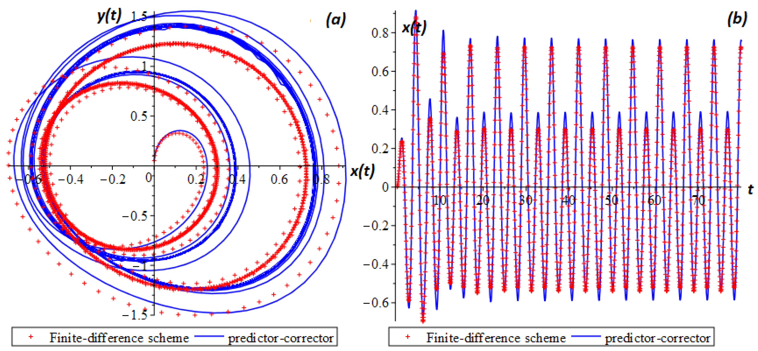
6. The Adams–Bashford–Moulton Method

Let us consider another method for solving the Cauchy problem (7)—the Adams–Bashford–Moulton method or “predictor–corrector” [29,30]. We present problem (7) as a system under homogeneous initial conditions $x\left(0\right)=\dot{x}\left(0\right)=0$:

$$\left\{\begin{array}{c}{\partial }_{0t}^{q_1\left(t\right)}x=y,q_1\left(t\right)=q\left(t\right),\hfill \\ {\partial }_{0t}^{q_2\left(t\right)}y=z,q_2\left(t\right)=1,\hfill \\ {\partial }_{0t}^{q_3\left(t\right)}z=f(x,t)-\lambda y-{\omega }_0^{2}x,q_3\left(t\right)=1-q\left(t\right),\hfill \\ x\left(0\right)=y\left(0\right)=z\left(0\right)=0,\hfill \end{array}\right.$$

(18)

In the system (18) operators of fractional derivatives of variable orders in the sense of Gerasimov–Caputo (4), in the case of homogeneous initial conditions, according to Remarks 3 and 4, they coincide with the operator of the derivative of the variable order of Riemann–Liouville (1). The solution of the system (18) is sought in the form [22,29]

$$\begin{array}{c}\hfill \left\{\begin{array}{c}{x}_{k+1}=x_0+\frac{h^{q_{n+1}^{\left(1\right)}}}{\mathsf{\Gamma }\left(q_{n+1}^{\left(1\right)}+2\right)}\left(y_{n+1}^p+{\displaystyle \sum _{j=0}^n}{\rho }_{j,n+1}^{\left(1\right)}{y}_j\right),\hfill \\ y_{k+1}=y_0+\frac{h^{q_{n+1}^{\left(2\right)}}}{\mathsf{\Gamma }\left(q_{n+1}^{\left(2\right)}+2\right)}\left(z_{n+1}^p+{\displaystyle \sum _{j=0}^n}{\rho }_{j,n+1}^{\left(2\right)}{z}_j\right),\hfill \\ z_{k+1}=z_0+\frac{h^{q_{n+1}^{\left(3\right)}}}{\mathsf{\Gamma }\left(q_{n+1}^{\left(3\right)}+2\right)}\left(f(x_{n+1}^p,t_{n+1})-\lambda y_{n+1}^p-{\omega }_0^2{x}_{n+1}^p\right)+\hfill \\ +\frac{h^{q_{n+1}^{\left(3\right)}}}{\mathsf{\Gamma }\left(q_{n+1}^{\left(3\right)}+2\right)}{\displaystyle \sum _{j=0}^n}{\rho }_{j,n+1}^{\left(3\right)}\left(f(x_j,t_j)-\lambda y_j-{\omega }_0^2{x}_j\right),\hfill \end{array}\right.\end{array}$$

(19)

where the weighting coefficients have the form

$$\left\{\begin{array}{c}{\rho }_{0,n+1}^{\left(i\right)}=n^{q_{n+1}^{\left(i\right)}+1}-\left(n-q_{n+1}^{\left(i\right)}\right){\left(n+1\right)}^{q_{n+1}^{\left(i\right)}},\hfill \\ {\rho }_{j,n+1}^{\left(i\right)}={\left(n-j+2\right)}^{q_{n+1}^{\left(i\right)}+1}+{\left(n-j\right)}^{q_{n+1}^{\left(i\right)}+1}-2{\left(n-j+1\right)}^{q_{n+1}^{\left(i\right)}+1},\hfill \\ {\rho }_{n+1,n+1}^{\left(i\right)}=1,i=1,2,3,\hfill \end{array}\right.$$

(20)

$$\left\{\begin{array}{c}{x}_{k+1}^p=x_0+\frac{h^{q_{n+1}^{\left(1\right)}}}{\mathsf{\Gamma }\left(q_{n+1}^{\left(1\right)}+1\right)}{\displaystyle \sum _{j=0}^n}{\theta }_{j,n+1}^{\left(1\right)}{y}_j,\hfill \\ y_{k+1}^p=y_0+\frac{h^{q_{n+1}^{\left(2\right)}}}{\mathsf{\Gamma }\left(q_{n+1}^{\left(2\right)}+1\right)}{\displaystyle \sum _{j=0}^n}{\theta }_{j,n+1}^{\left(2\right)}{z}_j,\hfill \\ z_{k+1}^p=z_0+\frac{h^{q_{n+1}^{\left(3\right)}}}{\mathsf{\Gamma }\left(q_{n+1}^{\left(3\right)}+1\right)}{\displaystyle \sum _{j=0}^n}{\theta }_{j,n+1}^{\left(3\right)}\left(f(x_j,t_j)-\lambda y_j-{\omega }_0^2{x}_j\right),\hfill \\ {\theta }_{j,n+1}^{\left(i\right)}={\left(n-j+1\right)}^{q_{n+1}^{\left(i\right)}}-{\left(n-j\right)}^{q_{n+1}^{\left(i\right)}},i=1,2,3.\hfill \end{array}\right.$$

(21)

Scheme (21) is a predictor (Adams–Bashford method), scheme (19) is a corrector (Adams–Moulton method).

Theorem 4.

If ${\partial }_{0t}^{q_i\left(t\right)}{x}_i\left(\tau \right)\in C^2[0,T],(x_1\left(t\right)=x\left(t\right),x_2\left(t\right)=y\left(t\right),x_3\left(t\right)=z\left(t\right),i=1,2,3)$, then

$$max|x_i\left(t_j\right)-x_{i,j}|=O\left(h^{1+\underset{i}{min}{q}_i\left(t\right)}\right)$$

(22)

Proof. 

The proof of Theorem 4 is based on the method of mathematical induction, and it is given in [30].  □

7. Simulation Results and Some Applications

7.1. Test Examples

All calculations presented in paper were performed in the Maple computer mathematics environment.

Let us consider some examples of the operation of scheme (10). Let us consider a test example when in the model Equation (7), a nonlinear function has the form

$$f(x,t)=b{x}^3\left(t\right)-b{t}^9-{\omega }_0^2{t}^3-6t-\lambda {\displaystyle \frac{d}{dt}}\left({\displaystyle \frac{\mathsf{\Gamma }\left(4\right)t^{3-q\left(t\right)}}{\mathsf{\Gamma }(4-q(t\left)\right)}}\right).$$

As a result, we obtain the following Cauchy problem

$$\ddot{x}\left(t\right)+\lambda D_{0t}^{q\left(t\right)}x\left(\tau \right)+{\omega }_0^{2}x\left(t\right)+b{x}^3\left(t\right)-b{t}^9-{\omega }_0^2{t}^3-6t-\lambda \frac{d}{dt}\left(\frac{\mathsf{\Gamma }\left(4\right)t^{3-q\left(t\right)}}{\mathsf{\Gamma }(4-q(t\left)\right)}\right)=0,$$

(23)

$$x\left(0\right)=\dot{x}\left(0\right)=0.$$

We are looking for the exact solution of the Cauchy problem (23) in the form

$$x\left(t\right)=t^3.$$

(24)

We look for error and computational accuracy according to the Runge rule [7]

$$\epsilon =max\left(|x_N^{ex}\left[j\right]-x_N\left[j\right]|\right),j=0,\dots ,N,$$

(25)

where $x_N^{ex}\left[j\right]$ is the exact solution (23), $x_N\left[j\right]$ is the numerical solution obtained by formula (10) or formulas (19) and (21). The computational accuracy of the numerical method is determined by the formula

$$\alpha ={\displaystyle \frac{ln\left({\displaystyle \frac{|{\epsilon }_i|}{|{\epsilon }_{i+1}|}}\right)}{ln\left(2\right)}}.$$

(26)

Example 1.

Let us take the following control parameters of problem (23) $q\left(t\right)=0.5{cos}^2\left(0.3t\right)$, $h=0.03875,t\in [0,3],x\left(0\right)=\dot{x}\left(0\right)=0,\lambda h^{1-Q}+h{\omega }_0^2=0.4998$.

Note that the parameter values were chosen in such a way that the conditions of Theorems 2 and 3 were fulfilled. The calculated curves obtained by formula (24) and numerical scheme (10) for $N=80$ are shown in Figure 1.

It can be seen from Figure 1 that when the conditions of Theorems 2 and 3 are met, the numerical scheme (10) approximates the exact solution (24) well. This result also confirms the calculation of computational accuracy (26) according to

Table 1. Error and computational accuracy of the numerical scheme (10).

N	h	$\mathit{\epsilon }$ (25)	$\mathit{\alpha }$ (26)
10	0.1	0.010416664	-
20	0.05	0.005137254	1.019824008
40	0.025	0.002556096	1.007055385
80	0.0125	0.001275018	1.003424407
160	0.00625	0.000636774	1.001664279
320	0.003125	0.000318209	1.00080679
640	0.0015625	0.000159059	1.000412635

.

From Table 1 we see that when the nodes of the calculated grid are doubled, the error (25) decreases also by about two times. At the same time, computational accuracy tends to unity, which does not contradict Remark 9.

Let us take other parameter values at which the conditions of Theorems 2 and 3 are violated.

Example 2.

Let us take the following control parameters $q\left(t\right)=0.5{cos}^2\left(0.3t\right),h=0.041375,$ $t\in [0.3,3.32],x\left(0\right)=\dot{x}\left(0\right)=0,\lambda h^{1-Q}+h{\omega }_0^2=0.5084$.

The simulation results are shown in Figure 2.

Here, we see that with a slight increase in the simulation time compared to Example 1, there is a discrepancy between the values obtained by formula (24) and the explicit finite difference scheme (10). We can also observe a violation of the stability of the numerical scheme (10) by changes in the value of the computational accuracy $\alpha$ in

Table 2. Error and computational accuracy of the numerical scheme (10).

N	h	$\mathit{\epsilon }$ (18)	$\mathit{\alpha }$ (19)
10	0.1	216.8838	-
20	0.05	11004.94	−5.665085173
40	0.025	22.6488	8.92450095
80	0.0125	0.012252099	10.85218997
160	0.00625	0.006278409	0.96455801
320	0.003125	0.0031782	0.9821891
640	0.0015625	0.0015990701	0.990976729

.

Example 3.

Let us take the following control parameters for problem (23) $t\in [0,1],h=0.05,$ $x\left(0\right)=\dot{x}\left(0\right)=0,\lambda =1,{\omega }_0=b=\delta =omega=1,q\left(t\right)=0.5{cos}^2\left(0.2t\right)$.

Figure 3 shows the curve of the numerical solution obtained by schemes (10) and (19) for test example 3. According to Figure 3 and

Table 3. Error and computational accuracy of the numerical scheme (10) and “predictor–corrector” method.

N	h = T/N	$\mathit{ϵ}$ (Finite-Difference Scheme (10))	$\mathit{\alpha }$ (Finite-Difference Scheme (10))	$\mathit{ϵ}$ (Predictor–Corrector (19))	$\mathit{\alpha }$ (Predictor–Corrector (19))
10	0.1	0.010416664	-	0.022014375	-
20	0.05	0.005137254	1.019824008	0.006517327	0.758163925
40	0.025	0.002556096	1.007055385	0.002125805	0.817941863
80	0.0125	0.001275018	1.003424407	0.004337276	1.131071553
160	0.00625	0.000636774	1.001664279	0.005145645	1.03243208
320	0.003125	0.000318209	1.00080679	0.005452087	1.011099493
640	0.0015625	0.000159059	1.000412635	0.005571391	1.004170658

, schemes (10) and (19) converge to the exact solution with a decrease in the iteration step. By Theorem 4, the predictor–corrector scheme (19) converges with the order $O\left(h^{1+\underset{i}{min}{q}_i\left(t\right)}\right)$, and since in example 3 the order of the derivative is represented as a function $q\left(t\right)=0.5cos\left(0.2t\right)$, the minimum of which is 1, then in the end, for our example, the predictor–corrector has the first order of accuracy. According to Table 3, the computational accuracy tends to 1.

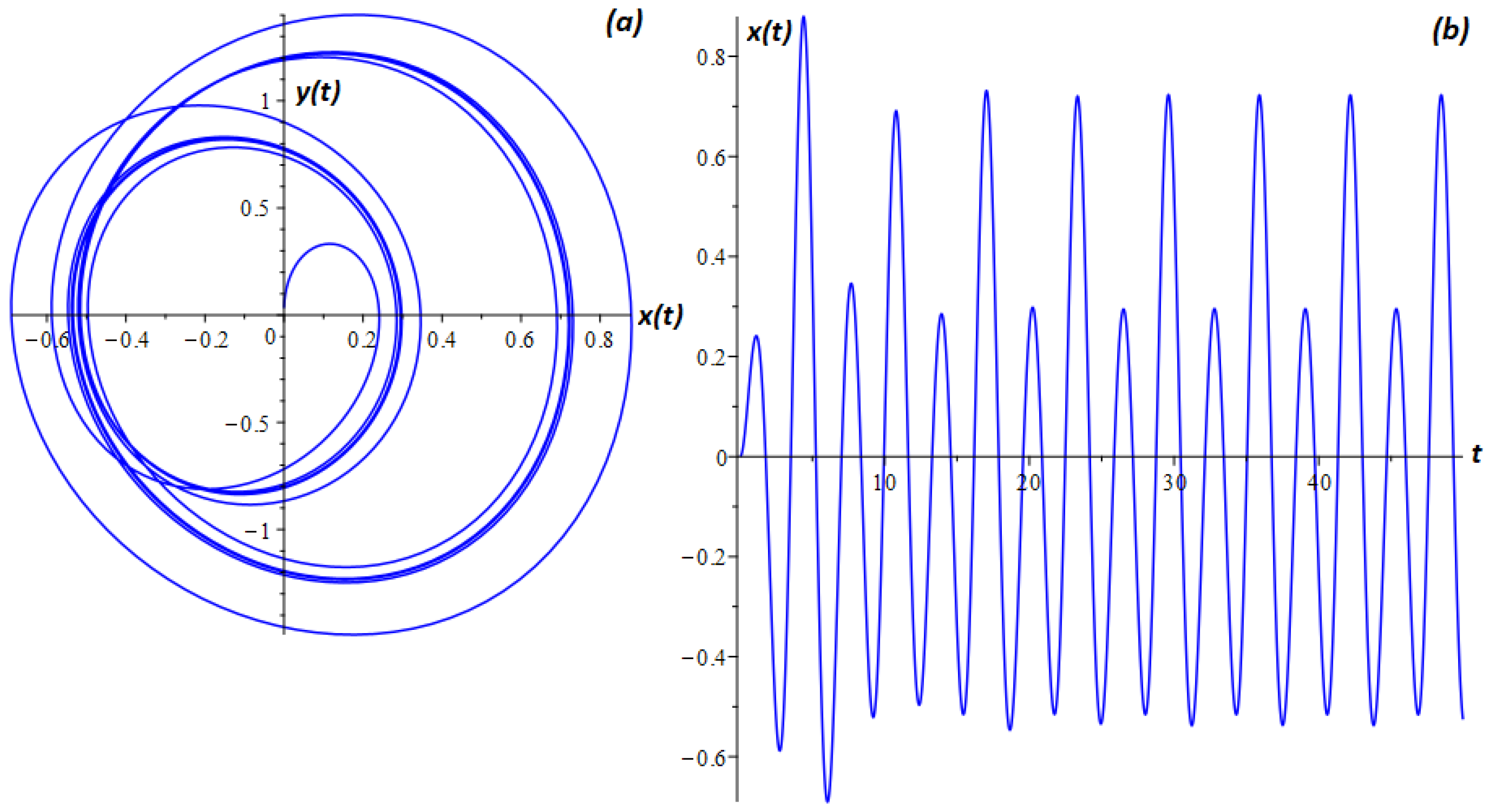
7.2. Fractional Duffing Oscillator

Let us consider a fractional Duffing oscillator with external influence, when in the model of Equation (7), the function of external influence $f\left(x,t\right)=b{x}^3\left(t\right)-\delta cos\left(\omega t\right)$, $\delta$ and $\omega$ are the amplitude and frequency of external influence, and b is the coefficient responsible for the non-isochronicity of oscillations, i.e., the dependence of their period on the amplitude.

As a result, we obtain the model equation

$$\ddot{x}\left(t\right)+\lambda D_{0t}^{q\left(t\right)}x\left(t\right)+{\omega }_0^{2}x\left(t\right)+b{x}^3\left(t\right)=\delta cos\left(\omega t\right),$$

(27)

The fractional Duffing oscillator (27) has various applications, for example, it is used as a model for describing a tsunami [31] or for constructing a PID controller [32].

Example 4.

The values of the parameters in the model Equation (27) are chosen as follows: $q\left(t\right)=0.8{cos}^2\left(0.5t\right),h=0.0575,t\in [0,50],x\left(0\right)=\dot{x}\left(0\right)=0,\lambda ={\omega }_0=b=\delta =1,\omega =1.8$.

The waveform and phase trajectory ($y\left(t\right)=\dot{x}\left(t\right)$) obtained using the explicit finite difference scheme (10) are shown in Figure 4.

The Duffing oscillator has various oscillatory regular and chaotic modes. Regular modes can be many periodic. Figure 4 shows an example of two periodic modes when there are fluctuations with several periods. The oscillogram in Figure 4b shows that over time, the oscillations reach a steady two-period mode, and the phase trajectory Figure 4a has the form of a closed loop, which characterizes several periods of oscillation.

Note that the values of the parameters in the model Equation (27) were chosen so that the conditions for the fulfillment of Theorems 2 and 3 are satisfied. We estimate the computational accuracy using the double recalculation method. To do this, we look for the error of the numerical method using the formula

$$\epsilon =max\left(|x_{2j}-x_j|\right),j=0,\dots ,N,$$

(28)

where $x_{2j}$ is the numerical solution at the step $\frac{h}{2}$, $x_j$ is the numerical solution at step h obtained by formula (10). The computational accuracy of the method is determined by formula (28). The simulation results are shown in Table 3.

From

Table 4. Error and computational accuracy of scheme (10).

N	h	$\mathit{\epsilon }$ (28)	$\mathit{\alpha }$ (16)
10	0.1	0.010416664	-
20	0.05	0.005137254	1.019824008
40	0.025	0.002556096	1.007055385
80	0.0125	0.001275018	1.003424407
160	0.00625	0.000636774	1.001664279
320	0.003125	0.000318209	1.00080679
640	0.0015625	0.000159059	1.000412635

, we see that increasing the nodes of the computational grid by a factor of 2 leads to a reduction in the error by a factor of 2, while the computational accuracy of the method tends to unity $\alpha \to 1$. The latter fact does not contradict Remark 9.

Consider the computational accuracy of the method in a situation where the conditions of Theorems 2 and 3 are violated. To do this, select the values of the parameters $t\in [0,80],$$h=0.0533,\lambda h^{1-Q}+h{\omega }_0^2=0.5297$, and leave the other parameters unchanged. The results of calculating the computational accuracy of the numerical method (10) are given in

Table 5. Error and computational accuracy of the scheme (10).

N	h	$\mathit{\epsilon }$ (20)	$\mathit{\alpha }$ (19)
10	0.1	0.010416664	-
20	0.05	0.055137254	−2.404134099
40	0.025	0.006556096	3.072118534
80	0.0125	0.003275018	1.001334144
160	0.00625	0.001536774	1.09159782
320	0.003125	0.00078209	0.974498474
640	0.0015625	0.000039059	1.001679624

.

From Table 5, we can see that the computational accuracy of the method has a pronounced non-monotonic character in changing its values, which confirms the violation of the stability and convergence of the method (10). However, in this example, an increase in the nodes of the computational grid N by two times also leads to a reduction in the error by about two times.

Example 5.

The values of the parameters in the model Equation (27) are chosen as follows: $t\in [0,100],$$h=0.05,x\left(0\right)=\dot{x}\left(0\right)=0,\lambda =1,{\omega }_0=b=\delta =omega=1,$$q\left(t\right)=0.5{cos}^2\left(0.2t\right)$.

As can be seen from

Table 6. Error and computational accuracy of the numerical scheme (10) and “predictor–corrector” method.

N	$\mathit{h}=\mathit{T}/\mathit{N}$	$\mathit{ϵ}$ (Finite-Difference Scheme (10))	$\mathit{\alpha }$ (Finite-Difference Scheme (10))	$\mathit{ϵ}$ (Predictor–Corrector (19))	$\mathit{\alpha }$ (Predictor–Corrector (19))
10	0.1	0.010416664	-	0.012159916	-
20	0.05	0.005137254	1.019824008	0.005933937	1.035071832
40	0.025	0.002556096	1.007055385	0.002947911	1.009296592
80	0.0125	0.001275018	1.003424407	0.001468966	1.004891965
160	0.00625	0.000636774	1.001664279	0.000733796	1.001351042
320	0.003125	0.000318209	1.00080679	0.000366708	1.000745531
640	0.0015625	0.000159059	1.000412635	0.00018197	1.000434281

, there is no difference between the explicit finite difference scheme (10) and the predictor-corrector scheme (19). Both schemes have practically the same convergence rate. Their computational accuracy tends to 1.

Let us consider the operation of an explicit finite-difference scheme (10) for calculating an important characteristic of an oscillatory system—the amplitude–frequency characteristic.

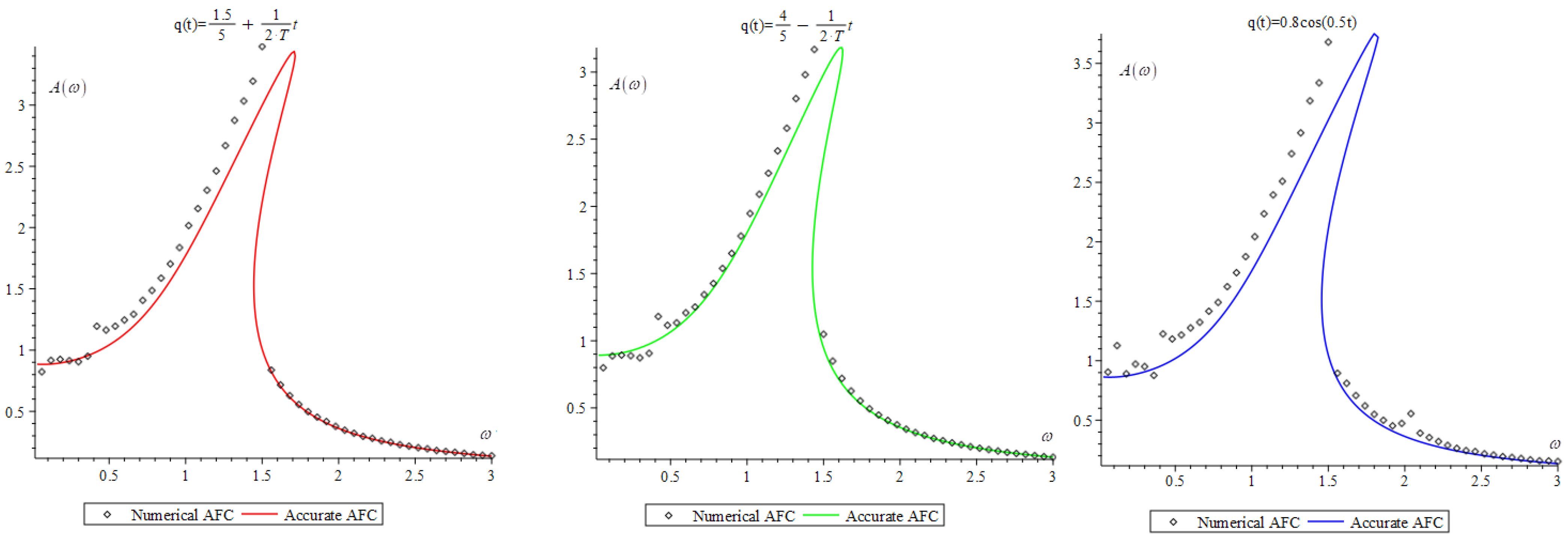
7.3. Amplitude–Frequency Characteristic of a Fractional Duffing oscillator

The amplitude–frequency characteristic is the dependence of the amplitude of steady-state oscillations of the output signal of a certain system on the frequency of its input harmonic signal.

In [22,33], a formula was obtained for calculating the amplitude–frequency characteristic of a fractional Duffing oscillator with a Riemann–Liouville derivative of fractional variable order. The Cauchy problem (27) can be represented as a linear equation, which we obtain by substituting in (27) the solution in the form of the first harmonic [22] $x\left(t\right)=Acos(\omega t+\varphi )$.

$$\ddot{x}\left(t\right)+p\dot{x}\left(t\right)+s^{2}x\left(t\right)=\delta cos\left(\omega t\right),$$

(29)

$$p=-2\lambda {\omega }^{q\left(t\right)-1}sin\left(\frac{q\left(t\right)\pi }{2}\right)+$$

$$2\lambda \frac{dq}{dt}{\omega }^{q\left(t\right)-2}\left[(ln\left(\omega \right)-\mathsf{\Psi }(1-q\left(t\right)))cos\left(\frac{q\left(t\right)\pi }{2}\right)+\frac{\pi sin\left(\frac{q\left(t\right)\pi }{2}\right)}{2}\right],$$

(30)

$$s^2={\omega }_0^2-2\lambda {\omega }^{q\left(t\right)}cos\left(\frac{q\left(t\right)\pi }{2}\right)+\frac{3A^{2}b}{4}-$$

(31)

$$2\lambda \frac{dq}{dt}{\omega }^{q\left(t\right)-1}\left[(ln\left(\omega \right)-\mathsf{\Psi }(1-q\left(t\right)))sin\left(\frac{q\left(t\right)\pi }{2}\right)+\frac{\pi cos\left(\frac{q\left(t\right)\pi }{2}\right)}{2}\right].$$

Equation (29) is the equation of a classical linear oscillator, for which the formula for the amplitude–frequency response is known.

$$A\left(\omega \right)=\frac{\delta }{\sqrt{{(s^2-{\omega }^2)}^2+p^2{\omega }^2}},$$

(32)

In (30) and (31) $\mathsf{\Psi }(1-q\left(t\right))=-\gamma +{\displaystyle \sum _{n=1}^{\infty }}\left({\displaystyle \frac{1}{n}}-{\displaystyle \frac{1}{n+1-q\left(t\right)}}\right)$ is the digamma function, where $\gamma =\frac{1}{2}(\sqrt[3]{10}-1)$ is Euler’s constant. In practice, it is enough to take $n=50$.

To calculate the amplitude–frequency characteristic, we use an explicit Euler’s method (10), and then compare the results obtained with the results of calculations using the analytical formula (32). To do this, we carry out the calculation according to scheme (10) with a sufficiently long simulation time, in which the forced oscillations reach a steady state. Next, the amplitude values are fixed at different values of the frequency of external influence, and we obtain the dependence $A\left(\omega \right)$, which is plotted by points.

Figure 5 shows the simulation results for various types of the function $q\left(t\right)$, which have monotone and non-monotone properties. The values of the calculated parameters are as follows: $t\in [0,100],h=0.05,x\left(0\right)=\dot{x}\left(0\right)=0,\lambda =0.1,{\omega }_0=b=\delta =1$, and the frequency of external action $\omega \in [0,3]$ is changed in increments of $h_{\omega }=0.6$.

From Figure 5, we see that the explicit finite-difference scheme approximates the amplitude–frequency characteristic obtained by the analytical formula (32) quite well when the $q\left(t\right)$ order of the fractional Riemann–Liouville derivative is a monotone function. In the case when $q\left(t\right)$ is nonmonotonic, then the approximation according to the explicit finite difference scheme (10) can be considered satisfactory in some approximation. In this case, the accuracy of calculations can be improved by constructing implicit finite difference schemes with higher accuracy.

It should be noted that the curves in Figure 6 are called resonant curves, and the resonant frequency ${\omega }_R$ can be determined from ${\displaystyle \frac{dA\left({\omega }_R\right)}{d{\omega }_R}}=0$ as the maximum of the function. It was shown in [3,4,5,6] that the resonant frequency can shift to regions of lower or higher frequencies depending on the order of the fractional derivative, i.e., in fact, a connection was established between the order of the fractional derivative and the Q-factor of the oscillatory system [34].

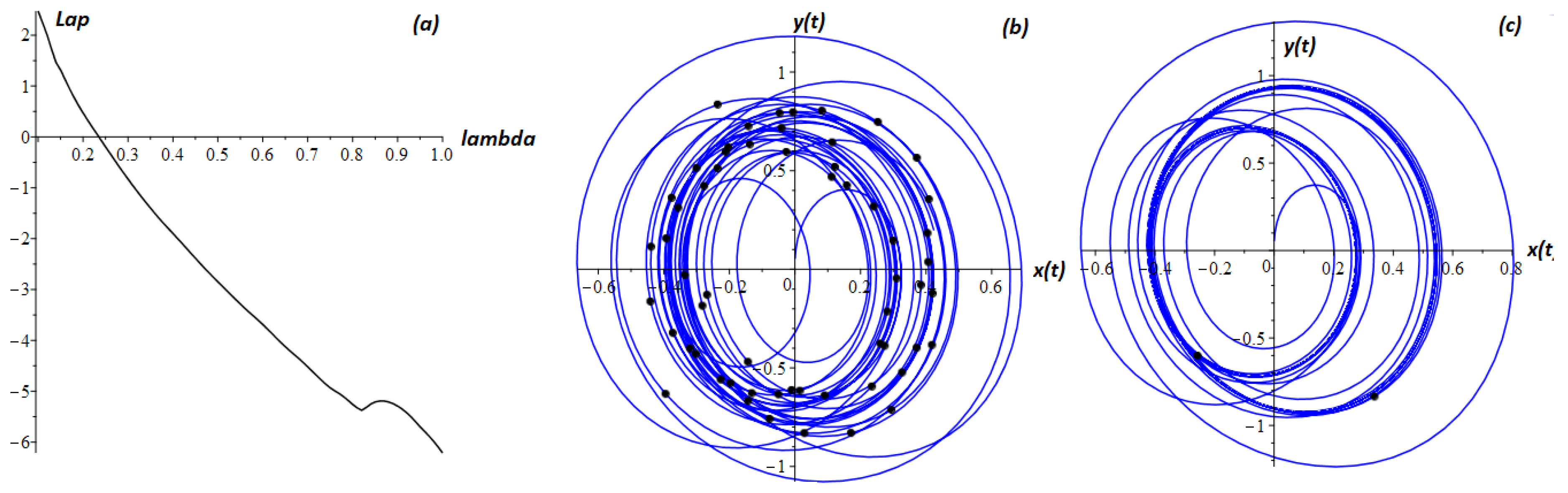
8. The Study of Chaotic and Regular Modes

In the study of nonlinear systems, one of the important tasks is to determine the type of oscillations—periodic, quasi-periodic, random, and chaotic. It is especially difficult to distinguish quasiperiodic oscillations from chaotic and random ones, since quasiperiodic oscillations often have a very complex shape that is visually indistinguishable from “random” ones [11].

A feature of chaotic oscillations is their high sensitivity to small changes in initial conditions. Therefore, one of the most reliable ways to detect chaos is to determine the speed of the trajectory run-up, which is estimated using a spectrum of Lyapunov exponents [35].

Consider the Wolf–Benettin algorithm [22,35] for calculating Lyapunov exponents. We present problem (7) as a system:

$$\left\{\begin{array}{c}\dot{x}\left(t\right)=y\left(t\right)\hfill \\ \dot{y}\left(t\right)=f(x,t)-\lambda D_{0t}^{q\left(t\right)}x\left(t\right)-{\omega }_0^{2}x\left(t\right)\hfill \\ x\left(0\right)=y\left(0\right)=0.\hfill \end{array}\right.$$

(33)

If two trajectories remain close over time, then their change obeys the law

$$u_{j+1}=J\left(u_j\right)u_j,J\left(u_j\right)=\left(\begin{array}{cc}\frac{\partial f_1}{\partial x_j}& \frac{\partial f_1}{\partial y_j}\\ \frac{\partial f_2}{\partial x_j}& \frac{\partial f_2}{\partial y_j}\end{array}\right),$$

(34)

where $J\left(u_j\right)$ is the Jacobi matrix, and $f_1$ and $f_2$ are the right parts of system (33). With the help of system (34), variational equations are compiled.

The Wolf–Benettin algorithm [35]:

1. Select the starting point of the vector $x_0$ and together with it, we will track the K disturbed trajectories. Let $K=2$.

2. We solve the system (33) numerically, using scheme (10), with two sets of perturbed Equation (34). As the initial vectors for equations in variations, you must select a set of vectors $\widehat{x_0^0},\widehat{y_0^0}$ that are orthogonal and normalized by one. We are looking for numerical solutions of systems in the form:

$$\left\{\begin{array}{c}{x}_k=h{y}_{k-1}+x_{k-1}\hfill \\ y_k=y_{k-1}+h(f(x_{k-1},t_{k-1})-\lambda h^{-q_k}{\displaystyle \sum _{i=0}^{k-1}}{c}_i^{q_k}{x}_{k-i}-{\omega }_0^2{x}_{k-1})\hfill \end{array}\right.$$

(35)

$$\left\{\begin{array}{c}x{x}_k=hy{y}_{k-1}+x{x}_{k-1}\hfill \\ y{y}_k=y{y}_{k-1}+h(({\omega }_0^2-f_{x{x}_{k-1}}^{\prime }(x{x}_{k-1},t_{k-1}))x{x}_{k-1}-\lambda h^{-q_k}{\displaystyle \sum _{i=0}^{k-1}}{c}_i^{q_k}x{x}_{k-i})\hfill \\ x{x}_0=1,y{y}_0=0\hfill \end{array}\right.$$

(36)

$$\left\{\begin{array}{c}X{X}_k=hY{Y}_{k-1}+X{X}_{k-1}\hfill \\ Y{Y}_k=Y{Y}_{k-1}+h(({\omega }_0^2-f_{X{X}_{k-1}}^{\prime }(X{X}_{k-1},t_{k-1}))X{X}_{k-1}-\lambda h^{-q_k}{\displaystyle \sum _{i=0}^{k-1}}{c}_i^{q_k}X{X}_{k-i})\hfill \\ X{X}_0=0,Y{Y}_0=1\hfill \end{array}\right.$$

(37)

The scheme (35) is a numerical solution of the system (33). The numerical solutions of Schemes (36) and (37) of perturbed Equation (35), where $x{x}_k$ and $y{y}_k$ are coordinates of perturbation vectors under initial conditions $x{x}_0=1$, $y{y}_0=0$, $X{X}_k$ and $Y{Y}_k$, are the coordinates of the perturbation vectors under initial conditions $X{X}_0=0$, $Y{Y}_0=1$.

3. After time T, the trajectory moves to the point vector $x_1$, the perturbation vectors $\widehat{x_1},\widehat{y_1}$, which we renormalize using the Gram–Schmidt method.

$$\widehat{x_1^0}=\frac{\widehat{x_1}}{\parallel \widehat{x_1}\parallel },$$

$$\widehat{y_1^{\prime }}=\widehat{y_1}-(\widehat{y_1},\widehat{x_1^0})\widehat{x_1^0},\widehat{y_1^0}=\frac{\widehat{y_1^{\prime }}}{\parallel \widehat{y_1^{\prime }}\parallel }$$

Steps 1–3 are repeated M times, and the sums of the calculations are calculated: $S_1={\displaystyle \sum _{i=1}^M}ln(\parallel \widehat{x_i}\parallel )$, $S_2={\displaystyle \sum _{i=1}^M}ln(\parallel \widehat{y_i}\parallel )$. The estimation of Lyapunov exponents is calculated using the formula:

$${\mathsf{\Lambda }}_i=\frac{S_i}{MT},i=1,2.$$

Example 6.

The values of the parameters in system (33) are chosen as follows: $q\left(t\right)=0.8{cos}^2\left(0.5t\right),$$f\left(x,t\right)=b{x}^3\left(t\right)-\delta cos\left(\omega t\right),h=0.025,t\in [0,50],x\left(0\right)=\dot{x}\left(0\right)=0,$${\omega }_0=b=\omega =1,\delta =1$.

Figure 7 shows the spectrum of Lyapunov exponents relative to the coefficient of dissipation $\lambda$. The figures show that with positive values of the spectrum of Lyapunov exponents, a chaotic regime is observed, and with negative values, a regular one.

Example 7.

The values of the parameters in system (33) are chosen as follows: $f\left(x,t\right)=b{x}^3\left(t\right)-\delta cos\left(\omega t\right),h=0.025,t\in [0,50],x\left(0\right)=\dot{x}\left(0\right)=0,\lambda ={\omega }_0=b=\omega =1,\delta =1$.

In Figure 7 and Figure 8, Poincaré sections are indicated by points on the phase trajectories. The number of Poincaré sections corresponds to the number of oscillation periods.

9. Conclusions

In this paper, we proposed a simple non-local explicit finite-difference scheme based on the discrete Grunwald–Letnikov derivative for the numerical solution of the Cauchy problem (7). In this paper, we considered the issues of stability and convergence of the proposed scheme. For the first time, the stability and convergence theorem of an explicit Euler’s method was proved. We showed that the non-local finite-difference scheme is conditionally stable and converges with the first order. We reviewed test cases, gave an assessment of the computational accuracy, which is consistent with theoretical calculations. Examples of the calculation of oscillograms, phase trajectories and frequency response of a fractional Duffing oscillator were considered. We showed the acceptability of a non-local explicit finite-difference scheme for numerical analysis of a fractional Duffing oscillator.

The results obtained in the work can be improved by developing non-local implicit finite-difference schemes with higher accuracy. This is the next stage of research development that the authors intend to implement. It should be noted that the fractional Duffing oscillator has rich dynamics, various modes and effects. For example, it is known that the fractional Duffing oscillator has a bistable behavior—a jump or dynamic hysteresis. This can be seen, for example, in Figure 4. for the frequency response, plotted by points. Therefore, it makes sense to investigate the bistable behavior depending on the order of the fractional derivative as a function of time, by analogy with the work [36].

In the future, it is planned to study the case when the fractional derivative of a variable order depends not only on time t, but also on the solution function $x\left(t\right)$ by analogy with the works [25,26].

References

1. Petras, I. Fractional-Order Nonlinear Systems: Modeling, Analysis and Simulation; Springer: New York, NY, USA, 2010; p. 180. [Google Scholar]
2. Shitikova, M.V. Fractional Operator Viscoelastic Models in Dynamic Problems of Mechanics of Solids: A Review. Mech. Solids 2021, 57, 1–33. [Google Scholar] [CrossRef]
3. Rekhviashvili, S.S.; Pskhu, A.V. New method for describing damped vibrations of a beam with a built-in end. Tech. Phys. 2019, 64, 1237–1241. [Google Scholar] [CrossRef]
4. Parovik, R.I. Quality factor of forced oscillations of a linear fractional oscillator. Tech. Phys. 2020, 65, 1059–1063. [Google Scholar] [CrossRef]
5. Parovik, R.I. Amplitude-frequency and phase-frequency performances of forced oscillations of a nonlinear fractional oscillator. Tech. Phys. Lett. 2019, 45, 660–663. [Google Scholar] [CrossRef]
6. Rekhviashvili, S.S.; Pskhu, A.V. Fractional oscillator with exponential power function of memory. Lett. ZhTF 2022, 48, 33–35. (In Russian) [Google Scholar]
7. Syta, A.; Litak, G.; Lenci, S.; Scheffler, M. Chaotic vibrations of the Duffing system with fractional damping. Chaos Interdiscip. J. Nonlinear Sci. 2014, 24, 10–16. [Google Scholar] [CrossRef]
8. Xu, Y.; Li, Y.; Liu, D.; Jia, W.; Huang, H. Responses of Duffing oscillator with fractional damping and random phase. Nonlinear Dyn. 2013, 74, 745–753. [Google Scholar] [CrossRef]
9. Shen, Y.; Li, H.; Yang, S.; Peng, M.; Han, Y. Primary and subharmonic simultaneous resonance of fractional-order Duffing oscillator. Nonlinear Dyn. 2020, 102, 1485–1497. [Google Scholar] [CrossRef]
10. Xing, W. Threshold for chaos of a duffing oscillator with fractional-order derivative. Shock Vib. 2019, 2019, 1–16. [Google Scholar] [CrossRef]
11. Gao, X. Chaos in the fractional order periodically forced complex Duffing’s oscillators. Chaos Solitons Fractals 2005, 24, 97–104. [Google Scholar] [CrossRef]
12. El-Dib, Y.O. Stability approach of a fractional-delayed Duffing oscillator. Discontinuity Nonlinearity Complex 2020, 9, 367–376. [Google Scholar] [CrossRef]
13. Eze, S.C. Analysis of fractional Duffing oscillator. Rev. Mex. Física 2020, 66, 187–191. [Google Scholar] [CrossRef]
14. Gouari, Y.; Dahmani, Z.; Jebril, I. Application of fractional calculus on a new differential problem of duffing type. Adv. Math. Sci. J. 2020, 9, 10989–11002. [Google Scholar] [CrossRef]
15. Barba-Franco, J.J.; Gallegos, A.; Jaimes-Reátegui, R.; Pisarchik, A.N. Dynamics of a ring of three fractional-order Duffing oscillators. Chaos Solitons Fractals 2022, 155, 111–747. [Google Scholar] [CrossRef]
16. Ejikeme, C.L.; Oyesanya, M.O.; Agbebaku, D.F.; Okofu, M.B. Solution to nonlinear Duffing oscillator with fractional derivatives using homotopy analysis method (HAM). Glob. J. Pure Appl. Math. 2018, 14, 1363–1388. [Google Scholar]
17. Syam, M.I. The Modified Fractional Power Series Method for Solving Fractional Undamped Duffing Equation with Cubic Nonlinearity. Nonlinear Dyn. Syst. Theory 2020, 20, 568–577. [Google Scholar]
18. Alvaro, H.; Salas, S. Analytical Approximant to a Quadratically Damped Duffing Oscillator. Sci. World J. 2022, 2022, 10–21. [Google Scholar]
19. Wawrzynski, W. The origin point of the unstable solution area of a forced softening Duffing oscillator. Sci. Rep. 2022, 12, 4518. [Google Scholar] [CrossRef]
20. Chen, T.; Cao, X.; Niu, D. Model modification and feature study of Duffing oscillator. J. Low Freq. Noise 2022, 41, 230–243. [Google Scholar] [CrossRef]
21. Kim, V.A. Duffing oscillator with an external harmonic impact and derived variables fractional Remann-Liouville, is characterized by viscous friction. Bulletin KRASEC. Phys. Math. Sci. 2016, 13, 46–49. [Google Scholar]
22. Kim, V.A.; Parovik, R.I. Mathematical model of fractional Duffing oscillator with variable memory. Mathematics 2020, 8, 2063. [Google Scholar] [CrossRef]
23. Nakhushev, A.M. Fractional Calculus and Its Applications; Fizmatlit: Moscow, Russia, 2003; p. 272. (In Russian) [Google Scholar]
24. Kilbas, A.A.; Srivastava, H.M.; Trujillo, J.J. Theory and Applications of Fractional Differential Equations; Elsevier Science Limited: Amsterdam, The Netherlands, 2006; Volume 204, p. 523. [Google Scholar]
25. Zhuang, P.; Liu, F.; Anh, V.; Turner, I. Numerical methods for the variable-order fractional advection-diffusion equation with a nonlinear source term. SIAM J. Numer. Anal. 2009, 47, 1760–1781. [Google Scholar] [CrossRef] [Green Version]
26. Sun, H.; Chang, A.; Zhang, Y.; Chen, W. Variable-order fractional differential equations: Mathematical foundations, physical models, numerical methods and applications. Fract. Calc. Appl. Anal. 2019, 22, 27–59. [Google Scholar] [CrossRef] [Green Version]
27. Nigmatullin, R.R. Fractional integral and its physical interpretation. Theor. Math. Phys. 1992, 90, 242–251. [Google Scholar] [CrossRef]
28. Meerschaert, M.M.; Tadjeran, C. Finite difference approximations for fractional advection–dispersion flow equations. J. Comput. Appl. Math. 2004, 172, 65–77. [Google Scholar] [CrossRef] [Green Version]
29. Parovik, R.I. Mathematical modeling of linear fractional oscillators. Mathematics 2020, 8, 1879. [Google Scholar] [CrossRef]
30. Yang, C.; Liu, F. A computationally effective predictor-corrector method for simulating fractional-order dynamical control system. ANZIAM J. 2006, 47, 168–184. [Google Scholar] [CrossRef] [Green Version]
31. Niu, J.; Shen, Y.; Yang, S.; Li, S. Analysis of Duffing oscillator with time-delayed fractional-order PID controller. Int. J. Non-Linear Mech. 2017, 92, 65–75. [Google Scholar] [CrossRef]
32. Wang, Y.; An, J.Y. Amplitude–frequency relationship to a fractional Duffing oscillator arising in microphysics and tsunami motion. J. Low Freq. Noise Vib. Act. Control 2019, 38, 1008–1012. [Google Scholar] [CrossRef]
33. Li, Y.; Duan, J.-S. The periodic response of a fractional oscillator with a spring-pot and an inerter-pot. J. Mech. 2020, 37, 108–117. [Google Scholar] [CrossRef]
34. Yang, J.H.; Sanjuán, M.A.; Wang, C.J.; Zhu, H. Vibrational Resonance in a Duffing System with a Generalized Delayed Feedback. J. Appl. Nonlinear Dyn. 2013, 2, 397–408. [Google Scholar] [CrossRef]
35. Wolf, A.; Swift, J.B.; Swinney, H.L.; Vastano, J.A. Determining Lyapunov exponents from a time series. Phys. Nonlinear Phenom. 1985, 16, 285–317. [Google Scholar] [CrossRef] [Green Version]
36. Parovik, R.I. Dynamic hysteresis of a fractional Duffing oscillator. Mat. Instituti Byulleteni 2019, 6, 47–51. (In Russian) [Google Scholar]
Figure 1. Test example. Numerical and exact solutions of problem (23) in case of fulfillment of the condition of Theorems 2 and 3.
Fractalfract 06 00274 g001
Figure 2. Test example. Numerical and exact solutions of problem (20) when the conditions of Theorems 2 and 3 are not fulfilled.
Fractalfract 06 00274 g002
Figure 3. A test example. Solutions of the Cauchy problem (7) obtained by schemes (10), (19) and (21), as well as the exact solution (24).
Fractalfract 06 00274 g003
Figure 4. Phase trajectory (a) and oscillogram (b) for the Cauchy problem (1) under the conditions of Theorems 2 and 3 at N = 1500 .
Fractalfract 06 00274 g004
Figure 5. Amplitude–frequency characteristic of the fractional Duffing oscillator for various types of the q ( t ) function.
Fractalfract 06 00274 g005
Figure 6. Phase trajectory (a) and waveforms (b) obtained from schemes (10) and (19).
Fractalfract 06 00274 g006
Figure 7. The spectrum of Lyapunov exponents from λ (a) and phase trajectories at (b) λ = 0.18 , (c) λ = 0.6 . The dots represent the Poincaré sections.
Fractalfract 06 00274 g007
Figure 8. The spectrum of Lyapunov exponents from q ( t ) (a) and phase trajectories at (b) q ( t ) = 0.15 cos 2 ( 0.2 t ) , (c) q ( t ) = 0.8 cos 2 ( 0.5 t ) . The dots represent the Poincaré sections.
Fractalfract 06 00274 g008