Article

New Solutions of Nonlinear Dispersive Equation in Higher-Dimensional Space with Three Types of Local Derivatives

1
Department of Mathematics, Art and Science Faculty, Siirt University, Siirt 56100, Turkey
2
Department of Mathematics, Basic Science Faculty, University of Bonab, Bonab P.O. Box 55513-95133, Iran
3
Department of Mathematics, Çankaya University, Ankara 06790, Turkey
4
Department of Mathematics, King Abdulaziz University, P.O. Box 80257, Jeddah 21589, Saudi Arabia
5
Department of Medical Research, China Medical University, China Medical University, Taichung 40402, Taiwan
*
Authors to whom correspondence should be addressed.
Fractal Fract. 2022, 6(4), 202; https://doi.org/10.3390/fractalfract6040202
Submission received: 28 February 2022 / Revised: 22 March 2022 / Accepted: 31 March 2022 / Published: 4 April 2022

Abstract

:
The aim of this paper is to use the Nucci’s reduction method to obtain some novel exact solutions to the s-dimensional generalized nonlinear dispersive mK(m,n) equation. To the best of the authors’ knowledge, this paper is the first work on the study of differential equations with local derivatives using the reduction technique. This higher-dimensional equation is considered with three types of local derivatives in the temporal sense. Different types of exact solutions in five cases are reported. Furthermore, with the help of the Maple package, the solutions found in this study are verified. Finally, several interesting 3D, 2D and density plots are demonstrated to visualize the nonlinear wave structures more efficiently.

1. Introduction

Nonlinear partial differential equations (NPDEs) play a significant role in almost all branches of science and technology [1,2,3,4,5,6]. Solutions to these problems can describe many natural phenomena in engineering, chemistry, physics, etc. Therefore, exact solutions to Nonlinear partial differential equations is an interesting field for many researchers and there are various types of methods to find exact solutions to these problems. Additionally, there are some studies about the practical investigation of natural models. For example, in [7], significant chaotic features for different experimental conditions that are useful for the initial understanding of two-phase flow patterns in complex micro-channels, are considered. An optical system is presented to provide an innovative solution for distributed detection in microfluidics as a bridge between point-wise and full-field off-line monitoring systems [8].
Many studies have been carried out in recent years to find new solutions to these equations, using various techniques. For example, the Lie symmetry method [9,10,11,12], invariant subspace method [13,14,15], the exponential rational function method [16,17,18], the modified simple equation method [19,20,21], the Exp function method [22,23], the modified extended tanh-function method [24,25], and the Kudryashov method [26,27]. Different types of exact solutions are reported using these approaches. Among them, soliton-type solutions play an important role in science and engineering. N-soliton solutions for the coupling of differential equations and higher-dimensional differential equations are investigated in the literature [28,29,30,31,32,33,34,34].
One of the interesting NPDEs, which was first reported by Rosenau and Hyman [35], is the K(m,n) equation:
u t + ( u m ) x + ( u n ) x x x = 0 , m > 0 , 1 < n 3 .
Indeed, this equation is the Korteweg–de Vries-like equation with nonlinear dispersion. The role of nonlinear dispersion in the formation of patterns in liquid drops (nuclear physics) is interpreted by the aforementioned K(m,n) equation. The very closed behavior and stability of solitary waves with compact support (compactons) to completely integrable systems were found.
A natural generalization of the K(m,n) equation is the generalized nonlinear dispersive mK(m,n) equations in a higher dimension [36,37]:
u n 1 u t + a ( u m ) x + i = 1 s α i ( u n ) x i x i x i = 0 , n 1 ,
where α i are constants. In [38], the bifurcation behavior of travelling wave solutions of Equation (2) by s = 1 , along with all possible exact explicit parametric representations for periodic travelling wave solutions, solitary wave solutions, kink and anti-kink wave solutions and periodic cusp wave solutions are investigated. Moreover, a new version of Equation (2), that is, the modified K(m,n,k), is discussed in [39]. Some compacton solutions and solitary pattern solutions of mK(m,n, k) equations are reported in this paper.
In this work, we investigate analytical solutions to the s dimensional mK(m,n) equation with a recently defined local derivative [40]:
u n 1 D t u + a ( u m ) x + i = 1 s α i ( u n ) x i x i x i = 0 , a , α i R ,
where the operator D t { 0 A D t β , M D t α , β , D h α } , and 0 A D t β , M D t α , β , D h α , are beta derivative, M-derivative and recently defined hyperbolic derivative, respectively. Moreover, for the order of fractional derivatives in Equation (3), we have 0 < α 1 , β R + , and non-linear powers m and n are non-negative constants.
The plan of the paper is organized as follows.
In Section 2, we provide some preliminaries and discussions about the definitions and basic properties of the utilized local derivatives. Section 3, which contains the main body of this research, deals with the exact solutions to the s dimensional mK(m,n) equation with local derivatives in temporal direction using a novel reduction method. Finally, Section 4 contains the conclusions.

2. Preliminaries

In this section, we provided a brief discussion on three local derivatives, which are utilized in the current work. Recently, the local fractional-order derivatives absorbed the attention of many researchers in science and technology. The concept of local fractional calculus, which also is known as fractal calculus, was first proposed in [41,42]. Indeed, the proposed fractals, defined based on the Riemann–Liouville fractional derivative [43,44,45], were utilized to deal with the non-differentiable equations raised by science and engineering [46,47,48,49].
Firstly, we require the definition of an applicable function, namely, the Mittag–Leffler function, which plays a significant role in the fractional calculus. One- and two-parameter kinds of this function are introduced in the literature. In the current work, we need the one-parameter version, as defined by
E γ ( t ) : = k = 0 t k Γ ( γ k + 1 ) ,
where Γ ( . ) is the Euler Gamma function.
The local M-derivative of order 0 < α 1 , β R + for a real valued function ϖ , is a developed version of a traditional first-order derivative, which is defined by [50]
M D t α , β ϖ ( t ) : = lim ε 0 ϖ t E β ( ε t α ) ϖ ( t ) ε .
Moreover, when the limit exists, we have
M D t α , β ϖ ( 0 ) : = lim t 0 M D t α , β ϖ ( t ) ,
and the function ϖ is called α differentiable(w.r.t. M-derivative) on ( 0 , ) , whenever M D t α , β ϖ ( t ) exists and is finite.
Our other utilized local derivative is the beta fractional derivatives defined in [51]:
0 A D t β ϖ ( t ) = lim ε 0 ϖ t + ε ( t + 1 Γ ( β ) ) 1 β ϖ ( t ) ε .
where β ( 0 , 1 ) and t > 0 . It is notable that a real function ϖ defined on [ x 0 , x f ] is said to be β differentiable if
lim t x 0 + 0 A D t β ϖ ( t ) = 0 A D t β ϖ ( x 0 + ) ,
provided that lim t x 0 + 0 A D t β ϖ ( t ) exists.
Moreover, a new type of local fractional derivative was recently defined in [40]:
D h α ϖ ( t ) = lim ε 0 ϖ t + ε t 1 α 2 S e c h ( ( 1 α ) t 1 + α 2 ) ϖ ( t ) ε .
where α ( 0 , 1 ) and t > 0 . We call this type of derivative a hyperbolic local derivative. It is notable that a real function ϖ defined on [ x 0 , x f ] is said to be α differentiable if
lim t x 0 + D h α ϖ ( t ) = D h α ϖ ( x 0 + ) ,
provided that lim t x 0 + D h α ϖ ( t ) exists.
The following theorem shows some properties of these three local derivatives [40,52,53].
Theorem 1.
Let 0 < α 1 , β R + and ϖ 1 , ϖ 2 are α-differentiable functions. If D t { 0 A D t β , M D t α , β , D h α } , then
  • D t c 1 ϖ 1 + c 2 ϖ 2 ( t ) = c 1 D t ϖ 1 ( t ) + c 2 D t ϖ 2 ( t ) , c 1 , c 2 R ,
  • D t ϖ 1 ϖ 2 ( t ) = ϖ 1 ( t ) D t ϖ 2 ( t ) + ϖ 2 ( t ) D t ϖ 1 ( t ) ,
  • D t ϖ 1 ϖ 2 ( t ) = ϖ 2 ( t ) D t ϖ 1 ( t ) ϖ 1 ( t ) D t ϖ 2 ( t ) ϖ 2 2 ( t ) ,
  • D t ( λ ) = 0 , λ R ,
  • M D t α , β ϖ ( t ) = t 1 α Γ ( 1 + β ) ϖ ( t ) , 0 A D t β ϖ ( t ) = t + 1 Γ ( β ) 1 β ϖ ( t ) , D h α ϖ ( t ) = t 1 α 2 S e c h ( 1 α ) t 1 + α 2 ϖ ( t ) , ϖ C 1 .
  • M D t α , β t μ = μ t μ α Γ ( 1 + β ) , 0 A D t β ( t μ ) = μ t μ 1 t + 1 Γ ( β ) 1 β , D h α ( t μ ) = μ t 2 μ α 1 2 S e c h ( 1 α ) t 1 + α 2 , μ R .
Moreover, since the considered mK(m,n) equation in this work is s-dimensional, we define the corresponding local derivatives as follows:
M D t α , β u ( t , x 1 , , x s ) = lim ε 0 u t E β ( ε t α ) , x 1 , , x s u ( t , x 1 , , x s ) ε ,
0 A D t β u ( t , x 1 , , x s ) = lim ε 0 u t + ε ( t + 1 Γ ( β ) ) 1 β , x 1 , , x s u ( t , x 1 , , x s ) ε ,
and
D h , t α u ( t , x 1 , , x s ) = lim ε 0 u t + ε t 1 α 2 S e c h ( ( 1 α ) t 1 + α 2 ) , x 1 , , x s u ( t , x 1 , , x s ) ε .
Besides, from the chain rule of Theorem 1, one can write
M D t α , β u ( t , x 1 , , x s ) = t 1 α Γ ( 1 + β ) u ( t , x 1 , , x s ) t , 0 A D t β u ( t , x 1 , , x s ) = t + 1 Γ ( β ) 1 β u ( t , x 1 , , x s ) t , D h α u ( t , x 1 , , x s ) = t 1 α 2 S e c h ( 1 α ) t 1 + α 2 u ( t , x 1 , , x s ) t .

3. Nucci’s Reduction Method
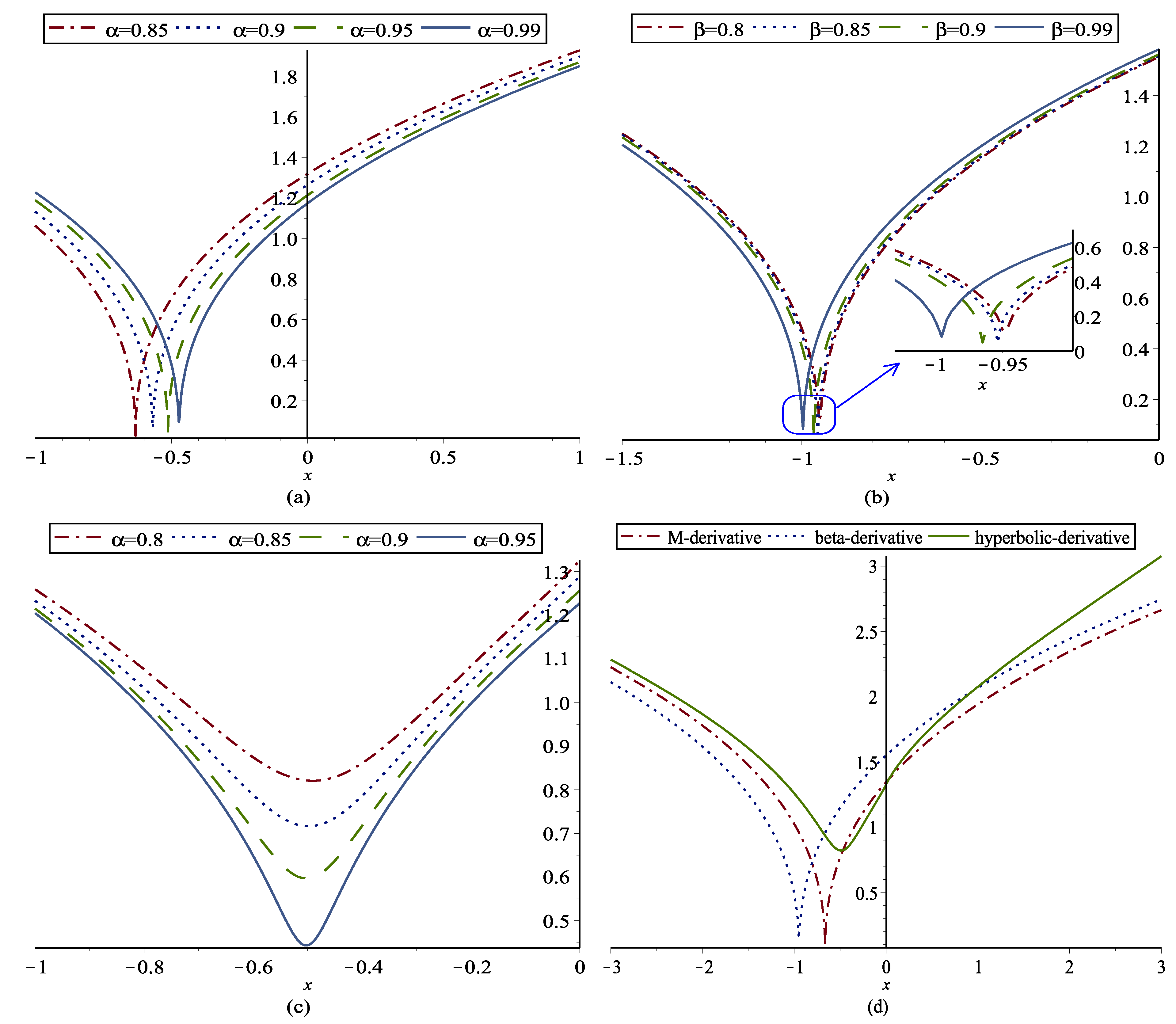
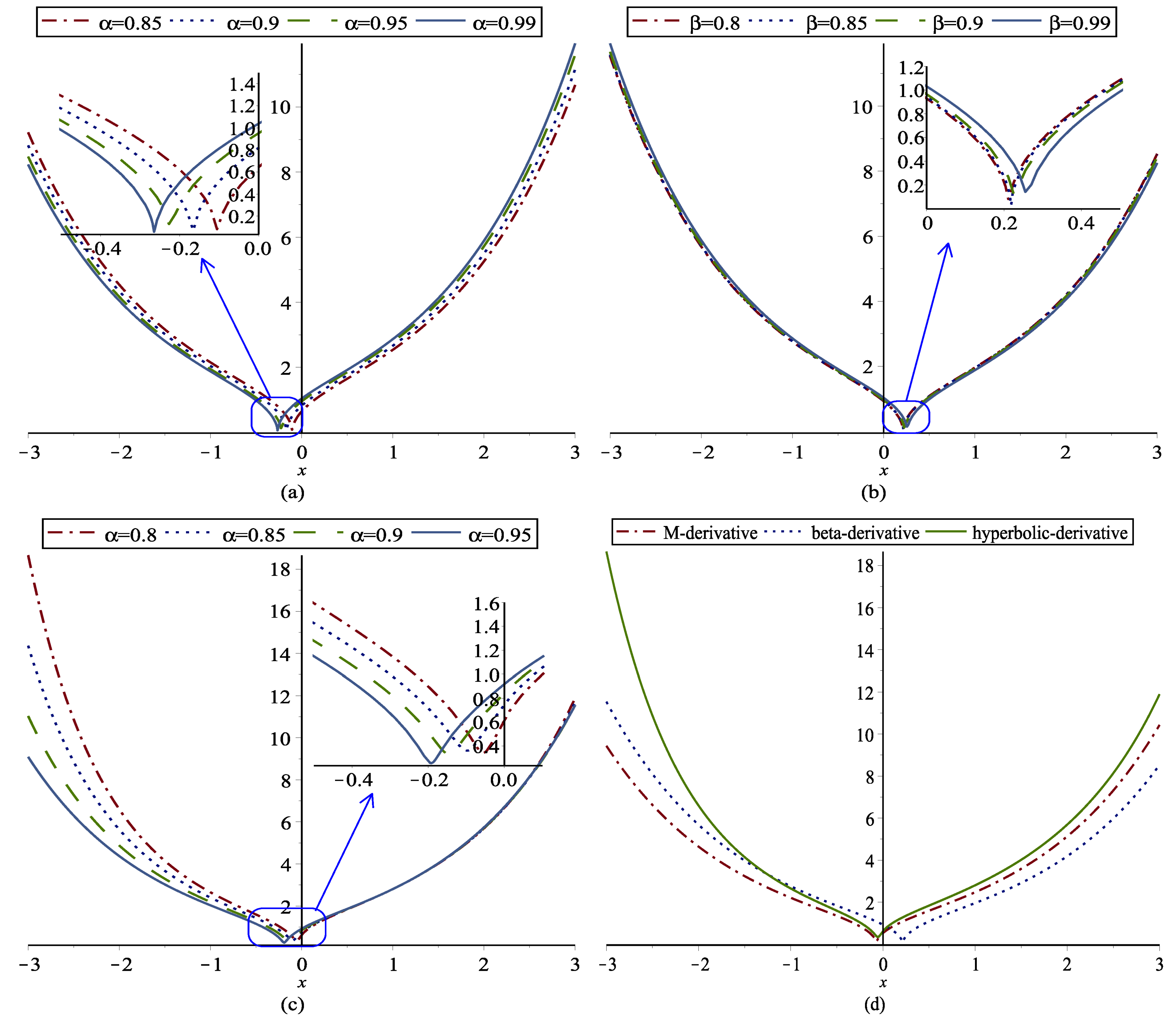
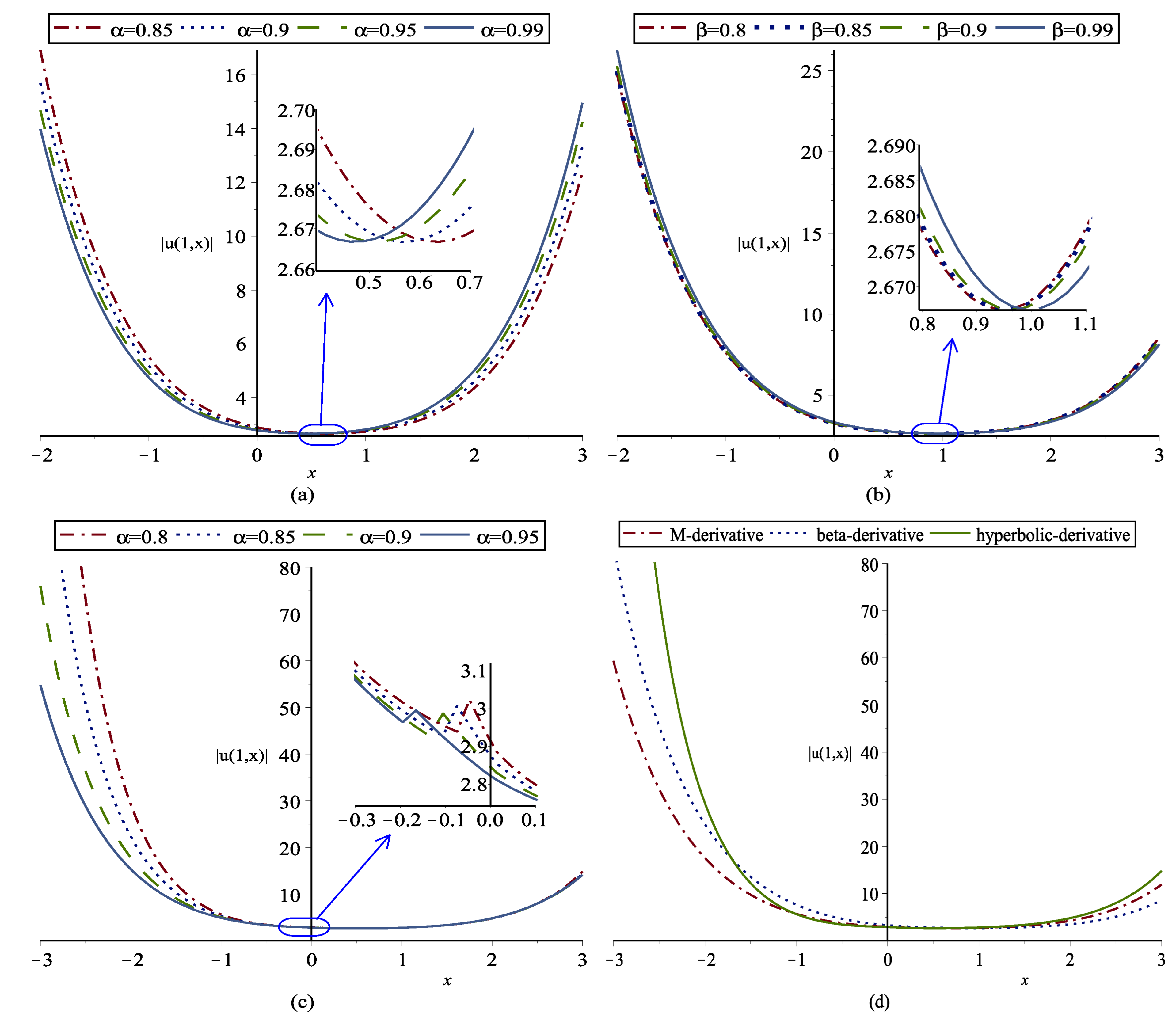
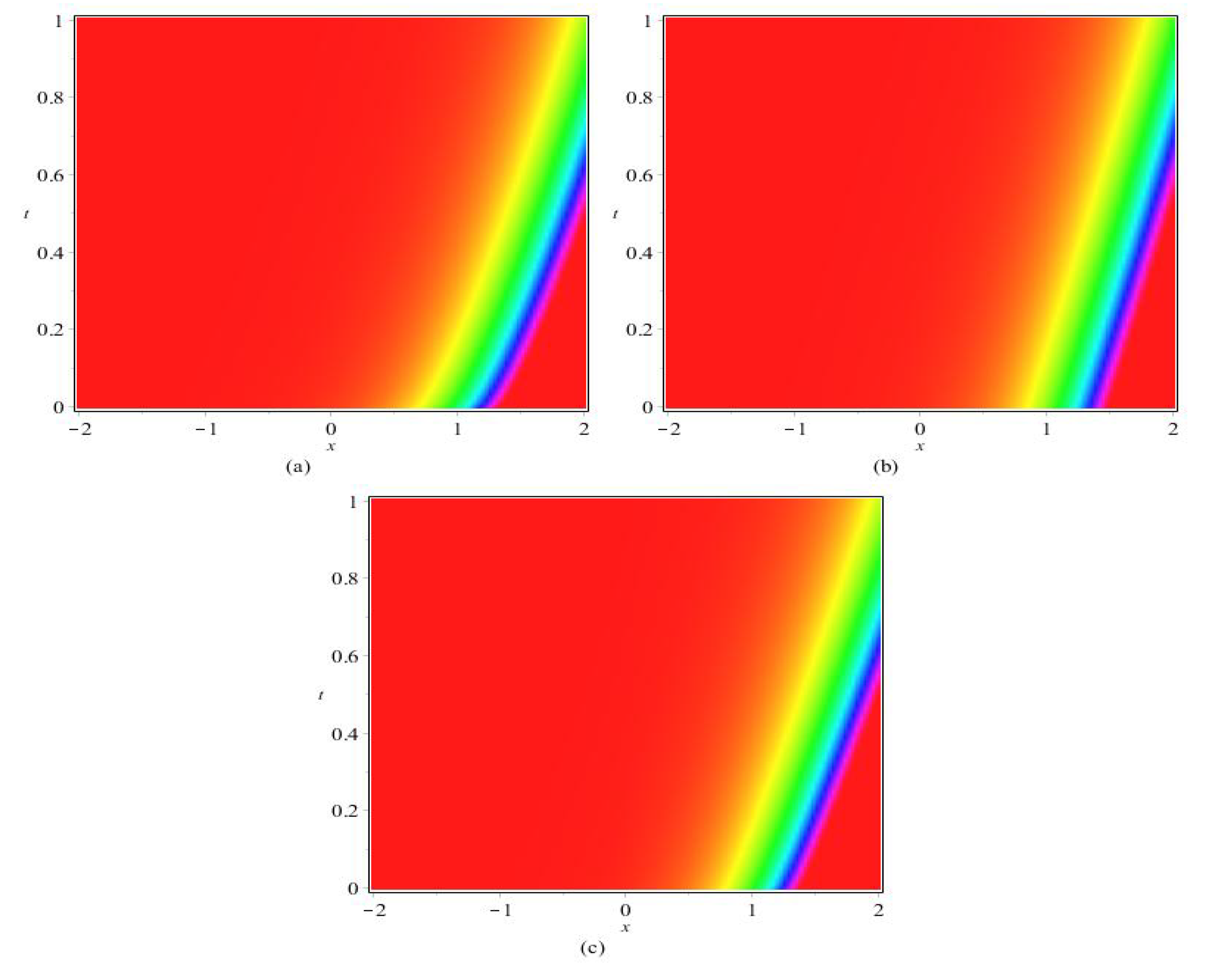
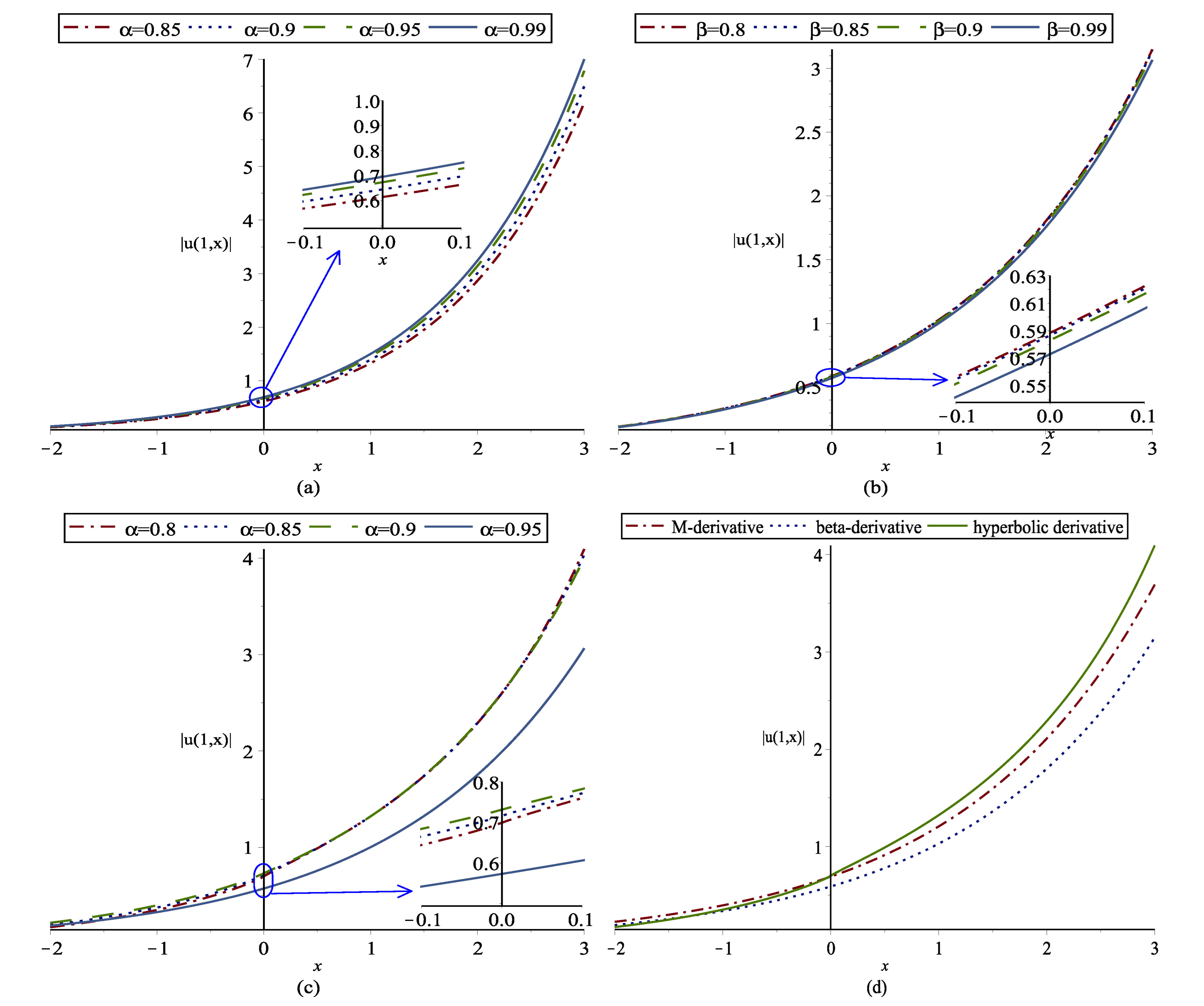
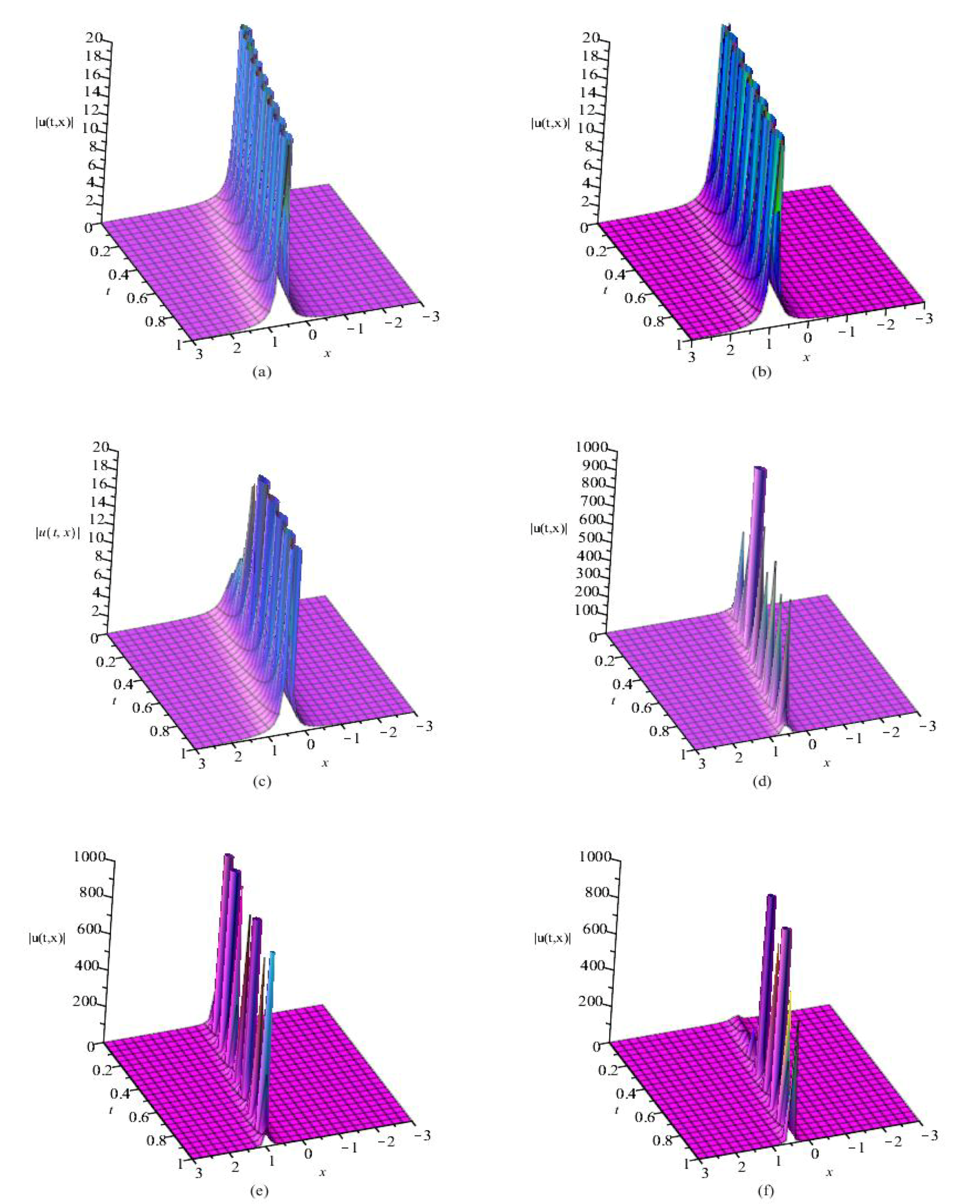
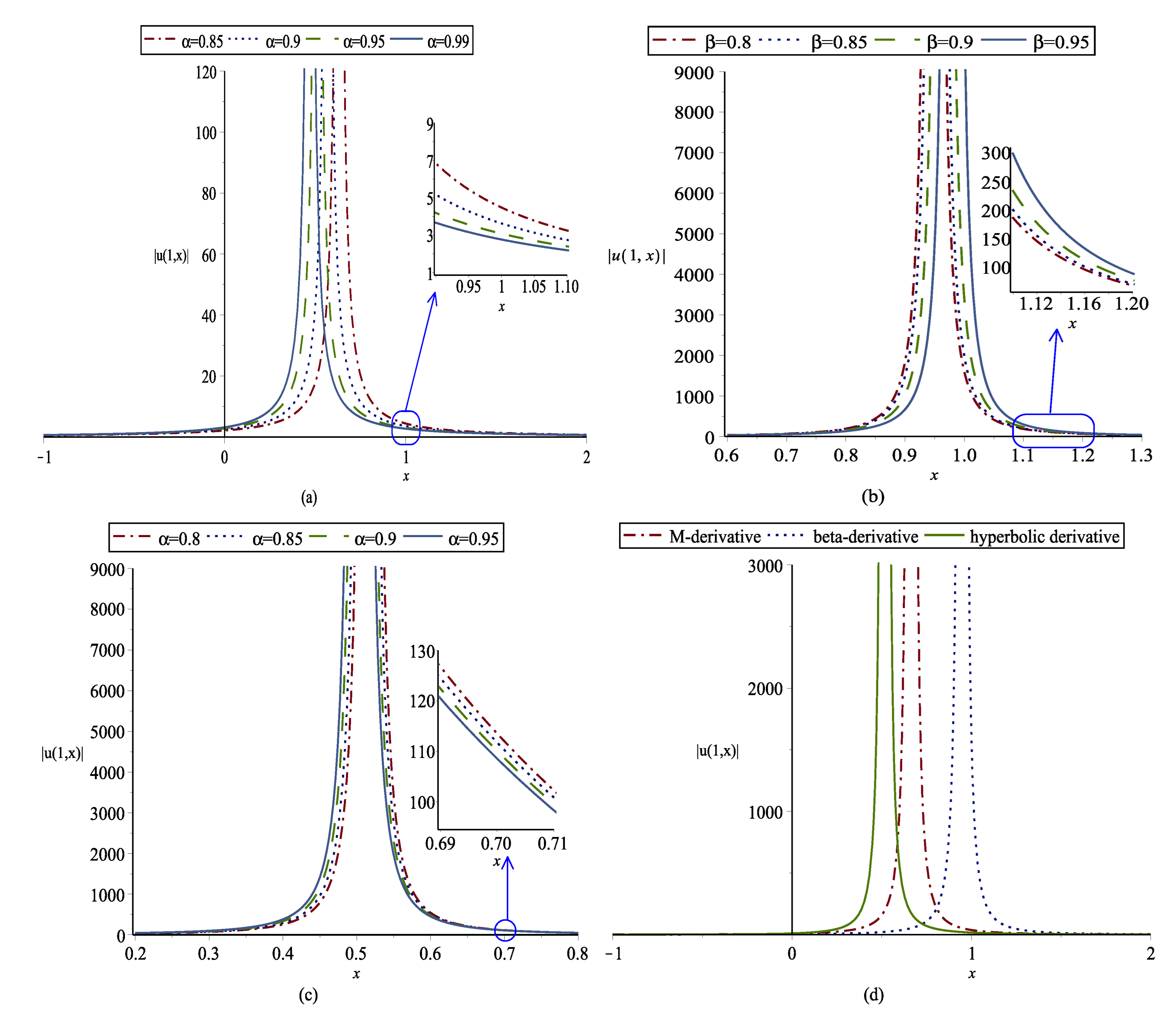
In this section, we consider the nonlinear s dimensional mK(m,n) equation with the mentioned temporal local derivative. By using some forthcoming transformations, this equation can be converted into a nonlinear ordinary differential equation. Then, using Nucci’s reduction technique, different types of exact solution can be extracted. All computations are accomplished by the Maple software.
Among the existence methods used to obtain exact solutions to differential equations, most of them extract special solutions such as hyperbolic solutions, soliton solutions, exponential solutions, etcetera. However, there are some analytical approaches, which can obtain different types of exact solutions, such as Lie symmetry method, invariant subspace method and the one utilized by us, the Nucci’s reduction method [54,55,56,57]. This point motivated our use of the reduction method to obtain exact solutions to Equation (3) with different differential operators.
Let us assume the s dimensional mK(m,n) Equation (3) with three local derivatives and the following corresponding transformations:
W ( θ ) = u ( t , x 1 , , x s ) , θ = i = 1 s k i x i c α Γ ( β + 1 ) t α ,
W ( θ ) = u ( t , x 1 , , x s ) , θ = i = 1 s k i x i 1 β c t + 1 Γ ( β ) β .
and
W ( θ ) = u ( t , x 1 , , x s ) , θ = 2 1 α 2 S i n h ( 1 α ) i = 1 s k i x i 1 + α 2 c t 1 + α 2 ,
for the M-derivative, beta-derivative and hyperbolic derivative, respectively. These transformations can convert the Equation (3) with fractional derivatives, into an ordinary differential equation with integer differential operator. Transformations (4)–(6) are developed in [40,50,58].
Let us first consider the s dimensional mK(n,n) equation, that is, m = n .
Applying transformations (4)–(6), we obtain the following single non-linear third-order ODE:
( c + a k 1 n ) W n 1 W + n W n 1 W + 3 n ( n 1 ) W n 2 W W + n ( n 1 ) ( n 2 ) W n 3 ( W ) 3 × i = 1 s α i k i 3 = 0 .
If we assume the change of variables [43,55,59,60]:
ψ 1 ( θ ) = W ( θ ) , ψ 2 ( θ ) = W ( θ ) , ψ 3 ( θ ) = W ( θ ) ,
then Equation (7) reduces into the following autonomous system of equations:
d ψ 1 d θ = ψ 2 , d ψ 2 d θ = ψ 3 , d ψ 3 d θ = ψ 2 n i = 1 s α i k i 3 n ( 1 n ) ( n 2 ) ( i = 1 s α i k i 3 ) ψ 2 2 ψ 1 2 + 3 n ( 1 n ) ( i = 1 s α i k i 3 ) ψ 3 ψ 1 + ( c + a k 1 n ) .
Selecting ψ 1 as a new independent variable converts the system (9) into
d ψ 2 d ψ 1 = ψ 3 ψ 2 , d ψ 3 d ψ 1 = 1 n i = 1 s α i k i 3 n ( 1 n ) ( n 2 ) ( i = 1 s α i k i 3 ) ψ 2 2 ψ 1 2 + 3 n ( 1 n ) ( i = 1 s α i k i 3 ) ψ 3 ψ 1 + ( c + a k 1 n ) .
From the first equation in (10), we have
ψ 3 = ψ 2 d ψ 2 d ψ 1 .
Therefore, the second equation of (10) can be written as:
d ψ 2 d ψ 1 2 + ψ 2 d 2 ψ 2 d ψ 1 2 = 1 n i = 1 s α i k i 3 n ( 1 n ) ( n 2 ) ( i = 1 s α i k i 3 ) ψ 2 2 ψ 1 2 + 3 n ( 1 n ) ( i = 1 s α i k i 3 ) ψ 2 ψ 1 d ψ 2 d ψ 1 + ( c + a k 1 n ) .
Solving Equation (11) concludes
ψ 2 ( ψ 1 ) = ± ψ 1 n 2 n ( i = 1 s α i k i 3 ) 2 ψ 1 n λ 1 n 2 ( i = 1 s α i k i 3 ) 2 λ 2 n 2 ( i = 1 s α i k i 3 ) + ψ 1 n ( c + a k 1 n ) ψ 1 n 2 n 2 ( i = 1 s α i k i 3 ) ,
with λ 1 and λ 2 arbitrary constants. Hence, the first equation of (9) has the following form:
d ψ 1 d θ = ± ψ 1 n 2 n ( i = 1 s α i k i 3 ) 2 ψ 1 n λ 1 n 2 ( i = 1 s α i k i 3 ) 2 λ 2 n 2 ( i = 1 s α i k i 3 ) + ψ 1 n ( c + a k 1 n ) ψ 1 n 2 n 2 ( i = 1 s α i k i 3 ) .
This equation is a separable ODE with an implicit general solution
θ n 2 ψ 1 n 2 ( θ ) n ψ 1 2 n ( θ ) ( c + a n k 1 ) + 2 ψ 1 n ( θ ) ( i = 1 s α i k i 3 ) λ 2 n 2 2 ( i = 1 s α i k i 3 ) λ 1 n 2 ψ 1 2 ( θ ) ( i = 1 s α i k i 3 ) d ψ 1 ( θ ) + λ 3 = 0 ,
where λ 3 is an arbitrary constant. To extract explicit solutions, we consider some special cases.
Case 1: λ 1 = 0 , k 1 = c a n
In this case, the integral in Equation (14) is solvable and we obtain
θ 2 n ψ 1 n 1 ( θ ) 2 λ 2 n 3 ψ 1 n 2 ( θ ) + λ 3 = 0 ,
which, after solving this equation regarding the dependent variable ψ 1 , concludes
W ( θ ) = ψ 1 ( θ ) = e ln n λ 2 2 ( θ + λ 3 ) 2 n .
Finally, from the obtained solution and transformations (4)–(6), we obtain the final solutions:
u ( t , x 1 , , x s ) = e ln n λ 2 2 ( i = 1 s k i x i c α Γ ( β + 1 ) t α + λ 3 ) 2 n ,
u ( t , x 1 , , x s ) = e ln n λ 2 2 ( i = 1 s k i x i 1 β c t + 1 Γ ( β ) β + λ 3 ) 2 n ,
u ( t , x 1 , , x s ) = e ln n λ 2 2 ( 2 1 α 2 S i n h ( 1 α ) i = 1 s k i x i 1 + α 2 c t 1 + α 2 + λ 3 ) 2 n ,
for s dimensional mK(n,n) equation with M-derivative, beta-derivative and hyperbolic derivative, respectively.
In Figure 1, density plots of the obtained exact solutions (15)–(17) are plotted with the same parameters and derivative orders but different types of derivatives. This figure shows that the type of local derivative effects the final results and solution profiles. Variations in local derivative orders and a comparison of the final solutions with three types of derivatives in the fixed time direction t = 1 , are plotted in Figure 2. We have to note that the figures are corresponding to the one-dimensional mK(n,n) equation, namely, s = 1 . This is very easy to plot in higher-dimensional cases s > 1 .
Case 2: λ 1 = 0 , k 1 = i = 1 s α i k i 3 c 2 a , n = 2
In this case, the Equation (14) reduces into
θ 2 ln ψ 1 2 ( θ ) + ψ 1 4 ( θ ) + 8 λ 2 + λ 3 = 0 ,
which solving this equation with respect to the dependent variable ψ 1 , yields
W ( θ ) = ψ 1 ( θ ) = ± 2 e 2 2 θ + λ 3 e 2 2 θ + λ 3 2 8 λ 2 2 e 2 2 θ + λ 3 .
Therefore, from the obtained solution and transformations (4)–(6), we can obtain the final solutions:
u ( t , x 1 , , x s ) = ± 2 e 2 2 i = 1 s k i x i c α Γ ( β + 1 ) t α + λ 3 e 2 2 i = 1 s k i x i c α Γ ( β + 1 ) t α + λ 3 2 8 λ 2 2 e 2 2 i = 1 s k i x i c α Γ ( β + 1 ) t α + λ 3 ,
u ( t , x 1 , , x s ) = ± 2 e 2 2 i = 1 s k i x i 1 β c t + 1 Γ ( β ) β + λ 3 e 2 2 i = 1 s k i x i 1 β c t + 1 Γ ( β ) β + λ 3 2 8 λ 2 2 e 2 2 i = 1 s k i x i 1 β c t + 1 Γ ( β ) β + λ 3 ,
and
u ( t , x 1 , , x s ) = ± 2 e 2 2 2 1 α 2 S i n h ( 1 α ) i = 1 s k i x i 1 + α 2 c t 1 + α 2 + λ 3 e 2 2 2 1 α 2 S i n h ( 1 α ) i = 1 s k i x i 1 + α 2 c t 1 + α 2 + λ 3 2 8 λ 2 2 e 2 2 2 1 α 2 S i n h ( 1 α ) i = 1 s k i x i 1 + α 2 c t 1 + α 2 + λ 3 ,
for s dimensional mK(n,n) equation with M-derivative, beta-derivative and hyperbolic derivative, respectively.
In Figure 3, density plots of the obtained exact solutions (18)–(20) are plotted with the same parameters and derivative orders but different type of derivatives. Variations in local derivative orders and a comparison of the final solutions with three types of derivatives in the fixed time direction t = 1 , are plotted in Figure 4.
Case 3: n = 1
In this case, the integral in Equation (14) is solvable, and we can obtain
θ + i = 1 s α i k i 3 a k 1 + c arctan λ 1 i = 1 s α i k i 3 ( a k 1 + c ) ψ 1 ( θ ) ( a k 1 + c ) 2 λ 1 i = 1 s α i k i 3 ψ 1 ( θ ) ( a k 1 + c ) ψ 1 2 ( θ ) 2 λ 2 i = 1 s α i k i 3 + λ 3 = 0 ,
which, solving this equation with respect to the dependent variable ψ 1 , yields
W ( θ ) = ψ 1 ( θ ) = 1 a k 1 + c [ i = 1 s α i k i 3 ( 2 ( a k 1 + c ) λ 2 λ 1 2 i = 1 s α i k i 3 ) cos 2 a k 1 + c i = 1 s α i k i 3 ( θ + λ 3 ) 1 + λ 1 i = 1 s α i k i 3 ] .
Lastly, from the obtained solution and transformations (4)–(6) we obtain the final solutions:
u K ( t , x 1 , , x s ) = 1 a k 1 + c [ ( i = 1 s α i k i 3 ) ϑ sin 2 a k 1 + c i = 1 s α i k i 3 ( θ K + λ 3 ) + λ 1 i = 1 s α i k i 3 ] ,
where ϑ = λ 1 2 i = 1 s α i k i 3 2 ( a k 1 + c ) λ 2 , θ K { θ 1 , θ 2 , θ 3 } , and
θ 1 = i = 1 s k i x i c α Γ ( β + 1 ) t α , θ 2 = i = 1 s k i x i 1 β c t + 1 Γ ( β ) β , θ 3 = 2 1 α 2 S i n h ( 1 α ) i = 1 s k i x i 1 + α 2 c t 1 + α 2 ,
corresponding to M-derivative, beta-derivative and hyperbolic derivative, respectively.
Density plots and 2-D plots of (21) with three types of local derivatives are plotted in Figure 5 and Figure 6, respectively.
Case 4: λ 1 0 , λ 2 0 , n R +
In this case, the integral in Equation (14) is solvable and we can obtain
θ n 2 γ n ( a k 1 n + c ) ln ( ψ 1 ( θ ) ) + λ 3 = 0 ,
which, solving this equation with respect to the dependent variable ψ 1 , concludes the final solution
W ( θ ) = ψ 1 ( θ ) = e ± n ( a k 1 n + c ) i = 1 s α i k i 3 × θ + λ 3 n 2 .
Lastly, from the obtained solution and transformations (4)–(6), we obtain the final solutions:
u ( t , x 1 , , x s ) = e ± n ( a k 1 n + c ) i = 1 s α i k i 3 × i = 1 s k i x i c α Γ ( β + 1 ) t α + λ 3 n 2 ,
u ( t , x 1 , , x s ) = e ± n ( a k 1 n + c ) i = 1 s α i k i 3 × i = 1 s k i x i 1 β c t + 1 Γ ( β ) β + λ 3 n 2 ,
and
u ( t , x 1 , , x s ) = e ± n ( a k 1 n + c ) i = 1 s α i k i 3 × 2 1 α 2 S i n h ( 1 α ) i = 1 s k i x i 1 + α 2 c t 1 + α 2 + λ 3 n 2 ,
corresponding to M-derivative, beta-derivative and hyperbolic derivative, respectively.
Figure 7, shows the density plots of (22)–(24), and corresponding 2-D plots are demonstrated in Figure 8.
Case 5: m n
In order to show the power of method, we tried to find exact solutions of the mK(m,n) equation with local derivatives as follows:
u n 1 D t u + a ( u m ) x + ( u n ) x x x = 0 , D t { 0 A D t β , M D t α , β , D h α } ,
whenever m n .
Applying transformations (4)–(6), we obtain the following single nonlinear third-order ODE w.r.t. n and m:
( c + a k 1 m ) W m 1 W + n W n 1 W + 3 n ( n 1 ) W n 2 W W + n ( n 1 ) ( n 2 ) W n 3 ( W ) 3 × i = 1 s α i k i 3 = 0 .
Let us assume the change of variables
ψ 1 ( θ ) = W ( θ ) , ψ 2 ( θ ) = W ( θ ) , ψ 3 ( θ ) = W ( θ ) .
By assuming (8), the Equation (26) reduces into the following autonomous system of equations:
d ψ 1 d θ = ψ 2 , d ψ 2 d θ = ψ 3 , d ψ 3 d θ = ψ 2 n i = 1 s α i k i 3 n ( 1 n ) ( n 2 ) ( i = 1 s α i k i 3 ) ψ 2 2 ψ 1 2 + 3 n ( 1 n ) ( i = 1 s α i k i 3 ) ψ 3 ψ 1 + ( c + a k 1 m ) ψ 1 m n .
Selecting ψ 1 as a new independent variable, converts the system (27) into
d ψ 2 d ψ 1 = ψ 3 ψ 2 , d ψ 3 d ψ 1 = 1 n i = 1 s α i k i 3 n ( 1 n ) ( n 2 ) ( i = 1 s α i k i 3 ) ψ 2 2 ψ 1 2 + 3 n ( 1 n ) ( i = 1 s α i k i 3 ) ψ 3 ψ 1 + ( c + a k 1 m ) ψ 1 m n .
From the first equation in (28), we have
ψ 3 = ψ 2 d ψ 2 d ψ 1 .
Therefore, the second equation of (28) can be written as:
d ψ 2 d ψ 1 2 + ψ 2 d 2 ψ 2 d ψ 1 2 = 1 n i = 1 s α i k i 3 × n ( 1 n ) ( n 2 ) ( i = 1 s α i k i 3 ) ψ 2 2 ψ 1 2 + 3 n ( 1 n ) ( i = 1 s α i k i 3 ) ψ 2 ψ 1 d ψ 2 d ψ 1 + ( c + a k 1 m ) ψ 1 m n .
Solving Equation (30) concludes
ψ 2 ( ψ 1 ) = ± m n ( m + n ) ϱ ψ 1 2 ( n 1 ) + ( a k 1 m + c ) ψ 1 m + n λ 1 m ( m + n ) ϱ ψ 1 n + λ 2 m ( m + n ) ϱ m n ( m + n ) ϱ ψ 1 2 ( n 1 ) ,
where ϱ = i = 1 s α i k i 3 , and λ 1 and λ 2 are arbitrary constants. Hence, the first equation of (27) yields
d ψ 1 d θ = ± m n ( m + n ) ϱ ψ 1 2 ( n 1 ) + ( a k 1 m + c ) ψ 1 m + n λ 1 m ( m + n ) ϱ ψ 1 n + λ 2 m ( m + n ) ϱ m n ( m + n ) ϱ ψ 1 2 ( n 1 ) .
This equation is a separable ordinary differential equation. Therefore, we obtain
θ 2 m n ( m + n ) ϱ ψ 1 n 1 ( m n ) m n ( m + n ) ( c + a k 1 m ) ϱ ψ 1 m + n 2 + λ 3 = 0 ,
where λ 1 = λ 2 = 0 , and λ 3 is an arbitrary constant.
Solving this equation concludes:
W ( θ ) = ψ 1 ( θ ) = e ln 2 m n ( m + n ) ϱ ( m n ) 2 ( c + a k 1 m ) ( θ + λ 3 ) 2 m n .
Hence, from the obtained solution and transformations (4)–(6), we obtain the final solutions:
u ( t , x 1 , , x s ) = e ln 2 m n ( m + n ) ϱ ( m n ) 2 ( c + a k 1 m ) ( i = 1 s k i x i c α Γ ( β + 1 ) t α + λ 3 ) 2 m n ,
u ( t , x 1 , , x s ) = e ln 2 m n ( m + n ) ϱ ( m n ) 2 ( c + a k 1 m ) ( i = 1 s k i x i 1 β c t + 1 Γ ( β ) β + λ 3 ) 2 m n ,
and
u ( t , x 1 , , x s ) = e ln 2 m n ( m + n ) ϱ ( m n ) 2 ( c + a k 1 m ) ( 2 1 α 2 S i n h ( 1 α ) i = 1 s k i x i 1 + α 2 c t 1 + α 2 + λ 3 ) 2 m n ,
corresponding to M-derivative, beta-derivative and hyperbolic derivative, respectively.
Soliton-type solutions (34)–(36) with different values of derivative orders and non-linearity power are plotted in Figure 9. Corresponding 2-D plots are demonstrated in Figure 10.

4. Conclusions

In this paper, an important differential equation, namely, the higher-order generalized nonlinear dispersive mK(m,n) equation is considered with different values of m and n. The supposed derivatives in the time direction are M-derivative, beta-derivative and hyperbolic local derivative. Different types of soliton solutions in five cases, are extracted using Nucci’s reduction method. A comparison of the obtained solutions with various local derivatives is graphically considered. In the literature, to the best knowledge of the author of this article, the reduction method is novel for the differential equations with local derivatives. Therefore, this paper can serve as a starting point for future works on local derivatives of other physical models.

Author Contributions

Conceptualization, M.S.H.; formal analysis, A.A.; investigation, A.A. and M.S.H.; methodology, F.J.; resources, F.J. All authors have read and agreed to the published version of the manuscript.

Funding

This work was supported by the Natural Science Foundation of Hunan province (Grant Nos.: 2018JJ3018, 17C0292).

Institutional Review Board Statement

Not applicable.

Informed Consent Statement

Not applicable.

Data Availability Statement

The data presented in this study are available within the article.

Conflicts of Interest

The authors declare no conflict of interest.

References

  1. Wang, F.; Khan, M.N.; Ahmad, I.; Ahmad, H.; Abu-Zinadah, H.; Chu, Y.M. Numerical Solution of Traveling Waves in Chemical Kinetics: Time Fractional Fishers Equations. Fractals 2022, 30, 2240051. [Google Scholar] [CrossRef]
  2. Rashid, S.; Abouelmagd, E.I.; Khalid, A.; Farooq, F.B.; Chu, Y.M. Some Recent Developments on Dynamical -Discrete Fractional Type Inequalities in the Frame of Nonsingular and Nonlocal Kernels. Fractals 2021, 30, 2240110. [Google Scholar] [CrossRef]
  3. Jin, F.; Qian, Z.S.; Chu, Y.M.; ur Rahman, M. On nonlinear evolution model for drinking behavior under caputo-fabrizio derivative. J. Appl. Anal. Comput. 2022, 12, 790–806. [Google Scholar] [CrossRef]
  4. He, Z.Y.; Abbes, A.; Jahanshahi, H.; Alotaibi, N.D.; Wang, Y. Fractional-Order Discrete-Time SIR Epidemic Model with Vaccination: Chaos and Complexity. Mathematics 2022, 10, 165. [Google Scholar] [CrossRef]
  5. Hajiseyedazizi, S.N.; Samei, M.E.; Alzabut, J.; Chu, Y.M. On multi-step methods for singular fractional q-integro-differential equations. Open Math. 2021, 19, 1378–1405. [Google Scholar] [CrossRef]
  6. Zhao, T.H.; Zhou, B.C.; Wang, M.K.; Chu, Y.M. On approximating the quasi-arithmetic mean. J. Inequalities Appl. 2019, 2019, 42. [Google Scholar] [CrossRef]
  7. Sapuppo, F.; Schembri, F.; Fortuna, L.; Bucolo, M. Microfluidic circuits and systems. IEEE Circuits Syst. Mag. 2009, 9, 6–19. [Google Scholar] [CrossRef]
  8. Sapuppo, F.; Schembri, F.; Fortuna, L.; Llobera, A.; Bucolo, M. A polymeric micro-optical system for the spatial monitoring in two-phase microfluidics. Microfluid. Nanofluidics 2012, 12, 165–174. [Google Scholar] [CrossRef]
  9. Hashemi, M.S.; Baleanu, D. Lie symmetry analysis and exact solutions of the time fractional Gas dynamics equation. J. Optoelectron. Adv. Mater 2016, 18, 383–388. [Google Scholar]
  10. Osman, M.S.; Baleanu, D.; Adem, A.R.; Hosseini, K.; Mirzazadeh, M.; Eslami, M. Double-wave solutions and Lie symmetry analysis to the (2+ 1)-dimensional coupled Burgers equations. Chin. J. Phys. 2020, 63, 122–129. [Google Scholar] [CrossRef]
  11. Hashemi, M.S.; Haji-Badali, A.; Vafadar, P. Group invariant solutions and conservation laws of the Fornberg–Whitham equation. Z. Für Naturforschung A 2014, 69, 489–496. [Google Scholar] [CrossRef]
  12. Inc, M.; Yusuf, A.; Isa, A.A.; Hashemi, M.S. Soliton solutions, stability analysis and conservation laws for the brusselator reaction diffusion model with time-and constant-dependent coefficients. Eur. Phys. J. Plus 2018, 133, 168. [Google Scholar] [CrossRef]
  13. Hashemi, M.S. Invariant subspaces admitted by fractional differential equations with conformable derivatives. Chaos Solitons Fractals 2018, 107, 161–169. [Google Scholar] [CrossRef]
  14. Qu, C.; Zhu, C. Classification of coupled systems with two-component nonlinear diffusion equations by the invariant subspace method. J. Phys. A Math. Theor. 2009, 42, 475201. [Google Scholar] [CrossRef]
  15. Yusuf, A. Symmetry analysis, invariant subspace and conservation laws of the equation for fluid flow in porous media. Int. J. Geom. Methods Mod. Phys. 2020, 17, 2050173. [Google Scholar] [CrossRef]
  16. Bekir, A.; Kaplan, M. Exponential rational function method for solving nonlinear equations arising in various physical models. Chin. J. Phys. 2016, 54, 365–370. [Google Scholar] [CrossRef]
  17. Akbulut, A.; Kaplan, M.; Kaabar, M.K.A. New conservation laws and exact solutions of the special case of the fifth-order KdV equation. J. Ocean. Eng. Sci. 2021. [Google Scholar] [CrossRef]
  18. Iqbal, M.A.; Wang, Y.; Miah, M.M.; Osman, M.S. Study on Date–Jimbo–Kashiwara–Miwa Equation with Conformable Derivative Dependent on Time Parameter to Find the Exact Dynamic Wave Solutions. Fractal Fract. 2022, 6, 4. [Google Scholar] [CrossRef]
  19. Arnous, A.H.; Mirzazadeh, M.; Zhou, Q.; Moshokoa, S.P.; Biswas, A.; Belic, M. Soliton solutions to resonant nonlinear schrodinger’s equation with time-dependent coefficients by modified simple equation method. Optik 2016, 127, 11450–11459. [Google Scholar] [CrossRef] [Green Version]
  20. Savaissou, N.; Gambo, B.; Rezazadeh, H.; Bekir, A.; Doka, S.Y. Exact optical solitons to the perturbed nonlinear Schrödinger equation with dual-power law of nonlinearity. Opt. Quantum Electron. 2020, 52, 318. [Google Scholar] [CrossRef]
  21. Pinar, Z.; Rezazadeh, H.; Eslami, M. Generalized logistic equation method for Kerr law and dual power law Schrödinger equations. Opt. Quantum Electron. 2020, 52, 504. [Google Scholar] [CrossRef]
  22. Inc, M.; Hosseini, K.; Samavat, M.; Mirzazadeh, M.; Eslami, M.; Moradi, M.; Baleanu, D. N-wave and other solutions to the B-type Kadomtsev-Petviashvili equation. Therm. Sci. 2019, 23, 2027–2035. [Google Scholar] [CrossRef] [Green Version]
  23. Rezazadeh, H.; Inc, M.; Baleanu, D. New solitary wave solutions for variants of (3+ 1)-dimensional Wazwaz-Benjamin-Bona-Mahony equations. Front. Phys. 2020, 8, 332. [Google Scholar] [CrossRef]
  24. Zahran, E.H.M.; Khater, M.M. Modified extended tanh-function method and its applications to the Bogoyavlenskii equation. Appl. Math. Model. 2016, 40, 1769–1775. [Google Scholar] [CrossRef]
  25. Akbulut, A.; Taşcan, F. Application of conservation theorem and modified extended tanh-function method to (1 + 1)-dimensional nonlinear coupled Klein–Gordon–Zakharov equation. Chaos Solitons Fractals 2017, 104, 33–40. [Google Scholar] [CrossRef]
  26. Zafar, A.; Raheel, M.; Asif, M.; Hosseini, K.; Mirzazadeh, M.; Akinyemi, L. Some novel integration techniques to explore the conformable M-fractional Schrödinger-Hirota equation. J. Ocean. Eng. Sci. 2021. [Google Scholar] [CrossRef]
  27. Rezazadeh, H.; Seadawy, A.R.; Eslami, M.; Mirzazadeh, M. Generalized solitary wave solutions to the time fractional generalized Hirota-Satsuma coupled KdV via new definition for wave transformation. J. Ocean Eng. Sci. 2019, 4, 77–84. [Google Scholar] [CrossRef]
  28. Ma, W.X. Riemann–Hilbert problems and N-soliton solutions for a coupled mKdV system. J. Geom. Phys. 2018, 132, 45–54. [Google Scholar] [CrossRef]
  29. Ma, W.X. N-soliton solution and the Hirota condition of a (2 + 1)-dimensional combined equation. Math. Comput. Simul. 2021, 190, 270–279. [Google Scholar] [CrossRef]
  30. Li, J.; Xia, T. N-soliton solutions for the nonlocal Fokas–Lenells equation via RHP. Appl. Math. Lett. 2021, 113, 106850. [Google Scholar] [CrossRef]
  31. Wazwaz, A.M. Kadomtsev–Petviashvili hierarchy: N-soliton solutions and distinct dispersion relations. Appl. Math. Lett. 2016, 52, 74–79. [Google Scholar] [CrossRef]
  32. Dong, H.; Wei, C.; Zhang, Y.; Liu, M.; Fang, Y. The Darboux Transformation and N-Soliton Solutions of Coupled Cubic-Quintic Nonlinear Schrödinger Equation on a Time-Space Scale. Fractal Fract. 2021, 6, 12. [Google Scholar] [CrossRef]
  33. Jiang, Z.; Zhang, Z.G.; Li, J.J.; Yang, H.W. Analysis of Lie symmetries with conservation laws and solutions of generalized (4 + 1)-dimensional time-fractional Fokas equation. Fractal Fract. 2022, 6, 108. [Google Scholar] [CrossRef]
  34. Sun, Y.L.; Ma, W.X.; Yu, J.P. N-soliton solutions and dynamic property analysis of a generalized three-component Hirota–Satsuma coupled KdV equation. Appl. Math. Lett. 2021, 120, 107224. [Google Scholar] [CrossRef]
  35. Rosenau, P.; Hyman, J.M. Compactons: Solitons with finite wavelength. Phys. Rev. Lett. 1993, 70, 564. [Google Scholar] [CrossRef] [PubMed]
  36. Niu, Z.; Wang, Z. Bifurcation and exact traveling wave solutions for the generalized nonlinear dispersive mk (m, n) equation. J. Appl. Anal. Comput. 2021, 11, 2866–2875. [Google Scholar] [CrossRef]
  37. Wazwaz, A.M. General compactons solutions and solitary patterns solutions for modified nonlinear dispersive equations mK (n, n) in higher dimensional spaces. Math. Comput. Simul. 2002, 59, 519–531. [Google Scholar] [CrossRef]
  38. He, B.; Meng, Q.; Rui, W.; Long, Y. Bifurcations of travelling wave solutions for the mK (n, n) equation. Commun. Nonlinear Sci. Numer. Simul. 2008, 13, 2114–2123. [Google Scholar] [CrossRef]
  39. Yan, Z. Modified nonlinearly dispersive mK (m, n, k) equations: I. New compacton solutions and solitary pattern solutions. Comput. Phys. Commun. 2003, 152, 25–33. [Google Scholar] [CrossRef]
  40. Yépez-Martínez, H.; Rezazadeh, H.; Inc, M.; Akinlar, M.A. New solutions to the fractional perturbed Chen–Lee–Liu equation with a new local fractional derivative. Waves Random Complex Media 2021, 1–36. [Google Scholar] [CrossRef]
  41. Yang, X.J. Advanced Local Fractional Calculus and Its Applications; World Science Publisher: Singapore, 2012. [Google Scholar]
  42. Kolwankar, K.M.; Gangal, A.D. Fractional differentiability of nowhere differentiable functions and dimensions. Chaos Interdiscip. J. Nonlinear Sci. 1996, 6, 505–513. [Google Scholar] [CrossRef] [PubMed] [Green Version]
  43. Hashemi, M.S.; Baleanu, D. Lie Symmetry Analysis of Fractional Differential Equations; CRC Press: Boca Raton, FL, USA, 2020. [Google Scholar]
  44. Kilbas, A.A.; Srivastava, H.M.; Trujillo, J.J. Theory and Applications of Fractional Differential Equations; Elsevier: Amsterdam, The Netherlands, 2006; Volume 204. [Google Scholar]
  45. Podlubny, I. Fractional Differential Equations: An Introduction to Fractional Derivatives, Fractional Differential Equations, to Methods of Their Solution and Some of Their Applications; Elsevier: Amsterdam, The Netherlands, 1998. [Google Scholar]
  46. Yang, X.J.; Baleanu, D.; Srivastava, H.M. Local Fractional Integral Transforms and Their Applications; Academic Press: Cambridge, MA, USA, 2015. [Google Scholar]
  47. Adda, F.B.; Cresson, J. About non-differentiable functions. J. Math. Anal. Appl. 2001, 263, 721–737. [Google Scholar] [CrossRef] [Green Version]
  48. Kolwankar, K.M.; Gangal, A.D. Hölder exponents of irregular signals and local fractional derivatives. Pramana 1997, 48, 49–68. [Google Scholar] [CrossRef] [Green Version]
  49. Carpinteri, A.; Cornetti, P. A fractional calculus approach to the description of stress and strain localization in fractal media. Chaos Solitons Fractals 2002, 13, 85–94. [Google Scholar] [CrossRef]
  50. Sousa, J.; de Oliveira, E.C. On the local M-derivative. arXiv 2017, arXiv:1704.08186. [Google Scholar]
  51. Atangana, A.; Baleanu, D.; Alsaedi, A. Analysis of time-fractional Hunter-Saxton equation: A model of neumatic liquid crystal. Open Phys. 2016, 14, 145–149. [Google Scholar] [CrossRef]
  52. Salahshour, S.; Ahmadian, A.; Abbasbandy, S.; Baleanu, D. M-fractional derivative under interval uncertainty: Theory, properties and applications. Chaos Solitons Fractals 2018, 117, 84–93. [Google Scholar] [CrossRef]
  53. Khalil, R.; Al Horani, M.; Yousef, A.; Sababheh, M. A new definition of fractional derivative. J. Comput. Appl. Math. 2014, 264, 65–70. [Google Scholar] [CrossRef]
  54. Nucci, M.C. The complete Kepler group can be derived by Lie group analysis. J. Math. Phys. 1996, 37, 1772–1775. [Google Scholar] [CrossRef]
  55. Nucci, M.C.; Leach, P.L. The determination of nonlocal symmetries by the technique of reduction of order. J. Math. Anal. Appl. 2000, 251, 871–884. [Google Scholar] [CrossRef] [Green Version]
  56. Nucci, M.C.; Leach, P.G.L. An integrable SIS model. J. Math. Anal. Appl. 2004, 290, 506–518. [Google Scholar] [CrossRef] [Green Version]
  57. Marcelli, M.; Nucci, M.C. Lie point symmetries and first integrals: The Kowalevski top. J. Math. Phys. 2003, 44, 2111–2132. [Google Scholar] [CrossRef] [Green Version]
  58. Qureshi, S.; Chang, M.M.; Shaikh, A.A. Analysis of series RL and RC circuits with time-invariant source using truncated M, atangana beta and conformable derivatives. J. Ocean Eng. Sci. 2021, 6, 217–227. [Google Scholar] [CrossRef]
  59. Hashemi, M.S.; Nucci, M.C.; Abbasbandy, S. Group analysis of the modified generalized Vakhnenko equation. Commun. Nonlinear Sci. Numer. Simul. 2013, 18, 867–877. [Google Scholar] [CrossRef]
  60. Hashemi, M.S. A novel approach to find exact solutions of fractional evolution equations with non-singular kernel derivative. Chaos Solitons Fractals 2021, 152, 111367. [Google Scholar] [CrossRef]
Figure 1. Exact solutions with α 1 = a = c = 2 , λ 2 = λ 3 = 1 , m = 3 , and n = 5 , β = α = 0.9  w.r.t. (a) M-derivative (15), (b) beta-derivative (16), (c) hyperbolic-derivative (17).
Fractalfract 06 00202 g001
Figure 2. Exact solutions with α 1 = a = c = 2 , λ 2 = λ 3 = t = 1 , m = 3 , n = 5 , and (a) β = 0.9 , and various α w.r.t. M-derivative (15), (b) various β w.r.t. beta-derivative (16) (c) various α w.r.t. hyperbolic-derivative (17) (d) α = β = 0.8 , and various derivatives.
Fractalfract 06 00202 g002
Figure 3. Density plots with a = c = 2 , λ 2 = λ 3 = 1 , α 1 = 3 2 2 3 , m = 3 , and β = α = 0.9  w.r.t. (a) M-derivative (18), (b) beta-derivative (19), (c) hyperbolic-derivative (20).
Fractalfract 06 00202 g003
Figure 4. Exact solutions with a = c = 2 , λ 2 = λ 3 = t = 1 , α 1 = 3 2 2 3 , m = 3 , and (a) β = 0.9 , and various α w.r.t. M-derivative (18), (b) various β w.r.t. beta-derivative (19) (c) various α w.r.t. hyperbolic-derivative (20) (d) α = β = 0.8 , and various derivatives.
Fractalfract 06 00202 g004
Figure 5. Exact solutions with k 1 = α 1 = a = c = 2 , λ 1 = λ 2 = λ 3 = 1 , m = 3 , and n = 1.5 ,   β = α = 0.9  w.r.t. (a) M-derivative (21), (b) beta-derivative (c) hyperbolic-derivative.
Fractalfract 06 00202 g005
Figure 6. Exact solutions with k 1 = α 1 = a = c = 2 , λ 1 = λ 2 = λ 3 = t = 1 , m = 3 , and (a) n = 1.5 ,   β = 0.9 , and various α w.r.t. M-derivative (21), (b) n = 2 , and various β w.r.t. beta-derivative (21) (c) n = 2 , and various α w.r.t. hyperbolic-derivative (21) (d) n = 2 , α = β = 0.8 , and various derivatives in (21).
Fractalfract 06 00202 g006
Figure 7. Exact solutions with k 1 = α 1 = a = c = 2 , λ 3 = 1 , and (a) n = 0.5 , m = 2 , α = 0.8 , β = 0.9 , w.r.t. M-derivative (22), (b) n = 0.5 , m = 2 , β = 0.9 , w.r.t. beta-derivative (23), (c) n = 0.5 , m = 2 , α = 0.8 , w.r.t. hyperbolic-derivative (24).
Fractalfract 06 00202 g007
Figure 8. Exact solutions with k 1 = α 1 = a = c = 2 , λ 3 = t = 1 , m = 3 , and (a) n = 1.5 ,   β = 0.9 , and various α w.r.t. M-derivative (22), (b) n = 2 , and various β w.r.t. beta-derivative (23) (c) n = 2 , and various α w.r.t. hyperbolic-derivative (24) (d) n = 2 , α = β = 0.8 , and various derivatives in (22)–(24).
Fractalfract 06 00202 g008
Figure 9. Exact solutions with k 1 = α 1 = a = c = 2 , λ 3 = 1 , and (a) n = 0.5 , m = 2 , α = 0.8 , β = 0.9 , w.r.t. M-derivative (34), (b) n = 0.5 , m = 2 , β = 0.9 , w.r.t. beta-derivative (35), (c) n = 0.5 , m = 2 , α = 0.8 , w.r.t. hyperbolic-derivative (36), (d) n = 1.5 , m = 3 , α = β = 0.9 , w.r.t. M-derivative (34), (e) n = 1.5 , m = 3 , β = 0.9 , w.r.t. beta-derivative (35), (f) n = 1.5 , m = 3 , α = 0.9 , w.r.t. hyperbolic-derivative (36).
Fractalfract 06 00202 g009
Figure 10. Exact solutions with k 1 = α 1 = a = c = 2 , λ 3 = t = 1 , m = 3 , and (a) n = 1.5 ,   β = 0.9 , and various α w.r.t. M-derivative (34), (b) n = 2 , and various β w.r.t. beta-derivative (35) (c) n = 2 , and various α w.r.t. hyperbolic-derivative (36) (d) n = 2 ,   α = β = 0.8 , and various derivatives in (34)–(36).
Fractalfract 06 00202 g010
Publisher’s Note: MDPI stays neutral with regard to jurisdictional claims in published maps and institutional affiliations.

