Second-Order Time Stepping Scheme Combined with a Mixed Element Method for a 2D Nonlinear Fourth-Order Fractional Integro-Differential Equations

Abstract

In this article, we study a class of two-dimensional nonlinear fourth-order partial differential equation models with the Riemann–Liouville fractional integral term by using a mixed element method in space and the second-order backward difference formula (BDF2) with the weighted and shifted Grünwald integral (WSGI) formula in time. We introduce an auxiliary variable to transform the nonlinear fourth-order model into a low-order coupled system including two second-order equations and then discretize the resulting equations by the combined method between the BDF2 with the WSGI formula and the mixed finite element method. Further, we derive stability and error results for the fully discrete scheme. Finally, we develop two numerical examples to verify the theoretical results.

1. Introduction

In recent years, scholars in various fields of science and engineering have established a large number of mathematical models with fractional differential or integral operators and solved their solutions to explain practical problems. The main reason is that fractional calculus operators are non-local and have a memory effect. However, fractional differential or integral equation models have a complex structure, and thus their solutions are difficult to solve accurately with analytical methods, which has prompted scholars to look for their numerical solutions by designing efficient numerical methods.

Among many fractional calculus models, the fourth-order fractional calculus model has attracted much attention, which can describe many practical problems, such as traveling waves of reaction–diffusion systems, the pattern formation of bistable systems and the propagation of domain walls in liquid crystals. Naturally, increasingly efficient algorithms have been developed to solve these models, which include fourth-order fractional differential Equations (FDEs) (the fourth-order fractional diffusion Equation [1,2,3,4,5], fourth-order fractional wave model [6,7] and other fourth-order fractional models [8,9,10,11,12]) and fourth-order fractional integral Equations (FIEs) [13,14,15,16].

From these studies, we find that most scholars have studied numerical algorithms of fourth-order FDEs, and only a few scholars have paid attention to the research of fourth-order FIEs. At the same time, we also noticed that most of these studies on numerical methods for fourth-order FIEs are linear or one-dimensional. Based on these considerations, it is worthwhile to develop efficient numerical algorithms for high-dimensional nonlinear fourth-order FIEs.

Here, we propose an efficient numerical algorithm to solve the following initial and boundary value problem of the fourth-order FIE model

$$\begin{array}{c}\hfill \left\{\begin{array}{c}{u}_t-\Delta {}_0{\mathcal{I}}_t^{\alpha }u+{\Delta }^{2}u-\Delta f\left(u\right)=g(\mathit{z},t),(\mathit{z},t)\in \mathrm{\Omega }\times (0,T],\hfill \\ u(\mathit{z},0)=u_0\left(\mathit{z}\right),\mathit{z}\in \overline{\mathrm{\Omega }},\hfill \\ u(\mathit{z},t)=0,(\mathit{z},t)\in \partial \mathrm{\Omega }\times [0,T],\hfill \end{array}\right.\end{array}$$

(1)

where $\mathrm{\Omega }$ is a two-dimensional convex polygon region, $(0,T]$ is the time interval with $T>0$, $f\left(u\right)$ is a nonlinear term, and ${}_0{\mathcal{I}}_t^{\alpha }(\alpha \in (0,1))$ is the Riemann–Liouville integral operator defined by

$$\begin{array}{c}\hfill {}_0{\mathcal{I}}_t^{\alpha }u(\mathit{z},t)=\frac{1}{\mathrm{\Gamma }\left(\alpha \right)}{\int }_0^t{(t-s)}^{\alpha -1}u(\mathit{z},s)\mathrm{d}s.\end{array}$$

(2)

In this article, we design a second-order time stepping scheme based on a mixed element method for solving the fourth-order FIE model (1) with a nonlinear term, where the second-order time stepping scheme is generated by the combination between the BDF2 and the second-order WSGI formula. The WSGI formula is used to approximate the fractional integral term, which was developed in [17] based on the WSGD formula proposed by Tian et al. in [18] and applied in other references [17,19]. In [20], Cao et al. applied the Crank–Nicolson WSGI difference/finite element method to the linear time-fractional wave problem with a second-order space derivative.

However, the WSGI formula is seldom used for fourth-order FIE models. In particular, there has been little research on two-dimensional nonlinear models. For our model (1), in addition to the difficulty caused by the fractional integral term $-\Delta {}_0{\mathcal{I}}_t^{\alpha }u$, there exist the following technical difficulties: (1) due to the existence of the nonlinear term $-\Delta f\left(u\right)$, the general algorithm design is difficult; (2) the high-order space derivative term ${\Delta }^{2}u$ in (1) will lead to the use of higher-order elements if the finite element algorithm is used directly; and (3) compared with the works for one-dimensional problems, the research of two-dimensional problems is complex and difficult.

In light of these reasons, we need to construct a fully discrete mixed element algorithm and to develop the theory analyses. First, we split the original problem by introducing a nonlinear auxiliary variable $\sigma =\Delta u-f\left(u\right)$ (that is different from [2]) into the following low-order coupled system

$$\begin{array}{c}\hfill \left(a\right)\sigma =\Delta u-f\left(u\right),\\ \hfill \left(b\right)u_t-\Delta {}_0{\mathcal{I}}_t^{\alpha }u+\Delta \sigma =g(\mathit{z},t).\end{array}$$

(3)

We discretize the resulting system (3) in time by using the BDF2 and the WSGI formula and then formulate a weak formulation and a fully discrete mixed finite element scheme. Here, our main research content and contributions are as follows:

(1). An efficient low-order mixed element system is proposed to solve the fourth-order FIE model, which can reduce the demand for higher-order elements.

(2). Stability and error analyses based on the proposed fully discrete mixed element system are conducted in detail.

(3). A detailed algorithm is provided to tell readers how to conduct the numerical calculations, and the numerical tests are implemented in two numerical examples to validate our method.

(4). The error data are calculated for our method and another numerical scheme to show the advantages of our method in computational accuracy.

The rest of the article is structured as follows: In Section 1, we formulate the weak formulation and the fully discrete mixed element scheme. In Section 2, we derive the stability. In Section 3, we provide the detailed error analysis. In Section 4, we show several numerical examples to verify the validity of the algorithm and the correctness of the results. Finally, we give some conclusions about our work.

2. Fully Discrete Scheme

First, for any given positive integer N, we divide the time interval $[0,T]$ into N equal parts with $N+1$ nodes, which satisfy $0=t_0<t_1<\cdots <t_N=T$. We define $\tau :=T/N$ and obtain $t_n=n\tau$. For convenience, we let $u^n=u(·,t_n)$ and $v^n=v(·,t_n)$.

Now, we need to introduce the following approximation formula for the Riemann–Liouville integral operator (for $\alpha \in (0,1)$) at time node $t_n$, which is called the WSGI approximation

$$\begin{array}{c}\hfill {}_0{\mathcal{I}}_t^{\alpha }{u}^n={\tau }^{\alpha }\sum _{k=0}^n{\lambda }_k^{\left(\alpha \right)}{u}^{n-k}+\widetilde{E_1}\triangleq {}_0{I}_t^{\alpha }{u}^n+\widetilde{E_0^n},\end{array}$$

(4)

where the error is $\widetilde{E_0^n}=O({\tau }^2)$, and

$$\begin{array}{c}\hfill {\lambda }_0^{(\alpha )}=(1-\frac{\alpha }{2}){\omega }_0^{(\alpha )},{\lambda }_k^{(\alpha )}=(1-\frac{\alpha }{2}){\omega }_k^{(\alpha )}+\frac{\alpha }{2}{\omega }_{k-1}^{(\alpha )},k\ge 1,\end{array}$$

(5)

$$\begin{array}{c}\hfill {\omega }_0^{(\alpha )}=1,{\omega }_k^{(\alpha )}=(1+\frac{\alpha -1}{k}){\omega }_{k-1}^{(\alpha )},k\ge 1.\end{array}$$

(6)

By applying the WSGI approximation formula and taking the BDF2 in time when $n\ge 2$ and the backward Euler scheme when $n=1$ in (3), we obtain the equivalent formulation as the following

$$\begin{array}{c}\hfill -\Delta u^n+{\sigma }^n+\left[2f\left(u^{n-1}\right)-f\left(u^{n-2}\right)\right]=\widetilde{E_1^n},\end{array}$$

(7)

$$\begin{array}{c}\hfill \left\{\begin{array}{c}\frac{3u^n-4u^{n-1}+u^{n-2}}{2\tau }-\Delta {}_0{I}_t^{\alpha }{u}^n+\Delta {\sigma }^n=g^n+\widetilde{E_2^n},n\ge 2,\hfill \\ \frac{u^1-u^0}{\tau }-\Delta {}_0{I}_t^{\alpha }{u}^1+\Delta {\sigma }^1=g^1+\widetilde{E_2^1},n=1,\hfill \end{array}\right.\end{array}$$

(8)

where $\widetilde{E_1^n}=O\left({\tau }^2\right)$, $\widetilde{E_2^n}=O\left({\tau }^2\right)$ and $\widetilde{E_2^1}=O\left(\tau \right)$, and $\overline{f}\left(u^n\right)\doteq 2f\left(u^{n-1}\right)-f\left(u^{n-2}\right)$ is a time second-order approximation for the nonlinear term $f\left(u^n\right)$.

Now, we first multiply (3)$\left(a\right)$ by $v\in H_0^1$ and (3)$\left(b\right)$ by $w\in H_0^1$, respectively, and further we integrate with respect to the spatial domain $\mathrm{\Omega }$ to arrive at

$$\begin{array}{c}\hfill (\nabla u^n,\nabla v)+({\sigma }^n,v)+(2f\left(u^{n-1}\right)-f\left(u^{n-2}\right),v)=(\widetilde{E_1^n},v),\end{array}$$

(9)

$$\begin{array}{c}\hfill \left\{\begin{array}{c}\left(\frac{3u^n-4u^{n-1}+u^{n-2}}{2\tau },w\right)+(\nabla {}_0{I}_t^{\alpha }{u}^n,\nabla w)-(\nabla {\sigma }^n,\nabla w)=(g^n,w)+(\widetilde{E_2^n},w),n\ge 2,\hfill \\ \left(\frac{u^1-u^0}{\tau },w\right)+(\nabla {}_0{I}_t^{\alpha }{u}^1,\nabla w)-(\nabla {\sigma }^1,\nabla w)=(g^1,w)+(\widetilde{E_2^1},w),n=1.\hfill \end{array}\right.\end{array}$$

(10)

Next, we take finite element space $V_h\subset H_0^1$ and obtain the fully discrete scheme as follows

$$\begin{array}{c}\hfill (\nabla u_h^n,\nabla v_h)+({\sigma }_h^n,v_h)+(2f\left(u_h^{n-1}\right)-f\left(u_h^{n-2}\right),v_h)=0,\end{array}$$

(11)

$$\begin{array}{c}\hfill \left\{\begin{array}{c}\left(\frac{3u_h^n-4u_h^{n-1}+u_h^{n-2}}{2\tau },w_h\right)+(\nabla {}_0{I}_t^{\alpha }{u}_h^n,\nabla w_h)-(\nabla {\sigma }_h^n,\nabla w_h)=(g^n,w_h),n\ge 2,\hfill \\ \left(\frac{u_h^1-u_h^0}{\tau },w_h\right)+(\nabla {}_0{I}_t^{\alpha }{u}_h^1,\nabla w_h)-(\nabla {\sigma }_h^1,\nabla w_h)=(g^1,w_h),n=1.\hfill \end{array}\right.\end{array}$$

(12)

Remark 1.

If we introduce $\sigma =-{}_0{\mathcal{I}}_t^{\alpha }u+\Delta u-f\left(u\right)$, we reduce (1) into the following coupled system

$$\begin{array}{c}\hfill \sigma =-{}_0{\mathcal{I}}_t^{\alpha }u+\Delta u-f\left(u\right),\end{array}$$

(13)

$$\begin{array}{c}\hfill u_t+\Delta \sigma =g(\mathit{z},t).\end{array}$$

(14)

By a similar process to (11) and (12), we easily arrive at another fully discrete scheme

$$\begin{array}{c}\hfill ({\sigma }_h^n,v_h)+({}_0{I}_t^{\alpha }{u}_h^n,v_h)+(\nabla u_h^n,\nabla v_h)+(2f\left(u_h^{n-1}\right)-f\left(u_h^{n-2}\right),v_h)=0,\end{array}$$

(15)

$$\begin{array}{c}\hfill \left\{\begin{array}{c}\left(\frac{3u_h^n-4u_h^{n-1}+u_h^{n-2}}{2\tau },w_h\right)-(\nabla {\sigma }_h^n,\nabla w_h)=(g^n,w_h),n\ge 2,\hfill \\ \left(\frac{u_h^1-u_h^0}{\tau },w_h\right)-(\nabla {\sigma }_h^1,\nabla w_h)=(g^1,w_h),n=1.\hfill \end{array}\right.\end{array}$$

(16)

In numerical tests, we make a comparison between our method in this article and the mixed element system (15) and (16) to illustrate the advantages of our method.

3. Stability Analysis

We analyze the stability of the numerical scheme above in this section. First, we need to introduce several lemmas to make preparations for it.

Lemma 1.

For series $\left\{{\chi }^n\right\}$, the following inequality holds

$$\begin{array}{c}\hfill \left(\frac{3{\chi }^n-4{\chi }^{n-1}+{\chi }^{n-2}}{2\tau },{\chi }^n\right)\ge \frac{1}{4\tau }\left[\mathbb{H}\left({\chi }^n\right)-\mathbb{H}\left({\chi }^{n-1}\right)\right],n\ge 2,\end{array}$$

(17)

where

$$\begin{array}{c}\hfill \mathbb{H}\left({\chi }^n\right)=3\parallel {\chi }^n{\parallel }^2-\parallel {\chi }^{n-1}{\parallel }^2+2\parallel {\chi }^n-{\chi }^{n-1}{\parallel }^2\ge {\parallel {\chi }^n\parallel }^2.\end{array}$$

(18)

Theorem 1.

For $u_h^n,{\sigma }_h^n\in V_h$, we can obtain the stability for the fully discrete system (11)–(12)

$$\begin{array}{c}\hfill \parallel u_h^L{\parallel }^2+K\tau \sum _{n=1}^L\parallel {\sigma }_h^n{\parallel }^2\le C(\parallel u_h^0{\parallel }^2+\tau \sum _{n=1}^L\parallel g^n{\parallel }^2),\end{array}$$

(19)

where $L=1,2,\cdots ,N$.

Proof. 

For $n\ge 2$, we take $v_h={\sigma }_h^n$ in (11) and $w_h=u_h^n$ in (12), we use Lemma 1 and apply the Hölder inequality and Young inequality to obtain

$$\begin{array}{cc}\hfill & \frac{1}{4\tau }\left[\mathbb{H}\left(u_h^n\right)-\mathbb{H}\left(u_h^{n-1}\right)\right]+{\tau }^{\alpha }\sum _{k=0}^n{\lambda }_k^{\left(\alpha \right)}(\nabla u_h^{n-k},\nabla u_h^n)\hfill \\ \hfill \le & \left(\frac{3u_h^n-4u_h^{n-1}+u_h^{n-2}}{2\tau },u_h^n\right)+{\tau }^{\alpha }\sum _{k=0}^n{\lambda }_k^{\left(\alpha \right)}(\nabla u_h^{n-k},\nabla u_h^n)\hfill \\ \hfill =& (g^n,u_h^n)+(\nabla {\sigma }_h^n,\nabla u_h^n)\hfill \\ \hfill =& (g^n,u_h^n)-{\parallel {\sigma }_h^n\parallel }^2-(2f\left(u_h^{n-1}\right)-f\left(u_h^{n-2}\right),{\sigma }_h^n)\hfill \\ \hfill \le & -\frac{1}{2}\parallel {\sigma }_h^n{\parallel }^2+C(\parallel u_h^n{\parallel }^2+\parallel u_h^{n-1}{\parallel }^2+\parallel u_h^{n-2}{\parallel }^2)+C\parallel g^n{\parallel }^2.\hfill \end{array}$$

(20)

Sum (20) with respect to n from 2 to L and multiply both sides of the inequality by $4\tau$ so that we can obtain

$$\begin{array}{cc}\hfill \mathbb{H}\left(u_h^L\right)+2\tau \sum _{n=2}^L{\parallel {\sigma }_h^n\parallel }^2& +4{\tau }^{1+\alpha }\sum _{n=2}^L\sum _{k=0}^n{\lambda }_k^{\left(\alpha \right)}(\nabla u_h^{n-k},\nabla u_h^n)\hfill \\ \hfill & \le \mathbb{H}\left(u_h^1\right)+C\tau \sum _{n=2}^L\parallel g^n{\parallel }^2+C\tau \sum _{n=0}^L{\parallel u_h^n\parallel }^2.\hfill \end{array}$$

(21)

For the case $n=1$, we conduct a similar process to the above analyses to easily obtain

$$\begin{array}{cc}\hfill \parallel u_h^1{\parallel }^2+2{\tau }^{\alpha +1}\sum _{k=0}^1{\lambda }_k^{\left(\alpha \right)}(\nabla u_h^{1-k},\nabla u_h^1)+& \tau \parallel {\sigma }_h^1{\parallel }^2\le \parallel u_h^0{\parallel }^2+\tau \parallel g^1{\parallel }^2+\tau {\parallel u_h^1\parallel }^2.\hfill \end{array}$$

(22)

Combine (21) with (22) and use $\mathbb{H}\left(u_h^1\right)\le C(\parallel u_h^1{\parallel }^2+\parallel u_h^0{\parallel }^2)$ to obtain

$$\begin{array}{cc}\hfill (1-C\tau )\parallel u_h^L{\parallel }^2+& 4{\tau }^{\alpha +1}\sum _{n=0}^L\sum _{k=0}^n{\lambda }_k^{\left(\alpha \right)}(\nabla u_h^{n-k},\nabla u_h^n)+\tau \sum _{n=1}^L{\parallel {\sigma }_h^n\parallel }^2\hfill \\ \hfill \le & C\parallel u_h^0{\parallel }^2+C\tau \sum _{n=1}^L\parallel g^n{\parallel }^2+C\tau \sum _{n=0}^{L-1}{\parallel u_h^n\parallel }^2.\hfill \end{array}$$

(23)

Due to the fact that $({}_0{I}_t^{\alpha }\nabla u_h^n,\nabla u_h^n)\ge 0$, we can remove it on the left-hand side of the inequality and use the Gronwall inequality to obtain the stability result. □

4. Error Analysis

Before we conduct the error analysis, the following Ritz-projection operator [5] needs to be introduced. We let the operator ${\mathcal{R}}_h:H_0^1\left(\mathrm{\Omega }\right)\to V_h$ for any given $z\in H_0^1\left(\mathrm{\Omega }\right)$ satisfy

$$(\nabla (z-{\mathcal{R}}_{h}z),\nabla z_h)=0,\forall z_h\in V_h,$$

(24)

with the following estimate inequality.

$$\parallel z-{\mathcal{R}}_{h}z\parallel +\parallel z_t-{\mathcal{R}}_h{z}_t\parallel +h\parallel z-{\mathcal{R}}_h{z\parallel }_1\le C{h}^{r+1},\forall z\in H^{r+1}\left(\mathrm{\Omega }\right)\cap H_0^1\left(\mathrm{\Omega }\right).$$

(25)

Theorem 2.

If $(u,\sigma )$ is the solution of the mixed weak system (9) and (10) and $(u_h,{\sigma }_h)$ is the solution of the fully discrete system (11) and (12), we would obtain the conclusion that there exists a constant C that makes the following inequality hold with the initial condition ${\mathcal{R}}_h{u}^0=u_h^0$.

$$\begin{array}{c}\hfill \parallel u\left(t_L\right)-u_h^L\parallel +{\left(\tau \sum _{n=1}^L\parallel \sigma \left(t_n\right)-{\sigma }_h^n\parallel \right)}^{\frac{1}{2}}\le C(h^{r+1}+{\tau }^2),L=1,2,\cdots ,N,\end{array}$$

(26)

where the constant C is independent of the spatial mesh parameter h and time grid step length τ.

Proof. 

For the convenience of expression, we write the errors as $u\left(t_n\right)-u_h^n=(u\left(t_n\right)-{\mathcal{R}}_h{u}^n)+({\mathcal{R}}_h{u}^n-u_h^n)\triangleq {\eta }_u^n+{\theta }_u^n$, $\sigma \left(t_n\right)-{\sigma }_h^n=(\sigma \left(t_n\right)-{\mathcal{R}}_h{\sigma }^n)+({\mathcal{R}}_h{\sigma }^n-{\sigma }_h^n)\triangleq {\varphi }_{\sigma }^n+{\xi }_{\sigma }^n$.

We still consider the case of $n\ge 2$ first. Subtract (11) from (9), subtract (12) from (10), apply the formula (24), take $v_h={\xi }_{\sigma }^n$, $w_h={\theta }_u^n$ and use the Hölder inequality as well as Young inequality to arrive at

$$\begin{array}{cc}\hfill & \left(\frac{3{\theta }_u^n-4{\theta }_u^{n-1}+{\theta }_u^{n-2}}{2\tau },{\theta }_u^n\right)+{\tau }^{\alpha }\sum _{k=0}^n{\lambda }_k^{\left(\alpha \right)}(\nabla {\theta }_u^{n-k},\nabla {\theta }_u^n)\hfill \\ \hfill =& (\nabla {\xi }_{\sigma }^n,\nabla {\theta }_u^n)-\left(\frac{3{\eta }_u^n-4{\eta }_u^{n-1}+{\eta }_u^{n-2}}{2\tau },{\theta }_u^n\right)+(\widetilde{E_2},{\theta }_u^n)\hfill \\ \hfill =& -\parallel {\xi }_{\sigma }^n{\parallel }^2-\left(\frac{3{\eta }_u^n-4{\eta }_u^{n-1}+{\eta }_u^{n-2}}{2\tau },{\theta }_u^n\right)-(\overline{f}\left(u^n\right)-\overline{f}\left(u_h^n\right),{\xi }_{\sigma }^n)\hfill \\ \hfill & +(\widetilde{E_1^n},{\xi }_{\sigma }^n)-({\varphi }_{\sigma }^n,{\xi }_{\sigma }^n)+(\widetilde{E_2^n},{\theta }_u^n)\hfill \\ \hfill =& -\frac{1}{2}\parallel {\xi }_{\sigma }^n{\parallel }^2+{∥\frac{3{\eta }_u^n-4{\eta }_u^{n-1}+{\eta }_u^{n-2}}{2\tau }∥}^2+\parallel {\varphi }_{\sigma }^n{\parallel }^2+\parallel \widetilde{E_1^n}{\parallel }^2+\parallel \widetilde{E_2^n}{\parallel }^2+C{\parallel {\theta }_u^n\parallel }^2\hfill \\ & +C\parallel f^{\prime }\left({\overline{u}}^{n-1}\right){\parallel }_{\infty }^2(\parallel {\eta }_u^{n-1}{\parallel }^2+\parallel {\theta }_u^{n-1}{\parallel }^2)+C\parallel f^{\prime }\left({\overline{u}}^{n-2}\right){\parallel }_{\infty }^2(\parallel {\eta }_u^{n-2}{\parallel }^2+\parallel {\theta }_u^{n-2}{\parallel }^2),\hfill \end{array}$$

(27)

where $\overline{f}\left(z^n\right)=2f\left(z^{n-1}\right)-f\left(z^{n-2}\right)$, $z=u$ or $u_h$, ${\overline{u}}^i$ ($i=n-1$ or $n-2$) is the value between $u^i$ and $u_h^i$.

Multiply (27) by $4\tau$ and sum the resulting inequality from $n=2$ to L to arrive at

$$\begin{array}{cc}\hfill & \mathbb{H}\left({\theta }_u^L\right)+4{\tau }^{1+\alpha }\sum _{n=2}^L\sum _{k=0}^n{\lambda }_k^{\left(\alpha \right)}(\nabla {\theta }_u^{n-k},\nabla {\theta }_u^n)+2\tau \sum _{n=2}^L{\parallel {\xi }_{\sigma }^n\parallel }^2\hfill \\ \hfill \le & \mathbb{H}\left({\theta }_u^1\right)+C\tau \sum _{n=2}^L\left({∥\frac{3{\eta }_u^n-4{\eta }_u^{n-1}+{\eta }_u^{n-2}}{2\tau }∥}^2+\parallel {\varphi }_{\sigma }^n{\parallel }^2+\parallel \widetilde{E_1^n}{\parallel }^2+{\parallel \widetilde{E_2^n}\parallel }^2\right)\hfill \\ & +C\tau \sum _{n=0}^L\parallel {\theta }_u^n{\parallel }^2+C\tau \sum _{n=0}^{L-1}{\parallel {\eta }_u^n\parallel }^2.\hfill \end{array}$$

(28)

Secondly, we consider the case $n=1$. By a similar process as the case $n\ge 2$, we take $v_h={\xi }_{\sigma }^1$ and $w_h={\theta }_u^1$ to easily derive

$$\begin{array}{cc}\hfill & \parallel {\theta }_u^1{\parallel }^2+2{\tau }^{\alpha +1}\sum _{k=0}^1{\lambda }_k^{\left(\alpha \right)}(\nabla {\theta }_u^{1-k},\nabla {\theta }_u^1)+2\tau {\parallel {\xi }_{\sigma }^1\parallel }^2\hfill \\ \hfill \le & C{\tau }^2{∥\frac{{\eta }_u^1-{\eta }_u^0}{\tau }∥}^2+\frac{1}{2}\parallel {\theta }_u^1{\parallel }^2+\tau \parallel {\xi }_{\sigma }^1{\parallel }^2+C\tau {\parallel {\varphi }_{\sigma }^1\parallel }^2\hfill \\ \hfill & +C\tau (\parallel C(u^0,u_h^0){\parallel }_{\infty }+1\left)\right(\parallel {\eta }_u^0{\parallel }^2+\parallel {\theta }_u^0{\parallel }^2)+C{\tau }^4.\hfill \end{array}$$

(29)

Now, combine (28) and (29) with (25) and use the Gronwall lemma to obtain

$$\begin{array}{c}\hfill \parallel {\theta }_u^L{\parallel }^2+{\tau }^{\alpha +1}\sum _{n=0}^L\sum _{k=0}^n{\lambda }_k^{\left(\alpha \right)}(\nabla {\theta }_u^{n-k},\nabla {\theta }_u^n)+\tau \sum _{n=1}^L{\parallel {\xi }_{\sigma }^n\parallel }^2\le C(h^{2r+2}+{\tau }^4).\end{array}$$

(30)

Finally, combine (30) with (25) and use the triangle inequality to obtain the conclusion. □

5. Numerical Tests

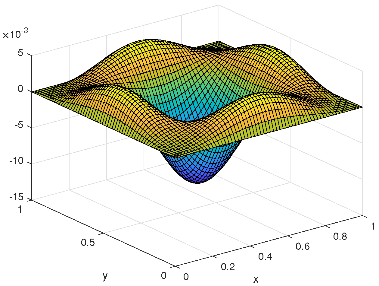
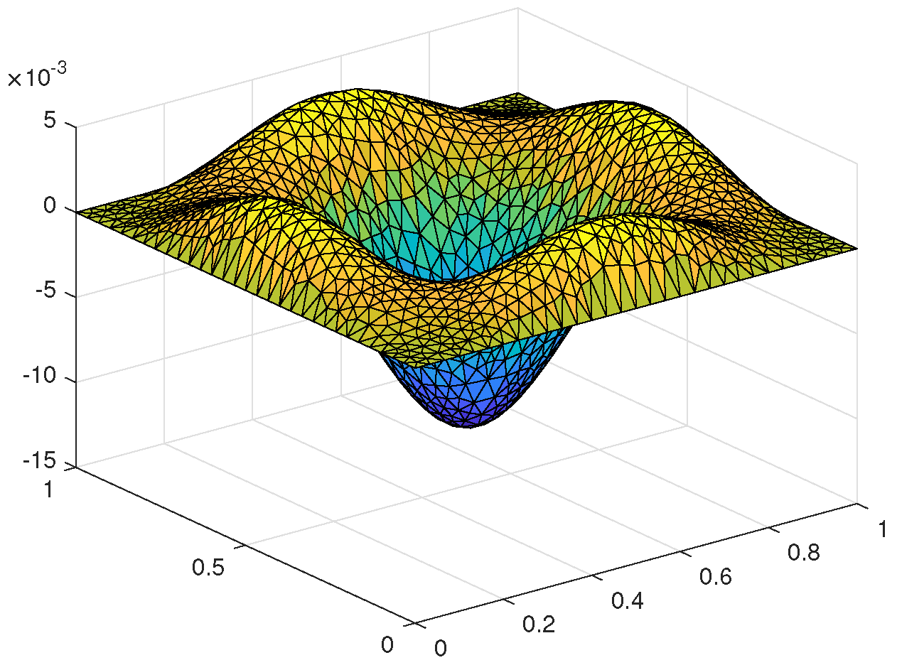
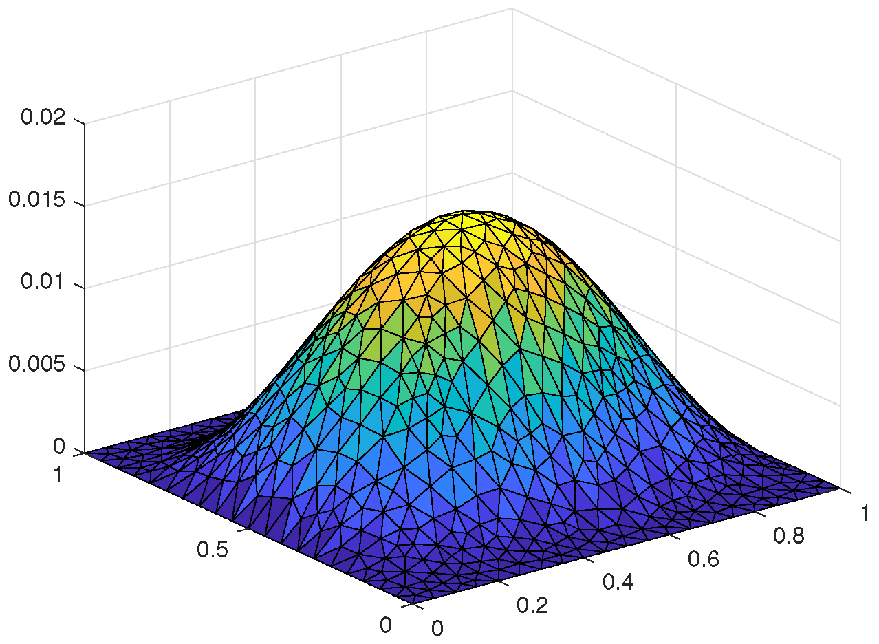
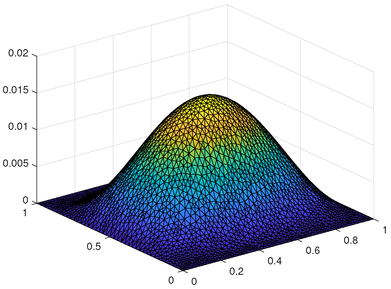
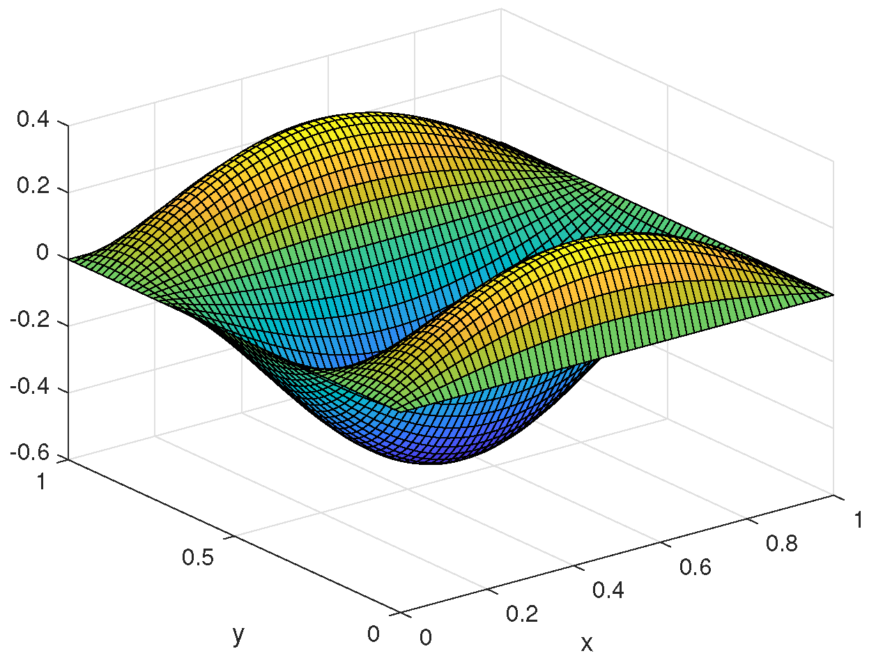
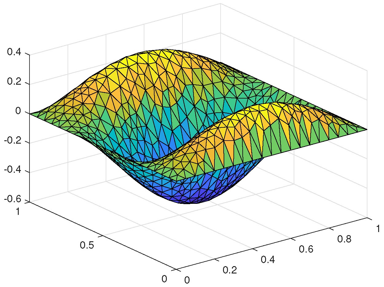
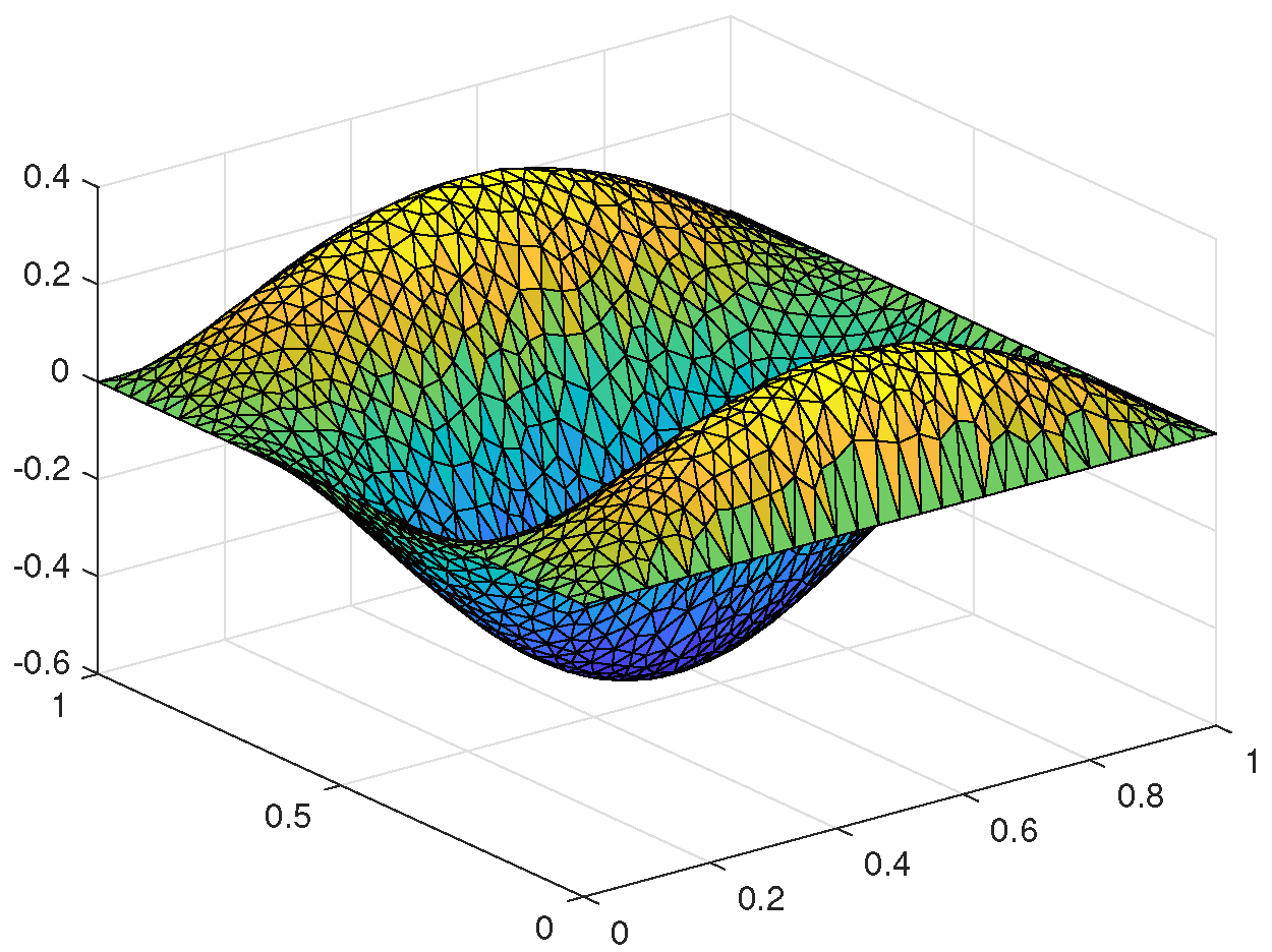
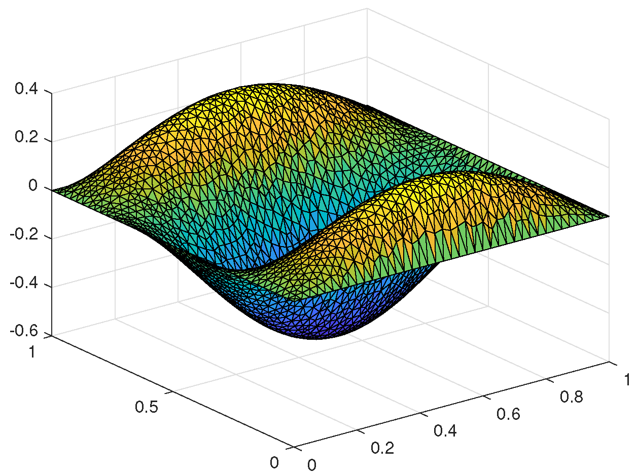
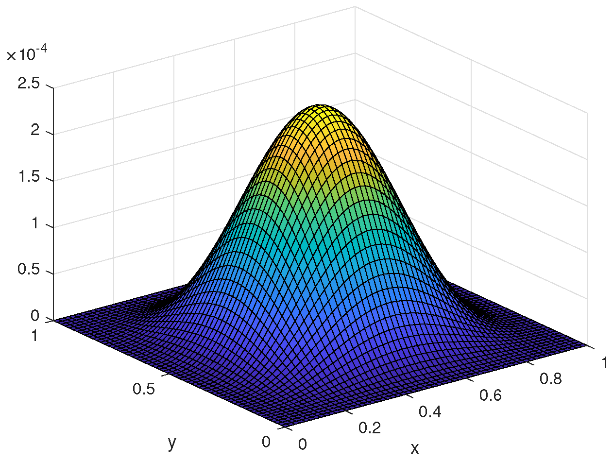
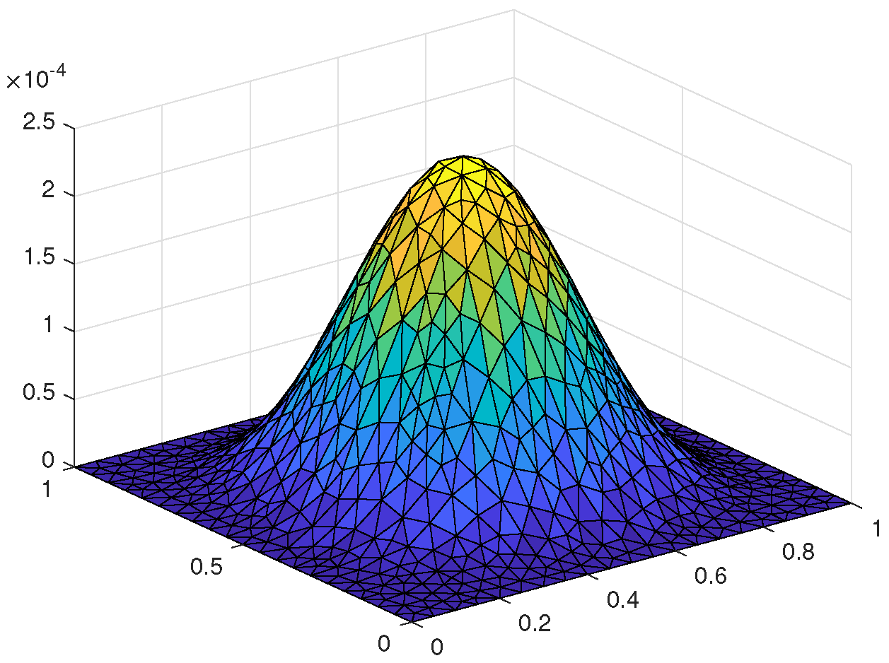
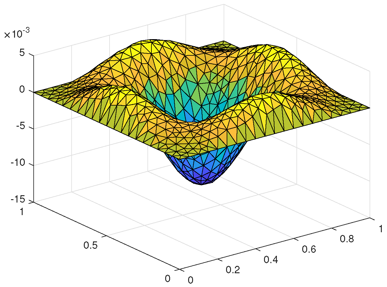
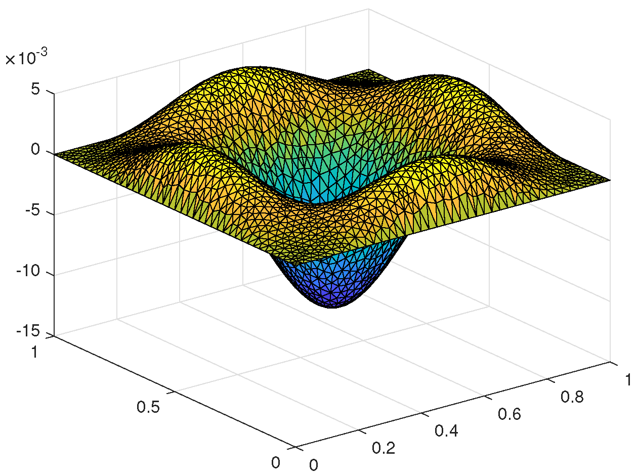
5.1. Two-Dimensional Example Based on the Triangular Meshes

Here, a specific algorithm is given to illustrate how to implement the calculation process, and numerical results are given to verify our theoretical results.

5.1.1. Numerical Algorithm

We show the numerical algorithm with two processes, including the preliminary knowledge of algorithm and the algorithm based on our scheme.

Process I: Preliminary knowledge of the algorithm

We give the numerical algorithm based on the space–time mesh parameters M and N, where N is the number of time cells and M is the number of spatial triangular units.

In order to use linear interpolation in each triangular unit $I_p,(1\le p\le M)$, we take the three vertexes of the unit as interpolation points. If we define the coordinates of three vertexes as $(x_i,y_i)$, $(x_j,y_j)$, $(x_m,y_m)$, the corresponding triangular unit’s area ${\Delta }_e$ can be expressed as a third-order determinant consisting of the coordinates above.

Setting the values of the linear interpolation function $u_h$ at the three nodes $u_i,u_j,u_m$, in triangular unit $I_p$, we can easily work out the three unknown coefficients ${\beta }_1,{\beta }_2,{\beta }_3$ of $u_h$, which are completely determined by $(x_k,y_k)$ and $u_k$, $(k=i,j,m)$.

Further, substituting $\{{\beta }_k,k=1,2,3\}$, into the general form of the linear interpolation function $u_h$, we can obtain the expression for $u_h$ in $I_p$, which is

$$\begin{array}{c}\hfill u_h=N_i{u}_i+N_j{u}_j+N_m{u}_m,\end{array}$$

(31)

where

$$\begin{array}{cc}\hfill N_k(x,y)& =\frac{1}{2{\Delta }_e}(a_{k}x+b_{k}y+c_k),k=i,j,m,\hfill \end{array}$$

(32)

specifically, ${\Delta }_e$ is given as follows, and $a_k,b_k,c_k$ are defined by the latter equation

$$\begin{array}{c}\hfill {\Delta }_e=\frac{1}{2}\left|\begin{array}{ccc}{x}_i& y_i& 1\\ x_j& y_j& 1\\ x_m& y_m& 1\end{array}\right|,h_l=\left|\begin{array}{cc}{s}_{l+1}& r_{l+1}\\ s_{l+2}& r_{l+2}\end{array}\right|,\end{array}$$

(33)

where $h=a,b,c$, and the values of s and r depending on h and the indexes $l+1$ are the following

$$\begin{array}{c}\hfill s=\left\{\begin{array}{c}y,h=a,\hfill \\ -x,h=b,\hfill \\ x,h=c,\hfill \end{array}\right.,r=\left\{\begin{array}{c}1,h=a,b\hfill \\ y,h=c,\hfill \end{array}\right.,l+1=\left\{\begin{array}{c}j,l=i,\hfill \\ m,l=j,\hfill \\ i,l=m,\hfill \end{array}\right.\end{array}$$

(34)

Likewise, the indexes $l+2$ can be obtained by the indexes $l+1$.

Similarly, we set that function v takes $v_i,v_j,v_m$ at mesh nodes $\{i,j,m\}$ in each triangular unit $I_p$. From (31)–(34), we know that

$$\begin{array}{cc}\hfill u_h(x,y)& =\sum _{k=i,j,m}{N}_k(x,y)u_k,v(x,y)=\sum _{k=i,j,m}{N}_k(x,y)v_k,\hfill \\ \hfill \frac{\partial u_h}{\partial x}& =\frac{1}{2{\Delta }_e}\sum _{k=i,j,m}{a}_k{u}_k,\frac{\partial u_h}{\partial y}=\frac{1}{2{\Delta }_e}\sum _{k=i,j,m}{b}_k{u}_k.\hfill \end{array}$$

(35)

To simplify this expression, let us introduce the matrix B and three dimensional column vector ${\mathit{u}}^{\left(e\right)},{\mathit{v}}^{\left(e\right)},{\mathit{w}}^{\left(e\right)},\mathit{N}(x,y)$ as follows

$$\begin{array}{cc}\hfill B=& \frac{1}{2{\Delta }_e}\left[\begin{array}{ccc}{a}_i& a_j& a_m\\ b_i& b_j& b_m\end{array}\right],{\mathit{u}}^{\left(e\right)}={\left[\begin{array}{ccc}{u}_i& u_j& u_m\end{array}\right]}^T,{\mathit{v}}^{\left(e\right)}={\left[\begin{array}{ccc}{v}_i& v_j& v_m\end{array}\right]}^T,\hfill \\ \hfill {\mathit{w}}^{\left(e\right)}=& {\left[\begin{array}{ccc}{w}_i& w_j& w_m\end{array}\right]}^T,\mathit{N}(x,y)={\left[\begin{array}{ccc}{N}_i& N_j& N_m\end{array}\right]}^T.\hfill \end{array}$$

(36)

From (36), the gradients of $u_h(x,y),v(x,y)$ can be expressed as

$$\begin{array}{c}\hfill \nabla u_h=B{\mathit{u}}^{\left(e\right)},\nabla v=B{\mathit{v}}^{\left(e\right)}.\end{array}$$

(37)

Therefore,

$$\begin{array}{c}\hfill u_h(x,y)=\mathit{N}{(x,y)}^T{\mathit{u}}^{\left(e\right)},v(x,y)=\mathit{N}{(x,y)}^T{\mathit{v}}^{\left(e\right)}.\end{array}$$

(38)

Process II: The algorithm based on our scheme

According to the formulas above, we can express (10) and (11) (the case of $n\ge 2$) as

$$\begin{array}{cc}\hfill & ({\left[{\mathit{u}}_{(e)}^n\right]}^T{B}^{T}B,\mathit{v}(e))+({\left[{\sigma }_{(e)}^n\right]}^{T}N{N}^T,\mathit{v}(e))=-((2f({\mathit{u}}^{n-1})-f({\mathit{u}}^{n-2}))N,{\mathit{v}}_{(e)}),\hfill \end{array}$$

(39)

$$\begin{array}{cc}\hfill & (\frac{3}{2\tau }{\left[{\mathit{u}}_{(e)}^n\right]}^{T}N{N}^T,{\mathit{w}}_{(e)})+({\tau }^{\alpha }{\lambda }_0^{(\alpha )}{\left[{\mathit{u}}_{(e)}^n\right]}^T{B}^{T}B,{\mathit{w}}_{(e)})-({\left[{\sigma }_{(e)}^n\right]}^T{B}^{T}B,{\mathit{w}}_{(e)})\hfill \\ \hfill =& (-{\tau }^{\alpha }\sum _{k=1}^n{\lambda }_k^{(\alpha )}{\left[{\mathit{u}}_{(e)}^{n-k}\right]}^T{B}^{T}B,{\mathit{w}}_{(e)})+(\frac{2}{\tau }{\left[{\mathit{u}}_{(e)}^{n-1}\right]}^{T}N{N}^T,{\mathit{w}}_{(e)})\hfill \\ & -(\frac{1}{2\tau }{\left[{\mathit{u}}_{(e)}^{n-2}\right]}^{T}N{N}^T,{\mathit{w}}_{(e)})+(g^n,{\mathit{w}}_{(e)}).\hfill \end{array}$$

(40)

For the case $n=1$ in (11), we can deal with it by a similar method and do not repeat it here. Now, we write (39) and (40) as the following

$$\begin{array}{c}\hfill \sum _e({\left[{\mathit{u}}_{(e)}^n\right]}^T{A}_{(e)}^1{\mathit{v}}_{(e)}+{\left[{\sigma }_{(e)}^n\right]}^T{B}_{(e)}^1{\mathit{v}}_{(e)})=\sum _e{\left[b_{(e)}^1\right]}^T{\mathit{v}}_{(e)},\end{array}$$

(41)

$$\begin{array}{c}\hfill \sum _e({\left[{\mathit{u}}_{(e)}^n\right]}^T{A}_{(e)}^2{\mathit{w}}_{(e)}+{\left[{\sigma }_{(e)}^n\right]}^T{B}_{(e)}^2{\mathit{w}}_{(e)})=\sum _e{\left[b_{(e)}^2\right]}^T{\mathit{w}}_{(e)},\end{array}$$

(42)

where

$$\begin{array}{cc}\hfill A_{(e)}^1& ={\int \int }_e(B^{T}B)\mathrm{d}x\mathrm{d}y,B_{(e)}^1={\int \int }_e(N{N}^T)\mathrm{d}x\mathrm{d}y,\hfill \\ \hfill {\mathit{b}}_{(e)}^1& =-{\int \int }_e(2f({\mathit{u}}^{n-1})-f({\mathit{u}}^{n-2}))N\mathrm{d}x\mathrm{d}y,\hfill \\ \hfill A_{(e)}^2& ={\int \int }_e(\frac{3}{2\tau }N{N}^T+{\tau }^{\alpha }{\lambda }_0^{(\alpha )}{B}^{T}B)\mathrm{d}x\mathrm{d}y,B_{(e)}^2=-{\int \int }_e(B^{T}B)\mathrm{d}x\mathrm{d}y,\hfill \\ \hfill {\mathit{b}}_{(e)}^2& ={\int \int }_e(-{\tau }^{\alpha }\sum _{k=1}^n{\lambda }_k^{(\alpha )}{B}^{T}B{\mathit{u}}_{(e)}^{n-k}+\frac{2}{\tau }N{N}^T{u}_{(e)}^{n-1}-\frac{1}{2\tau }N{N}^T{u}_{(e)}^{n-2}+g^{n}N)\mathrm{d}x\mathrm{d}y.\hfill \end{array}$$

(43)

Clearly, (41) and (42) are equivalent to

$$\begin{array}{c}\hfill \left[\begin{array}{cc}{A}_{\left(e\right)}^1& B_{\left(e\right)}^1\\ A_{\left(e\right)}^2& B_{\left(e\right)}^2\end{array}\right]\left[\begin{array}{c}{\mathit{u}}_{\left(e\right)}^n\\ {\mathit{\sigma }}_{\left(e\right)}^n\end{array}\right]=\left[\begin{array}{c}{\mathit{b}}_{\left(e\right)}^1\\ {\mathit{b}}_{\left(e\right)}^2\end{array}\right].\end{array}$$

(44)

In other words,

$$\begin{array}{c}\hfill K{\overrightarrow{U}}^n={\overrightarrow{G}}^n,1\le n\le N,\end{array}$$

(45)

where

$$\begin{array}{c}\hfill K=\left[\begin{array}{cc}{A}_1& B_1\\ A_2& B_2\end{array}\right],{\overrightarrow{U}}^n=\left[\begin{array}{c}{\mathit{u}}^n\\ {\mathit{\sigma }}^n\end{array}\right],{\overrightarrow{G}}^n=\left[\begin{array}{c}{\mathit{b}}_1^n\\ {\mathit{b}}_2^n\end{array}\right],\end{array}$$

(46)

$$\begin{array}{cc}\hfill A_1=\sum _e{A}_{\left(e\right)}^1,A_2=\sum _e{A}_{\left(e\right)}^2,B_1=\sum _e{B}_{\left(e\right)}^1,B_2=\sum _e{B}_{\left(e\right)}^2,{\mathit{b}}_1^n& =\sum _e{\mathit{b}}_{\left(e\right)}^1,{\mathit{b}}_2^n=\sum _e{\mathit{b}}_{\left(e\right)}^2.\hfill \end{array}$$

(47)

According to (41) and (43), we know that

$$\begin{array}{cc}\hfill A_{\left(e\right)}^1& =\left[\begin{array}{ccccccc}& ⋮& & ⋮& & ⋮& \\ \cdots & a_{ii}^{\left(e\right)}& \cdots & a_{ij}^{\left(e\right)}& \cdots & a_{im}^{\left(e\right)}& \cdots \\ & ⋮& & ⋮& & ⋮& \\ \cdots & a_{ji}^{\left(e\right)}& \cdots & a_{jj}^{\left(e\right)}& \cdots & a_{jm}^{\left(e\right)}& \cdots \\ & ⋮& & ⋮& & ⋮& \\ \cdots & a_{mi}^{\left(e\right)}& \cdots & a_{jm}^{\left(e\right)}& \cdots & a_{mm}^{\left(e\right)}& \cdots \\ & ⋮& & ⋮& & ⋮& \end{array}\right],B_{\left(e\right)}^1=\left[\begin{array}{ccccccc}& ⋮& & ⋮& & ⋮& \\ \cdots & b_{ii}^{\left(e\right)}& \cdots & b_{ij}^{\left(e\right)}& \cdots & b_{im}^{\left(e\right)}& \cdots \\ & ⋮& & ⋮& & ⋮& \\ \cdots & b_{ji}^{\left(e\right)}& \cdots & b_{jj}^{\left(e\right)}& \cdots & b_{jm}^{\left(e\right)}& \cdots \\ & ⋮& & ⋮& & ⋮& \\ \cdots & b_{mi}^{\left(e\right)}& \cdots & b_{jm}^{\left(e\right)}& \cdots & b_{mm}^{\left(e\right)}& \cdots \\ & ⋮& & ⋮& & ⋮& \end{array}\right],\hfill \end{array}$$

$$\begin{array}{cc}\hfill A_{\left(e\right)}^2& =\left[\begin{array}{ccccccc}& ⋮& & ⋮& & ⋮& \\ \cdots & c_{ii}^{\left(e\right)}& \cdots & c_{ij}^{\left(e\right)}& \cdots & c_{im}^{\left(e\right)}& \cdots \\ & ⋮& & ⋮& & ⋮& \\ \cdots & c_{ji}^{\left(e\right)}& \cdots & c_{jj}^{\left(e\right)}& \cdots & c_{jm}^{\left(e\right)}& \cdots \\ & ⋮& & ⋮& & ⋮& \\ \cdots & c_{mi}^{\left(e\right)}& \cdots & c_{jm}^{\left(e\right)}& \cdots & c_{mm}^{\left(e\right)}& \cdots \\ & ⋮& & ⋮& & ⋮& \end{array}\right],B_{\left(e\right)}^2=\left[\begin{array}{ccccccc}& ⋮& & ⋮& & ⋮& \\ \cdots & d_{ii}^{\left(e\right)}& \cdots & d_{ij}^{\left(e\right)}& \cdots & d_{im}^{\left(e\right)}& \cdots \\ & ⋮& & ⋮& & ⋮& \\ \cdots & d_{ji}^{\left(e\right)}& \cdots & d_{jj}^{\left(e\right)}& \cdots & d_{jm}^{\left(e\right)}& \cdots \\ & ⋮& & ⋮& & ⋮& \\ \cdots & b_{mi}^{\left(e\right)}& \cdots & d_{jm}^{\left(e\right)}& \cdots & d_{mm}^{\left(e\right)}& \cdots \\ & ⋮& & ⋮& & ⋮& \end{array}\right],\hfill \end{array}$$

$$\begin{array}{cc}\hfill {\mathit{b}}_{\left(e\right)}^1& ={\left[\begin{array}{ccccccc}\cdots & b_{i1}^{\left(e\right)}& \cdots & b_{j1}^{\left(e\right)}& \cdots & b_{m1}^{\left(e\right)}& \cdots \end{array}\right]}^T,{\mathit{b}}_{\left(e\right)}^2={\left[\begin{array}{ccccccc}\cdots & b_{i2}^{\left(e\right)}& \cdots & b_{j2}^{\left(e\right)}& \cdots & b_{m2}^{\left(e\right)}& \cdots \end{array}\right]}^T,\hfill \end{array}$$

and

$$\begin{array}{cc}\hfill a_{kl}^{(e)}=& {\int \int }_e\frac{1}{4{\Delta }_e^2}(a_k{a}_l+b_k{b}_l)\mathrm{d}x\mathrm{d}y,b_{kl}^{(e)}={\int \int }_e{N}_k{N}_l\mathrm{d}x\mathrm{d}y,(k,l=i,j,m),\hfill \\ \hfill c_{kl}^{(e)}=& {\int \int }_e(\frac{3}{2\tau }{N}_k{N}_l+{\tau }^{\alpha }{\lambda }_0\frac{1}{4{\Delta }_e^2}(a_k{a}_l+b_k{b}_l))\mathrm{d}x\mathrm{d}y,d_{kl}^{(e)}={\int \int }_e-\frac{1}{4{\Delta }_e^2}(a_k{a}_l+b_k{b}_l)\mathrm{d}x\mathrm{d}y,\hfill \\ \hfill b_{1i}^{(e)}=& {\int \int }_e-(2f(u_e^{n-1})-f(u_e^{n-2}))N_i\mathrm{d}x\mathrm{d}y,\hfill \\ \hfill b_{1j}^{(e)}=& {\int \int }_e-(2f(u_e^{n-1})-f(u_e^{n-2}))N_j\mathrm{d}x\mathrm{d}y,\hfill \\ \hfill b_{1m}^{(e)}=& {\int \int }_e-(2f(u_e^{n-1})-f(u_e^{n-2}))N_m\mathrm{d}x\mathrm{d}y,\hfill \\ \hfill b_{2i}^{(e)}=& {\int \int }_e(-{\tau }^{\alpha }\frac{1}{4{\Delta }_e^2}\sum _{k=1}^n{\lambda }_k^{\alpha }((a_i^2+b_i^2)u_{e,i}^{n-k}+(a_i{a}_j+b_i{b}_j)u_{e,j}^{n-k}+(a_i{a}_m+b_i{b}_m)u_{e,m}^{n-k})\hfill \\ \hfill & +\frac{2}{\tau }(N_i{N}_i{u}_{e,i}^{n-1}+N_i{N}_j{u}_{e,j}^{n-1}+N_i{N}_m{u}_{e,m}^{n-1})\hfill \\ \hfill & -\frac{1}{2\tau }(N_i{N}_i{u}_{e,i}^{n-2}+N_i{N}_j{u}_{e,j}^{n-2}+N_i{N}_m{u}_{e,m}^{n-2})+g^n{N}_i)\mathrm{d}x\mathrm{d}y,\hfill \\ \hfill b_{2j}^{(e)}=& {\int \int }_e(-{\tau }^{\alpha }\frac{1}{4{\Delta }_e^2}\sum _{k=1}^n{\lambda }_k^{\alpha }((a_i{a}_j+b_i{b}_j)u_{e,i}^{n-k}+(a_j^2+b_j^2)u_{e,j}^{n-k}+(a_j{a}_m+b_j{b}_m)u_{e,m}^{n-k})\hfill \\ \hfill & +\frac{2}{\tau }(N_i{N}_j{u}_{e,i}^{n-1}+N_j{N}_j{u}_{e,j}^{n-1}+N_j{N}_m{u}_{e,m}^{n-1})\hfill \\ \hfill & -\frac{1}{2\tau }(N_i{N}_j{u}_{e,i}^{n-2}+N_j{N}_j{u}_{e,j}^{n-2}+N_j{N}_m{u}_{e,m}^{n-2})+g^n{N}_j)\mathrm{d}x\mathrm{d}y,\hfill \\ \hfill b_{2m}^{(e)}=& {\int \int }_e(-{\tau }^{\alpha }\frac{1}{4{\Delta }_e^2}\sum _{k=1}^n{\lambda }_k^{\alpha }((a_i{a}_m+b_i{b}_m)u_{e,i}^{n-k}+(a_j{a}_m+b_j{b}_m)u_{e,j}^{n-k}+(a_m^2+b_m^2)u_{e,m}^{n-k})\hfill \\ \hfill & +\frac{2}{\tau }(N_i{N}_m{u}_{e,i}^{n-1}+N_j{N}_m{u}_{e,j}^{n-1}+N_m{N}_m{u}_{e,m}^{n-1})\hfill \\ \hfill & -\frac{1}{2\tau }(N_i{N}_m{u}_{e,i}^{n-2}+N_j{N}_m{u}_{e,j}^{n-2}+N_m{N}_m{u}_{e,m}^{n-2})+g^n{N}_m)\mathrm{d}x\mathrm{d}y.\hfill \end{array}$$

(48)

Based on system (45), we can obtain the unique numerical solution of u and $\sigma$.

5.1.2. Numerical Calculations

For reflecting the effectiveness of the considered numerical method in the current article, two numerical examples with initial and boundary conditions are provided. In these tests, we take $z=(x,y)\in \mathrm{\Omega }=(0,1)\times (0,1)$ and $T=1$.

Example 1.

We take the exact solution of (1) as $u(x,y,t)=t^3(sin\pi x)y^3{\left(1-y\right)}^3$ and then substitute it into (2) to find

$$\begin{array}{c}\hfill {}_0{\mathcal{I}}_t^{\alpha }u=\frac{6(sin\pi x)y^3{\left(1-y\right)}^3}{\mathrm{\Gamma }(\alpha +4)}{t}^{\alpha +3}.\end{array}$$

(49)

Now, we take the nonlinear term $f\left(u\right)=sinu$ and obtain the corresponding source term $g(x,y,t)$. Here, we show the effectiveness by the calculated data in

Table 1. The spatial convergence results for u and $\sigma$ with $\tau =\frac{1}{200}$.

$\mathit{\alpha }$	h	${\mathit{E}}_{\mathit{u}}(\mathit{\tau },\mathit{h})$	Rate	${\mathit{E}}_{\mathit{\sigma }}(\mathit{\tau },\mathit{h})$	Rate
0.1	1/4	1.2160 × 10${}^{-3}$	—	7.3073 × 10${}^{-2}$	—
	1/8	3.0300 × 10${}^{-4}$	2.0047	1.8151 × 10${}^{-2}$	2.0093
	1/16	7.5223 × 10${}^{-5}$	2.0101	4.7932 × 10${}^{-3}$	1.9210
	1/32	1.8735 × 10${}^{-5}$	2.0054	1.1330 × 10${}^{-3}$	2.0809
0.3	1/4	1.2189 × 10${}^{-3}$	—	7.3130 × 10${}^{-2}$	—
	1/8	3.0367 × 10${}^{-4}$	2.0050	1.8170 × 10${}^{-2}$	2.0089
	1/16	7.5369 × 10${}^{-5}$	2.0104	4.7981 × 10${}^{-3}$	1.9210
	1/32	1.8771 × 10${}^{-5}$	2.0055	1.1342 × 10${}^{-3}$	2.0807
0.5	1/4	1.2212 × 10${}^{-3}$	—	7.3175 × 10${}^{-2}$	—
	1/8	3.0420 × 10${}^{-4}$	2.0052	1.8185 × 10${}^{-2}$	2.0086
	1/16	7.5486 × 10${}^{-5}$	2.0107	4.8020 × 10${}^{-3}$	1.9210
	1/32	1.8799 × 10${}^{-5}$	2.0055	1.1353 × 10${}^{-3}$	2.0806
0.7	1/4	1.2230 × 10${}^{-3}$	—	7.3210 × 10${}^{-2}$	—
	1/8	3.0463 × 10${}^{-4}$	2.0054	1.8197 × 10${}^{-2}$	2.0084
	1/16	7.5579 × 10${}^{-5}$	2.0110	4.8052 × 10${}^{-3}$	1.9210
	1/32	1.8821 × 10${}^{-5}$	2.0056	1.1361 × 10${}^{-3}$	2.0806
0.9	1/4	1.2245 × 10${}^{-3}$	—	7.3238 × 10${}^{-2}$	—
	1/8	3.0496 × 10${}^{-4}$	2.0055	1.8206 × 10${}^{-2}$	2.0082
	1/16	7.5651 × 10${}^{-5}$	2.0112	4.8076 × 10${}^{-3}$	1.9210
	1/32	1.8839 × 10${}^{-5}$	2.0057	1.1367 × 10${}^{-3}$	2.0805

and

Table 2. The space–time convergence results for u and $\sigma$.

$\mathit{\alpha }$	$(\mathit{\tau },\mathit{h})$	${\mathit{E}}_{\mathit{u}}(\mathit{\tau },\mathit{h})$	Rate	${\mathit{E}}_{\mathit{\sigma }}(\mathit{\tau },\mathit{h})$	Rate
0.1	(1/10,1/10)	2.0896 × 10${}^{-4}$	—	1.3569 × 10${}^{-2}$	—
	(1/20,1/20)	4.6046 × 10${}^{-5}$	2.1821	3.0399 × 10${}^{-3}$	2.1582
	(1/30,1/30)	2.0672 × 10${}^{-5}$	1.9751	1.3515 × 10${}^{-3}$	1.9993
	(1/40,1/40)	1.1502 × 10${}^{-5}$	2.0381	7.4700 × 10${}^{-4}$	2.0609
0.3	(1/10,1/10)	2.0955 × 10${}^{-4}$	—	1.3585 × 10${}^{-2}$	—
	(1/20,1/20)	4.6178 × 10${}^{-5}$	2.1820	3.0437 × 10${}^{-3}$	2.1582
	(1/30,1/30)	2.0731 × 10${}^{-5}$	1.9753	1.3532 × 10${}^{-3}$	1.9992
	(1/40,1/40)	1.1535 × 10${}^{-5}$	2.0377	7.4796 × 10${}^{-4}$	2.0609
0.5	(1/10,1/10)	2.0995 × 10${}^{-4}$	—	1.3597 × 10${}^{-2}$	—
	(1/20,1/20)	4.6263 × 10${}^{-5}$	2.1821	3.0465 × 10${}^{-3}$	2.1581
	(1/30,1/30)	2.0768 × 10${}^{-5}$	1.9754	1.3545 × 10${}^{-3}$	1.9991
	(1/40,1/40)	1.1557 × 10${}^{-5}$	2.0374	7.4866 × 10${}^{-4}$	2.0609
0.7	(1/10,1/10)	2.1018 × 10${}^{-4}$	—	1.3606 × 10${}^{-2}$	—
	(1/20,1/20)	4.6309 × 10${}^{-5}$	2.1822	3.0484 × 10${}^{-3}$	2.1581
	(1/30,1/30)	2.0788 × 10${}^{-5}$	1.9754	1.3554 × 10${}^{-3}$	1.9990
	(1/40,1/40)	1.1568 × 10${}^{-5}$	2.0373	7.4916 × 10${}^{-4}$	2.0609
0.9	(1/10,1/10)	2.1028 × 10${}^{-4}$	—	1.3612 × 10${}^{-2}$	—
	(1/20,1/20)	4.6327 × 10${}^{-5}$	2.1824	3.0498 × 10${}^{-3}$	2.1581
	(1/30,1/30)	2.0795 × 10${}^{-5}$	1.9755	1.3560 × 10${}^{-3}$	1.9990
	(1/40,1/40)	1.1573 × 10${}^{-5}$	2.0373	7.4950 × 10${}^{-4}$	2.0609

.

For the fractional parameters $\alpha =0.1,0.3,0.5,0.7,0.9$, we fix the time step length parameter $\tau =1/200$ and change the spatial grid parameters $h=1/4,1/8,1/16,1/32$ to arrive at the spatial convergence results for both u and $\sigma$ in Table 1. Further, by taking $(\tau ,h)=(\frac{1}{10},\frac{1}{10}),(\frac{1}{20},\frac{1}{20}),(\frac{1}{30},\frac{1}{30}),(\frac{1}{40},\frac{1}{40})$, we calculate the space–time convergence results shown in Table 2. The computed data illustrate that we can arrive at the approximating second-order convergence rate, which is in agreement with our theory results. In Figure 1, Figure 2, Figure 3 and Figure 4, we show the approximate process between $u_h$ and u by taking the fractional parameter $\alpha =0.1$ and space–time step length parameters $\tau =h=1/20$, $1/30$ and $1/40$. We also show the approximation behavior between ${\sigma }_h$ and $\sigma$ in Figure 5, Figure 6, Figure 7 and Figure 8.

Example 2.

Now, we consider another numerical example to further validate the convergence for our method. We take the exact solution $u(x,y,t)=t^{2.5}{x}^3{\left(1-x\right)}^3{y}^3{\left(1-y\right)}^3$ and then obtain

$$\begin{array}{c}\hfill {}_0{\mathcal{I}}_t^{\alpha }u=\frac{\mathrm{\Gamma }\left(3.5\right)}{\mathrm{\Gamma }(\alpha +3.5)}{x}^3{\left(1-x\right)}^3{y}^3{\left(1-y\right)}^3{t}^{\alpha +2.5}.\end{array}$$

(50)

Next, we choose the nonlinear term $f\left(u\right)=u^3-u$ to obtain the corresponding source term $g(x,y,t)$. In this case, we continue to do our tests.

Here, we list the computing data including errors and convergence orders in

Table 3. The spatial convergence results for u and $\sigma$ with $\tau =\frac{1}{200}$.

$\mathit{\alpha }$	h	${\mathit{E}}_{\mathit{u}}(\mathit{\tau },\mathit{h})$	Rate	${\mathit{E}}_{\mathit{\sigma }}(\mathit{\tau },\mathit{h})$	Rate
0.1	1/4	1.9466 × 10${}^{-5}$	—	1.4787 × 10${}^{-3}$	—
	1/8	4.8028 × 10${}^{-6}$	2.0190	3.2835 × 10${}^{-4}$	2.1711
	1/16	1.2213 × 10${}^{-6}$	1.9755	8.8243 × 10${}^{-5}$	1.8957
	1/32	3.1213 × 10${}^{-7}$	1.9682	2.1371 × 10${}^{-5}$	2.0458
0.3	1/4	1.9495 × 10${}^{-5}$	—	1.4795 × 10${}^{-3}$	—
	1/8	4.8101 × 10${}^{-6}$	2.0190	3.2864 × 10${}^{-4}$	2.1705
	1/16	1.2229 × 10${}^{-6}$	1.9758	8.8322 × 10${}^{-5}$	1.8957
	1/32	3.1254 × 10${}^{-7}$	1.9682	2.1392 × 10${}^{-5}$	2.0457
0.5	1/4	1.9520 × 10${}^{-5}$	—	1.4801 × 10${}^{-3}$	—
	1/8	4.8163 × 10${}^{-6}$	2.0190	3.2889 × 10${}^{-4}$	2.1701
	1/16	1.2242 × 10${}^{-6}$	1.9760	8.8388 × 10${}^{-5}$	1.8957
	1/32	3.1289 × 10${}^{-7}$	1.9681	2.1409 × 10${}^{-5}$	2.0456
0.7	1/4	1.9541 × 10${}^{-5}$	—	1.4806 × 10${}^{-3}$	—
	1/8	4.8213 × 10${}^{-6}$	2.0190	3.2909 × 10${}^{-4}$	2.1697
	1/16	1.2253 × 10${}^{-6}$	1.9763	8.8442 × 10${}^{-5}$	1.8957
	1/32	3.1317 × 10${}^{-7}$	1.9681	2.1423 × 10${}^{-5}$	2.0456
0.9	1/4	1.9557 × 10${}^{-5}$	—	1.4811 × 10${}^{-3}$	—
	1/8	4.8254 × 10${}^{-6}$	2.0190	3.2925 × 10${}^{-4}$	2.1694
	1/16	1.2262 × 10${}^{-6}$	1.9764	8.8485 × 10${}^{-5}$	1.8957
	1/32	3.1340 × 10${}^{-7}$	1.9681	2.1434 × 10${}^{-5}$	2.0455

and

Table 4. The space–time convergence results for u and $\sigma$.

$\mathit{\alpha }$	$(\mathit{\tau },\mathit{h})$	${\mathit{E}}_{\mathit{u}}(\mathit{\tau },\mathit{h})$	Rate	${\mathit{E}}_{\mathit{\sigma }}(\mathit{\tau },\mathit{h})$	Rate
0.1	(1/10,1/10)	3.6207 × 10${}^{-6}$	—	2.5835 × 10${}^{-4}$	—
	(1/20,1/20)	8.4923 × 10${}^{-7}$	2.0920	5.9985 × 10${}^{-5}$	2.1066
	(1/30,1/30)	3.7741 × 10${}^{-7}$	2.0002	2.6440 × 10${}^{-5}$	2.0204
	(1/40,1/40)	2.0890 × 10${}^{-7}$	2.0561	1.4528 × 10${}^{-5}$	2.0816
0.3	(1/10,1/10)	3.6281 × 10${}^{-6}$	—	2.5859 × 10${}^{-4}$	—
	(1/20,1/20)	8.5093 × 10${}^{-7}$	2.0921	6.0046 × 10${}^{-5}$	2.1065
	(1/30,1/30)	3.7812 × 10${}^{-7}$	2.0005	2.6468 × 10${}^{-5}$	2.0203
	(1/40,1/40)	2.0931 × 10${}^{-7}$	2.0556	1.4543 × 10${}^{-5}$	2.0816
0.5	(1/10,1/10)	3.6338 × 10${}^{-6}$	—	2.5879 × 10${}^{-4}$	—
	(1/20,1/20)	8.5222 × 10${}^{-7}$	2.0922	6.0095 × 10${}^{-5}$	2.1065
	(1/30,1/30)	3.7865 × 10${}^{-7}$	2.0008	2.6490 × 10${}^{-5}$	2.0203
	(1/40,1/40)	2.0963 × 10${}^{-7}$	2.0553	1.4555 × 10${}^{-5}$	2.0816
0.7	(1/10,1/10)	3.6379 × 10${}^{-6}$	—	2.5894 × 10${}^{-4}$	—
	(1/20,1/20)	8.5315 × 10${}^{-7}$	2.0923	6.0133 × 10${}^{-5}$	2.1064
	(1/30,1/30)	3.7903 × 10${}^{-7}$	2.0010	2.6508 × 10${}^{-5}$	2.0202
	(1/40,1/40)	2.0986 × 10${}^{-7}$	2.0550	1.4565 × 10${}^{-5}$	2.0816
0.9	(1/10,1/10)	3.6407 × 10${}^{-6}$	—	2.5905 × 10${}^{-4}$	—
	(1/20,1/20)	8.5375 × 10${}^{-7}$	2.0923	6.0162 × 10${}^{-5}$	2.1063
	(1/30,1/30)	3.7927 × 10${}^{-7}$	2.0011	2.6521 × 10${}^{-5}$	2.0202
	(1/40,1/40)	2.1000 × 10${}^{-7}$	2.0549	1.4572 × 10${}^{-5}$	2.0816

and the approximation behaviors between the numerical solution and the exact solution in Figure 9, Figure 10, Figure 11 and Figure 12 with the chosen same fractional parameter $\alpha$ and space–time step length sizes to the ones used in Example 1. From Table 3 and Table 4 and Figure 13, Figure 14, Figure 15 and Figure 16, it is easy to see that the approximation effect is consistent with the theoretical results.

To further show the advantages of our method, we need to make a comparison with other numerical schemes. Now, we compute the Example 2 by using another method presented in Remark 1 and obtain the numerical results shown in

Table 5. The spatial convergence rate for u and $\sigma$ with $\tau =\frac{1}{200}$.

$\mathit{\alpha }$	h	${\mathit{E}}_{\mathit{u}}(\mathit{\tau },\mathit{h})$	Rate	${\mathit{E}}_{\mathit{\sigma }}(\mathit{\tau },\mathit{h})$	Rate
0.1	1/4	2.5596 × 10${}^{-5}$	—	1.8764 × 10${}^{-3}$	—
	1/8	5.6306 × 10${}^{-6}$	2.1845	4.2919 × 10${}^{-4}$	2.1283
	1/16	1.4004 × 10${}^{-6}$	2.0075	1.0788 × 10${}^{-4}$	1.9922
	1/32	3.5652 × 10${}^{-7}$	1.9738	2.7133 × 10${}^{-5}$	1.9913
0.3	1/4	2.5633 × 10${}^{-5}$	—	1.8737 × 10${}^{-3}$	—
	1/8	5.6380 × 10${}^{-6}$	2.1847	4.2868 × 10${}^{-4}$	2.1279
	1/16	1.4020 × 10${}^{-6}$	2.0077	1.0776 × 10${}^{-4}$	1.9921
	1/32	3.5693 × 10${}^{-7}$	1.9738	2.7104 × 10${}^{-5}$	1.9913
0.5	1/4	2.5664 × 10${}^{-5}$	—	1.8714 × 10${}^{-3}$	—
	1/8	5.6443 × 10${}^{-6}$	2.1849	4.2826 × 10${}^{-4}$	2.1275
	1/16	1.4033 × 10${}^{-6}$	2.0079	1.0766 × 10${}^{-4}$	1.9920
	1/32	3.5727 × 10${}^{-7}$	1.9738	2.7079 × 10${}^{-5}$	1.9913
0.7	1/4	2.5689 × 10${}^{-5}$	—	1.8695 × 10${}^{-3}$	—
	1/8	5.6494 × 10${}^{-6}$	2.1850	4.2792 × 10${}^{-4}$	2.1272
	1/16	1.4044 × 10${}^{-6}$	2.0081	1.0758 × 10${}^{-4}$	1.9919
	1/32	3.5755 × 10${}^{-7}$	1.9738	2.7059 × 10${}^{-5}$	1.9912
0.9	1/4	2.5710 × 10${}^{-5}$	—	1.8680 × 10${}^{-3}$	—
	1/8	5.6535 × 10${}^{-6}$	2.1851	4.2765 × 10${}^{-4}$	2.1270
	1/16	1.4053 × 10${}^{-6}$	2.0083	1.0752 × 10${}^{-4}$	1.9919
	1/32	3.5777 × 10${}^{-7}$	1.9738	2.7043 × 10${}^{-5}$	1.9912

. By the comparison of errors $E_u(\tau ,h)$ and $E_{\sigma }(\tau ,h)$ between Table 3 and Table 5, one easily finds that our method can obtain the better calculation accuracy.

6. Conclusions

In this article, we developed a fully discrete mixed element system with a second-order time stepping scheme to numerically solve 2D nonlinear fourth-order fractional integral equations. By computing numerical data, including errors and convergence orders, we found that the proposed fully discrete mixed element system was feasible.

References

1. Abbaszadeh, M.; Dehghan, M. Direct meshless local Petrov-Galerkin (DMLPG) method for time-fractional fourth-order reaction-diffusion problem on complex domains. Comput. Math. Appl. 2020, 79, 876–888. [Google Scholar] [CrossRef]
2. Liu, Y.; Du, Y.W.; Li, H.; Li, J.C.; He, S. A two-grid mixed finite element method for a nonlinear fourth-order reaction-diffusion problem with time-fractional derivative. Comput. Math. Appl. 2015, 70, 2474–2492. [Google Scholar] [CrossRef]
3. Nikan, O.; Machado, J.A.T.; Golbabai, A. Numerical solution of time-fractional fourth-order reaction-diffusion model arising in composite environments. Appl. Math. Model. 2021, 89, 819–836. [Google Scholar] [CrossRef]
4. Ji, C.C.; Sun, Z.Z.; Hao, Z.P. Numerical algorithms with high spatial accuracy for the fourth-order fractional sub-diffusion equations with the first Dirichlet boundary conditions. J. Sci. Comput. 2016, 66, 1148–1174. [Google Scholar] [CrossRef]
5. Haghi, M.; Ilati, M.; Dehghan, M. A fourth-order compact difference method for the nonlinear time-fractional fourth-order reaction-diffusion equation. Eng. Comput. 2021, 1–12. [Google Scholar] [CrossRef]
6. Wang, J.R.; Liu, Y.; Wen, C.; Li, H. Efficient numerical algorithm with the second-order time accuracy for a two-dimensional nonlinear fourth-order fractional wave equation. Results Appl. Math. 2022. [Google Scholar]
7. Li, X.H.; Wong, P.J.Y. A non-polynomial numerical scheme for fourth-order fractional diffusion-wave model. Appl. Math. Comput. 2018, 331, 80–95. [Google Scholar] [CrossRef]
8. Akram, G.; Abbas, M.; Tariq, H.; Sadaf, M.; Abdeljawad, T.; Alqudah, M.A. Numerical approximations for the solutions of fourth order time fractional evolution problems using a novel spline technique. Fractal Fract. 2022, 6, 170. [Google Scholar] [CrossRef]
9. Fakhar-Izadi, F.; Shabgard, N. Time-space spectral Galerkin method for time-fractional fourth-order partial differential equations. J. Appl. Math. Comput. 2022, 1–20. [Google Scholar] [CrossRef]
10. Arshad, S.; Wali, M.; Huang, J.F.; Khalid, S.; Akbar, N. Numerical framework for the Caputo time-fractional diffusion equation with fourth order derivative in space. J. Appl. Math. Comput. 2021, 1–22. [Google Scholar] [CrossRef]
11. Nandal, S.; Pandey, D.N. Numerical technique for fractional variable-order differential equation of fourth-order with delay. Appl. Numer. Math. 2021, 161, 391–407. [Google Scholar] [CrossRef]
12. Ran, M.H.; Zhang, C.J. New compact difference scheme for solving the fourth-order time fractional sub-diffusion equation of the distributed order. Appl. Numer. Math. 2018, 129, 58–70. [Google Scholar] [CrossRef]
13. Nawaz, Y. Variational iteration method and homotopy perturbation method for fourth-order fractional integro-differential equations. Comput. Math. Appl. 2011, 61, 2330–2341. [Google Scholar] [CrossRef] [Green Version]
14. Yang, X.H.; Xu, D.; Zhang, H.X. Crank-Nicolson/quasi-wavelets method for solving fourth order partial integro-differential equation with a weakly singular kernel. J. Comput. Phys. 2013, 234, 317–329. [Google Scholar] [CrossRef]
15. Liu, Y.L.; Yang, X.H.; Zhang, H.X.; Liu, Y. Analysis of BDF2 finite difference method for fourth-order integro-differential equation. Comput. Appl. Math. 2021, 40, 57. [Google Scholar] [CrossRef]
16. Qiu, W.L.; Xu, D.; Guo, J. Numerical solution of the fourth-order partial integro-differential equation with multi-term kernels by the Sinc-collocation method based on the double exponential transformation. Appl. Math. Comput. 2021, 392, 125693. [Google Scholar] [CrossRef]
17. Wang, Z.B.; Vong, S. Compact difference schemes for the modified anomalous fractional sub-diffusion equation and the fractional diffusion-wave equation. J. Comput. Phys. 2014, 277, 1–15. [Google Scholar] [CrossRef] [Green Version]
18. Tian, W.Y.; Zhou, H.; Deng, W.H. A class of second order difference approximations for solving space fractional diffusion equations. Math. Comput. 2015, 84, 1703–1727. [Google Scholar] [CrossRef] [Green Version]
19. Feng, R.H.; Liu, Y.; Hou, Y.X.; Li, H.; Fang, Z.C. Mixed element algorithm based on a second-order time approximation scheme for a two-dimensional nonlinear time fractional coupled sub-diffusion model. Eng. Comput. 2022, 38, 51–68. [Google Scholar] [CrossRef]
20. Cao, Y.; Yin, B.L.; Liu, Y.; Li, H. Crank-Nicolson WSGI difference scheme with finite element method for multi-dimensional time-fractional wave problem. Comput. Appl. Math. 2018, 37, 5126–5145. [Google Scholar] [CrossRef]
Figure 1. Exact solution u at t = 1 .
Fractalfract 06 00201 g001
Figure 2. u h with τ = h = 1 20 .
Fractalfract 06 00201 g002
Figure 3. u h with τ = h = 1 30 .
Fractalfract 06 00201 g003
Figure 4. u h with τ = h = 1 40 .
Fractalfract 06 00201 g004
Figure 5. Exact solution σ at t = 1 .
Fractalfract 06 00201 g005
Figure 6. σ h with τ = h = 1 20 .
Fractalfract 06 00201 g006
Figure 7. σ h with τ = h = 1 30 .
Fractalfract 06 00201 g007
Figure 8. σ h with τ = h = 1 40 .
Fractalfract 06 00201 g008
Figure 9. Exact solution u at t = 1 .
Fractalfract 06 00201 g009
Figure 10. u h with τ = h = 1 20 .
Fractalfract 06 00201 g010
Figure 11. u h with τ = h = 1 30 .
Fractalfract 06 00201 g011
Figure 12. u h with τ = h = 1 40 .
Fractalfract 06 00201 g012
Figure 13. Exact solution σ at t = 1 .
Fractalfract 06 00201 g013
Figure 14. σ h with τ = h = 1 20 .
Fractalfract 06 00201 g014
Figure 15. σ h with τ = h = 1 30 .
Fractalfract 06 00201 g015
Figure 16. σ h with τ = h = 1 40 .
Fractalfract 06 00201 g016