Modified Predictor–Corrector Method for the Numerical Solution of a Fractional-Order SIR Model with 2019-nCoV

Abstract

In this paper, we analyzed and found the solution for a suitable nonlinear fractional dynamical system that describes coronavirus (2019-nCoV) using a novel computational method. A compartmental model with four compartments, namely, susceptible, infected, reported and unreported, was adopted and modified to a new model incorporating fractional operators. In particular, by using a modified predictor–corrector method, we captured the nature of the obtained solution for different arbitrary orders. We investigated the influence of the fractional operator to present and discuss some interesting properties of the novel coronavirus infection.

1. Introduction

Due to 2019-nCOV, more than 11 billion people have been infected, 535,108 people have died and 6,491,870 people have recovered around the globe as of 5 July 2021 [1,2,3]. The investigation of the evolution of the novel coronavirus and predication of the corresponding consequences plays a vital role in the investigation of diseases and the study of epidemic models. These phenomena can be efficiently studied by several suitable differential models. However, when we want to incorporate some memory-based consequences, the concept of classical calculus fails to explain the properties. In this regard, many phenomena associated with complexity and high nonlinearity are accurately and effectively described by fractional calculus (FC) [4,5,6,7,8,9,10,11,12,13,14].

Many researchers have studied and derived some essential and important results with respect to behavior, evolution, character and other critical objectives concerning coronavirus. For instance, in [15], the authors presented some interesting consequences of coronavirus infection and the interaction between unknown hosts and bats. Phase-based transmissibility was studied in [16], while control measures and epidemic prevention were explored in [17]. In [18], the authors studied dynamics using the nonlocal operator. In [19], the authors proposed a fractional model with some interesting consequences on real-time data. Unreported cases were investigated in [20,21] with an original mathematical model. In [22], the authors studied the transmission dynamics of 2019-nCOV using an original interesting SIR model. Many interesting consequences were presented in [23,24,25,26,27,28] and references therein.

In this paper, we studied a fractional SIRU model to analyze the spread of 2019-nCoV disease. In particular, we aimed to investigate how the epidemic evolves with respect to the number of reported cases and unreported cases; how the number of unreported cases influences the severity of the epidemic; and how the average time during which asymptomatic infectious individuals are asymptomatic affects the spread of the disease.

On the other hand, as pivotal as real-world modeling problems, finding the solution for the corresponding system and capturing essentials with respect to parameters associated with the model are hard as well as important. In particular, the analysis of nonlinear models requires the most efficient technique [29,30,31] to study the related behaviors. Among the most efficient numerical methods, we considered the Adams–Bashforth–Moulton predictor–corrector method which is very useful to efficiently handle complex biological models [32,33,34]. In this paper, we propose a suitably modified Adam–Bashfort–Moulton method in order to numerically solve the fractional integro-differential equations of the SIRU model for 2019-nCoV.

The organization of this paper is as follows: In the next section, we discuss some essential definitions. In Section 3, we present the mathematical formulation of the fractional SIRU model for 2019-nCoV. In Section 4, we apply the method to obtain the solution for the projected model. In Section 5, we report the findings of this paper.

2. Preliminaries

In this section, we recall some basic and fundamental notions about FC.

Definition 1.

The Riemann–Liouville fractional-order integral operator is defined by [7]

$$\begin{array}{c}{J}_x^{\alpha }f\left(x\right)=\frac{1}{\mathsf{\Gamma }\left(\alpha \right)}{{\displaystyle \int }}_0^x\frac{f\left(t\right)}{{\left(x-t\right)}^{\alpha -1}}dt,\alpha >0,\\ J^{0}f\left(x\right)=f\left(x\right).\end{array}$$

(1)

Definition 2.

The Caputo fractional derivative of$f\in C_{-1}^n$is [7]

$$D_t^{\alpha }f\left(t\right)=\frac{1}{\mathsf{\Gamma }\left(n-\alpha \right)}{{\displaystyle \int }}_0^t{\left(t-\vartheta \right)}^{n-\alpha -1}{f}^{\left(n\right)}\left(\vartheta \right)d\vartheta , n-1<\alpha <n,n\in \mathbb{N}.$$

(2)

Definition 3.

The Mittag-Leffler-type function with one parameter is defined as [7]

$$E_{\alpha }\left(z\right)={\displaystyle {\displaystyle \sum }_{k=0}^{\infty }}\frac{z^k}{\mathsf{\Gamma }\left(\alpha k+1\right)}, \alpha >0, z\in ℂ.$$

(3)

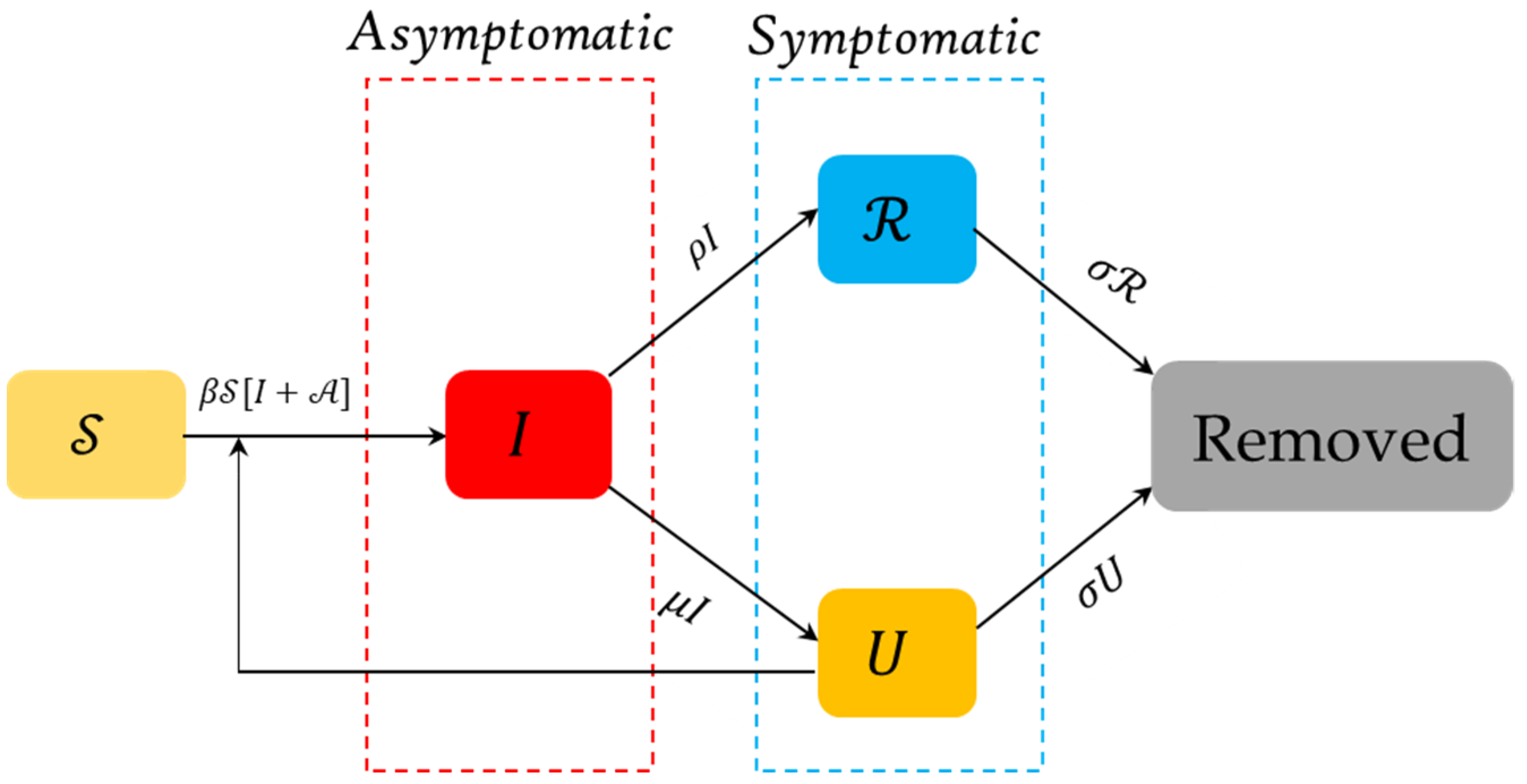
3. Mathematical Formulation of the SIRU Model

In [21], Liu et al. considered an epidemic model to depict the spread of 2019-nCoV. In particular, they investigated the evolution of the virus on data collected up to 31 January 2020 and presented some numerical simulations based on their model. In [21], the authors considered the interaction of four categories of individuals, viz., susceptible S$\left(t\right)$, asymptomatic infectious $I\left(t\right)$, symptomatic infectious $R\left(t\right)$ and unreported symptomatic infectious $U\left(t\right)$ at time $t$, thus obtaining the following system:

$$\begin{array}{c}\frac{dS\left(t\right)}{dt}=-\beta S\left(t\right)\left[I\left(t\right)+U\left(t\right)\right],\\ \frac{dI\left(t\right)}{dt}=\beta S\left(t\right)\left[I\left(t\right)+U\left(t\right)\right]-\gamma I\left(t\right),\\ \frac{dℛ\left(t\right)}{dt}=\rho I\left(t\right)-\sigma ℛ\left(t\right),\\ \frac{dU\left(t\right)}{dt}=\mu I\left(t\right)-\sigma U\left(t\right),\end{array}$$

(4)

where $\beta$ is the transmission rate, $\frac{1}{\gamma }$ and $\frac{1}{\sigma }$ represent, respectively, the average time elapsing for asymptomatic infectious and symptomatic infectious individuals before showing detectable symptoms, $\rho$ is the rate at which asymptomatic infectious individuals are reported as symptomatic and $\mu$ is the rate at which asymptomatic infectious individuals are unreported as symptomatic. The authors derived some essential conditions for the system to be symptomatic infectious and asymptomatic infectious. Further, they investigated the classical order system with the prediction forward in time for the severity of the epidemic. The interaction scheme is presented in Figure 1.

In this paper, we considered the fractional-order generalization of the above model (4) with the help of fractional calculus. The concept of fractional calculus (FC) was developed soon after classical calculus, but recently, many researchers have been magnetized towards the investigation of FC. In this connection, there are several fractional operators in both integration and differentiation, namely, Riemann–Liouville, Caputo, Grünwald–Letnikov, Riesz, Miller–Ross, Caputo–Fabrizio, Atangana–Baleanu and other fractional derivatives. Each operator has its own limitation and advantage. The Riemann–Liouville (RL) fractional operator has many limitations, including the classical physical properties of the function in which the derivative of the constant should be zero, whereas in the case of the RL operator, it will be non-zero. Further, we need to change the initial conditions to the fractional order when using an RL operator for initial value problems. These limitations are overcome by the Caputo fractional operator. The Riemann–Liouville derivative is based on power law, and it provides a description of real-world problems with lots of additional information that can be seen as noise or error due to specific memory properties. However, the new fractional operators are astounded by this drawback. The singular and kernel are the two pivotal properties of the differential system that exemplifies real-world phenomena. These properties are effectively incorporated in the newly defined operators with a fractional order by scholars [35,36]. Recently, it has been proved by many researchers that the Caputo fractional operator is more reliable in examining real-world problems, and this is the only operator with diverse generalized definitions based on the requirement of the particular phenomena [37,38,39,40,41]. In this connection, the authors in [42] examined a nonlinear system with the help of the Laplace transform and Caputo fractional derivative. Additionally, many researchers used fractional operators to examine and derive some stimulating consequences of physical phenomena [43,44]. Recently, scholars in [45] captured the complex natured quintic Ginzburg–Landau equation. The fifth-order weakly nonlocal fractional Schrödinger equation was studied with the Caputo derivative in [46].

We modified Equation (4) in order to incorporate memory and hereditary properties in the consideration. In particular, since the individuals with pre-existing diseases are prone to receive the 2019-nCoV infection, we considered the infection term by a fractional integral incorporating ($\beta \mathcal{S}\left(t\right)\left(J^{\alpha }I\left(t\right)+U\left(t\right)\right)$ so that Equation (4) is generalized as follows:

$$\begin{array}{c}{D}_t^{\alpha }\mathcal{S}\left(t\right)=-\beta \mathcal{S}\left(t\right)\left[J^{\alpha }I\left(t\right)+U\left(t\right)\right],\\ D_t^{\alpha }I\left(t\right)=\beta \mathcal{S}\left(t\right)\left(J^{\alpha }I\left(t\right)+U\left(t\right)\right)-\gamma I\left(t\right),\\ D_t^{\alpha }ℛ\left(t\right)=\rho I\left(t\right)-\sigma ℛ\left(t\right),\\ D_t^{\alpha }U\left(t\right)=\mu I\left(t\right)-\sigma U\left(t\right).\end{array}$$

(5)

Compared with system (4) in the modified system, the main differences are the following:

(1)

The system considered in Equation (4) depends on the ordinary derivative, which is the local operator, while Equation (5) depends on the fractional derivative, which, according to the definition of the Caputo derivative, takes into account some memory effect.

(2)

The dependence on an additional parameter, the fractional-order parameter, provides an additional degree of freedom, enabling it to fit better with the experimental data.

(3)

The fractional integrals on the right-hand side of system (5) describe the hereditariness of this phenomenon.

(4)

When α = 1, this system becomes the ordinary SIRU model, thus being a good candidate for a generalization.

4. Numerical Method for the Fractional-Order Equation

In this section, we describe the Adams–Bashforth–Moulton technique suitably adapted to solve the nonlinear fractional integro-differential equation of the form

$$D^{\alpha }y\left(t\right)=f\left(t,y\left(t\right)\right)+\lambda y\left(t\right)J^{\beta }y\left(t\right).$$

(6)

Let

$$g\left(t,y\left(t\right)\right)=f\left(t,y\left(t\right)\right)+\lambda y\left(t\right)J^{\beta }y\left(t\right).$$

(7)

Then, Equation (6) reduces to

$$D^{\alpha }y\left(t\right)=g\left(t,y\left(t\right)\right).$$

(8)

The Volterra integral equation corresponding to Equation (8) may be written as

$$y\left(t\right)={\displaystyle {\displaystyle \sum }_{m=0}^{\lceil \alpha \rceil -1}}\frac{y_0^{\left(m\right)}{t}^m}{m!}+\frac{1}{\mathsf{\Gamma }\left(\alpha \right)}\underset{0}{\overset{t}{{\displaystyle \int }}}{\left(t-\tau \right)}^{\alpha -1}g\left(\tau ,y\left(\tau \right)\right)d\tau .$$

(9)

In order to integrate (9), the Adams–Bashforth–Moulton method was used by setting $h=\frac{T}{N}, t_n=nh, n=0,1,2,\dots ,N\in {\mathbb{Z}}^{+}$. Now, Equation (9) can be written as

$$y\left(t_{n+1}\right)={\displaystyle {\displaystyle \sum }_{m=0}^{\lceil \alpha \rceil -1}}\frac{y_0^{\left(m\right)}{t}^m}{m!}+\frac{h^{\alpha }}{\mathsf{\Gamma }\left(\alpha +2\right)}g\left(t_{n+1},y^P\left(t_{n+1}\right)\right)+\frac{h^{\alpha }}{\mathsf{\Gamma }\left(\alpha +2\right)}{\displaystyle {\displaystyle \sum }_{j=0}^n}{a}_{j,n+1}g\left(t_j,y\left(t_j\right)\right),$$

(10)

where

$$y^P\left(t_{n+1}\right)={\displaystyle {\displaystyle \sum }_{m=0}^{\lceil \alpha -\rceil 1}}\frac{y_0^{\left(m\right)}{t}^m}{m!}+\frac{h^{\alpha }}{\mathsf{\Gamma }\left(\alpha +1\right)}{\displaystyle {\displaystyle \sum }_{j=0}^n}{b}_{j,n+1}g\left(t_j,y\left(t_j\right)\right).$$

(11)

The fractional integration $J^{\beta }y\left(t\right)$ is replaced by using a trapezoidal quadrature formula where the nodes $t_k \left(k=0,1,2,\dots ,n+1\right)$ are taken with respect to the weight function ${\left(t_k-.\right)}^{\beta -1}.$ We approximate $J^{\beta }y\left(t\right)$ as

$$J^{\beta }y\left(t\right)=\frac{h^{\beta }}{\mathsf{\Gamma }\left(\beta +2\right)}{\displaystyle {\displaystyle \sum }_{k=0}^{n+1}}{d}_{k,n+1}y\left(t_k\right).$$

(12)

Therefore, the predictor–corrector formula for Equation (6) may be written as follows:

$$y^P\left(t_{n+1}\right)={\displaystyle {\displaystyle \sum }_{m=0}^{\lceil \alpha \rceil -1}}\frac{y_0^{\left(m\right)}{t}^m}{m!}+\frac{h^{\alpha }}{\mathsf{\Gamma }\left(\alpha +1\right)}{\displaystyle {\displaystyle \sum }_{j=0}^n}{b}_{j,n+1}(f(t_j,y\left(t_j\right)+\lambda y\left(t_j\right)\frac{h^{\beta }}{\mathsf{\Gamma }\left(\beta +2\right)}{\displaystyle {\displaystyle \sum }_{k=0}^j}{d}_{k,j}y\left(t_k\right)),$$

(13)

and

$$\begin{array}{c}y\left(t_{n+1}\right)={\displaystyle {\displaystyle \sum }_{m=0}^{\lceil \alpha \rceil -1}}\frac{y_0^{\left(m\right)}{t}^m}{m!}\hfill \\ +\frac{h^{\alpha }}{\mathsf{\Gamma }\left(\alpha +2\right)}(f\left(t_{n+1},y^P\left(t_{n+1}\right)\right)\hfill \\ +\lambda y\left(t_j\right)\frac{h^{\beta }}{\mathsf{\Gamma }\left(\beta +2\right)}{\displaystyle {\displaystyle \sum }_{k=0}^{n+1}}{d}_{k,n+1}{y}^P\left(t_k\right))\hfill \\ +\frac{h^{\alpha }}{\mathsf{\Gamma }\left(\alpha +2\right)}{\displaystyle {\displaystyle \sum }_{j=0}^n}{a}_{j,n+1}(f(t_j,y\left(t_j\right)+\lambda y\left(t_j\right)\frac{h^{\beta }}{\mathsf{\Gamma }\left(\beta +2\right)}{\displaystyle {\displaystyle \sum }_{k=0}^j}{d}_{k,j}y\left(t_k\right),\hfill \end{array}$$

(14)

$$a_{i,n+1}=\left(\begin{array}{ll}{n}^{\alpha +1}-\left(n-\alpha \right){(n+1)}^{\alpha },\hfill & i=0,\hfill \\ {(n-i+2)}^{\alpha +1}+{(n-i)}^{\alpha +1}-2{(n-i+1)}^{\alpha +1},\hfill & 1\le i\le n,\hfill \\ 1,\hfill & i=n+1,\hfill \end{array}\right)$$

(15)

$$d_{k,n+1}=\left(\begin{array}{ll}{n}^{\beta +1}-\left(n-\beta \right){(n+1)}^{\beta },\hfill & k=0,\hfill \\ {(n-k+2)}^{\beta +1}+{(n-k)}^{\beta +1}-2{(n-k+1)}^{\beta +1},\hfill & 1\le k\le n,\hfill \\ 1,\hfill & k=n+1,\hfill \end{array}\right)$$

(16)

and

$$b_{i,n+1}={\left(n-i+1\right)}^{\alpha }-{\left(n-i\right)}^{\alpha },0\le i\le n.$$

(17)

5. Solution for the Projected Models

By taking into account the generalized Adam–Bashfort–Moulton method as given in the previous section, Equation (5) can be written as follows:

$$\begin{array}{cc}\hfill S_{n+1}& =S_0+\frac{h^{\alpha }}{\mathsf{\Gamma }\left(\alpha +2\right)}\left(-\beta S_{n+1}^P\left(\frac{h^{\alpha }}{\mathsf{\Gamma }\left(\alpha +2\right)}{\displaystyle {\displaystyle \sum }_{k=0}^{n+1}}{d}_{k,n+1}{I}_k^P+U_{n+1}^P\right)\right)\hfill \\ & +\frac{h^{\alpha }}{\mathsf{\Gamma }\left(\alpha +2\right)}{\displaystyle {\displaystyle \sum }_{j=0}^n}{a}_{j,n+1}\left(-\beta S_j\left(\frac{h^{\alpha }}{\mathsf{\Gamma }\left(\alpha +2\right)}{\displaystyle {\displaystyle \sum }_{k=0}^{n+1}}{d}_{k,n+1}{I}_j+U_j\right)\right),\hfill \\ \hfill I_{n+1}& =I_0+\frac{h^{\alpha }}{\mathsf{\Gamma }\left(\alpha +2\right)}\left(\beta S_{n+1}^P\left(\frac{h^{\alpha }}{\mathsf{\Gamma }\left(\alpha +2\right)}{\displaystyle {\displaystyle \sum }_{k=0}^{n+1}}{d}_{k,n+1}{I}_k^P+U_{n+1}^P\right)-\gamma I_{n+1}^P\right)\hfill \\ & +\frac{h^{\alpha }}{\mathsf{\Gamma }\left(\alpha +2\right)}{\displaystyle {\displaystyle \sum }_{j=0}^n}{a}_{j,n+1}\left(-\beta S_j\left(\frac{h^{\alpha }}{\mathsf{\Gamma }\left(\alpha +2\right)}{\displaystyle {\displaystyle \sum }_{k=0}^{n+1}}{d}_{k,n+1}{I}_j+U_j\right)-\gamma I_j\right),\hfill \\ \hfill R_{n+1}& =R_0+\frac{h^{\alpha }}{\mathsf{\Gamma }\left(\alpha +2\right)}\left(\rho I_{n+1}^P-\sigma R_{n+1}^P\right)+\frac{h^{\alpha }}{\mathsf{\Gamma }\left(\alpha +2\right)}{\displaystyle {\displaystyle \sum }_{j=0}^n}{a}_{j,n+1}\left(\rho I_j-\sigma R_j\right),\hfill \\ \hfill U_{n+1}& =U_0+\frac{h^{\alpha }}{\mathsf{\Gamma }\left(\alpha +2\right)}\left(\mu I_{n+1}^P-\sigma U_{n+1}^P\right)+\frac{h^{\alpha }}{\mathsf{\Gamma }\left(\alpha +2\right)}{\displaystyle {\displaystyle \sum }_{j=0}^n}{a}_{j,n+1}\left(\rho I_j-\sigma U_j\right),\hfill \end{array}$$

(18)

where

$$\begin{array}{c}{S}_{n+1}^P=S_0+\frac{h^{\alpha }}{\mathsf{\Gamma }\left(\alpha +1\right)}{\displaystyle {\displaystyle \sum }_{j=0}^n}{b}_{j,n+1}\left(-\beta S_j\left(\frac{h^{\alpha }}{\mathsf{\Gamma }\left(\alpha +2\right)}{\displaystyle {\displaystyle \sum }_{k=0}^{n+1}}{d}_{k,n+1}{I}_j+U_j\right)\right),\\ I_{n+1}^P=I_0+\frac{h^{\alpha }}{\mathsf{\Gamma }\left(\alpha +1\right)}{\displaystyle {\displaystyle \sum }_{j=0}^n}{b}_{j,n+1}\left(-\beta S_j\left(\frac{h^{\alpha }}{\mathsf{\Gamma }\left(\alpha +2\right)}{\displaystyle {\displaystyle \sum }_{k=0}^{n+1}}{d}_{k,n+1}{I}_j+U_j\right)-\gamma I_j\right),\\ R_{n+1}^P=R_0+\frac{h^{\alpha }}{\mathsf{\Gamma }\left(\alpha +1\right)}{\displaystyle {\displaystyle \sum }_{j=0}^n}{a}_{j,n+1}\left(\rho I_j-\sigma R_j\right),\\ U_{n+1}^P=U_0+\frac{h^{\alpha }}{\mathsf{\Gamma }\left(\alpha +1\right)}{\displaystyle {\displaystyle \sum }_{j=0}^n}{a}_{j,n+1}\left(\rho I_j-\sigma U_j\right).\end{array}$$

(19)

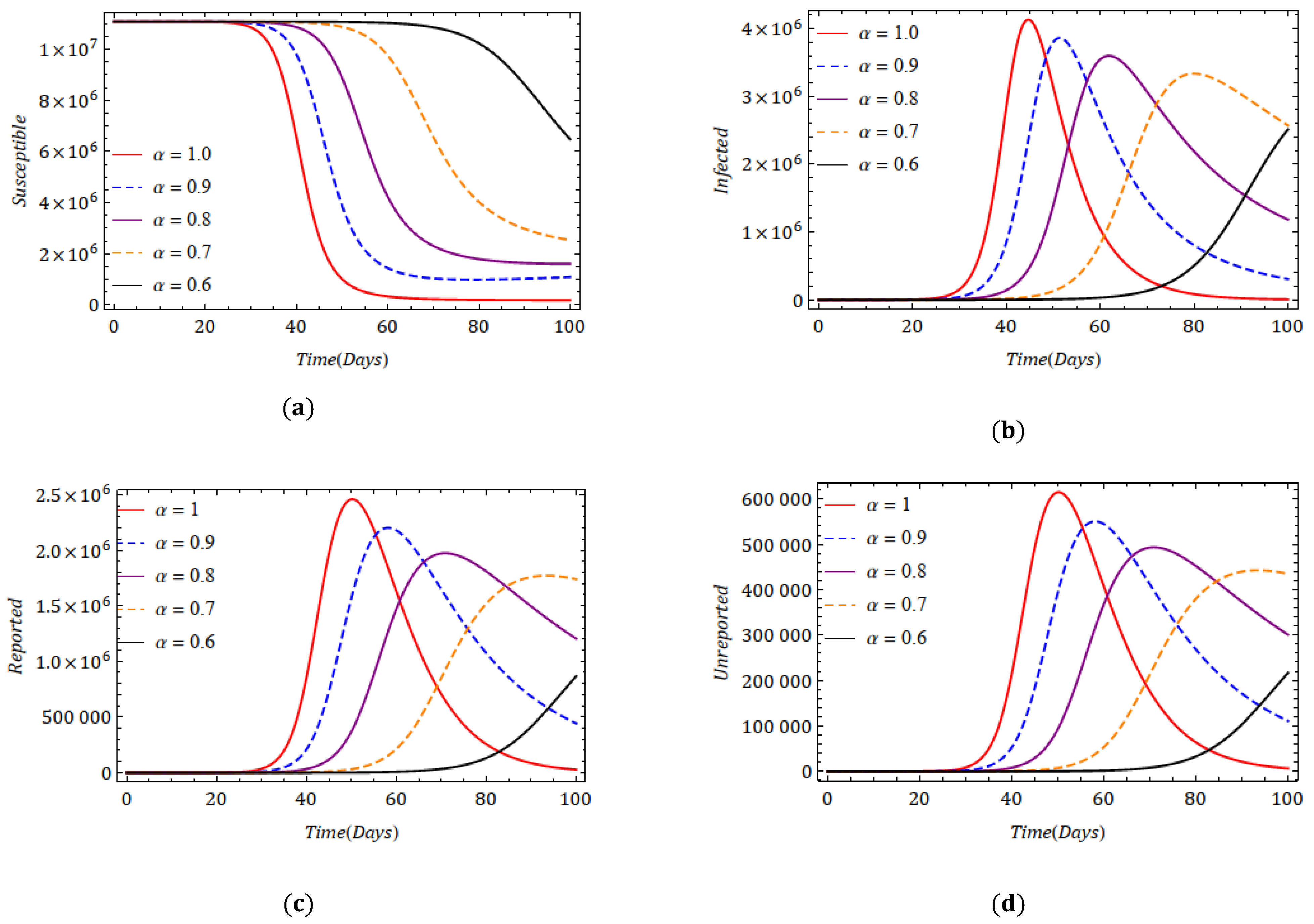
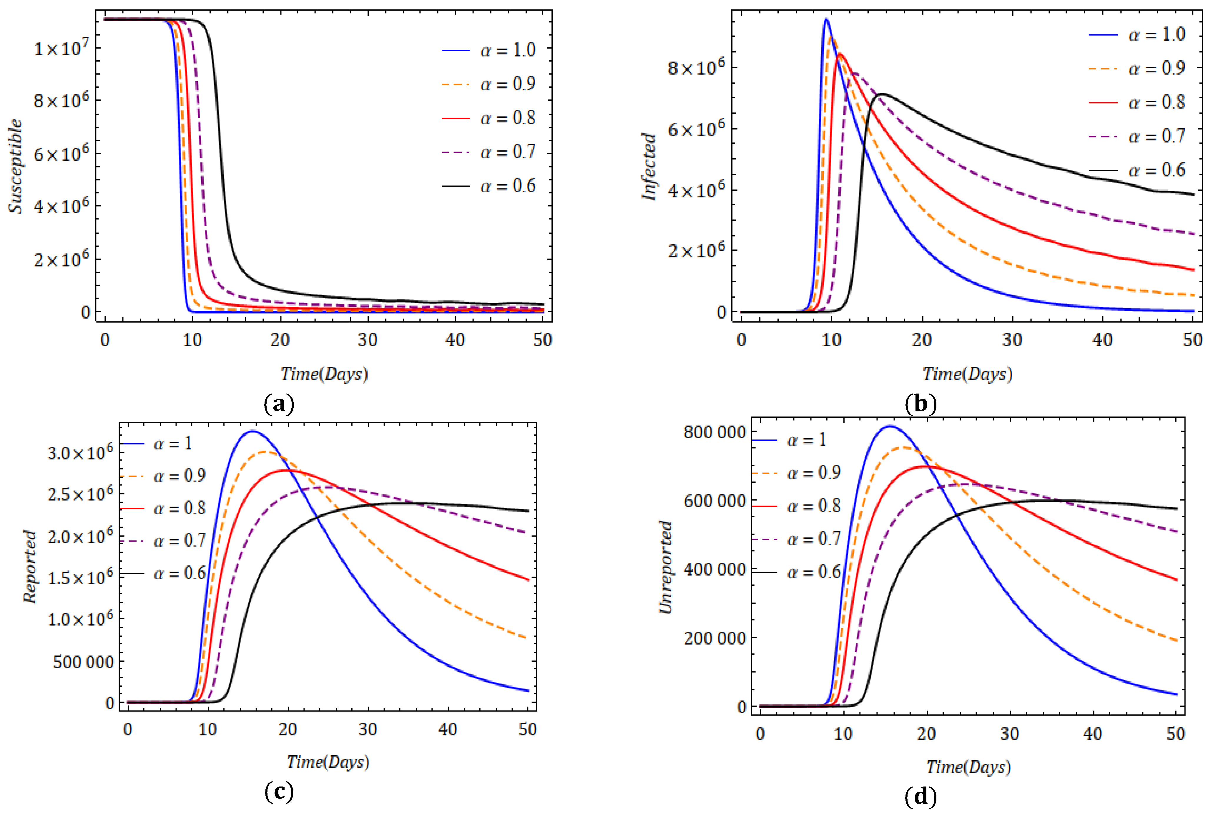
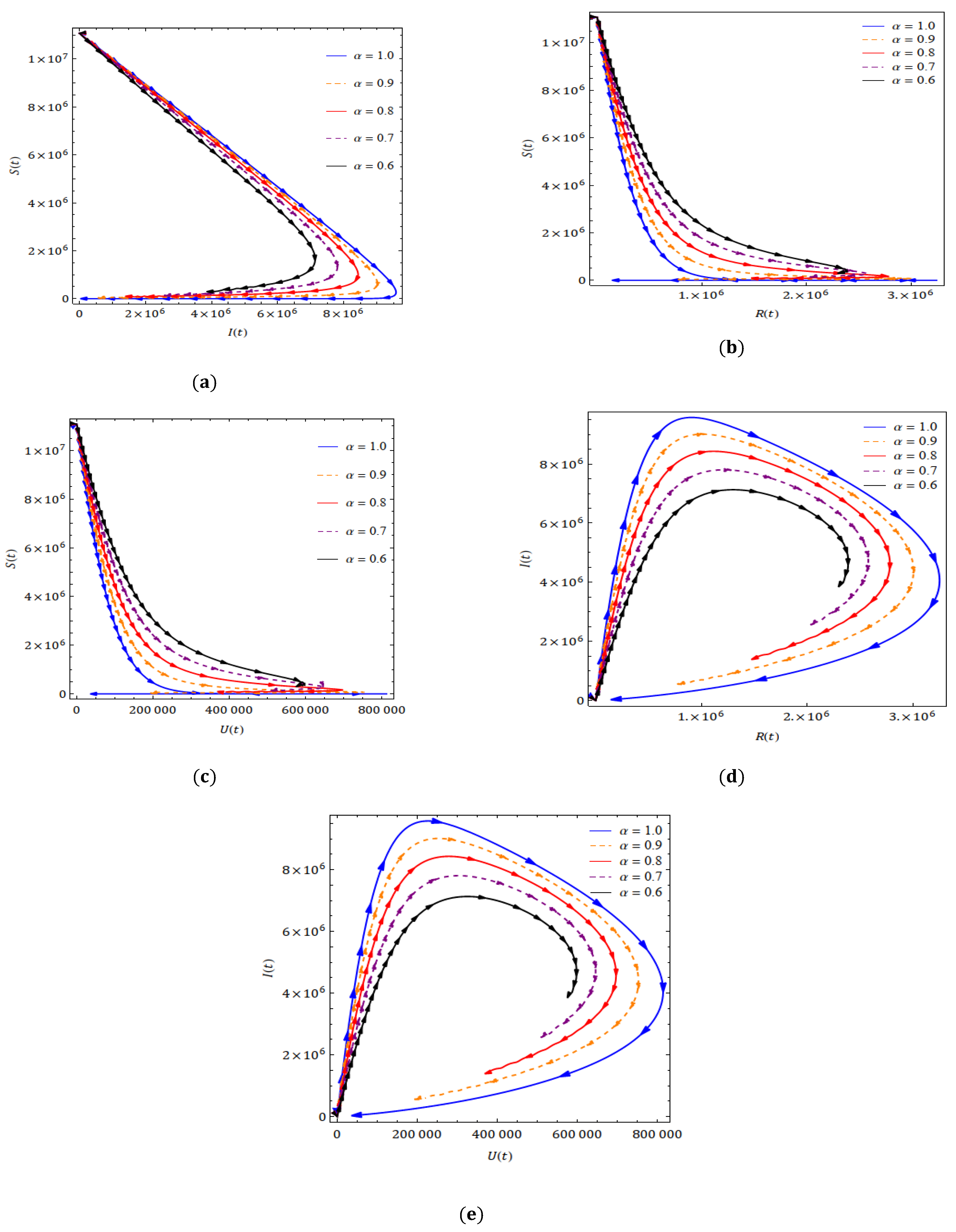
6. Results and Conclusions

In order to show the efficiency of this method, we present a numerical simulation by assuming the initial conditions as $S\left(0\right)=S_0=11.081\times {10}^6, I\left(0\right)=I_0=3.62, R\left(0\right)=R_0=0$ and $U\left(0\right)=U_0=0.2$. In order to compare this numerical simulation with the results obtained in [21] for the remaining parameters, we assume

$$\beta =4.44\times {10}^{-8}, \gamma =\frac{1}{7}, \sigma =\frac{1}{7}, \rho =0.8 \gamma \mathrm{and} \mu =0.2 \gamma .$$

To compare the results of the modified model (5) with model (4) projected in [21], in Figure 2 and Figure 3, we present the graphical representation of the nature of the various categories of the population in the presence of the fractional derivative. A comparison is presented in Figure 2 for model (4), and we observe that the evidence of the infection starts rising approximately after 30 days. As a result, a similar effect can be observed in other populations, viz., a fall in the non-infected population, a rise in the reported population and a rise in the unreported population. However, in Figure 3 for model (5), we observe that a rapid increase in the infection and exponential spreading occurs in less than 10 days. We assume that 80% of cases are reported and 20% of cases are not reported. For $\alpha =1$, even though the peak of infection was attained very fast, the decline was also attained quickly (Figure 3b). Reported and unreported populations show a similar pattern (Figure 3c,d). As the values of the fractional derivative decline from 1 to 0.6 gradually, we observe that the maximum number of infected individuals is less, but infection stays in the population for a longer duration. We can claim that the fractional-order derivative helps us model the spread of the COVID-19 epidemic among people with pre-existing infections such as cancer, chronic kidney disease, chronic lung diseases, diabetes and HIV infection. Moreover, the coronavirus infection will never be eradicated from the population. In some corners of some countries, some individuals will always remain infected. The fractional dynamics can only depict this non-elimination nature.

In Figure 4, we cite the representation of the solution trajectories of $I\left(t\right) vs. S\left(t\right)$,$R\left(t\right) vs. S\left(t\right)$, $U\left(t\right) vs. S\left(t\right), R\left(t\right) vs. I\left(t\right)$ and $U\left(t\right) vs. I\left(t\right)$ for various values of $\alpha$ for a time period of 50 days. In Figure 4a, we observe that the infected population is inversely proportional to the susceptible population with increasing time to a certain point. After that point, even though the infection reduces, the susceptible population also shows a declining trend. This is mainly due to the time taken for recovery. We observe that in 50 days, solution curves approach $\left(1.128\times {10}^4,5.159\times {10}^4\right)$ for $\alpha =1,\left(6.026\times {10}^5,5.159\times {10}^4\right)$ for $\alpha =0.9$, $\left(1.4\times {10}^6,8.128\times {10}^4\right)$ for $\alpha =0.8$, $\left(2.582\times {10}^6,1.704\times {10}^5\right)$ for $\alpha =0.7$ and $\left(3.868\times {10}^6,3.189\times {10}^5\right)$ for $\alpha =0.6$. During the outbreak of the 2019-nCoV pandemic, in reality, we have seen that infection remained at a comparatively higher level in 50 days. This indicates that the fractional derivative provides a more reliable prediction. In Figure 4b–e, we can observe a similar type of interpretation.

Parameters such as rate of infection, the average time during which asymptomatic infectious individuals are asymptomatic, the rate at which asymptomatic infectious individuals report becoming symptomatic and the rate at which asymptomatic infectious individuals are unreported as symptomatic have a significant influence in controlling the spread of the pandemic. Hence, it is essential and important to investigate its outbreak and behavior with different parameters to analyze and predict its evolution and spread. In Figure 5 and Figure 6, we present the impact of the transmission rate on various populations for $\alpha =1$ and $\alpha =0.9,$ respectively. We observe that an increase in the rate of disease transmission speeds up the increase in infection. However, the attained peak for $\alpha =1$ is higher than that for $\alpha =0.9$. The result obtained for $\alpha =0.9$ looks more believable because the declining trend of the infection is slower here. Figure 7 depicts the impact of the fractional derivative and average time during which asymptomatic infectious individuals are asymptomatic on infected, reported and unreported populations. In Figure 8, we present the influence of the rate of reported and unreported populations in the frame of the fractional derivative. The proportionate changes in reported and unreported rates do not affect the infected population.

The present investigation may help researchers understand some stimulating consequences of the considered model. From the plots, for the change in $\alpha$, the obtained solution presents fascinating consequences with a fixed value of the parameters defined in the considered system. Finally, we can see that the projected solution technique is highly efficient in solving a nonlinear system of fractional differential equations describing the novel virus.

References

1. Estola, T. Coronaviruses, a New Group of Animal RNA Viruses. Avian Dis. 1970, 14, 330. [Google Scholar] [CrossRef] [PubMed]
2. Kahn, J.S.; McIntosh, K. History and Recent Advances in Coronavirus Discovery. Pediatr. Infect. Dis. J. 2005, 24, S223–S227. [Google Scholar] [CrossRef]
3. Worldometer, COVID-19 Coronavirus Pandemic. Available online: https://www.worldometers.info/coronavirus/ (accessed on 5 July 2020).
4. Riemann, G.F.B. Versucheinerallgemeinen Auffassung der Integration und Differentiation. Gesammelte Math. Werke Leipz. 1896, 62, 331–344. [Google Scholar]
5. Caputo, M. Elasticita e Dissipazione; Zanichelli: Bologna, Italy, 1969. [Google Scholar]
6. Miller, K.S.; Ross, B. An Introduction to Fractional Calculus and Fractional Differential Equations; Wiley: New York, NY, USA, 1993. [Google Scholar]
7. Podlubny, I. Fractional Differential Equations; Academic Press: New York, NY, USA, 1999. [Google Scholar]
8. Kilbas, A.A.; Srivastava, H.M.; Trujillo, J.J. Theory and Applications of Fractional Differential Equations; North-Holland Mathematical Studies; Elsevier (North-Holland) Science Publishers: Amsterdam, The Netherlands, 2006; Volume 204. [Google Scholar]
9. Baleanu, D.; Guvenc, Z.B.; Tenreiro Machado, J.A. New Trends in Nanotechnology and Fractional Calculus Applications; Springer: Berlin/Heidelberg, Germany, 2010. [Google Scholar]
10. Baleanu, D.; Wu, G.-C.; Zeng, S. Chaos analysis and asymptotic stability of generalized Caputo fractional differential equations. Chaos Solitons Fractals 2017, 102, 99–105. [Google Scholar] [CrossRef]
11. Veeresha, P.; Prakasha, D.G.; Baskonus, H.M. New numerical surfaces to the mathematical model of cancer chemotherapy effect in Caputo fractional derivatives. Chaos Interdiscip. J. Nonlinear Sci. 2019, 29, 013119. [Google Scholar] [CrossRef]
12. Alkahtani, B.S.T.; Atangana, A. Analysis of non-homogeneous heat model with new trend of derivative with fractional order. Chaos Solitons Fractals 2016, 89, 566–571. [Google Scholar] [CrossRef]
13. Veeresha, P.; Ilhan, E.; Baskonus, H.M. Fractional approach for analysis of the model describing wind-influenced projectile motion. Phys. Scr. 2021, 96, 075209. [Google Scholar] [CrossRef]
14. Veeresha, P.; Prakasha, D. Solution for fractional generalized Zakharov equations with Mittag-Leffler function. Results Eng. 2020, 5, 100085. [Google Scholar] [CrossRef]
15. Khan, M.A.; Atangana, A. Modeling the dynamics of novel coronavirus (2019-nCov) with fractional derivative. Alex. Eng. J. 2020, 59, 2379–2389. [Google Scholar] [CrossRef]
16. Chen, T.-M.; Rui, J.; Wang, Q.-P.; Zhao, Z.-Y.; Cui, J.-A.; Yin, L. A mathematical model for simulating the phase-based transmissibility of a novel coronavirus. Infect. Dis. Poverty 2020, 9, 24. [Google Scholar] [CrossRef] [Green Version]
17. Li, Y.; Wang, B.; Peng, R.; Zhou, C.; Zhan, Y.; Zhang, X.; Jiang, X.; Zhao, B. Mathematical Modeling and Epidemic Prediction of Covid-19 and Its Significance to Epidemic Prevention and Control Measures. J. Surg. Case Rep. Images 2020, 1, 1–19. [Google Scholar] [CrossRef]
18. Gao, W.; Veeresha, P.; Prakasha, D.G.; Baskonus, H.M. Novel Dynamic Structures of 2019-nCoV with Nonlocal Operator via Powerful Computational Technique. Biology 2020, 9, 107. [Google Scholar] [CrossRef] [PubMed]
19. Atangana, A. Modelling the spread of COVID-19 with new fractal-fractional operators: Can the lockdown save mankind before vaccination? Chaos Solitons Fractals 2020, 136, 109860. [Google Scholar] [CrossRef]
20. Gao, W.; Veeresha, P.; Baskonus, H.M.; Prakasha, D.G.; Kumar, P. A new study of unreported cases of 2019-nCOV epidemic outbreaks. Chaos Solitons Fractals 2020, 138, 109929. [Google Scholar] [CrossRef] [PubMed]
21. Liu, Z.; Magal, P.; Seydi, O.; Webb, G. Understanding Unreported Cases in the COVID-19 Epidemic Outbreak in Wuhan, China, and the Importance of Major Public Health Interventions. Biology 2020, 9, 50. [Google Scholar] [CrossRef] [PubMed] [Green Version]
22. Din, R.U.; Shah, K.; Ahmad, I.; Abdeljawad, T. Study of transmission dynamics of novel COVID-19 by using mathematical model. Adv. Differ. Equations 2020, 2020, 323. [Google Scholar] [CrossRef]
23. Kiran, M.S.; Betageri, V.; Prakasha, D.G.; Veeresha, P.; Kumar, S. A mathematical analysis of ongoing outbreak COVID-19 in India through nonsingular derivative. Numer. Methods Partial Differ. Equ. 2021, 37, 1282–1298. [Google Scholar] [CrossRef]
24. Rahman, G.U.; Shah, K.; Haq, F.; Ahmad, N. Host vector dynamics of pine wilt disease model with convex incidence rate. Chaos Solitons Fractals 2018, 113, 31–39. [Google Scholar] [CrossRef]
25. Lu, R.; Zhao, X.; Li, J.; Niu, P.; Yang, B.; Wu, H.; Wang, W.; Song, H.; Huang, B.; Zhu, N.; et al. Genomic characterisation and epidemiology of 2019 novel coronavirus: Implications for virus origins and receptor binding. Lancet 2020, 395, 565–574. [Google Scholar] [CrossRef] [Green Version]
26. Buonomo, B.; Lacitignola, D. On the dynamics of an SEIR epidemic model with a convex incidence rate. Ric. Mat. 2008, 57, 261–281. [Google Scholar] [CrossRef]
27. Lin, Q.; Zhao, S.; Gao, D.; Lou, Y.; Yang, S.; Musa, S.S.; Wang, M.H.; Cai, Y.; Wang, W.; Yang, L.; et al. A conceptual model for the coronavirus disease 2019 (COVID-19) outbreak in Wuhan, China with individual reaction and governmental action. Int. J. Infect. Dis. 2020, 93, 211–216. [Google Scholar] [CrossRef] [PubMed]
28. Ndaïrou, F.; Area, I.; Nieto, J.J.; Torres, D.F. Mathematical modeling of COVID-19 transmission dynamics with a case study of Wuhan. Chaos Solitons Fractals 2020, 135, 109846. [Google Scholar] [CrossRef] [PubMed]
29. Baishya, C.; Veeresha, P. Laguerre polynomial-based operational matrix of integration for solving fractional differential equations with non-singular kernel. Proc. R. Soc. A 2021, 477, 20210438. [Google Scholar] [CrossRef]
30. Diethelm, K.; Ford, N. Analysis of Fractional Differential Equations. J. Math. Anal. Appl. 2002, 265, 229–248. [Google Scholar] [CrossRef] [Green Version]
31. Baishya, C. An operational matrix based on the Independence polynomial of a complete bipartite graph for the Caputo fractional derivative. SeMA J. 2021, 68, 2. [Google Scholar] [CrossRef]
32. Baishya, C.; Achar, S.J.; Veeresha, P.; Prakasha, D.G. Dynamics of a fractional epidemiological model with disease infection in both the populations. Chaos: Interdiscip. J. Nonlinear Sci. 2021, 31, 043130. [Google Scholar] [CrossRef]
33. Baishya, C. Dynamics of fractional stage structured predator prey model with prey refuge. Indian J. Ecol. 2020, 47, 1118–1124. [Google Scholar]
34. Achar, S.J.; Baishya, C.; Kaabar, M.K.A. Dynamics of the worm transmission in wireless sensor network in the framework of fractional derivatives. Math. Methods Appl. Sci. 2021, 1–17. [Google Scholar] [CrossRef]
35. Caputo, M.; Fabrizio, M. A new definition of fractional derivative without singular kernel. Progr. Fract. Differ. Appl. 2015, 1, 1–13. [Google Scholar]
36. Atangana, A.; Baleanu, D. New fractional derivatives with nonlocal and non-singular kernel: Theory and application to heat transfer mode. Therm. Sci. 2016, 20, 763–769. [Google Scholar] [CrossRef] [Green Version]
37. Abdel-Gawad, H.I.; Tantawy, M. Traveling Wave Solutions of DNA-Torsional Model of Fractional Order. Appl. Math. Inf. Sci. Lett. 2018, 6, 85–89. [Google Scholar] [CrossRef]
38. Kausar, H.; Adhami, A.Y. A Fuzzy Goal Programming Approach for Solving Chance Constrained Bi-Level Multi-Objective Quadratic Fractional Programming Problem. Appl. Math. Inf. Sci. Lett. 2019, 7, 27–35. [Google Scholar] [CrossRef]
39. Gao, W.; Veeresha, P.; Prakasha, D.G.; Senel, B.; Baskonus, H.M. Iterative method applied to the fractional nonlinear systems arising in thermoelasticity with Mittag-Leffler kernel. Fractals 2020, 28, 2040040. [Google Scholar] [CrossRef]
40. Aghili, A. Complete Solution For The Time Fractional Diffusion Problem With Mixed Boundary Conditions by Operational Method. Appl. Math. Nonlinear Sci. 2021, 6, 9–20. [Google Scholar] [CrossRef] [Green Version]
41. Mustafa, G.; Yıldız, Ç. Some new inequalities for convex functions via Riemann-Liouville fractional integrals. Appl. Math. Nonlinear Sci. 2021, 6, 537–544. [Google Scholar]
42. Malagi, N.S.; Veeresha, P.; Prasannakumara, B.; Prasanna, G.; Prakasha, D. A new computational technique for the analytic treatment of time-fractional Emden–Fowler equations. Math. Comput. Simul. 2021, 190, 362–376. [Google Scholar] [CrossRef]
43. Akdemir, A.O.; Deniz, E.; Yüksel, E. On Some Integral Inequalities via Conformable Fractional Integrals. Appl. Math. Nonlinear Sci. 2020, 6, 489–498. [Google Scholar] [CrossRef]
44. Touchent, K.A.; Hammouch, Z.; Mekkaoui, T. A modified invariant subspace method for solving partial differential equations with non-singular kernel fractional derivatives. Appl. Math. Nonlinear Sci. 2020, 5, 35–48. [Google Scholar] [CrossRef]
45. Yao, S.-W.; Ilhan, E.; Veeresha, P.; Baskonus, H.M. A Powerful Iterative Approach for Quintic Complex Ginzburg–Landau Equation within the Frame of Fractional Operator. Fractals 2021, 29, 2140023. [Google Scholar] [CrossRef]
46. Akinyemi, L.; Nisar, K.S.; Saleel, C.A.; Rezazadeh, H.; Veeresha, P.; Khater, M.M.; Inc, M. Novel approach to the analysis of fifth-order weakly nonlocal fractional Schrödinger equation with Caputo derivative. Results Phys. 2021, 31, 104958. [Google Scholar] [CrossRef]
Figure 1. Schematic diagram of the model defined in Equation (4) [21].
Fractalfract 06 00092 g001
Figure 2. Behavior of obtained results for (a) S ( t ) , (b) I ( t ) , (c) ( t ) and (d) U ( t ) for a distinct fractional order ( α ) for system (4) with a fractional derivative.
Fractalfract 06 00092 g002
Figure 3. Behavior of obtained results for (a) S ( t ) , (b) I ( t ) , (c) ( t ) and (d) U ( t ) at a distinct fractional order ( α ) for system (5).
Fractalfract 06 00092 g003
Figure 4. Parametric nature of obtained results at a distinct fractional order ( α ) with (a) I ( t )   v s .   S ( t ) , (b) R ( t )   v s .   S ( t ) , (c) U ( t )   v s .   S ( t ) , (d) R ( t )   v s .   I ( t ) and (e) U ( t )   v s .   I ( t ) for system (5).
Fractalfract 06 00092 g004
Figure 5. Effect of rate of transmission on (a) S ( t ) , (b) I ( t ) , (c) ( t ) and (d) U ( t ) at a distinct fractional order α = 1   for   system   ( 5 ) .
Fractalfract 06 00092 g005
Figure 6. Effect of rate of transmission on (a) S ( t ) , (b) I ( t ) , (c) ( t ) and (d) U ( t ) at a distinct fractional order α = 0.9   for   system   ( 5 ) .
Fractalfract 06 00092 g006
Figure 7. Effect of average time during which asymptomatic infectious individuals are asymptomatic ( 1 γ ) (a) I ( t ) for   α = 1 , (b) ( t ) for α = 1 , (c) U ( t ) for α = 1 , (d) I ( t ) for α = 0.9 , (e) ( t ) for α = 0.9 , (f) U ( t ) for   α = 0.9 for system (5).
Fractalfract 06 00092 g007
Figure 8. Effect of rate of reported and unreported populations (a) I ( t ) for   α = 1 , (b) ( t ) for α = 1 , (c) U ( t ) for α = 1 , (d) I ( t ) for α = 0.9 , (e) ( t ) for α = 0.9 , (f) U ( t ) for   α = 0.9 for system (5).
Fractalfract 06 00092 g008
Publisher’s Note: MDPI stays neutral with regard to jurisdictional claims in published maps and institutional affiliations.