A New Iterative Predictor-Corrector Algorithm for Solving a System of Nuclear Magnetic Resonance Flow Equations of Fractional Order

Abstract

Nuclear magnetic resonance flow equations, also known as the Bloch system, are said to be at the heart of both magnetic resonance imaging (MRI) and nuclear magnetic resonance (NMR) spectroscopy. The main aim of this research was to solve fractional nuclear magnetic resonance flow equations (FNMRFEs) through a numerical approach that is very easy to handle. We present a New Iterative Predictor-Corrector Algorithm (NIPCA) based on the New Iterative Algorithm and Predictor-Corrector Algorithm to solve nonlinear nuclear magnetic resonance flow equations of fractional order involving Caputo derivatives. Graphical representation of the solutions with detailed error analysis shows the higher accuracy of the new technique. This New Iterative Predictor-Corrector Algorithm requires less computational time than previously published numerical methods. The results achieved in this article indicate that the algorithm is fit to use for other chaotic systems of fractional differential equations.

1. Introduction

Nuclear magnetic resonance provides the physical basis for a vast selection of methods that are usually used to investigate the dynamics of the structure of cells, tissues, etc., up to the extent of the entire body [1]. For example, chemists have recently studied biomolecules and their structural analysis using magnetic resonance spectroscopy (MRS), and MRI is a vital instrument in the radiology departments of hospitals. MRI helps construct a model of the soft tissue structures of the human spine and brain [2] with a resolution of sub-millimeter. By comparison, MRS helps in identifying individual bimolecular structural configurations with a resolution up to sub-nanometer. This provides a tremendously broad range of scales, providing the physician with a safe means to identify diseases and their stages, such as cancer, and provides chemists with a highly efficient instrument for understanding molecular synthesis. For more details, see [3,4,5,6,7].

Similarly, for discovering the molecular basis that underlies abnormal cell growth, spectroscopic and imaging information provides the necessary technological tools, in addition to helping in monitoring a unique tumor’s response to drugs or radiological treatments.

The typical means of defining NMR (i.e., “the phenomena that make up the inner workings of MRI”) in vector form is presented with the help of the Bloch equation. This equation corresponding to a uniform sample may be expressed as [8,9]:

$$\frac{d\overrightarrow{M}}{dt}=\gamma \left(\overrightarrow{M}\times \overrightarrow{B}\right)-\frac{M_z-M_o}{T_1^{\prime }}{\widehat{i}}_z-\frac{M_x{\widehat{i}}_x+M_y{\widehat{i}}_y}{T_2^{\prime }}$$

(1)

where $\overrightarrow{M}\left(M_x,M_y,M_z\right)$ is the time-varying system magnetization; $M_0$ represents the equilibrium magnetization; $\overrightarrow{B}\left(B_x,B_y,B_z\right)$ is the applied radio frequency $B_x$, gradient $B_y$, and static magnetic fields $B_z$; $\gamma$ is the gyro-magnetic ratio; and $T_1^{\prime }$ shows the spin-lattice relaxation time, giving the characterization of the rate at which the longitudinal $M_z$ component of the magnetization vector recovers. It has the property that it changes exponentially towards its thermodynamic equilibrium. $T_2^{\prime }$ is the spin-spin relaxation time, which gives the characterization of the signal decay in MRI and NMR, i.e., $T_2^{\prime }$ is the rate that corresponds to the exponential decay of the zero towards the transverse component of the magnetization vector, $M_{xy}=M_x{\widehat{i}}_x+M_y{\widehat{i}}_y$.

In this paper, we present, for the first time, a new technique for the numerical solution of fractional nuclear magnetic resonance flow equations, in the form of the technique of the New Iterative Predictor-Corrector Algorithm. In Section 2, we discuss nuclear magnetic resonance flow equations of fractional order, including information about the Caputo derivative. Section 3 describes a New Iterative Predictor-Corrector Algorithm specially formulated on nonlinear fractional nuclear magnetic resonance flow. In Section 4, the numerical simulation is presented. In the last section, a conclusive summary of the research is presented.

2. Application on Fractional Nuclear Magnetic Resonance Flow Equations

Nuclear magnetic resonance flow equations can be considered as a system of macroscopic equations. These equations estimate nuclear magnetization as a function of time $\overrightarrow{M}\left(M_x,M_y,M_z\right)$ with the relaxation times of spin-lattice $T_1^{\prime }$ and spin-spin $T_2^{\prime }$. Felix Bloch is the pioneer who first introduced these equations in 1946. Later developments in the research of fractional calculus have shown that a system of fractional order differential equations involving Caputo derivatives enables a mathematical description in the following form [10]:

$$\begin{array}{c}{D}_t^{\alpha }{M}_x\left(t\right)={\varpi }_{0 }^{\prime }{M}_y\left(t\right)-\frac{M_x\left(t\right)}{T_2^{\prime }}\hfill \\ D_t^{\beta }{M}_y\left(t\right)=-{\varpi }_0^{\prime }{M}_x\left(t\right)-\frac{M_y\left(t\right)}{T_2^{\prime }}\hfill \\ D_t^{\eta }{M}_z\left(t\right)=\frac{M_0-M_z\left(t\right)}{T_1^{\prime }}\hfill \end{array}$$

(2)

where $M_0$ is the equilibrium magnetization. The Larmor relationship provides the resonant frequency ${\varpi }_{0 }^{\prime }$ as: ${\varpi }_{0 }^{\prime }=\gamma B_0$. Here, $B_0$ is the constant static magnetic field. In the case of the gyro-magnetic ratio $\frac{\gamma }{2\pi }=\frac{f_0}{B_0}=42.57 \mathrm{MHz}/\mathrm{T}$ corresponding to water protons, we have ${\varpi }_{0 }^{\prime }=2\pi f_0$.

Moreover, in order to maintain consistency in setting the units measuring the magnetization, $s^{\overline{\alpha }}$ is chosen to express the measurements of $T_1^{\prime }$, $T_2^{\prime }$, and ${\varpi }_{0 }^{\prime }$. Symbols $\alpha , \beta , \mathrm{and} \eta$ denote Caputo derivative orders, with $\overline{\alpha }=\left(\alpha ,\beta ,\eta \right)$ denoting the order of the total system.

The Caputo fractional derivative is a better substitute than the Riemann–Liouville type for computing the fractional derivative because it does not require fractional order initial conditions. With $\alpha$ denoting the fractional order, we can express the fractional order derivative of a function $f$ in the Caputo sense as:

$${}_b{}^{C}D{}_t^{\alpha }f\left(t\right)=\frac{1}{\Gamma \left(p-\alpha \right)}{{\displaystyle \int }}_b^t\frac{f^{\left(p\right)}\left(\eta \right)}{{\left(t-\eta \right)}^{\alpha +1-\eta }}d\eta , (p-1<\alpha <p)$$

The Caputo fractional derivative of the $\alpha \mathrm{th}$ order can be simplified as $D^{\alpha }$ if $b=0$.

For $\alpha =1$, the Caputo sense derivative becomes $D^{\alpha }f\left(t\right)=\frac{df\left(t\right)}{dt}$. Some important properties of Caputo fractional derivative are given below:

(a).

$D_t^{\alpha }{t}^{\gamma }=\frac{\Gamma \left(1+\gamma \right)}{\Gamma \left(1+\gamma -\alpha \right)}{t}^{\gamma -\alpha } ; \gamma >0$.

(b).

$D_t^{\alpha }\left(\delta f(t)+\tau g\left(t\right)\right)=\delta D_t^{\alpha }f\left(t\right)+\tau D_t^{\alpha }g\left(t\right), \mathrm{where} \delta \mathrm{and} \tau \mathrm{are} \mathrm{constant}.$

(c).

$D_t^{\alpha }{D}_t^{q}f\left(t\right)=D_t^{\alpha +q}f\left(t\right)\ne D_t^q{D}_t^{\alpha }f\left(t\right), \alpha \in R, q\in N.$

(d).

$D_t^{\alpha }c=0$.

where (b) is known as the linearity property and (c) is known as the non-commutative property of the Caputo fractional derivative. For more detail, see [11].

3. New Iterative Predictor-Corrector Algorithm (NIPCA)

A variety of problems in biology, physics, engineering, and chemistry give rise to relations that are expressed in the form of nonlinear functional equations. Therefore, consider the equation:

$$u=ℊ+\aleph \left(u\right)$$

(3)

where $\aleph$ is a nonlinear operator and $\mathrm{ℊ}$ is a known function. There are various techniques to solve this nonlinear functional equation, such as the Adomian Decomposition Method [12,13], the Homotopy Perturbation Method [14], the New Iterative Method [15,16,17,18,19], the New Perturbation Iteration Transform Method [20], and the Perturbation Iteration Algorithm [21]. In this method, the nonlinear operator $\aleph$ can be decomposed as:

$$\aleph \left(u\right)=\aleph \left(u_o\right)+\left[\aleph \left(u_0+u_1\right)-\aleph \left(u_o\right)\right]+\dots$$

Suppose ${\mathrm{H}}_o=\aleph \left(u_o\right)$ and ${\mathrm{H}}_i=\aleph \left({\sum }_{m=0}^i{u}_m\right)-\aleph \left({\sum }_{m=0}^{i-1}{u}_m\right)$ for $i=1,2,3,\dots$.

Note that $\aleph \left(u\right)={\sum }_{i=0}^{\infty }{\mathrm{H}}_i$. Put $u_o=ℊ$ and $u_m={\mathrm{H}}_{m-1}$ for $m=1,2,3,\dots$.

Observe that:

$$\begin{array}{c}u={\displaystyle \sum _{m=0}^{\infty }}{u}_m\hfill \\ u=ℊ+{\displaystyle \sum _{m=1}^{\infty }}{\mathrm{H}}_{m-1}\hfill \\ u=ℊ+\aleph \left(u_o\right)+\left[\aleph \left(u_0+u_1\right)-\aleph \left(u_o\right)\right]+\dots \hfill \\ u=ℊ+\aleph \left(u\right).\hfill \end{array}$$

Hence, $u$ satisfies the functional Equation (3). We can derive a numerical algorithm of the fractional Bloch system. A mathematical formulation of this system can be expressed as:

$$\begin{array}{c}{D}_t^{\alpha }{M}_x\left(t\right)={\varpi }_{0 }^{\prime }{M}_y\left(t\right)-\frac{M_x\left(t\right)}{T_2^{\prime }}, \alpha >0\hfill \\ D_t^{\beta }{M}_y\left(t\right)=-{\varpi }_0^{\prime }{M}_x\left(t\right)-\frac{M_y\left(t\right)}{T_2^{\prime }}, \beta >0\hfill \\ D_t^{\eta }{M}_z\left(t\right)=\frac{M_0-M_z\left(t\right)}{T_1^{\prime }}, \eta >0\hfill \end{array}$$

This system can be rewritten as:

$$\begin{array}{c}{D}_t^{\alpha }{M}_x\left(t\right)={ℊ}_1\left(t,M_x\left(t\right)\right)\hfill \\ D_t^{\beta }{M}_y\left(t\right)={ℊ}_2\left(t,M_y\left(t\right)\right)\hfill \\ D_t^{\eta }{M}_z\left(t\right)={ℊ}_3\left(t,M_z\left(t\right)\right)\hspace{0.17em}\hfill \end{array}$$

with initial conditions $M_x\left(0\right)=0\hspace{0.17em},M_y\left(0\right)=100\hspace{0.17em},M_z\left(0\right)=0$. By applying the trapezoidal quadrature formula to the fractional Bloch system, we obtain:

$$\begin{array}{cc}\hfill M_x\left(t_{m+1}\right)=& M_x\left(0\right)+\frac{h^{\alpha }}{\Gamma \left(\alpha +2\right)}{a}_1{}_{0,m+1}{ℊ}_1\left(t_m,M_x\left(t_m\right)\right)\hfill \\ & \hspace{1em}+\frac{h^{\alpha }}{\Gamma \left(\alpha +2\right)}{\displaystyle \sum _{j=1}^m}{a}_1{}_{j,m+1}{ℊ}_1\left(t_j,M_x\left(t_j\right)\right)\\ \hfill M_y\left(t_{m+1}\right)=& M_y\left(0\right)+\frac{h^{\beta }}{\Gamma \left(\beta +2\right)}{a}_2{}_{0,m+1} {ℊ}_2\left(t_m,M_y\left(t_m\right)\right)\hfill \\ & \hspace{1em}+\frac{h^{\beta }}{\Gamma \left(\beta +2\right)}{\displaystyle \sum _{j=1}^m}{a}_2{}_{j,m+1}{ℊ}_2\left(t_j,M_y\left(t_j\right)\right)\\ \hfill M_z\left(t_{m+1}\right)=& M_z\left(0\right)+\frac{h^{\eta }}{\Gamma \left(\eta +2\right)}{a}_3{}_{0,m+1}{ℊ}_3\left(t_m,M_z\left(t_m\right)\right)\hfill \\ & +\frac{h^{\eta }}{\Gamma \left(\eta +2\right)}{\displaystyle \sum _{j=1}^m}{a}_{3j,m+1}{ℊ}_3\left(t_j,M_z\left(t_j\right)\right)\end{array}$$

(4)

where:

$$a_{j,m+1}=\{\begin{array}{ccc}{m}^{\alpha +1}-\left(m-\alpha \right){\left(m+1\right)}^{\alpha }& if& j=0\\ {\left(m-j+2\right)}^{\alpha +1}+{\left(m-j\right)}^{\alpha +1}-2{\left(m-j+1\right)}^{\alpha +1}& if& 1\le j\le m\\ 1& if& j=m+1.\end{array}$$

(5)

From the algorithm of New Iterative Method [22], we have:

$$\begin{gathered} M_{x,0}\left(t_{m+1}\right)=M_x\left(0\right)+\frac{h^{\alpha }}{\Gamma \left(\alpha +2\right)}{a}_1{}_{0,m+1}{ℊ}_1\left(t_m,M_x\left(t_m\right)\right) \\ {M}_{y,0}\left(t_{m+1}\right)=M_y\left(0\right)+\frac{h^{\beta }}{\Gamma \left(\beta +2\right)}{a}_2{}_{0,m+1} {ℊ}_2\left(t_m,M_y\left(t_m\right)\right) \\ {M}_{z,0}\left(t_{m+1}\right)=M_z\left(0\right)+\frac{h^{\eta }}{\Gamma \left(\eta +2\right)}{a}_3{}_{0,m+1}{ℊ}_3\left(t_m,M_z\left(t_m\right)\right) \end{gathered}$$

(6)

Moreover, we must note that:

$$\begin{gathered} M_{x,1}\left(t_{m+1}\right)={\aleph }_1\left(M_{x,0},M_{y,0},M_{z,0}\right) \\ {M}_{y,1}\left(t_{m+1}\right)={\aleph }_2\left(M_{x,0},M_{y,0},M_{z,0}\right) \\ {M}_{z,1}\left(t_{m+1}\right)={\aleph }_3\left(M_{x,0},M_{y,0},M_{z,0}\right) \end{gathered}$$

(7)

where:

$${\aleph }_1\left[M_x\left(t_{m+1}\right)\right]=\frac{h^{\alpha }}{\Gamma \left(\alpha +2\right)}{ℊ}_1\left(t_{m+1},M_x\left(t_{m+1}\right)\right)$$

(8)

At the $k\mathrm{th}$ iteration, $k=2,3,\dots$

$$\begin{gathered} M_{x,k}={\aleph }_1\left({\displaystyle \sum }_{i=0}^{k-1}{M}_{x,i},{\displaystyle \sum }_{i=0}^{k-1}{M}_{y,i} ,{\displaystyle \sum }_{i=0}^{k-1}{M}_{z,i}\right)-\aleph { }_1\left({\displaystyle \sum }_{i=0}^{k-2}{M}_{x,i},{\displaystyle \sum }_{i=0}^{k-2}{M}_{y,i},{\displaystyle \sum }_{i=0}^{k-2}{M}_{z,i}\right) \\ {M}_{y,k}={\aleph }_2\left({\displaystyle \sum }_{i=0}^{k-1}{M}_{x,i},{\displaystyle \sum }_{i=0}^{k-1}{M}_{y,i},{\displaystyle \sum }_{i=0}^{k-1}{M}_{z,i}\right)-{\aleph }_2\left({\displaystyle \sum }_{i=0}^{k-2}{M}_{x,i},{\displaystyle \sum }_{i=0}^{k-2}{M}_{y,i},{\displaystyle \sum }_{i=0}^{k-2}{M}_{z,i}\right) \\ {M}_{z,k}={\aleph }_3\left({\displaystyle \sum }_{i=0}^{k-1}{M}_{x,i},{\displaystyle \sum }_{i=0}^{k-1}{M}_{y,i},{\displaystyle \sum }_{i=0}^{k-1}{M}_{z,i}\right)-{\aleph }_3\left({\displaystyle \sum }_{i=0}^{k-2}{M}_{x,i},{\displaystyle \sum }_{i=0}^{k-2}{M}_{y,i},{\displaystyle \sum }_{i=0}^{k-2}{M}_{z,i}\right) \end{gathered}$$

(9)

Note that $M_i={\sum }_{j=0}^{\infty }{M}_{i,j}$, i = x, y, z and $M_i=\left(M_x,M_y,M_z\right)$ comprises a solution of the given system of Bloch equations of fractional order. Using the New Iteration Algorithm together with the Predictor-Corrector Algorithm, the following approximations were calculated:

$$\begin{gathered} y_{1,m+1}^p=M_x\left(0\right)+\frac{h^{\alpha }}{\Gamma \left(\alpha +2\right)}{\displaystyle \sum }_{j=0}^m{a}_1{}_{j,m+1}{ℊ}_1\left(t_j,M_x\left(t_j\right)\right) \\ {y}_{2,m+1}^p=M_y\left(0\right)+\frac{h^{\beta }}{\Gamma \left(\beta +2\right)}{\displaystyle \sum }_{j=0}^m{a}_{2j,m+1}{ℊ}_2\left(t_j,M_y\left(t_j\right)\right) \\ {y}_{3,m+1}^p=M_z\left(0\right)+\frac{h^{\eta }}{\Gamma \left(\eta +2\right)}{\displaystyle \sum }_{j=0}^m{a}_{3j,m+1}{ℊ}_3\left(t_j,M_z\left(t_j\right)\right) \end{gathered}$$

(10)

and:

$$\begin{gathered} z_{1,m+1}^p=\frac{h^{\alpha }}{\Gamma \left(\alpha +2\right)}{ℊ}_1\left(t_{m+1},y_{1,m+1}^p\right) \\ {z}_{2,m+1}^p=\frac{h^{\beta }}{\Gamma \left(\beta +2\right)}{ℊ}_2\left(t_{m+1},y_{2,m+1}^p\right) \\ {z}_{3,m+1}^p=\frac{h^{\eta }}{\Gamma \left(\eta +2\right)}{ℊ}_3\left(t_{m+1},y_{3,m+1}^p\right) \end{gathered}$$

(11)

Similarly:

$$\begin{gathered} x_{1,m+1}^c=y_{1,m+1}^p+\frac{h^{\alpha }}{\Gamma \left(\alpha +2\right)}{ℊ}_1\left(t_{m+1},y_{1,m+1}^p+z_{1,m+1}^p\right) \\ {x}_{2,m+1}^c=y_{2,m+1}^p+\frac{h^{\beta }}{\Gamma \left(\beta +2\right)}{ℊ}_2\left(t_{m+1},y_{2,m+1}^p+z_{2,m+1}^p\right) \\ {x}_{3,m+1}^c=y_{3,m+1}^p+\frac{h^{\eta }}{\Gamma \left(\eta +2\right)}{ℊ}_3\left(t_{m+1},y_{3,m+1}^p+z_{3,m+1}^p\right) \end{gathered}$$

(12)

Here, $y_{1,m+1}^p\hspace{0.17em},\hspace{0.17em}{y}_{2,m+1}^p\hspace{0.17em},\hspace{0.17em}{y}_{3,m+1}^p\hspace{0.17em},\hspace{0.17em}{z}_{1,m+1}^p\hspace{0.17em},\hspace{0.17em}{z}_{2,m+1}^p\hspace{0.17em}\mathrm{and}\hspace{0.17em}{z}_{3,m+1}^p$ are the predictor terms and $x_{1,m+1}^c\hspace{0.17em},\hspace{0.17em}{x}_{2,m+1}^c \mathrm{and}\hspace{0.17em}{x}_{3,m+1}^c$ are the corrector terms. Here, $M_x\hspace{0.17em},\hspace{0.17em}{M}_y\hspace{0.17em}\mathrm{and}\hspace{0.17em}{M}_z$ denote the approximate values of the solutions of the FNMRFEs at $t=t_j$. With the help of the above-mentioned three steps of the New Iterative Predictor-Corrector Algorithm (NIPCA), we solve and discuss nonlinear fractional nuclear magnetic resonance flow equations in the following section.

4. Results and Discussion

It is recognized that systems of fractional differential equations powerfully depend upon the initial conditions; therefore, fractional derivatives should be chosen as the most suitable way to handle the initial conditions of physical problems. The system’s initial state in NMR is rendered precise by the magnetization components; hence, these must be identified.

A numerical solution for the nonlinear FNMRF system can be derived with the help of NIPCA. A numerical method has the approximate accuracy of a high order, and is a good match with the analytical solution [23]. The starting point or initial condition coefficient is $\left(M_x\left(0\right)\hspace{0.17em},\hspace{0.17em}{M}_y\left(0\right)\hspace{0.17em},\hspace{0.17em}{M}_z\left(0\right)\right)$.

The coefficients $a_{j,m+1}$ are designed to provide the relation in Equation (5). In this portion, all simulations are performed for different height steps $h$ without the short memory principle. We also calculate the simulation time $T_{sim}$ with $l=\frac{T_{sim}}{h}$ and $t_m=mh,\hspace{0.17em}m=0,1,2,\dots ,l\in {{\rm Z}}^{+}$ for every numerical simulation.

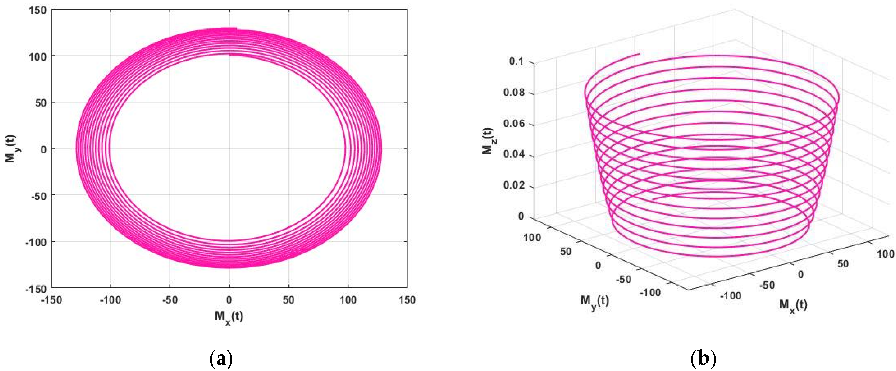
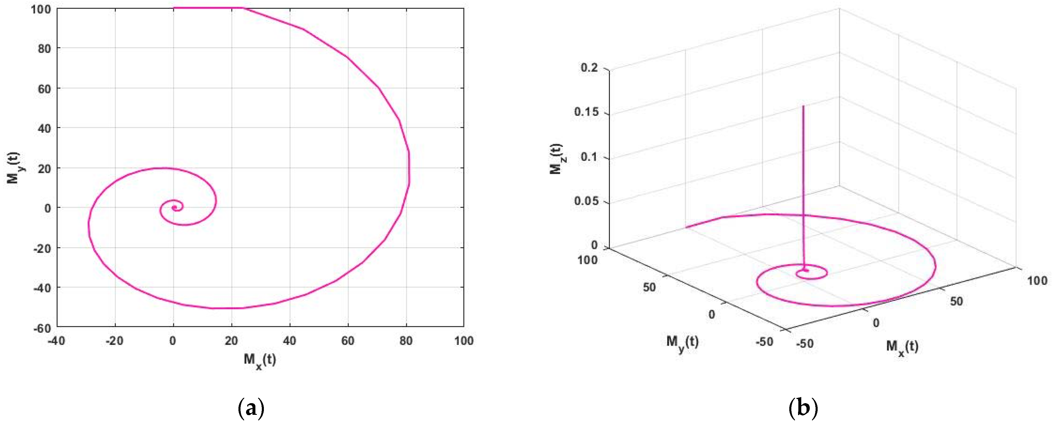
The approximate solution of the FNMRF system of equations is illustrated in Figure 1 for $T_{sim}=0.1 \mathrm{s}$. In Figure 1a,b we examine a limit cycle and plot a spiral, respectively. For $\alpha =\beta =\eta =1.03165$, we obtain the border of critical stability.

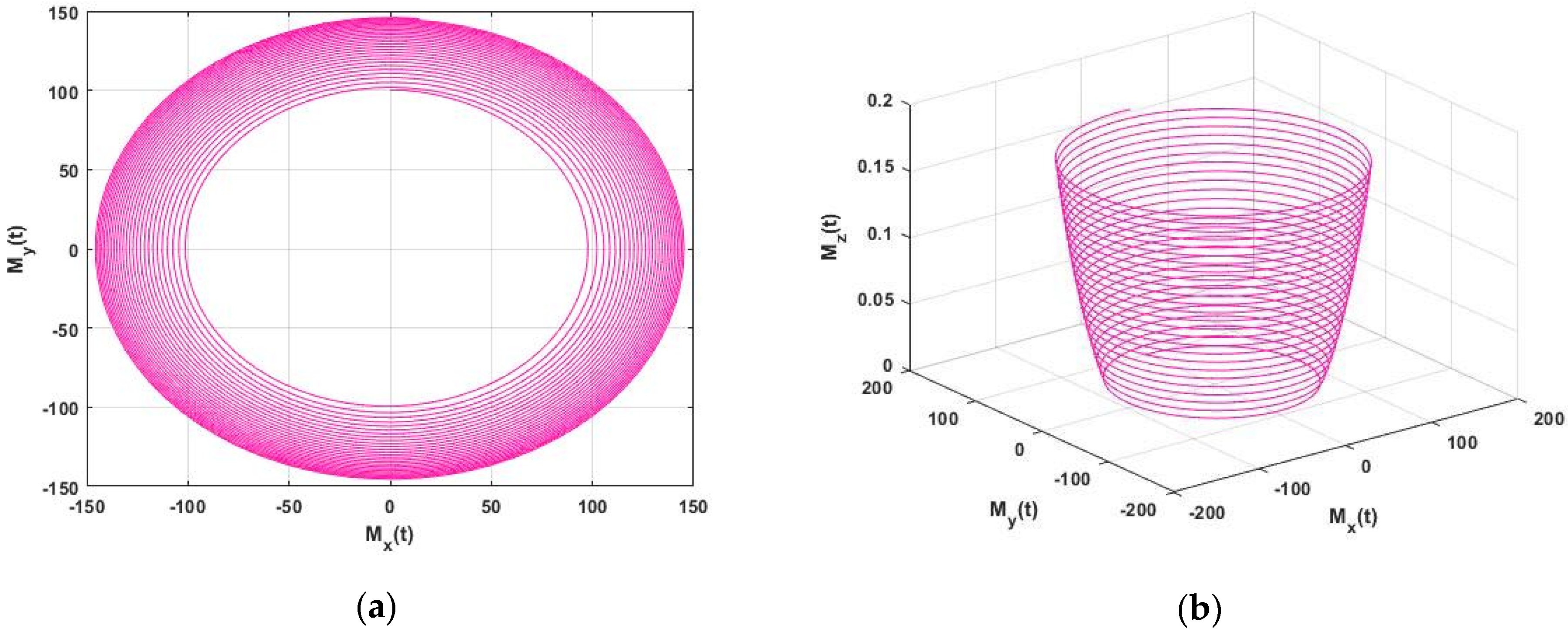
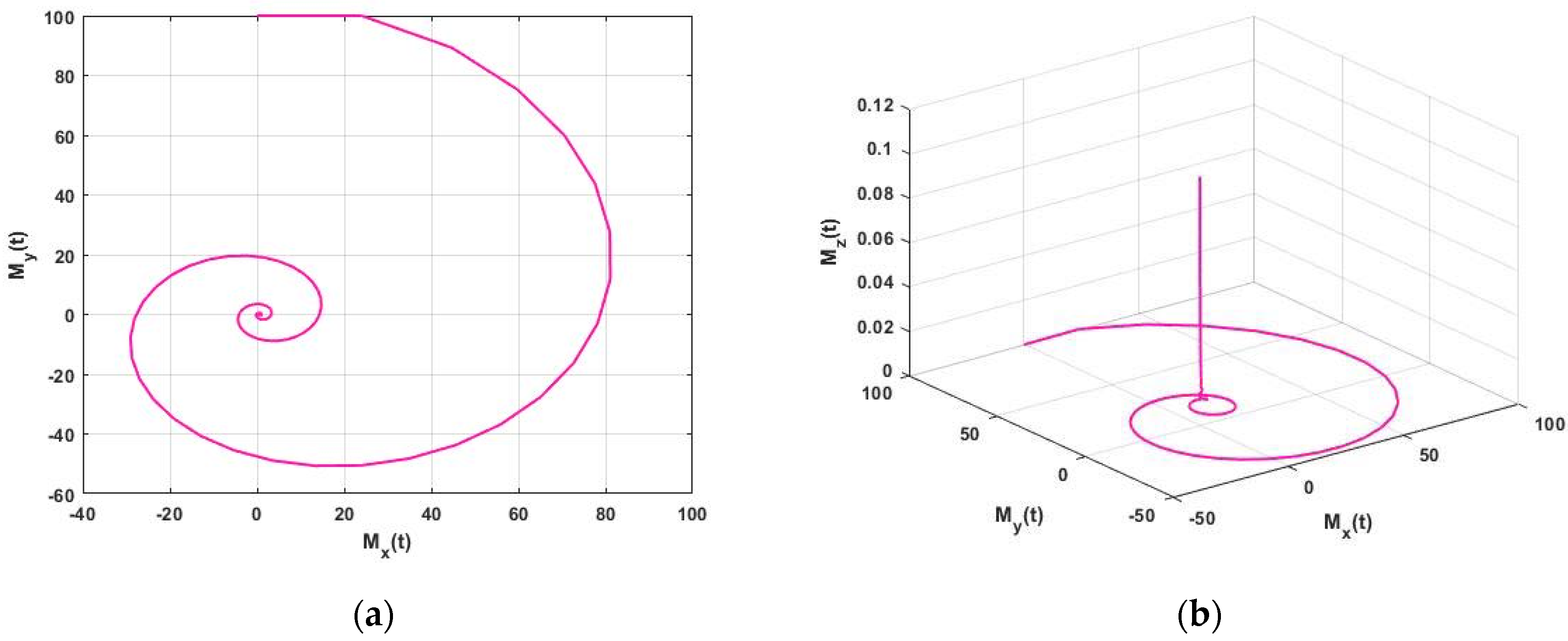
The approximate solution of the FNMRF system of equations is illustrated in Figure 2 for $T_{sim}=0.2 \mathrm{s}$ with parameters $\alpha =\beta =\eta =1.03165,T_2^{\prime }=20\hspace{0.17em}{\left(\mathrm{ms}\right)}^{\alpha },f_0=160 \mathrm{Hz},\hspace{0.17em}{T}_1^{\prime }=1 {\left(\mathrm{s}\right)}^{\alpha }$ with initial condition $\left(M_x\left(0\right),M_y\left(0\right),M_z\left(0\right)\right)=\left(0,100,0\right)$ for $T_{sim}=0.2 \mathrm{s}$.

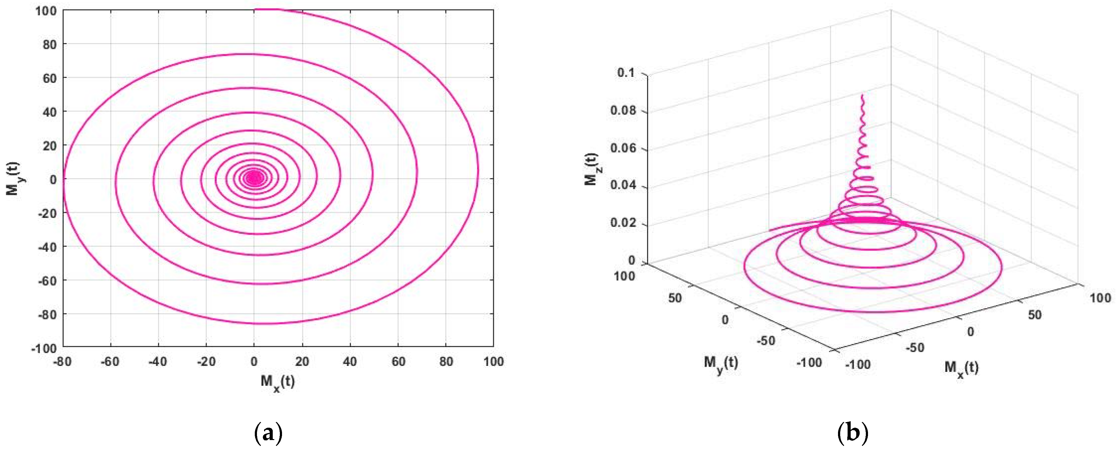
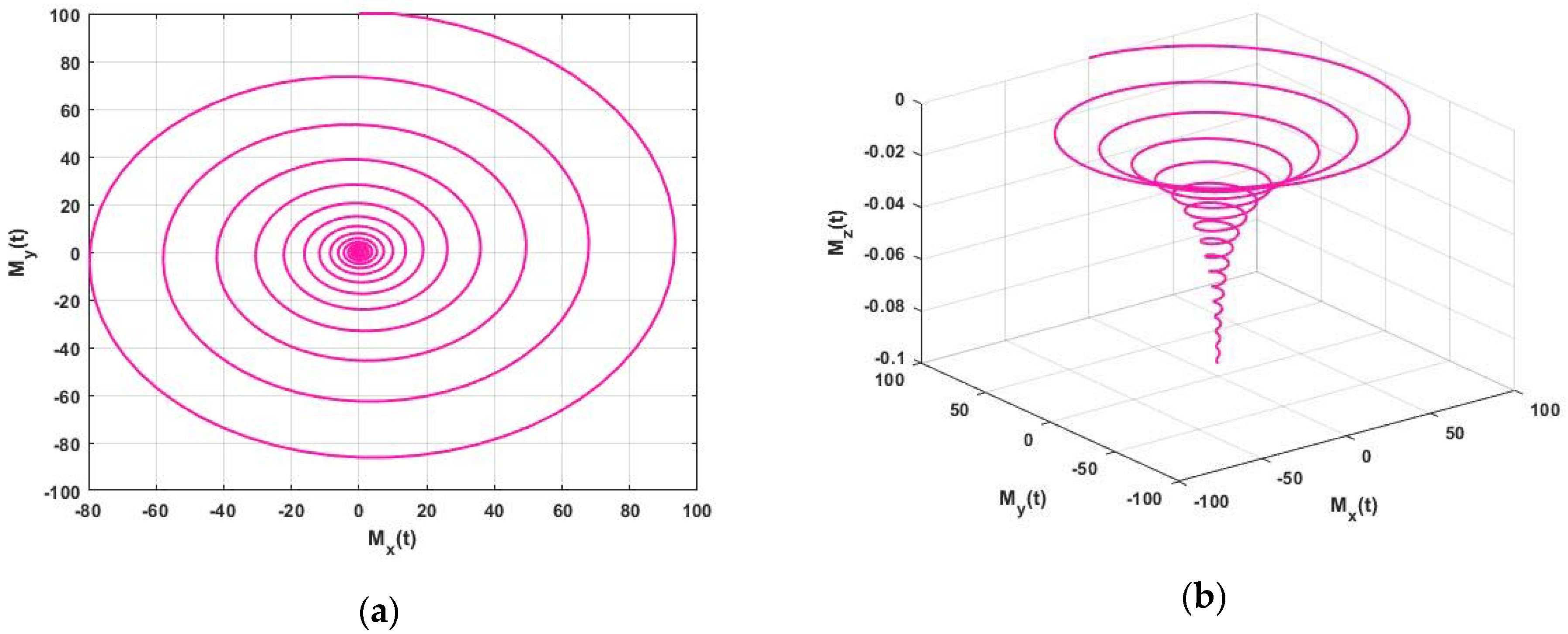
Figure 2a,b shows a limit cycle and a spiral plot for $T_{sim}=0.2 \mathrm{s}$. In this case, where we consider $\alpha =\beta =\eta =1.03163$ in Equation (4), we have the FNMRF system of equations, and the approximate solution is presented in Figure 3 for $T_{sim}=1 \mathrm{s}$. The solution of the FNMRF system with parameters $\alpha =\beta =\eta =1.0,$ $T_2^{\prime }=20\hspace{0.17em}{\left(\mathrm{ms}\right)}^{\overline{\mathsf{\alpha }}},f_0=160 \mathrm{Hz},\hspace{0.17em}{T}_1^{\prime }=1{\left( \mathrm{s}\right)}^{\overline{\mathsf{\alpha }}}$, and initial condition $\left(M_x\left(0\right),M_y\left(0\right),M_z\left(0\right)\right)=\left(0,100,0\right)$ for $T_{sim}=0.1 \mathrm{s}$ is depicted in Figure 4 for $M_0=1$ and in Figure 5 for $M_0=-1$. When we consider $\alpha =\beta =\eta =0.9$ in Equation (4), we have the FNMRF model, and the approximate solution is shown in Figure 6 with parameters $\alpha =\beta =\eta =0.9$, $T_2^{\prime }=20\hspace{0.17em}{\left(\mathrm{ms}\right)}^{\overline{\mathsf{\alpha }}},f_0=160 \mathrm{Hz},\hspace{0.17em}{\mathrm{T}}_1^{\prime }=1{\left(\mathrm{s}\right)}^{\overline{\mathsf{\alpha }}}$ with initial condition $\left(M_x\left(0\right),M_y\left(0\right),M_z\left(0\right)\right)=\left(0,100,0\right)$ for $T_{sim}=0.2 \mathrm{s}$ When we consider $\alpha =0.8, \beta =1,\eta =0.9$, $T_2^{\prime }=20\hspace{0.17em}{\left(\mathrm{ms}\right)}^{\overline{\mathsf{\alpha }}},f_0=160 \mathrm{Hz},\hspace{0.17em}{T}_1^{\prime }=1{\left(\mathrm{s}\right)}^{\overline{\mathsf{\alpha }}}$ and initial condition $\left(M_x\left(0\right),M_y\left(0\right),M_z\left(0\right)\right)=\left(0,100,0\right)$ in Equation (4), we have the FNMRF system of Equation (5) and the approximate solution obtained by MATHEMATICA for the $T_{sim}=0.1 \mathrm{s}$ is represented in Figure 7.

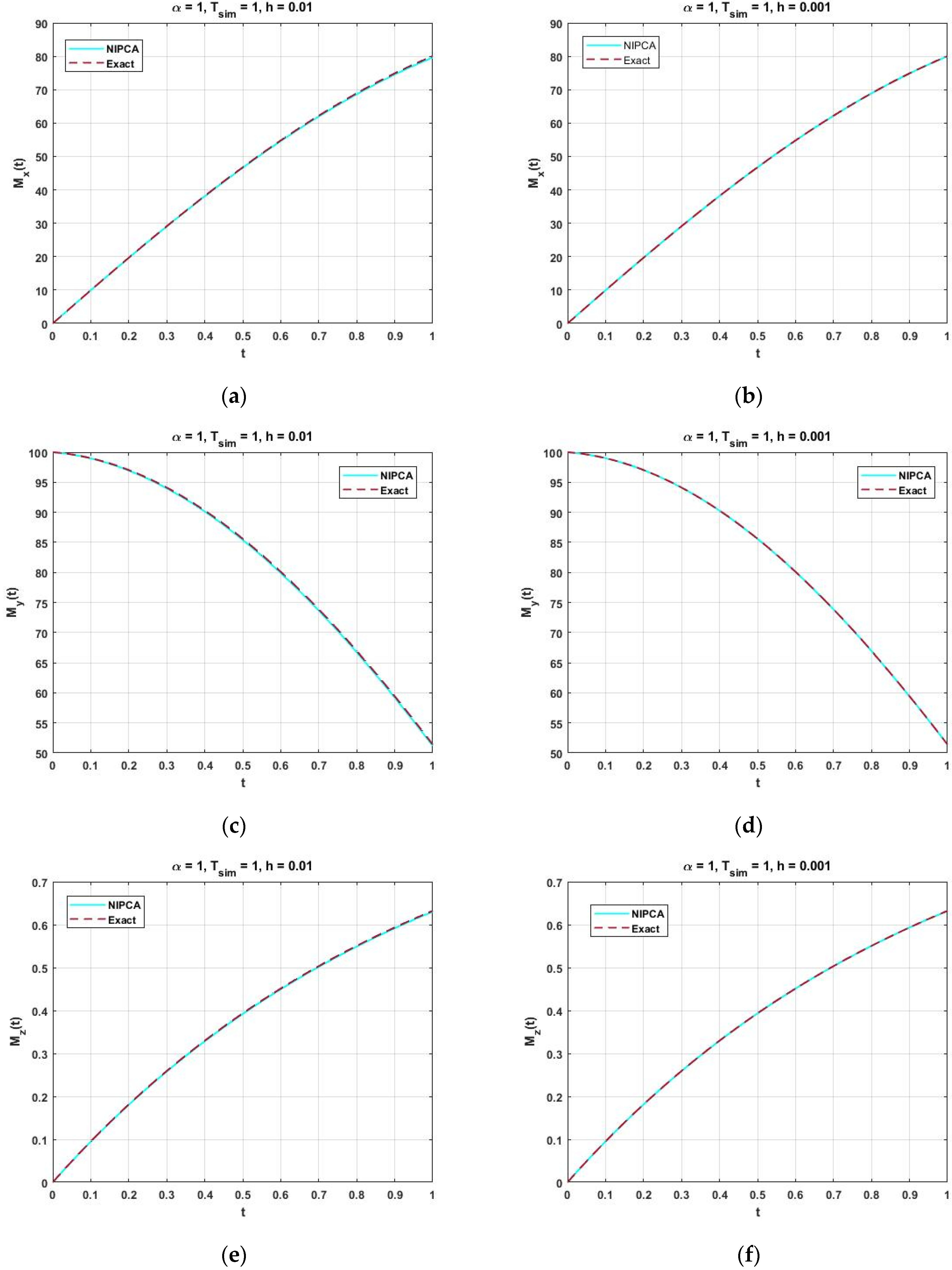
Figure 8 represents the comparison between the approximate solution and the analytical solution of the fractional FNMRF system for $M_x\left(t\right),\hspace{0.17em}\hspace{0.17em}{M}_y\left(t\right)$ and $M_z\left(t\right)$, respectively [23,24], for height steps $h=0.01$ and $h=0.001$.

We can see an excellent consistency of the solution and a similar result may also be detected for $M_z\left(t\right)$; see

Table 1. Average absolute error in the New Iterative Predictor-Corrector Algorithm (NIPCA).

$\mathrm{Simulation} \mathrm{Time} T_{sim}$	Components of M	$h=0.1$	$h=0.01$	$h=0.001$	$h=0.05$	$h=0.005$
$T_{sim}=0.1$	$M_x$	2.074 × 10−2	2.776 × 10−3	3.995 × 10−4	6.210 × 10−3	1.713 × 10−3
	$M_y$	2.485 × 10−1	1.658 × 10−2	2.369 × 10−3	4.200 × 10−2	1.009 × 10−2
	$M_z$	1.880 × 10−5	1.910 × 10−4	2.292 × 10−5	3.963 × 10−4	1.057 × 10−4
$T_{sim}=0.5$	$M_x$	1.705 × 10−1	4.708 × 10−2	5.090 × 10−3	1.573 × 10−1	2.460 × 10−2
	$M_y$	5.674 × 10−1	1.027 × 10−2	1.102 × 10−2	3.818 × 10−1	5.339 × 10−2
	$M_z$	5.963 × 10−3	8.645 × 10−5	8.983 × 10−5	3.657 × 10−3	4.415 × 10−4
$T_{sim}=1.0$	$M_x$	1.003 × 10−1	1.562 × 10−1	1.625 × 10−2	6.476 × 10−1	7.985 × 10−2
	$M_y$	1.257 × 10−1	1.638 × 10−1	1.694 × 10−2	7.152 × 10−1	8.342 × 10−2
	$M_z$	1.065 × 10−2	1.292 × 10−3	4.318 × 10−4	5.922 × 10−3	6.533 × 10−4

. From these observations, we conclude that the approximate solution well matches the analytical solution. The condition of stability for equation orders $\alpha =0.8, \beta =1,\eta =0.9$ of the solution is described in Figure 7.

Figure 1, Figure 2, Figure 3, Figure 4, Figure 5, Figure 6 and Figure 7, in 2D and 3D, illustrate the dynamics between $M_x\left(t\right)$, $M_y\left(t\right)$, and $M_z\left(t\right)$. For both cases, magnetization of the entire trajectory is presented in 3D with the starting point $\left(M_x\left(0\right),M_y\left(0\right),M_z\left(0\right)\right)=\left(0,100,0\right)$ and the return to its equilibrium value of $M_0$.

Figure 8 shows the exact solution and the numerical solution obtained by applying the presented NIPCA method for (a) $h=0.01$ and (b) $h=0.001$, and initial condition $\left(M_x\left(0\right),M_y\left(0\right),M_z\left(0\right)\right)=\left(0,100,0\right)$ for $T_{sim}=1 \mathrm{s}$. The maximum error in $\left(M_x,M_y,M_z\right)$ and simulation time $T_{sim}=0.1 \mathrm{s}, 0.5 \mathrm{s} \mathrm{and} 1.0 \mathrm{s}$ with time steps $h=0.1, 0.01, 0.001, 0.05, \mathrm{and} 0.005$ are listed in Table 1. It is easily shown from Table 1 that the time step is directly proportional to the error.

5. Conclusions

In this article, we obtained nonlinear fractional nuclear magnetic resonance flow equations (FNMRFEs) and the New Iterative Predictor-Corrector Algorithm (NIPCA) for their approximate solution. For NMR, the developed mathematical model allows the description and investigation of magnetization for spin dynamics (relaxation times $T_1^{\prime } \mathrm{and} T_2^{\prime }$) at the resonance frequency ${\varpi }_{0 }^{\prime }$ in a static magnetic field $B_0$. A New Iterative Predictor-Corrector Algorithm (NIPCA) was proposed to solve nonlinear fractional nuclear magnetic resonance flow equations. The time efficiency and high accuracy of the proposed technique are evident from the detailed error analysis of the FNMRFEs.

References

- Singh, H.; Srivastava, H.M. Numerical Simulation for Fractional-Order Bloch Equation Arising in Nuclear Magnetic Resonance by Using the Jacobi Polynomials. Appl. Sci. 2020, 10, 2850. [Google Scholar] [CrossRef] [Green Version]
- Johnston, E.R. Solution of the Bloch Equations including Relaxation. Concepts Magn. Reson. Part A 2020, 2020, 1–5. [Google Scholar] [CrossRef]
- Ali, H.M. An efficient approximate-analytical method to solve time-fractional KdV and KdVB equations. Inf. Sci. Lett. 2020, 9, 189–198. [Google Scholar]
- Sultana, M.; Arshad, U.; Alam, N.; Bazighifan, O.; Askar, S.; Awrejcewicz, J. New Results of the Time-Space Fractional Derivatives of Kortewege-De Vries Equations via Novel Analytic Method. Symmetry 2021, 13, 2296. [Google Scholar] [CrossRef]
- Zada, L.; Al-Hamami, M.; Nawaz, R.; Jehanzeb, S.; Morsy, A.; Abdel-Aty, A.; Nisar, K.S. A New Approach for Solving Fredholm Integro-Differential Equations. Inf. Sci. Lett. 2021, 10, 407–415. [Google Scholar]
- Khater, M.M.A.; Attia, R.A.M.; Abdel-Aty, A.H. Computational analysis of a nonlinear fractional emerging telecommunication model with higher-order dispersive cubic-quintic. Inf. Sci. Lett. 2020, 9, 83–93. [Google Scholar]
- Mohammadein, S.A.; Gad El-Rab, R.A.; Ali, M.S. The Simplest Analytical Solution of Navier-Stokes Equations. Inf. Sci. Lett. 2021, 10, 159–165. [Google Scholar]
- Abragam, A. Principles of Nuclear Magnetism; Oxford University Press: New York, NY, USA, 2002. [Google Scholar]
- Brown, R.W.; Cheng, Y.C.N.; Haacke, E.M.; Thompson, M.R.; Venkatesan, R. Magnetic Resonance Imaging: Physical Principles and Sequence Design; John Wiley and Sons: New York, NY, USA, 2014; ISBN 978-0-471-72085-0. [Google Scholar]
- Singh, H. A new numerical algorithm for fractional model of Bloch equation in nuclear magnetic resonance. Alex. Eng. J. 2016, 55, 2863–2869. [Google Scholar] [CrossRef] [Green Version]
- Caputo, M. Linear Models of Dissipation whose Q is almost Frequency Independent-II. Geophys. J. Int. 1967, 13, 529–539. [Google Scholar] [CrossRef]
- Daftardar-Gejji, V.; Jafari, H. Adomian decomposition: A tool for solving a system of fractional differential equations. J. Math. Anal. Appl. 2005, 301, 508–518. [Google Scholar] [CrossRef] [Green Version]
- Adomian, G. A review of decomposition method in applied mathematics. J. Math. Anal. Appl. 1988, 135, 501–544. [Google Scholar] [CrossRef] [Green Version]
- Hemeda, A.A. Homotopy perturbation method for solving systems of nonlinear coupled equations. Appl. Math. Sci. 2012, 6, 4787–4800. [Google Scholar]
- Bhalekar, S.; Daftardar-Gejji, V. Convergence of the new iterative method. Int. J. Differ. Equ. 2011, 2011, 1–10. [Google Scholar] [CrossRef]
- Bhalekar, S.; Daftardar-Gejji, V. Solving a system of nonlinear functional equations using a revised new iterative method. Int. J. Math. Comput. Sci. 2012, 6, 968–972. [Google Scholar] [CrossRef]
- Saeed, R.K.; Aziz, K.M. An iterative method with quartic convergence for solving nonlinear equations. Appl. Math. Comput. 2008, 202, 435–440. [Google Scholar] [CrossRef]
- Daftardar-Gejji, V.; Jafari, H. An iterative method for solving nonlinear functional equations. J. Math. Anal. Appl. 2006, 316, 753–763. [Google Scholar] [CrossRef] [Green Version]
- Khalid, M.; Sultana, M.; Arshad, U.; Shoaib, M. A Comparison between New Iterative Solutions of Nonlinear Oscillator Equation. Int. J. Comput. Appl. 2015, 128, 1–5. [Google Scholar] [CrossRef]
- Khalid, M.; Sultana, M.; Zaidi, F.; Arshad, U. Solving Linear and Nonlinear Klein-Gordon Equations by New Perturbation Iteration Transform Method. TWMS J. App. Eng. Math. 2016, 6, 115–125. [Google Scholar]
- Khalid, M.; Sultana, M.; Zaidi, F.; Arshad, U. An Effective Perturbation Iteration Algorithm for Solving Riccati Differential Equations. Int. J. Comput. Appl. 2015, 111, 0975–8887. [Google Scholar] [CrossRef]
- Daftardar-Gejji, V.; Sukale, Y.; Bhalekar, S. A new predictor-corrector method for fractional differential equations. Appl. Math. Comput. 2014, 244, 158–182. [Google Scholar] [CrossRef]
- Khalid, M.; Sultana, M.; Arshad, U. Procuring Analytical Solution of Nonlinear Nuclear Magnetic Resonance Model of Fraction Order. Sohag J. Math. 2017, 4, 69–73. [Google Scholar] [CrossRef]
- Petráš, I. Modeling and numerical analysis of fractional-order Bloch equations. Comput. Math. Appl. 2011, 61, 341–356. [Google Scholar] [CrossRef]
Figure 1.
Approximate solution (a) 2D Plot and (b) 3D Plot of the FNMRF system for , and initial condition for .
Figure 2.
Approximate solution (a) 2D Plot and (b) 3D Plot of the FNMRF system for and initial condition for .
Figure 3.
Figure 4.
Figure 5.
Figure 6.
Figure 7.
Figure 8.
Comparison between the Exact solution and Analytical solution of the FNMRF system for (a) (b) h = 0.001 (c) h = 0.01 (d) h = 0.001 (e) h = 0.01 (f) h = 0.001 and initial condition for .