The Mittag–Leffler Functions for a Class of First-Order Fractional Initial Value Problems: Dual Solution via Riemann–Liouville Fractional Derivative

Abstract

In this paper, a new approach is developed to solve a class of first-order fractional initial value problems. The present class is of practical interest in engineering science. The results are based on the Riemann–Liouville fractional derivative. It is shown that the dual solution can be determined for the considered class. The first solution is obtained by means of the Laplace transform and expressed in terms of the Mittag–Leffler functions. The second solution was determined through a newly developed approach and given in terms of exponential and trigonometric functions. Moreover, the results reduce to the ordinary version as the fractional-order tends to unity. Characteristics of the dual solution are discussed in detail. Furthermore, the advantages of the second solution over the first one is declared. It is revealed that the second solution is real at certain values of the fractional-order. Such values are derived theoretically and accordingly, and the behavior of the real solution is shown through several plots. The present analysis may be introduced for obtaining the solution in a straightforward manner for the first time. The developed approach can be further extended to include higher-order fractional initial value problems of oscillatory types.

1. Introduction

The fractional calculus (FC) is a growing field of research that is usually utilized to investigate the physical phenomena of the memory effect [1,2,3]. Many scientific models have been analyzed via the FC approach [4,5,6,7,8]. A comprehensive list of FC applications are listed in Refs. [9,10,11,12,13,14]. For example, the fractional physical model of the projectile motion was discussed by Ebaid [15] and Ebaid et al. [16] utilizing the Caputo fractional derivative (CFD), and their results have been compared with experimental data. In addition, Ahmed et al. [17] implemented the Riemann–Liouville fractional derivative (RLFD) to analyze the same problem. The above models have been formulated in the form of second-order fractional initial value problems (2nd-order FIVPs).

Furthermore, Kumar et al. [18] and Ebaid et al. [19] studied the first-order fractional initial value problems (1st-order FIVPs) describing the absorption of light by the interstellar matter (called Ambartsumian-fractional model) by means of CFD. The exact solution of this model was determined by Ebaid et al. [19] using the Laplace transform (LT). Moreover, the RLFD was used by El-Zahar et al. [20] to provide the solution of the Ambartsumian-fractional model in a closed series form. Recent interesting results and applications of FC can be found in [21,22,23,24,25,26,27,28,29]. Very recently, El-Dib and Elgazery [30] investigated the nonlinear oscillations utilizing the properties of the RLFD.

The objective of this work is to extend the application of RLFD to a certain class of 1st-order FIVPs of oscillatory nature. Such class is of great importance in the field of engineering. Thus, this paper considers the class of 1st-order FIVPs:

$${}_{-\infty }^{RL}{D}_t^{\alpha }y\left(t\right)+{\omega }^{2}y\left(t\right)=acos\left(\mathrm{\Omega }t\right),D_t^{\alpha -1}y\left(0\right)=A,0<\alpha \le 1,$$

(1)

where $\alpha$ is the non-integer order of the RLFD, while a, $\omega$, $\mathrm{\Omega }$, and A are constants. Moreover, the present model can be viewed as a forced harmonic-oscillator of the first-order in a fractional form, and it may be of practical interest in engineering science. Although Equation (1) seems simple, obtaining its exact solution is not an easy task due to several factors that will be illustrated. It will also be shown that a dual solution exists. As a solution method, the LT is a basic and effective tool to solve 1st-order FIVPs, even for higher-order FIVPs. The LT will be applied on the current class to construct the first solution in terms of Mittag–Leffler functions. However, a new approach is to be developed in this paper to determine the second solution in which only exponential and trigonometric functions are involved.

Characteristics of these solutions will also be discussed. The advantages of the second solution over the first one will be demonstrated. To our knowledge, the present analysis has not been yet reported in the literature. The rest of the paper is organized as follows. In Section 2, the definition/properties of the RLFD and the Mittag–Leffler functions are introduced. In Section 3, a basic theorem for the particular solution of Equation (1) is introduced. Moreover, it is shown that the present particular solution reduces to the corresponding one in the literature as a special case. In Section 4, the dual solution of 1st-order FIVPs (1) is constructed and analyzed in detail. Section 5 is devoted to studying the characteristics of the established solutions. In addition, the $\alpha$-values that admit real solutions of the present class are obtained theoretically. Moreover, the behavior of the current solution is discussed. In Section 6, the main conclusions are summarized.

2. Preliminaries

The Riemann–Liouville fractional integral of order $\alpha$ of function $f:[c,d]\to \mathbb{R}(-\infty <c<d<\infty )$ is defined as [1,2,3]

$${}_c{I}_t^{\alpha }f\left(t\right)=\frac{1}{\mathsf{\Gamma }\left(\alpha \right)}{\int }_c^t\frac{f\left(\tau \right)}{{(t-\tau )}^{1-\alpha }}d\tau ,t>c,\alpha >0.$$

(2)

The RLFD of order $\alpha \in {\mathbb{R}}_0^{+}$ is [1,2,3]

$${}_c^{RL}{D}_t^{\alpha }f\left(t\right)=\frac{1}{\mathsf{\Gamma }\left(n-\alpha \right)}\frac{d^n}{d{t}^n}\left({\int }_c^t\frac{f\left(\tau \right)}{{\left(t-\tau \right)}^{\alpha -n+1}}d\tau \right),n=\left[\alpha \right]+1,t>c,$$

(3)

where $\left[\alpha \right]$ means the integral part of $\alpha$. For $t\in \mathbb{R}$ and $c\to -\infty$, the RLFD of the functions $e^{i\omega t}$, $cos\left(\omega t\right)$, and $sin\left(\omega t\right)$ are [30,31]

$$\begin{array}{cc}& {}_{-\infty }^{RL}{D}_t^{\alpha }{e}^{i\omega t}={\left(i\omega \right)}^{\alpha }{e}^{i\omega t},\hfill \\ & {}_{-\infty }^{RL}{D}_t^{\alpha }cos\left(\omega t\right)={\omega }^{\alpha }cos\left(\omega t+\frac{\alpha \pi }{2}\right),\hfill \\ & {}_{-\infty }^{RL}{D}_t^{\alpha }sin\left(\omega t\right)={\omega }^{\alpha }sin\left(\omega t+\frac{\alpha \pi }{2}\right).\hfill \end{array}$$

(4)

It may be important to mention that the first equation in (4) was implemented by El-Dib and Elgazery [30]. Such implementation is based on the proof introduced by Ortigueira et al. [31]. However, the last two equations in (4) are utilized in [30] without proof, which may be because the authors [30] considered the derivation of these equations an easy task. For this reason, the proof and validity of the last two equations in (4) are provided in the Appendix A. The Laplace transform (LT) of the RLFD, as $c\to 0$, is

$$\mathcal{L}\left[{}_0^{RL}{D}_t^{\alpha }y\left(t\right)\right]=s^{\alpha }Y\left(s\right)-\sum _{i=0}^{n-1}{s}^i{D}_t^{\alpha -i-1}y\left(0\right).$$

(5)

In view of Equations (4) and (5), we have to distinguish between the properties of the RLFD when $c\to -\infty$ and $c\to 0$, i.e., ${}_{-\infty }^{RL}{D}_t^{\alpha }$ and ${}_0^{RL}{D}_t^{\alpha }$, respectively. Thus, the dual solution of Equation (1) is expected.

The Mittag–Leffler function of two parameters is defined by

$$E_{\alpha ,\gamma }\left(z\right)=\sum _{i=0}^{\infty }\frac{z^i}{\mathsf{\Gamma }(\alpha i+\gamma )},(\alpha >0,\gamma >0).$$

(6)

In particular, we have the following properties

$$E_{\alpha ,1}\left(z\right)=E_{\alpha }\left(z\right),E_1\left(z\right)=e^z,E_{2,1}(-z^2)=cos\left(z\right),E_{2,2}(-z^2)=\frac{sinz}{z}.$$

(7)

The inverse LT of some expressions can be given via the Mittag–Leffler function as

$${\mathcal{L}}^{-1}\left(\frac{s^{\alpha -\gamma }}{s^{\alpha }+{\omega }^2}\right)=t^{\gamma -1}{E}_{\alpha ,\gamma }(-{\omega }^2{t}^{\alpha }),Re\left(s\right)>{\left|{\omega }^2\right|}^{\frac{1}{\alpha }},$$

(8)

which gives the equalities:

$$\begin{array}{ccc}& & {\mathcal{L}}^{-1}\left(\frac{s^{\alpha -1}}{s^{\alpha }+1}\right)=E_{\alpha }(-t^{\alpha }),\hfill \end{array}$$

(9)

$$\begin{array}{ccc}& & {\mathcal{L}}^{-1}\left(\frac{1}{s^{\alpha }+{\omega }^2}\right)=t^{\alpha -1}{E}_{\alpha ,\alpha }(-{\omega }^2{t}^{\alpha }),Re\left(s\right)>{\left|{\omega }^2\right|}^{\frac{1}{\alpha }},\hfill \end{array}$$

(10)

$$\begin{array}{ccc}& & {\mathcal{L}}^{-1}\left(\frac{s^{-1}}{s^{\alpha }+{\omega }^2}\right)=t^{\alpha }{E}_{\alpha ,\alpha +1}(-{\omega }^2{t}^{\alpha }),Re\left(s\right)>{\left|{\omega }^2\right|}^{\frac{1}{\alpha }}.\hfill \end{array}$$

(11)

3. Analysis

Theorem 1

(The particular solution).The particular solution $y_p\left(t\right)$ of Equation (1) is given by

$$y_p\left(t\right)={\rho }_1\left(\alpha \right)cos\left(\mathrm{\Omega }t\right)+{\rho }_2\left(\alpha \right)sin\left(\mathrm{\Omega }t\right),0<\alpha \le 1,$$

(12)

where ${\rho }_1\left(\alpha \right)$ and ${\rho }_2\left(\alpha \right)$ are

$${\rho }_1\left(\alpha \right)=a\left(\frac{{\omega }^2+{\mathrm{\Omega }}^{\alpha }cos\left(\frac{\pi \alpha }{2}\right)}{{\omega }^4+{\mathrm{\Omega }}^{2\alpha }+2{\omega }^2{\mathrm{\Omega }}^{\alpha }cos\left(\frac{\pi \alpha }{2}\right)}\right),{\rho }_2\left(\alpha \right)=a\left(\frac{{\mathrm{\Omega }}^{\alpha }sin\left(\frac{\pi \alpha }{2}\right)}{{\omega }^4+{\mathrm{\Omega }}^{2\alpha }+2{\omega }^2{\mathrm{\Omega }}^{\alpha }cos\left(\frac{\pi \alpha }{2}\right)}\right).$$

(13)

Proof. 

Assume $y_p$ in the form of Equation (12), then

$$\begin{array}{cc}\hfill {}_{-\infty }^{RL}{D}_t^{\alpha }{y}_p=& {\rho }_1\left(\alpha \right){}_{-\infty }^{RL}{D}_t^{\alpha }cos\left(\mathrm{\Omega }t\right)+{\rho }_2\left(\alpha \right){}_{-\infty }^{RL}{D}_t^{\alpha }sin\left(\mathrm{\Omega }t\right),\hfill \\ \hfill & ={\mathrm{\Omega }}^{\alpha }cos\left(\mathrm{\Omega }t\right)\left({\rho }_1\left(\alpha \right)cos\left(\frac{\pi \alpha }{2}\right)+{\rho }_2\left(\alpha \right)sin\left(\frac{\pi \alpha }{2}\right)\right)+\hfill \\ \hfill & {\mathrm{\Omega }}^{\alpha }sin\left(\mathrm{\Omega }t\right)\left({\rho }_2\left(\alpha \right)cos\left(\frac{\pi \alpha }{2}\right)-{\rho }_1\left(\alpha \right)sin\left(\frac{\pi \alpha }{2}\right)\right),\hfill \end{array}$$

(14)

and hence

$$\begin{array}{cc}\hfill {}_{-\infty }^{RL}{D}_t^{\alpha }{y}_p+{\omega }^2{y}_p=& \left[\left({\mathrm{\Omega }}^{\alpha }cos\left(\frac{\pi \alpha }{2}\right)+{\omega }^2\right){\rho }_1\left(\alpha \right)+{\mathrm{\Omega }}^{\alpha }sin\left(\frac{\pi \alpha }{2}\right){\rho }_2\left(\alpha \right)\right]cos\left(\mathrm{\Omega }t\right)+\hfill \\ \hfill & \left[\left({\mathrm{\Omega }}^{\alpha }cos\left(\frac{\pi \alpha }{2}\right)+{\omega }^2\right){\rho }_2\left(\alpha \right)-{\mathrm{\Omega }}^{\alpha }sin\left(\frac{\pi \alpha }{2}\right){\rho }_1\left(\alpha \right)\right]sin\left(\mathrm{\Omega }t\right).\hfill \end{array}$$

(15)

Substituting Equation (15) into Equation (1), we obtain the algebraic system:

$$\begin{array}{cc}& \left({\mathrm{\Omega }}^{\alpha }cos\left(\frac{\pi \alpha }{2}\right)+{\omega }^2\right){\rho }_1\left(\alpha \right)+{\mathrm{\Omega }}^{\alpha }sin\left(\frac{\pi \alpha }{2}\right){\rho }_2\left(\alpha \right)=a,\hfill \\ & \left({\mathrm{\Omega }}^{\alpha }cos\left(\frac{\pi \alpha }{2}\right)+{\omega }^2\right){\rho }_2\left(\alpha \right)-{\mathrm{\Omega }}^{\alpha }sin\left(\frac{\pi \alpha }{2}\right){\rho }_1\left(\alpha \right)=0.\hfill \end{array}$$

(16)

Solving the algebraic system (16) for ${\rho }_1\left(\alpha \right)$ and ${\rho }_2\left(\alpha \right)$, we obtain

$${\rho }_1\left(\alpha \right)=a\left(\frac{{\omega }^2+{\mathrm{\Omega }}^{\alpha }cos\left(\frac{\pi \alpha }{2}\right)}{{\omega }^4+{\mathrm{\Omega }}^{2\alpha }+2{\omega }^2{\mathrm{\Omega }}^{\alpha }cos\left(\frac{\pi \alpha }{2}\right)}\right),{\rho }_2\left(\alpha \right)=a\left(\frac{{\mathrm{\Omega }}^{\alpha }sin\left(\frac{\pi \alpha }{2}\right)}{{\omega }^4+{\mathrm{\Omega }}^{2\alpha }+2{\omega }^2{\mathrm{\Omega }}^{\alpha }cos\left(\frac{\pi \alpha }{2}\right)}\right).$$

(17)

Inserting (17) into (12) and simplifying, we obtain $y_p$ in the form:

$$y_p\left(t\right)=a\left(\frac{{\omega }^{2}cos\left(\mathrm{\Omega }t\right)+{\mathrm{\Omega }}^{\alpha }cos\left(\mathrm{\Omega }t-\frac{\pi \alpha }{2}\right)}{{\omega }^4+{\mathrm{\Omega }}^{2\alpha }+2{\omega }^2{\mathrm{\Omega }}^{\alpha }cos\left(\frac{\pi \alpha }{2}\right)}\right),$$

(18)

which completes the proof. □

Lemma 1.

At $a=1$, the particular solution $y_p\left(t\right)$ of Equation (1) reduces to

$$y_p\left(t\right)=\frac{{\omega }^{2}cos\left(\mathrm{\Omega }t\right)+{\mathrm{\Omega }}^{\alpha }cos\left(\mathrm{\Omega }t-\frac{\pi \alpha }{2}\right)}{{\omega }^4+{\mathrm{\Omega }}^{2\alpha }+2{\omega }^2{\mathrm{\Omega }}^{\alpha }cos\left(\frac{\pi \alpha }{2}\right)}.$$

(19)

Proof. 

The proof follows immediately by setting $a=1$ in Equation (18); thus

$$y_p\left(t\right)=\frac{{\omega }^{2}cos\left(\mathrm{\Omega }t\right)+{\mathrm{\Omega }}^{\alpha }cos\left(\mathrm{\Omega }t-\frac{\pi \alpha }{2}\right)}{{\omega }^4+{\mathrm{\Omega }}^{2\alpha }+2{\omega }^2{\mathrm{\Omega }}^{\alpha }cos\left(\frac{\pi \alpha }{2}\right)},$$

(20)

which agrees with the obtained particular integral in Ref. [30] (Equation (7)) using the ${\left(D^{\alpha }+{\omega }^2\right)}^{-1}$ operator. However, our approach is straightforward and easier. □

4. Dual Solution

It is shown in this section that the dual solution of the present class of 1st-order FIVPs can be derived. The first solution is obtained in terms of Mittag–Leffler functions, while the second is provided in terms of exponential and trigonometric functions so that the Mittag–Leffler function can be avoided. Characteristics of these solutions will also be discussed in a subsequent section.

4.1. Solution in Terms of Mittag–Leffler Functions

Applying the LT on Equation (1), yields

$$s^{\alpha }Y\left(s\right)-D_t^{\alpha -1}y\left(0\right)+{\omega }^{2}Y\left(s\right)=\frac{as}{s^2+{\mathrm{\Omega }}^2},$$

(21)

where $Y\left(s\right)$ is the LT of $y\left(t\right)$. Solving (21) for $Y\left(s\right)$ gives

$$Y\left(s\right)=\frac{A}{s^{\alpha }+{\omega }^2}+\frac{as}{(s^{\alpha }+{\omega }^2)(s^2+{\mathrm{\Omega }}^2)}.$$

(22)

The solution $y\left(t\right)$ is obtained by applying the inverse LT on $Y\left(s\right)$, this gives

$$y\left(t\right)=A{\mathcal{L}}^{-1}\left(\frac{1}{s^{\alpha }+{\omega }^2}\right)+{\mathcal{L}}^{-1}\left[\frac{as}{(s^{\alpha }+{\omega }^2)(s^2+{\mathrm{\Omega }}^2)}\right],$$

(23)

i.e.,

$$y\left(t\right)=A{t}^{\alpha -1}{E}_{\alpha ,\alpha }\left(-{\omega }^2{t}^{\alpha }\right)+a{\mathcal{L}}^{-1}\left(\frac{1}{s^{\alpha }+{\omega }^2}\right)*{\mathcal{L}}^{-1}\left(\frac{s}{s^2+{\mathrm{\Omega }}^2}\right),$$

(24)

where $(*)$ refers to the convolution operation. Therefore

$$y\left(t\right)=A{t}^{\alpha -1}{E}_{\alpha ,\alpha }\left(-{\omega }^2{t}^{\alpha }\right)+a{\int }_0^t{\tau }^{\alpha -1}{E}_{\alpha ,\alpha }\left(-{\omega }^2{\tau }^{\alpha }\right)cos\left[\mathrm{\Omega }\left(t-\tau \right)\right]d\tau ,$$

(25)

which can be written as

$$\begin{array}{ccc}& & y\left(t\right)=A{t}^{\alpha -1}{E}_{\alpha ,\alpha }\left(-{\omega }^2{t}^{\alpha }\right)+acos\left(\mathrm{\Omega }t\right){\int }_0^t{\tau }^{\alpha -1}{E}_{\alpha ,\alpha }\left(-{\omega }^2{\tau }^{\alpha }\right)cos\left(\mathrm{\Omega }\tau \right)d\tau +\hfill \\ & & asin\left(\mathrm{\Omega }t\right){\int }_0^t{\tau }^{\alpha -1}{E}_{\alpha ,\alpha }\left(-{\omega }^2{\tau }^{\alpha }\right)sin\left(\mathrm{\Omega }\tau \right)d\tau ,\hfill \end{array}$$

(26)

As $\alpha \to 1$, the solution reduces to

$$\begin{array}{ccc}& & y\left(t\right)=A{E}_{1,1}\left(-{\omega }^{2}t\right)+acos\left(\mathrm{\Omega }t\right){\int }_0^t{E}_{1,1}\left(-{\omega }^2\tau \right)cos\left(\mathrm{\Omega }\tau \right)d\tau +\hfill \\ & & asin\left(\mathrm{\Omega }t\right){\int }_0^t{E}_{1,1}\left(-{\omega }^2\tau \right)sin\left(\mathrm{\Omega }\tau \right)d\tau ,\hfill \end{array}$$

(27)

i.e.,

$$y\left(t\right)=A{e}^{-{\omega }^{2}t}+acos\left(\mathrm{\Omega }t\right){\int }_0^t{e}^{-{\omega }^2\tau }cos\left(\mathrm{\Omega }\tau \right)d\tau +asin\left(\mathrm{\Omega }t\right){\int }_0^t{e}^{-{\omega }^2\tau }sin\left(\mathrm{\Omega }\tau \right)d\tau .$$

(28)

Evaluating the involved integrals and simplifying yields

$$y\left(t\right)=\left(A-\frac{a{\omega }^2}{{\omega }^4+{\mathrm{\Omega }}^2}\right)e^{-{\omega }^{2}t}+\frac{a}{{\omega }^4+{\mathrm{\Omega }}^2}\left[{\omega }^{2}cos\left(\mathrm{\Omega }t\right)+\mathrm{\Omega }sin\left(\mathrm{\Omega }t\right)\right],$$

(29)

which agrees with the solution of the ordinary version of the FIVP (1). However, the present solution in fractional form (26) is not analytic at $t=0,\forall \alpha \in (0,1)$ for the existence of term $t^{\alpha -1}$. This phenomena will be avoided in the next section via a new approach to obtaining the exact analytic solution for the FIVP (1) in terms of exponential and trigonometric functions. Equation (26) is non-analytic at $t=0$, which is just a consequence of applying the LT on the RLFD as c tends to zero. This gives the second solution, in terms of exponential and trigonometric functions, an advantage over the first one, in terms of the Mittag–Leffler functions.

4.2. Solution in Terms of Exponential and Trigonometric Functions

The general solution $y\left(t\right)$ of the FIVP (1) consists of the complementary solution $y_c\left(t\right)$ and the particular solution $y_p\left(t\right)$ so that

$$y\left(t\right)=y_c\left(t\right)+y_p\left(t\right),$$

(30)

where $y_p\left(t\right)$ was already obtained by Theorem 1, while $y_c\left(t\right)$ is the solution of the homogeneous part:

$${}_{-\infty }^{RL}{D}_t^{\alpha }{y}_c\left(t\right)+{\omega }^2{y}_c\left(t\right)=0.$$

(31)

Assume $y_c\left(t\right)$ is in the form:

$$y_c\left(t\right)=c_1\left(\alpha \right)cos\left(\delta t\right)+c_2\left(\alpha \right)sin\left(\delta t\right),$$

(32)

where $c_1\left(\alpha \right)$, $c_2\left(\alpha \right)$, and $\delta \left(\omega \right)$ are to be determined. Substituting (32) into (31), yields

$$\begin{array}{ccc}& & \left[\left({\delta }^{\alpha }cos\left(\frac{\pi \alpha }{2}\right)+{\omega }^2\right)c_1\left(\alpha \right)+{\delta }^{\alpha }sin\left(\frac{\pi \alpha }{2}\right)c_2\left(\alpha \right)\right]cos\left(\delta t\right)+\hfill \\ & & \left[\left({\delta }^{\alpha }cos\left(\frac{\pi \alpha }{2}\right)+{\omega }^2\right)c_2\left(\alpha \right)-{\delta }^{\alpha }sin\left(\frac{\pi \alpha }{2}\right)c_1\left(\alpha \right)\right]sin\left(\delta t\right)=0.\hfill \end{array}$$

(33)

In order to avoid trivial solutions for $c_1\left(\alpha \right)$ and $c_2\left(\alpha \right)$ in (33), we can set $c_2\left(\alpha \right)=i{c}_1\left(\alpha \right)$, without loss of generality. Thus, Equation (33) becomes

$$\begin{array}{ccc}& & c_1\left(\alpha \right)\left[{\delta }^{\alpha }cos\left(\frac{\pi \alpha }{2}+{\omega }^2\right)+i{\delta }^{\alpha }sin\left(\frac{\pi \alpha }{2}\right)\right]cos\left(\delta t\right)+\hfill \\ & & i{c}_1\left(\alpha \right)\left[{\delta }^{\alpha }cos\left(\frac{\pi \alpha }{2}\right)+{\omega }^2+i{\delta }^{\alpha }sin\left(\frac{\pi \alpha }{2}\right)\right]sin\left(\delta t\right)=0,\hfill \end{array}$$

(34)

which can be reduced to

$$c_1\left(\alpha \right)\left[{\delta }^{\alpha }\left(cos\left(\frac{\pi \alpha }{2}\right)+isin\left(\frac{\pi \alpha }{2}\right)\right)+{\omega }^2\right]\left(cos\left(\delta t\right)+isin\left(\delta t\right)\right)=0.$$

(35)

Equation (35) can be further simplified as

$$c_1\left(\alpha \right)\left[{\delta }^{\alpha }{e}^{i\frac{\pi \alpha }{2}}+{\omega }^2\right]e^{i\delta t}=0.$$

(36)

For a non-trivial complementary solution, we restrict so that $c_1\left(\alpha \right)\ne 0$, and hence, Equation (36) becomes

$${\left(\delta e^{i\frac{\pi }{2}}\right)}^{\alpha }+{\omega }^2=0.$$

(37)

Solving this equation for $\delta$, we obtain

$$\delta =-i{\left(-{\omega }^2\right)}^{1/\alpha },y_c\left(t\right)=c_1\left(\alpha \right)e^{i\delta t}.$$

(38)

Accordingly,

$$y\left(t\right)=c_1\left(\alpha \right)e^{i\delta t}+y_p\left(t\right),$$

(39)

where $c_1\left(\alpha \right)$ can be determined by applying the given initial condition. To do so, we have from Equation (39) that

$$D_t^{\alpha -1}y\left(t\right)=c_1\left(\alpha \right)D_t^{\alpha -1}{e}^{i\delta t}+D_t^{\alpha -1}{y}_p\left(t\right)=c_1\left(\alpha \right){\left(i\delta \right)}^{\alpha -1}{e}^{i\delta t}+D_t^{\alpha -1}{y}_p\left(t\right),$$

(40)

and at $t=0$, we have

$$D_t^{\alpha -1}y\left(0\right)=c_1\left(\alpha \right){\left(i\delta \right)}^{\alpha -1}+D_t^{\alpha -1}{y}_p\left(0\right).$$

(41)

The magnitude $D_t^{\alpha -1}{y}_p\left(0\right)$ is calculated as follows

$$\begin{array}{ccc}& & {\left[D_t^{\alpha -1}{y}_p\left(t\right)\right]}_{t=0}=a\left(\frac{{\omega }^2+{\mathrm{\Omega }}^{\alpha }cos\left(\frac{\pi \alpha }{2}\right)}{{\omega }^4+{\mathrm{\Omega }}^{2\alpha }+2{\omega }^2{\mathrm{\Omega }}^{\alpha }cos\left(\frac{\pi \alpha }{2}\right)}\right){\left[D_t^{\alpha -1}cos\left(\mathrm{\Omega }t\right)\right]}_{t=0}+\hfill \\ & & a\left(\frac{{\mathrm{\Omega }}^{\alpha }sin\left(\frac{\pi \alpha }{2}\right)}{{\omega }^4+{\mathrm{\Omega }}^{2\alpha }+2{\omega }^2{\mathrm{\Omega }}^{\alpha }cos\left(\frac{\pi \alpha }{2}\right)}\right){\left[D_t^{\alpha -1}sin\left(\mathrm{\Omega }t\right)\right]}_{t=0}.\hfill \end{array}$$

(42)

Thus

$$\begin{array}{cc}\hfill D_t^{\alpha -1}{y}_p\left(0\right)=& a\left(\frac{{\omega }^2+{\mathrm{\Omega }}^{\alpha }cos\left(\frac{\pi \alpha }{2}\right)}{{\omega }^4+{\mathrm{\Omega }}^{2\alpha }+2{\omega }^2{\mathrm{\Omega }}^{\alpha }cos\left(\frac{\pi \alpha }{2}\right)}\right){\mathrm{\Omega }}^{\alpha -1}cos\left(\frac{\pi }{2}(\alpha -1)\right)+\hfill \\ \hfill & a\left(\frac{{\mathrm{\Omega }}^{\alpha }sin\left(\frac{\pi \alpha }{2}\right)}{{\omega }^4+{\mathrm{\Omega }}^{2\alpha }+2{\omega }^2{\mathrm{\Omega }}^{\alpha }cos\left(\frac{\pi \alpha }{2}\right)}\right){\mathrm{\Omega }}^{\alpha -1}sin\left(\frac{\pi }{2}(\alpha -1)\right),\hfill \\ \hfill =& \frac{a{\mathrm{\Omega }}^{\alpha -1}}{{\omega }^4+{\mathrm{\Omega }}^{2\alpha }+2{\omega }^2{\mathrm{\Omega }}^{\alpha }cos\left(\frac{\pi \alpha }{2}\right)}\times \hfill \\ \hfill & \left[\left({\omega }^2+{\mathrm{\Omega }}^{\alpha }cos\left(\frac{\pi \alpha }{2}\right)\right)cos\left(\frac{\pi }{2}(\alpha -1)\right)+{\mathrm{\Omega }}^{\alpha }sin\left(\frac{\pi \alpha }{2}\right)sin\left(\frac{\pi }{2}(\alpha -1)\right)\right],\hfill \\ \hfill =& \frac{a{\mathrm{\Omega }}^{\alpha -1}}{{\omega }^4+{\mathrm{\Omega }}^{2\alpha }+2{\omega }^2{\mathrm{\Omega }}^{\alpha }cos\left(\frac{\pi \alpha }{2}\right)}\left[{\omega }^{2}cos\left(\frac{\pi }{2}(\alpha -1)\right)+{\mathrm{\Omega }}^{\alpha }cos\left(\frac{\pi \alpha }{2}-\frac{\pi }{2}(\alpha -1)\right)\right],\hfill \\ \hfill =& \frac{a{\omega }^2{\mathrm{\Omega }}^{\alpha -1}sin\left(\frac{\pi \alpha }{2}\right)}{{\omega }^4+{\mathrm{\Omega }}^{2\alpha }+2{\omega }^2{\mathrm{\Omega }}^{\alpha }cos\left(\frac{\pi \alpha }{2}\right)}.\hfill \end{array}$$

(43)

Substituting (43) into (41) and implementing the given initial condition $D_t^{\alpha -1}y\left(0\right)=A$, we obtain

$$c_1\left(\alpha \right){\left(i\delta \right)}^{\alpha -1}+\frac{a{\omega }^2{\mathrm{\Omega }}^{\alpha -1}sin\left(\frac{\pi \alpha }{2}\right)}{{\omega }^4+{\mathrm{\Omega }}^{2\alpha }+2{\omega }^2{\mathrm{\Omega }}^{\alpha }cos\left(\frac{\pi \alpha }{2}\right)}=A.$$

(44)

Therefore, $c_1\left(\alpha \right)$ is given by

$$c_1\left(\alpha \right)=A{\left(i\delta \right)}^{1-\alpha }-\frac{a{\omega }^2{\left(\frac{\mathrm{\Omega }}{i\delta }\right)}^{\alpha -1}sin\left(\frac{\pi \alpha }{2}\right)}{{\omega }^4+{\mathrm{\Omega }}^{2\alpha }+2{\omega }^2{\mathrm{\Omega }}^{\alpha }cos\left(\frac{\pi \alpha }{2}\right)}.$$

(45)

Substituting $\delta =-i{\left(-{\omega }^2\right)}^{1/\alpha }$ into (54), yields

$$c_1\left(\alpha \right)=A{\left(-{\omega }^2\right)}^{\frac{1}{\alpha }-1}+\frac{a{(-{\omega }^2)}^{\frac{1}{\alpha }}{\mathrm{\Omega }}^{\alpha -1}sin\left(\frac{\pi \alpha }{2}\right)}{{\omega }^4+{\mathrm{\Omega }}^{2\alpha }+2{\omega }^2{\mathrm{\Omega }}^{\alpha }cos\left(\frac{\pi \alpha }{2}\right)}.$$

(46)

Hence, the solution takes the final form:

$$\begin{array}{cc}\hfill y\left(t\right)=& \left[A{(-{\omega }^2)}^{\frac{1}{\alpha }-1}+\frac{a{(-{\omega }^2)}^{\frac{1}{\alpha }}{\mathrm{\Omega }}^{\alpha -1}sin\left(\frac{\pi \alpha }{2}\right)}{{\omega }^4+{\mathrm{\Omega }}^{2\alpha }+2{\omega }^2{\mathrm{\Omega }}^{\alpha }cos\left(\frac{\pi \alpha }{2}\right)}\right]e^{{(-{\omega }^2)}^{\frac{1}{\alpha }}t}+\hfill \\ \hfill & a\left[\frac{{\omega }^{2}cos\left(\mathrm{\Omega }t\right)+{\mathrm{\Omega }}^{\alpha }cos\left(\mathrm{\Omega }t-\frac{\pi \alpha }{2}\right)}{{\omega }^4+{\mathrm{\Omega }}^{2\alpha }+2{\omega }^2{\mathrm{\Omega }}^{\alpha }cos\left(\frac{\pi \alpha }{2}\right)}\right],\hfill \end{array}$$

(47)

To check as $\alpha \to 1$, we have

$$y\left(t\right)=\left(A-\frac{a{\omega }^2}{{\omega }^4+{\mathrm{\Omega }}^2}\right)e^{-{\omega }^{2}t}+\frac{a}{{\omega }^4+{\mathrm{\Omega }}^2}\left[{\omega }^{2}cos\left(\mathrm{\Omega }t\right)+\mathrm{\Omega }sin\left(\mathrm{\Omega }t\right)\right],$$

(48)

which also agrees with the solution of the ordinary version of the FIVP (1). The advantage of the fractional form (47) is that it is analytic in the whole domain $t\ge 0,\forall \alpha \in (0,1]$. However, this solution is real at specific/certain values of $\alpha$. This issue is addressed in detail in the next section.

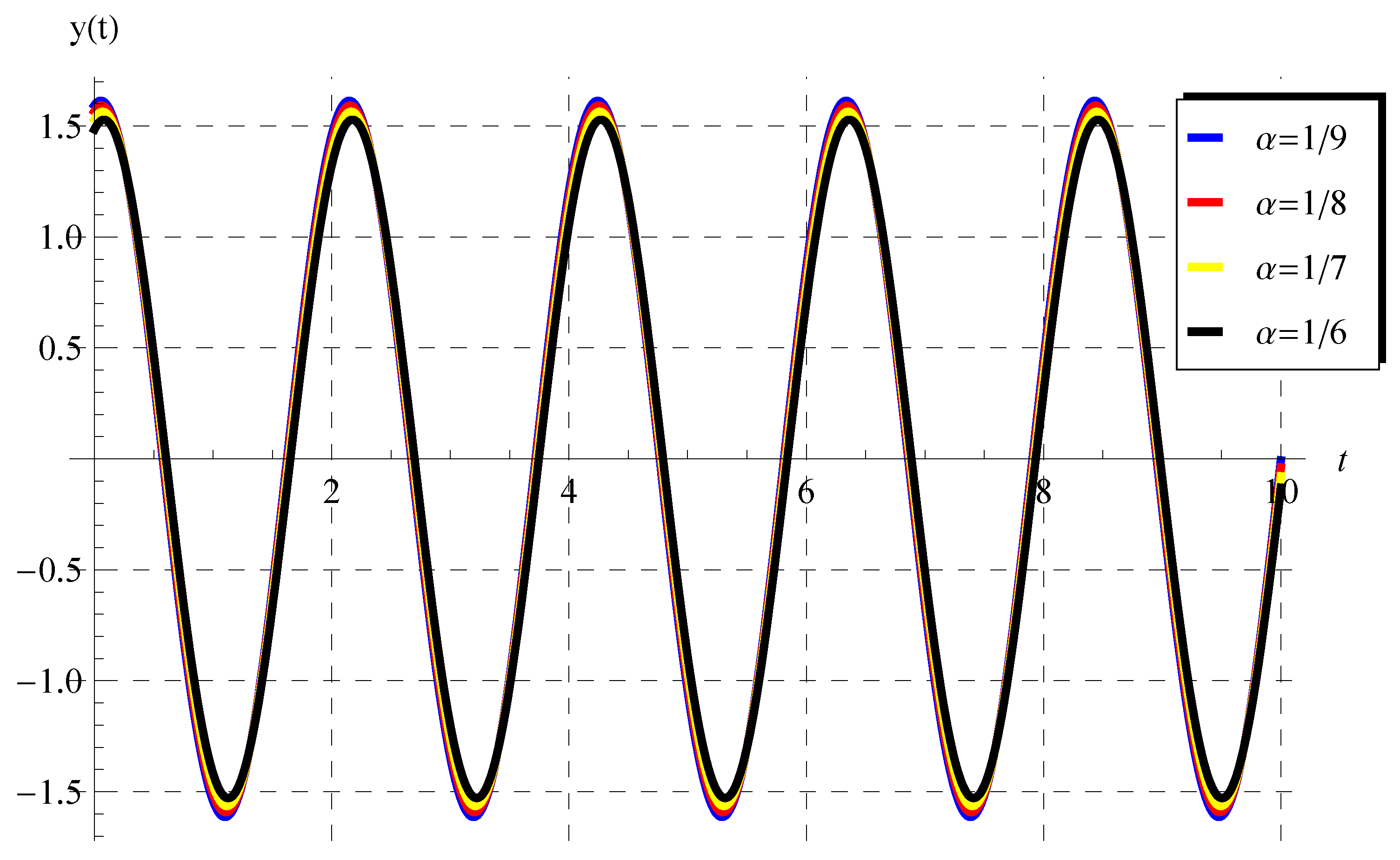
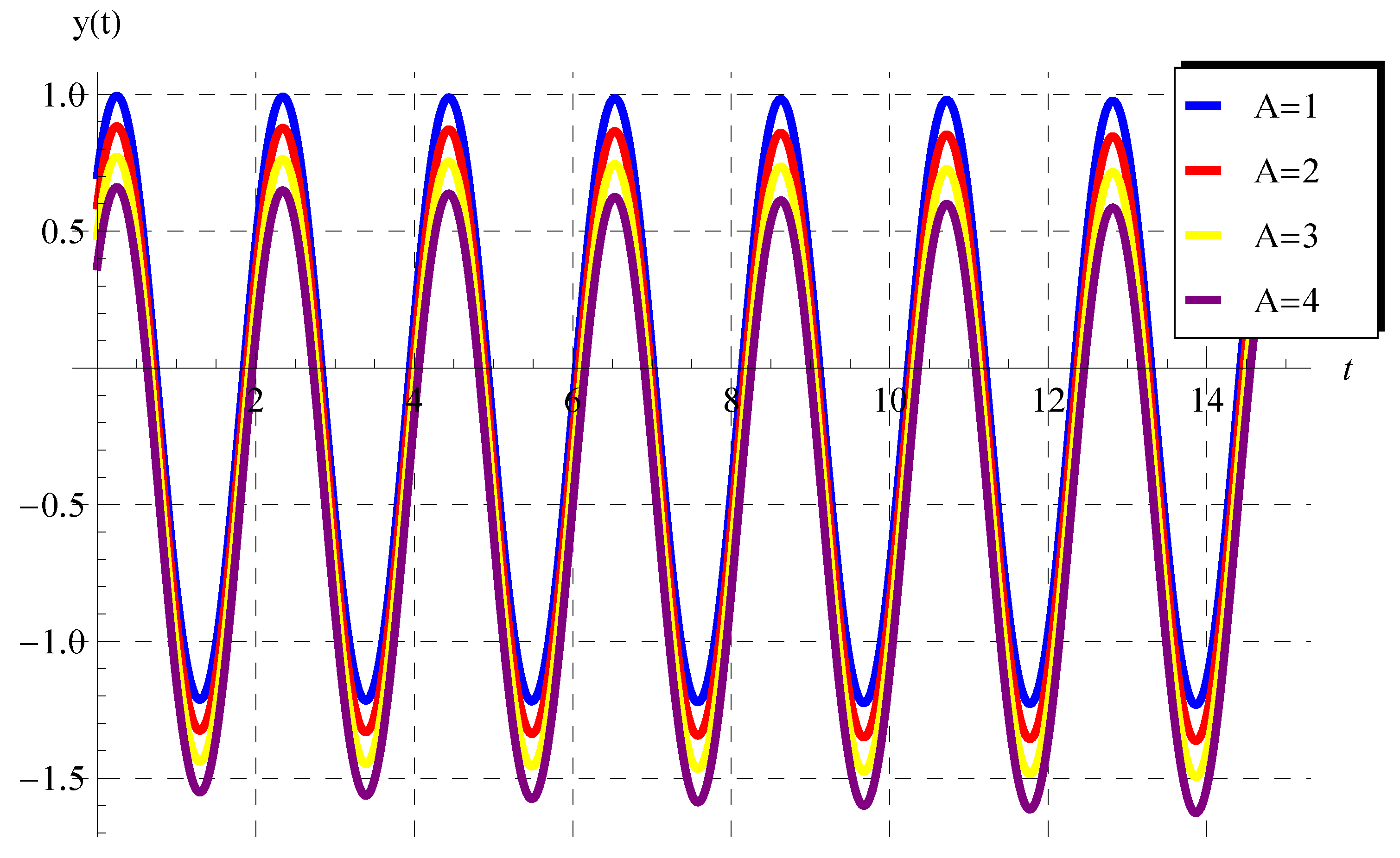
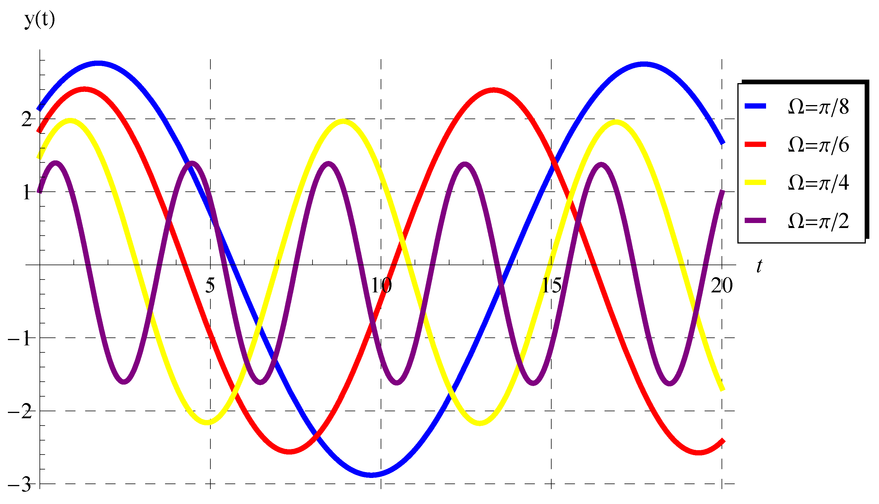
5. Characteristics of Solutions

For the class of 1st-order FIVP (1), it is observed that the exact solution in Equation (47) depends on whether the quantity ${\left(-{\omega }^2\right)}^{\frac{1}{\alpha }}$ is real or complex for $0<\alpha <1$. Since $\omega \in \mathbb{R}$, then the expression ${\left({\omega }^2\right)}^{\frac{1}{\alpha }}\in \mathbb{R}$ $\forall \alpha \in (0,1)$. If we write ${\left(-{\omega }^2\right)}^{\frac{1}{\alpha }}=ϵ{\left({\omega }^2\right)}^{\frac{1}{\alpha }}$, where $ϵ={(-1)}^{\frac{1}{\alpha }}$, then the solution is real/complex if $ϵ$ is real/complex. The following theorem determines the values of $\alpha$ for the real solutions of the 1st-order FIVP (1).

Theorem 2

(α-values for real solutions).The solution (47) is real at $\alpha =\frac{2n-1}{2(k+n-1)}$ ($ϵ=1$) and $\alpha =\frac{2n-1}{2(k+n)-1}$ ($ϵ=-1$), $\forall n,k\in {\mathbb{N}}^{+}$.

Proof. 

For $0<\alpha <1$, the fractional-order $\alpha$ can be assumed as $\alpha =\frac{l_1}{r_1}$ such that $0<l_1<r_1$. For odd $l_1$ and even $r_1$, the possible values of $\alpha$ belong to the sets $\{\frac{1}{2},\frac{1}{4},\frac{1}{6},\cdots \}$, $\{\frac{3}{4},\frac{3}{6},\frac{3}{8},\cdots \}$, $\{\frac{5}{6},\frac{5}{8},\frac{5}{10},\cdots \}$, $\{\frac{7}{8},\frac{7}{10},\frac{7}{12},\cdots \}$, ⋯, which can be written as ${\left\{\frac{1}{2k}\right\}}_{k=1}^{\infty }$, ${\left\{\frac{3}{2k+2}\right\}}_{k=1}^{\infty }$, ${\left\{\frac{5}{2k+4}\right\}}_{k=1}^{\infty }$, ⋯, and such sets can be unified as

$$\alpha =\frac{2n-1}{2(k+n-1)},\forall n,k\in {\mathbb{N}}^{+},$$

(49)

and in this case, we have $ϵ={(-1)}^{\frac{1}{\alpha }}={\left(-1\right)}^{\frac{2(k+n-1)}{2n-1}}=1$.

Furthermore, $\alpha$ can be assumed as $\alpha =\frac{l_1}{l_2}$ for two odd positive integers such that $0<l_1<l_2$. In this case, the values of $\alpha$ belong to the sets $\{\frac{1}{3},\frac{1}{5},\frac{1}{7},\cdots \}$, $\{\frac{3}{5},\frac{3}{7},\frac{3}{9},\cdots \}$, $\{\frac{5}{7},\frac{5}{9},\frac{5}{11},\cdots \}$, $\{\frac{7}{9},\frac{7}{11},\frac{7}{13},\cdots \}$, ⋯, which can be written as ${\left\{\frac{1}{2k+1}\right\}}_{k=1}^{\infty }$, ${\left\{\frac{3}{2k+3}\right\}}_{k=1}^{\infty }$, ${\left\{\frac{5}{2k+5}\right\}}_{k=1}^{\infty }$, ⋯, and such sets can be unified as

$$\alpha =\frac{2n-1}{2k+2n-1},\forall n,k\in {\mathbb{N}}^{+},$$

(50)

and we have $ϵ=-1$. Note that $ϵ\in \mathbb{C}$ if $\alpha =\frac{r_2}{l_2}$ for any even $r_2$ and any odd $l_2$ such that $0<r_2<l_2$. □

Numerical Results: Oscillatory Solution

In Figure 1, Figure 2, Figure 3 and Figure 4, the solution in Equation (47) is plotted at some selected values according to Theorem 2. The periodicity/oscillatory of the solution is clear in these figures. In addition, it can be seen from Figure 4 that our curves for those values of $\alpha$ near to 1 are identical to the ordinary case. Finally, Figure 5 and Figure 6 show the effect of the initial condition A and the parameter $\mathrm{\Omega }$ on the behavior of the solution.

6. Conclusions

A class of 1st-order FIVPs was investigated. This class is oscillatory in nature and hence of practical interest in engineering science. A dual solution was determined for the present class. The first solution was obtained through the LT and expressed in terms of the Mittag–Leffler functions. The second solution was derived via a newly developed approach in terms of exponential and trigonometric functions. The advantages of the second solution over the first one were demonstrated. In addition, it was revealed that the second solution is real at certain values of the fractional-order $\alpha$. Such values of $\alpha$ were derived theoretically. The behavior of the real solution was displayed through several figures. The present analysis may be introduced for the first time to obtain the solution with a straightforward approach. The developed approach can be extended to higher-order FIVPs of oscillatory types. Finally, such approach can be viewed as a corner stone to obtaining periodic solutions for more complex oscillatory problems, such as the forced Duffing oscillator [30].

References

1. Miller, K.S.; Ross, B. An Introduction to the Fractional Calculus and Fractional Differential Equations; John Wiley & Sons: New York, NY, USA, 1993. [Google Scholar]
2. Podlubny, I. Fractional Differential Equations; Academic Press: San Diego, CA, USA, 1999. [Google Scholar]
3. Hilfer, R. Applications of Fractional Calculus in Physics; World Scientific Publishing Company: Singapore, 2000. [Google Scholar]
4. Achar, B.N.N.; Hanneken, J.W.; Enck, T.; Clarke, T. Dynamics of the fractional oscillator. Physica A 2001, 297, 361–367. [Google Scholar] [CrossRef]
5. Sebaa, N.; Fellah, Z.E.A.; Lauriks, W.; Depollier, C. Application of fractional calculus to ultrasonic wave propagation in human cancellous bone. Signal Process. 2006, 86, 2668–2677. [Google Scholar] [CrossRef]
6. Tarasov, V.E. Fractional Heisenberg equation. Phys. Lett. A 2008, 372, 2984–2988. [Google Scholar] [CrossRef] [Green Version]
7. Ding, Y.; Yea, H. A fractional-order differential equation model of HIV infection of CD4+T-cells. Math. Comput. Model. 2009, 50, 386–392. [Google Scholar] [CrossRef]
8. Wang, S.; Xu, M.; Li, X. Green’s function of time fractional diffusion equation and its applications in fractional quantum mechanics. Nonlinear Anal. Real World Appl. 2009, 10, 1081–1086. [Google Scholar] [CrossRef]
9. Song, L.; Xu, S.; Yang, J. Dynamical models of happiness with fractional order. Commun. Nonlinear Sci. Numer. Simul. 2010, 15, 616–628. [Google Scholar] [CrossRef]
10. Gómez-Aguilara, J.F.; Rosales-García, J.J.; Bernal-Alvarado, J.J. Fractional mechanical oscillators. Rev. Mex. De Física 2012, 58, 348–352. [Google Scholar]
11. Machado, J.T.; Kiryakova, V.; Mainardi, F. Recent history of fractional calculus. Commun. Nonlinear Sci. Numer. Simul. 2011, 16, 1140–1153. [Google Scholar] [CrossRef] [Green Version]
12. Ebaid, A.; El-Sayed, D.M.M.; Aljoufi, M.D. Fractional calculus model for damped mathieu equation: Approximate analytical solution. Appl. Math. Sci. 2012, 6, 4075–4080. [Google Scholar]
13. Garcia, J.J.R.; Calderon, M.G.; Ortiz, J.M.; Baleanu, D. Motion of a particle in a resisting medium using fractional calculus approach. Proc. Rom. Acad. Ser. A 2013, 14, 42–47. [Google Scholar]
14. Machado, J.T. A fractional approach to the Fermi-Pasta-Ulam problem. Eur. Phys. J. Spec. Top. 2013, 222, 1795–1803. [Google Scholar] [CrossRef]
15. Ebaid, A. Analysis of projectile motion in view of the fractional calculus. Appl. Math. Model. 2011, 35, 1231–1239. [Google Scholar] [CrossRef]
16. Ebaid, A.; El-Zahar, E.R.; Aljohani, A.F.; Salah, B.; Krid, M.; Machado, J.T. Analysis of the two-dimensional fractional projectile motion in view of the experimental data. Nonlinear Dyn. 2019, 97, 1711–1720. [Google Scholar] [CrossRef]
17. Ahmad, B.; Batarfi, H.; Nieto, J.J.; Oscar, O.-Z.; Shammakh, W. Projectile motion via Riemann-Liouville calculus. Adv. Differ. Equ. 2015, 63, 1–14. [Google Scholar] [CrossRef] [Green Version]
18. Kumar, D.; Singh, J.; Baleanu, D.; Rathore, S. Analysis of a fractional model of the Ambartsumian equation. Eur. Phys. J. Plus 2018, 133, 133–259. [Google Scholar] [CrossRef]
19. Ebaid, A.; Cattani, C.; Juhani1, A.S.A.; El-Zahar, E.R. A novel exact solution for the fractional Ambartsumian equation. Adv. Differ. Equ. 2021, 2021, 88. [Google Scholar] [CrossRef]
20. El-Zahar, E.R.; Alotaibi, A.M.; Ebaid, A.; Aljohani, A.F.; Aguilar, J.F.G. The Riemann-Liouville fractional derivative for Ambartsumian equation. Results Phys. 2020, 19, 103551. [Google Scholar] [CrossRef]
21. Kaur, D.; Agarwal, P.; Rakshit, M.; Chand, M. Fractional Calculus involving (p, q)-Mathieu Type Series. Appl. Math. Nonlinear Sci. 2020, 5, 15–34. [Google Scholar] [CrossRef]
22. Agarwal, P.; Mondal, S.R.; Nisar, K.S. On fractional integration of generalized struve functions of first kind. Thai J. Math. 2020, in press. [Google Scholar]
23. Agarwal, P.; Singh, R. Modelling of transmission dynamics of Nipah virus (Niv): A fractional order approach. Phys. A Stat. Mech. Its Appl. 2020, 547, 124243. [Google Scholar] [CrossRef]
24. Alderremy, A.A.; Saad, K.M.; Agarwal, P.; Aly, S.; Jain, S. Certain new models of the multi space-fractional Gardner equation. Phys. A Stat. Mech. Its Appl. 2020, 545, 123806. [Google Scholar] [CrossRef]
25. Feng, Y.; Yang, X.; Liu, J.; Chen, Z. New perspective aimed at local fractional order memristor model on Cantor sets. Fractals 2020. accepted manuscript. [Google Scholar] [CrossRef]
26. Feng, Y.; Yang, X.; Liu, J. On overall behavior of Maxwell mechanical model by the combined Caputo fractional derivative. Chin. J. Phys. 2020, 66, 269–276. [Google Scholar] [CrossRef]
27. Sweilam, N.H.; Al-Mekhlafi, S.M.; Assiri, T.; Atangana, A. Optimal control for cancer treatment mathematical model using Atangana-Baleanu-Caputo fractional derivative. Adv. Differ. Equ. 2020, 334, 1–21. [Google Scholar] [CrossRef]
28. Atangana, A.; Qureshi, S. Mathematical Modeling of an Autonomous Nonlinear Dynamical System for Malaria Transmission Using Caputo Derivative. Fract. Order Anal. Theory Methods Appl. 2020, 9, 225–252. [Google Scholar] [CrossRef]
29. Elzahar, E.R.; Gaber, A.A.; Aljohani, A.F.; Machado, J.T.; Ebaid, A. Generalized Newtonian fractional model for the vertical motion of a particle. Appl. Math. Model. 2020, 88, 652–660. [Google Scholar] [CrossRef]
30. El-Dib, Y.O.; Elgazery, N.S. Effect of Fractional Derivative Properties on the Periodic Solution of the Nonlinear Oscillations. Fractals 2020, 28, 2050095. [Google Scholar] [CrossRef]
31. Ortigueira, M.D.; Machado, J.T.; Trujillo, J.J. Fractional derivatives and periodic functions. Int. J. Dynam. Control 2015, 5, 72–78. [Google Scholar] [CrossRef]
Figure 1. Plots of y ( t ) in Equation (47) vs. t when a = 2 , A = 1 , ω = 1 3 , and Ω = 3 at different values of α = 1 9 , 1 8 , 1 7 , 1 6 .
Fractalfract 06 00085 g001
Figure 2. Plots of y ( t ) in Equation (47) vs. t when a = 2 , A = 1 , ω = 1 3 , and Ω = 3 at different values of α = 1 4 , 1 2 , 3 4 , 7 8 .
Fractalfract 06 00085 g002
Figure 3. Plots of y ( t ) in Equation (47) vs. t when a = 2 , A = 1 , ω = 1 3 , and Ω = 3 at different values of α = 1 3 , 3 7 , 7 9 , 9 11 .
Fractalfract 06 00085 g003
Figure 4. Plots of y ( t ) in Equation (47) vs. t when a = 2 , A = 1 , ω = 1 3 , and Ω = 3 at different values of α = 27 29 , 45 47 , 61 63 , 81 83 , 1 .
Fractalfract 06 00085 g004
Figure 5. Plots of y ( t ) in Equation (47) vs. t when α = 1 2 , a = 2 , ω = 1 3 , and Ω = 3 at different values of A = 1 , 2 , 3 , 4 .
Fractalfract 06 00085 g005
Figure 6. Plots of y ( t ) in Equation (47) vs. t when α = 1 2 , A = 1 , a = 2 , and ω = 1 3 at different values of Ω = π / 8 , π / 6 , π / 4 , π / 2 .
Fractalfract 06 00085 g006
Publisher’s Note: MDPI stays neutral with regard to jurisdictional claims in published maps and institutional affiliations.