Article

Study on the Complex Dynamical Behavior of the Fractional-Order Hopfield Neural Network System and Its Implementation

1
School of Information Science and Engineering, Dalian Polytechnic University, Dalian 116034, China
2
Department of Mathematical Sciences, Giuseppe Luigi Lagrange, Politecnico di Torino, Corso Duca degli Abruzzi 24, I-10129 Torino, Italy
*
Authors to whom correspondence should be addressed.
Fractal Fract. 2022, 6(11), 637; https://doi.org/10.3390/fractalfract6110637
Submission received: 19 September 2022 / Revised: 26 October 2022 / Accepted: 26 October 2022 / Published: 1 November 2022

Abstract

:
The complex dynamics analysis of fractional-order neural networks is a cutting-edge topic in the field of neural network research. In this paper, a fractional-order Hopfield neural network (FOHNN) system is proposed, which contains four neurons. Using the Adomian decomposition method, the FOHNN system is solved. The dissipative characteristics of the system are discussed, as well as the equilibrium point is resolved. The characteristics of the dynamics through the phase diagram, the bifurcation diagram, the Lyapunov exponential spectrum, and the Lyapunov dimension of the system are investigated. The circuit of the system was also designed, based on the Multisim simulation platform, and the simulation of the circuit was realized. The simulation results show that the proposed FOHNN system exhibits many interesting phenomena, which provides more basis for the study of complex brain working patterns, and more references for the design, as well as the hardware implementation of the realized fractional-order neural network circuit.

1. Introduction

Dynamics studies of artificial neurons and neural networks are important for understanding brain functions and developing neuromorphic systems. In recent years, the modeling of memory neurons and neural networks has a great potential for brain dynamics studies [1,2,3,4]. The Hopfield neural network is a type of artificial neural network, abstracted from the human brain [5], which can generate complex dynamical behaviors, due to the active firing behavior of its internal neurons [6,7,8], and these behaviors include limit loops, chaotic states, stability, multi-stability coexistence, etc. Although the construction of this neural network is simple, it is better analyzed and studied to provide a better experimental basis for understanding the behavior and working mechanism of the brain [6,9,10,11].
In recent years, Hopfield’s neural network has increasingly attracted wide attention and research, as a typical model for studying the working mechanism and information storage of the brain [12,13,14,15]. For example, Li et al. [16] constructed a new dynamic neural network model consisting of three Hopfield neurons, revealing that the coupled weighted synapses of the memory can influence the distribution of the system’s equilibrium points. Ding et al. [17] found that the Hopfield Neural Network model of the coupled local activation memristors has a multiple stability at different fractional orders and coupling coefficients. Saeed Sani et al. proposed a new algorithm for the COVID-19 detection in chest CT images, based on the Hopfield neural network analysis [18]. It has made great contributions in solving associative memory and traveler problems, by using the Hopfield neural network [19,20,21,22]. These studies suggest that studying the complex dynamical behavior of the Hopfield neural network can provide more basis for the work related to brain dynamics, and it is necessary to study this neural network model in depth.
The fractional order calculus is a theory for studying the arbitrary order differentiation and integration [23], with a wide range of applications in memory digital image processing, engineering control, and other fields [24,25,26,27,28,29,30,31,32,33,34,35,36,37]. The weighted form of the fractional-order system allows for the accumulation of global information about the function and thus a greater memorability and freedom than the integer-order system, while the fractional-order calculus is closer to reality. The use of the fractional order allows to describe the physical objects, especially some physical phenomena, with memory, more accurately than the integer order and more in line with the biological neural networks applied to reality. Therefore, fractional order calculus has been introduced into artificial neural networks in some studies to construct more accurate mathematical models [38,39,40,41,42]. The research results show that fractional-order neural networks can more accurately model the activity of brain neurons than integer-order neural network systems. Therefore, fractional-order neural networks have great application prospects and research value.
However, in the present research results, more integer-order neural network models are discussed. In the process of model building, the influence of the fractional order on the model is neglected, especially in the process of building some circuit models, the fractional order impedance that plays a decisive role in the actual electronic devices, is not taken into account. The implementation of the fractional-order neural network systems is also relatively rare in the existing studies [43,44,45]. Based on this, the fractional order theory is introduced into the Hopfield neural network system to construct a new class of the FOHNN system.
The main work of this paper is to construct a fractional-order Hopfield neural network (FOHNN) system, using the Adomian solution method algorithm, to explore the rich and complex dynamical properties present in the system, and to design a circuit for the FOHNN system. The rest of the components are as follows: Section 2 presents the FOHNN system, based on four neurons and the ADM decomposition of the system. In Section 3, some dynamical behaviors of the proposed model are analyzed. The circuit of the system is designed in Section 4 and based on the Multisim platform, the simulation is verified. In Section 4, a 4D FOHNN system is implemented, based on Multisim. In the end, some conclusions were drawn.

2. FOHNN System with Four Neurons

2.1. Principle of the Fractional Calculus

Currently, there are various definitions of the fractional order calculus, and the most commonly used ones are the Grunwald–Letnikov (G–L) derivative, the Riemann–Liouville (R–L) derivative and the Caputo derivative. These three definitions are not equivalent. However, the physical meaning of the Caputo differential definition is very clear, since only the value of the initial condition needs to be determined, when it is adopted. The Caputo definition is more conducive to the actual physical system solution and has a more practical engineering application.
Definition 1 
[46]. The Caputo fractional differentiation is defined as
D t q f ( t ) = J t 0 m q D t 0 m f ( t ) = { 1 Γ ( m q ) 0 t f ( m ) ( τ ) d τ ( t τ ) q + 1 m , m 1 < q < m d m d t m f ( t ) , q = m ,
where q R+, m N, D t q is the q-order Caputo differential operator. Γ represents the Gamma function.
Definition 2 
[47]. The Laplace transform of the fractional order differentiation is
L [ 0 D t 0 q f ( t ) ] = 0 e s t D t 0 q f ( t ) d t = s q F ( s ) k = 0 m 1 s k [ D t 0 q k 1 f ( t ) ] | t = 0 , m 1 < q < m ,
where F(s) = L [f(t)] denotes the Laplace transform of f(t).
Theorem 1 
[48]. The linear autonomous system
D c q x = A x ,
where A R n × n and q (0,1) is asymptotically stable if and only if
| arg ( λ ) | > q π 2 , λ σ ( A ) ,
or, if and only if
| Re ( λ ) | > Im ( λ ) q π 2 , λ σ ( A ) ,
where σ ( A ) represents the set of all eigenvalues of the matrix A.
The proposed fractional order differential equation D t 0 q v(t) = f(v(t)), based on the Adomian solution method (ADM), can be expressed in the form,
D t 0 q v ( t ) = L v ( t ) + N v ( t ) + C ( t )
where * D t 0 q stands for the Caputo derivative operator of the order q (m−1 < qm, mN), v(t) = [v1(t) v2(t) … vn(t)] T are the state variables. The linear and nonlinear terms are denoted by L and N, respectively. C(t) = [C1(t) C2(t) … Cn(t)] T is the constant for the autonomous system. By applying the J t 0 q to the left and right of Equation (1), the following equation can be obtained
x ( t ) = J t 0 q L v ( t ) + J t 0 q N v ( t ) + J t 0 q C + v ( t t 0 + ) ,
where J t 0 q indicates the R-L fractional integral operator of order q, the initial value is given by v( t t 0 + ). According to ADM description, it can be known that the operational property of the integral operator J t 0 q , are shown as follows:
J t 0 q C = C Γ ( q + 1 ) ( t t 0 ) q ,
J t 0 q ( t t 0 ) γ = Γ ( γ + 1 ) Γ ( γ + 1 + q ) ( t t 0 ) q + γ ,
J t 0 q J t 0 r v ( t ) = J t 0 q + r v ( t ) ,
where t ∈ [t0, t1], q ≥ 0, γ > −1, r ≥ 0. The i-th nonlinear term can be solved using the following
{ A j i = 1 i ! [ d i d λ i N ( v j i ( λ ) ) ] λ = 0 v j i ( λ ) = k = 1 i ( λ ) k v j k ,
in which i = 0, 1, 2, 3 … ∞; j = 1, 2, 3… n. The nonlinear term N is recorded as
N v = i = 0 A i ( v 0 , v 1 , , v i ) ,
Therefore, using the following form to represent the numerical solution of the system (1)
v = i = 1 v i = J t 0 q i = 1 v i + J t 0 q i = 1 A i + J t 0 q C + v ( t 0 + ) ,
where vi is calculated by
v 0 = J t 0 q C + v ( t 0 ) , v 1 = J t 0 q L v 0 + J t 0 q A 0 ( v 0 ) , v 2 = J t 0 q L v 1 + J t 0 q A 1 ( v 0 , v 1 ) , v n = J t 0 q L v i 1 + J t 0 q A i 1 ( v 0 , v 1 , v i 1 ) . ,

2.2. Solution of the FOHNN-Based System

In 1982, J. Hopfield proposed the Hopfield neural network model
C i d v i d t = v i R i + j = 1 n T i j g j ( v j ) + I i , i = 1 , 2 , , n ,
where Ri, Ci, and Ti represents the resistance, capacitance, and conductance, respectively, and gi(vi) is the activation function generated by the operational amplifier. Normally, the selection of an as one, and when the hyperbolic tangent function is chosen as the activation function, the chaotic attractors appear in the system. The weight matrix Tij is modified and its dimension is determined by the number of neurons. In this FOHNN system, Tij has size 4 × 4, meaning that the Hopfield neural network has four state variables, associated with each neuron. The topology structure of the neural network is shown in Figure 1.
[ v ˙ 1 v ˙ 2 v ˙ 3 v ˙ 4 ] = [ v 1 v 2 v 3 v 4 ] + T [ g ( v 1 ) g ( v 2 ) g ( v 3 ) g ( v 4 ) ] , [ g ( v 1 ) g ( v 2 ) g ( v 3 ) g ( v 4 ) ] = [ tanh ( v 1 ) tanh ( v 2 ) tanh ( v 3 ) tanh ( v 4 ) ] , T i j = [ T 11 T 12 T 13 T 14 T 21 T 22 T 23 T 24 T 31 T 32 T 33 T 34 T 41 T 42 T 43 T 44 ] .
Setting Ri = 1, Ii = 0, the Equation (16) describes the model, based on four neurons. In this case, the v is a vector containing the four elements with the four state variables. Two variable synaptic weighting parameters are set, namely β1 and β2. By choosing the corresponding synaptic weight coefficients, the synaptic weight matrix is represented as follows
T = [ 0.3 0.5 0 0.1 2.3 β 1 8.5 0 4 0 0 1 35 β 2 0 1 ]
According to Definitions 1 and 2, a fractional order form of a fourth-FOHNN system can be written as
{ D t 0 q v 1 ( t ) = v 1 + 0.3 tanh ( v 1 ) + 0.5 tanh ( v 2 ) + 0.1 tanh ( v 4 ) D t 0 q v 2 ( t ) = v 2 + 2.3 tanh ( v 1 ) + β 1 tanh ( v 2 ) + 8.5 tanh ( v 3 ) D t 0 q v 3 ( t ) = v 3 4 tanh ( v 1 ) + tanh ( v 4 ) D t 0 q v 4 ( t ) = v 4 + 35 tanh ( v 1 ) + β 2 tanh ( v 2 ) + tanh ( v 4 ) ,
where q represents the order of the FOHNN system. Based on the ADM algorithm, the linear and nonlinear terms of the system are represented as
[ L v 1 L v 2 L v 3 L v 4 ] = [ v 1 v 2 v 3 v 4 ] , [ N v 1 N v 2 N v 3 N v 4 ] = [ tanh ( v 1 ) tanh ( v 2 ) tanh ( v 3 ) tanh ( v 4 ) ] , [ c 1 c 2 c 3 c 4 ] = [ 0 0 0 0 ] ,
For the consideration of the convergence speed of the ADM algorithm, the first five terms are intercepted here under the premise of guaranteeing the accuracy. According to Equation (6), the decomposition of A1 = tanh(v1) as an example, can be decomposed as follows
A 1 0 = tanh ( v 1 0 ) A 1 1 = v 1 1 sech 2 ( v 1 0 ) A 1 2 = v 1 2 sech 2 ( v 1 0 ) ( v 1 1 ) 2 sech 2 ( v 1 0 ) tanh ( v 1 0 ) A 1 3 = v 1 3 sech 2 ( v 1 0 ) 2 v 1 2 v 1 1 sech 2 ( v 1 0 ) tanh ( v 1 0 ) + 1 3 ( v 1 1 ) 3 ( 4 sech 3 ( v 1 0 ) tanh 2 ( v 1 0 ) sech 4 ( v 1 0 ) ) A 1 4 = x 1 4 sech 2 ( v 1 0 ) ( 2 v 1 3 v 1 1 + v 1 2 v 1 2 ) sech 2 ( v 1 0 ) tanh ( v 1 0 ) + v 1 1 v 1 1 v 1 2 ( 4 sech 3 ( v 1 0 ) tanh 2 ( v 1 0 ) sech 4 ( v 1 0 ) ) + 1 3 ( v 1 1 ) 4 ( sech 3 ( v 1 0 ) tanh ( v 1 0 ) 3 sech 3 ( v 1 0 ) tanh 3 ( v 1 0 ) )
The other three nonlinear terms are similar to A1. Setting the initial value v0 = [v1( t 0 + ) v2( t 0 + ) v3( t 0 + ) v4( t 0 + )]t, the first term can be gained for
{ v 1 0 = v 1 ( t 0 + ) v 2 0 = v 2 ( t 0 + ) v 3 0 = v 3 ( t 0 + ) v 4 0 = v 4 ( t 0 + )
Letting c 1 0 = v 1 0 , c 2 0 = v 2 0 , c 3 0 = v 3 0 , c 4 0 = v 4 0 therefore we obtain v0 = c0= [ c 1 0   c 2 0   c 3 0   c 4 0 ]. v1= J t 0 q Lv0 + J t 0 q A0(v0) is obtained by the iterative relation formula Equation (14). The second term of the state variables are expressed as
{ x 1 1 = ( c 1 0 + 0.3 tanh ( c 1 0 ) + 0.5 tanh ( c 2 0 ) + 0.1 tanh ( c 4 0 ) ) ( t t 0 ) q Γ ( q + 1 ) x 2 1 = ( c 2 0 + 2.3 tanh ( c 1 0 ) + β 1 tanh ( c 2 0 ) + 8.5 tanh ( c 3 0 ) ) ( t t 0 ) q Γ ( q + 1 ) x 3 1 = ( c 3 0 4 tanh ( c 1 0 ) + tanh ( c 4 0 ) ) ( t t 0 ) q Γ ( q + 1 ) x 4 1 = ( c 4 0 + 35 tanh ( c 1 0 ) + β 2 tanh ( c 2 0 ) + tanh ( c 4 0 ) ) ( t t 0 ) q Γ ( q + 1 ) .
Let
{ c 1 1 = c 1 0 + 0.3 tanh ( c 1 0 ) + 0.5 tanh ( c 2 0 ) + 0.1 tanh ( c 4 0 ) c 2 1 = c 2 0 + 2.3 tanh ( c 1 0 ) + β 1 tanh ( c 2 0 ) + 8.5 tanh ( c 3 0 ) c 3 1 = c 3 0 4 tanh ( c 1 0 ) + tanh ( c 4 0 ) c 4 1 = c 4 0 + 35 tanh ( c 1 0 ) + β 2 tanh ( c 2 0 ) + tanh ( c 4 0 ) ,
So v1 will be represented as x1 = c1(tt0)q/Γ(q + 1). By using the same method, the coefficient decompositions of the other four terms are listed in Appendix A.
Therefore, the numerical results of the five-term system, based on FOHNN are
x ˜ j = c j 0 + c j 1 ( t t 0 ) q Γ ( q + 1 ) + c j 2 ( t t 0 ) 2 q Γ ( 2 q + 1 ) + c j 3 ( t t 0 ) 3 q Γ ( 3 q + 1 ) + c j 4 ( t t 0 ) 4 q Γ ( 4 q + 1 ) + c j 5 ( t t 0 ) 5 q Γ ( 5 q + 1 )
here j = 1, 2, 3, 4, 5. In the process of the calculation, the whole interval is divided into many subintervals, and the value obtained from the previous subinterval will be used as the initial value of the latter subinterval for iteration, with an iteration step of h. Setting β1 = 0.72, β2 = 12.5, q = 0.55, h = 0.01, and initial values x0= (0.2, 0.2, 0.1, 0.5). The FOHNN-based system’s Lyapunov exponents are L1 = 1.7610, L2 = 0, L3 = −6.8754, and L4 = −6.8754 and the Lyapunov dimension is DL = 2.2561. With a positive maximum Lyapunov exponent, the system has a chaotic attractor. The phase diagram of the chaotic attractor, based on the FOHNN system are displayed in Figure 2.

3. Study of the Dynamical Characteristics of the FOHNN System

3.1. Dissipation of the FOHNN System with the Existence of Attractors

The dispersion of an alternative nonlinear system to be in a chaotic state. For Equation (13), the dispersion of the FOHNN system is expressed as
V = div V = v ˙ 1 v 1 + v ˙ 2 v 2 + v ˙ 3 v 3 + v ˙ 4 v 4
according to Equations (13) and (24), the obtained
V = 4 0.3 sec h 2 ( v 1 ) + β 1 sec h 2 ( v 2 ) + sec h 2 ( v 4 )
due to 0 ≤ sech2(v1) ≤ 1, 0 ≤ sech2(v2) ≤ 1, 0 ≤ sech2(v4) ≤ 1, therefore, ≤ −4 − 0.3 + β1 + 1 < 0. Obviously, β1 < 3.3, the chaotic attractors will emerge from the system.

3.2. Stability Analysis of the Equilibrium Point of the FOHNN System

In order to obtain the equilibrium points, set the left of the equal sign of Equation (13) be 0 and solve the equation to obtain all of the equilibrium points of the system
{ v 1 0.3 tanh ( v 1 ) + 0.5 tanh ( v 2 ) + tanh ( v 4 ) = 0 v 2 + 2.3 tanh ( v 1 ) + β 1 tanh ( v 2 ) + 8.5 tanh ( v 3 ) = 0 v 3 4 tanh ( v 1 ) + tanh ( v 4 ) = 0 v 4 + 35 tanh ( v 1 ) + β 2 tanh ( v 2 ) + tanh ( v 4 ) = 0
It is obvious that Equation (27) is a system of the fourth order transcendental equations and all solutions of the equations need to be obtained using MATLAB. The Jacobian matrix of the system in any equilibrium point is
J = [ 0.3   sech 2 ( v 1 ) 1 0.5   sech 2 ( v 2 ) 0 sech 2 ( v 4 ) 2.3   sech 2 ( v 1 ) β 1 sech 2 ( v 2 ) 1 8.5   sech 2 ( v 3 ) 0 4   sech 2 ( v 1 ) 0 1 sech 2 ( v 4 ) 35   sech 2 ( v 1 ) β 2 sech 2 ( v 2 ) 0 sech 2 ( v 4 ) 1 ]
where sech2(i) = (1 − tanh2(i)) with I = v1, v2, v3, v4. Observing Equation (27), the system always exists a zero equilibrium point E0 = (0, 0, 0, 0), whatever the value of the parameter is taken. Setting β1 = 0.2, β2 = 15 the characteristic function of the equilibrium as
λ 4 + 2.5 λ 3 34.09 λ 2 + 81.41 λ + 457 = 0
the corresponding eigenvalues are −2.8701 ± 1.1582i and 2.8701 ± 2.3224i, and the |larg(λ2)| = 0.3835. According to Theorem 1, the equilibrium point is unstable and the system generates chaotic attractors, due to the existence of two conjugate complex roots with real parts greater than zero.

3.3. Stability Analysis of the Equilibrium Point of the FOHNN System

3.3.1. The Influence of the Different Orders of the FOHNN System

In order to study the influences of the different orders of the FOHNN system, the bifurcation diagram, the Lyapunov exponential spectrum, and the Lyapunov dimension of the system, were plotted in the variation of the q values from 0.2 to 1, as shown in Figure 3a–c. Setting h = 0.01, β1 = 0.4, and β2 = 12, the initial point v0 = (0.2, 0.1, 0.3, 0.2). It is emphasized that in order to eliminate the effect of the transition states, the excessive number of points generated in the calculation process, is appropriately rounded off. From Figure 4a, the FOHNN system is in a periodic state when 0.3 < q < 0.426. 0.426 < q < 1, the HNN-based fractional order system appears the chaotic attractors. At q ∈ (0.426, 1), there are multiple periodic windows of the system, which are shown in Table 1. Figure 3b–c is in perfect agreement with Figure 3a. The Lyapunov exponent of the system is positive and its Lyapunov dimension is greater than 2, which implies that the system has the chaotic attractors. Different types of attractors of the FOHNN system at different orders are plotted in Figure 4.

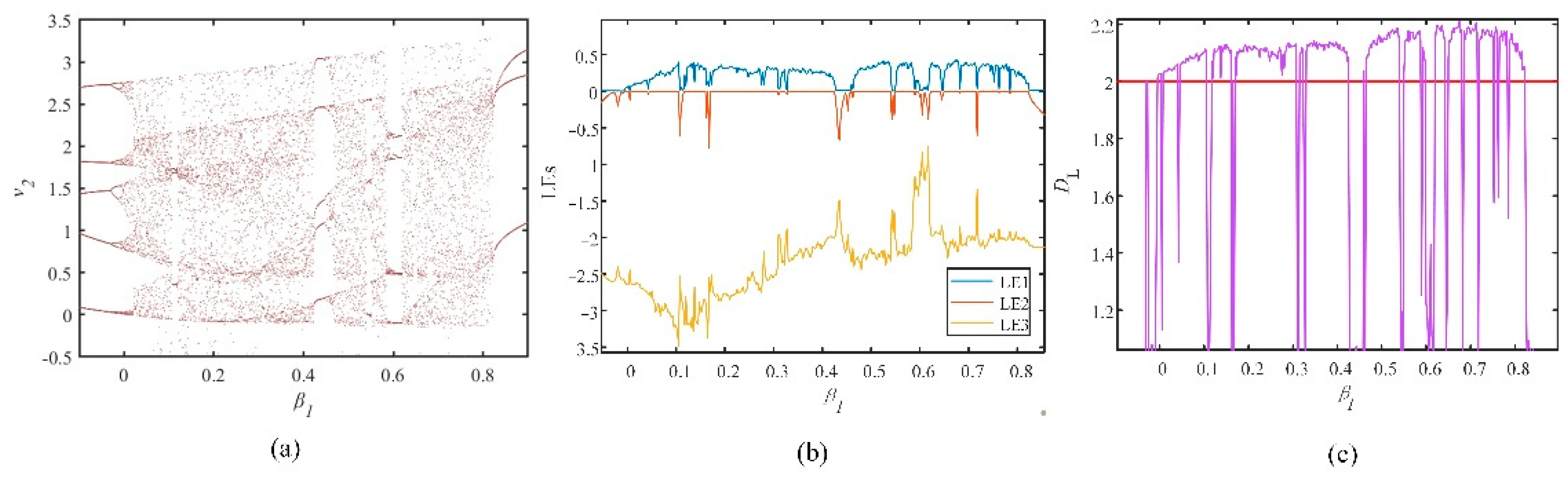
3.3.2. The Influence of the Different Synaptic Weights of the FOHNN System

Changing the different synaptic weight values, FOHNN presents rich and complex characteristics of the dynamics. Consider the influence of the alterations in two synaptic weights, β1 and β2, on the FOHNN system. When the fixed parameters β2 = 12, q = 0.8, h = 0.01, and β1∈ (0, 0.8), the bifurcation diagram of the system, Lyapunov exponents spectrum, Lyapunov dimension diagram are drawn in Figure 5a–c. When β1 < 0, the FOHNN system is in the periodic state; β1 > 0, chaotic attractors are generated and return to the periodic state again after a few periodic windows with β1 > 0.8. To better illustrate the state of the attractor, the attractor phase diagrams are presented in Figure 6 for the different β2.
When fixing the parameters β1 = 0.2, q = 0.8, h = 0.01, and β2 ∈ (6, 20), the FOHNN system appears to have more complex characteristics of the dynamics. Furthermore, the Lyapunov exponential spectrum of the system, the bifurcation diagram, Lyapunov dimension diagram, are presented and plotted in Figure 7. The phase diagrams of the different types of attractors are drawn in Figure 8. When β2 ∈ (6, 8.65), the system generates the period-2 attractor through the period-doubling bifurcation and produces the period attractor again after a short chaotic state. It enters the chaotic state again through the period-doubling bifurcation, and later produces the chaotic attractors after the period window. Compared with the integer-order HNN system, the FOHNN system appears to have more complex dynamics characteristics.

3.4. Coexistence of the Attractors with the Different Synaptic Weights

During the dynamical analysis, the multiple attractor coexistence phenomena were observed in the FOHNN system. Setting h = 0.01 and β1 = 0.5, β2 = 12, the coexistence of the attractors can be observed for the different initial values selected, including the coexistence of the limit loops with the limit loops and the coexistence of the chaotic attractors. The initial values v0 = (1, 0.1, 0.1, −0.1) and v1 = (−1, 0, 0.1, 0.1) are chosen to observe the coexistence of the attractors through the v3v4 phase plane. In Figure 9, with the increase of order q, the limit loops of coexistence are moving closer and closer, and when q = 0.9, the double scroll-double coexistence appears. Setting q = 0.5, β1 = 0.5, and changing the value of β2, we observe the attractor coexistence through the v1v4 phase plane in Figure 10. With the increase of the synaptic weight β2, the attractors gradually intermingle together. The complex attractor coexistence phenomenon further indicates that this FOHNN system has rich dynamical properties.

3.5. Transient Chaos in the FOHNN System

The emergence of chaos with a finite lifetime, is called the transient chaos. Usually, in a system, an appropriate region is selected in which the system moves in an apparently chaotic behavior and suddenly, at some point, the system immediately reaches a steady state, which can be a periodic behavior or a point of equilibrium. If it turns to chaotic motions, but they are different from the previous chaotic state, it is called a state transition. Transient chaos appears even in very common everyday life: transient chaos can occur in any system that moves irregularly, for a period of time, and then changes to a regular behavior. Based on this, the FOHNN system was studied in relation to this system, in which the transient chaos was found.
By choosing the parameters q = 0.8, β1 = 0.5, k = 14, and the initial value v0 = (0.1, 0.1, −0.2, 0.1), In order to observe the phenomenon conveniently, the horizontal axis of the coordinates is set to time t, and 100 points are set to 1 s. Through the relevant experiments, it can be clearly observed that when t = 1500 s, (N = 150,000), a funny phenomenon appears in the system. The transition from the chaotic state to the periodic state. Figure 11a presents a chaotic sequence diagram of the process, where the FOHNN system is in a chaotic state at 0 s < t < 700 s, and the system generates the periodic attractors at 700 s < t < 1500 s. For a better illustration of the change of state, the Lyapunov exponents and time evolution branch diagram are plotted, as shown in Figure 11b,c. The Lyapunov exponent spectrum fits well with the bifurcation diagram. The maximum Lyapunov exponent L1 = 0.327 at t = 100 s, and the value of LEs reaches 0 at t = 700 s as the time proceeds. In Figure 12, the phase diagrams of the periodic and chaotic attractors, when the FOHNN is at different times, and their time series are drawn. It is shown that the proposed FOHNN system has rich dynamical properties and better chaotic characteristics, and it is more appropriate for the study of the neural network dynamics.

4. Circuit Design and Simulation of the FOHNN System

To better demonstrate the realizability of the theoretical and mathematical model of the FOHNN system, the circuit of the FOHNN system is designed, based on the relevant devices of the analog circuit, as shown in Figure 13. The Tanh and F modules in the design diagram represent the tanh unit circuit and the fractional order unit circuit, and their detailed design can be shown in Figure 14. The design of the fractional order unit circuit is based on its mathematical expression, which can be described as
F ( s ) = R 1 s R 1 C 1 + 1 + R 2 s R 2 C 2 + 1 + R 3 s R 3 C 3 + 1 + + R n s R n C n + 1
Based on this, the designed FO unit circuit is as shown in Figure 14b.
Setting β1 = 0.35, β2 = 19, q1 = q2 = q3 = q = 0.95, and the initial value of the FOHNN system v0= (0.2, 0.1, 0.3, 0.2), the differential equation of the FOHNN system, based on Kirchhoff’s law and the circuit design, can be expressed as
{ D t q V 1 = ( 1 R 5 V 1 + R 3 R 2 R 4 tanh ( V 1 ) + R 15 R 14 R 6 tanh ( V 2 ) + R 38 R 37 R 9 tanh ( V 4 ) ) R 12 R 8 R 11 D t q V 2 = ( 1 R 17 V 2 + R 3 R 2 R 16 tanh ( V 1 ) + R 15 R 14 R 6 tanh ( V 2 ) + R 38 R 37 R 9 tanh ( V 3 ) ) R 23 R 19 R 22 D t q V 3 = ( 1 R 29 V 3 1 R 27 tanh ( V 1 ) + R 38 R 37 R 31 tanh ( V 4 ) ) R 32 R 35 R 34 D t q V 4 = ( 1 R 29 V 4 + R 3 R 2 R 39 tanh ( V 1 ) + R 15 R 14 R 40 tanh ( V 2 ) + R 38 R 37 R 41 tanh ( V 4 ) ) R 46 R 43 R 45
According to the system equations and the designed circuit, setting the corresponding values is listed in Table 2.
The relevant parameters are set and the circuit is connected, the output of Multisim simulation of the proposed FOHNN system is shown in Figure 15, which better verifies the implement ability of the FOHNN system.
A Monte Carlo analysis of the circuit was performed for a 5% tolerance of each component value, in the fractional-order cell circuit, based on a Gaussian distribution. Since the FOHNN system is of equal order, only one unitary circuit is analyzed here, as an example. Following the 2000 experiments in the Multisim environment, Figure 16 shows the transient analysis output of the Monte Carlo circuit, with a voltage average of 0.01502 V and an output voltage standard deviation of 0.0023 V. The circuit performs the fractional order function.

5. Conclusions

In this paper, a new class of a fractional-order neural network system is designed, based on the Hopfield neural network, solved by the ADM algorithm. The dissipative and bound properties of the system are drawn. The effects of the order q and the changes of the two synaptic weights β1 and β2 in the system, on the dynamic characteristics of the system, were analyzed, and the results showed that the system exhibited complex dynamical behaviors with the dynamic changes of the three parameters. Interestingly, the attractor coexistence phenomenon, as well as the transient chaos phenomenon, are also found. The circuit of the system was designed and experimentally verified using the Multisim simulation platform, and the experimental results verified the correctness of the theory and provided the possibility for the application of the neural network system in the actual applications. Therefore, the complex nonlinear phenomena and rich dynamical behaviors, exhibited by the FOHNN system, provide more experimental evidence for the system in the study of the neural network dynamics and the practical applications of fractional-order systems. The next step will be to consider the implementation of the actual circuit of the system and the application of the system to the image encryption, based on the chaotic sequences, etc., to provide more reference for further research.

Author Contributions

Data curation, H.Y.; Funding acquisition, B.L.; Project administration, J.M. and S.B.; Writing–original draft, T.M. All authors have read and agreed to the published version of the manuscript.

Funding

This work was supported by the National Natural Science Foundation of China (Grant Nos. 62061014); The Natural Science Foundation of Liaoning province (2020-MS-274); The Basic Scientific Research Projects of Colleges and Universities of Liaoning Province (Grant Nos. LJKZ0545).

Institutional Review Board Statement

Not applicable.

Informed Consent Statement

Not applicable.

Data Availability Statement

Not applicable.

Acknowledgments

The authors thank the referees for their detailed reading and comments that were both helpful and insightful.

Conflicts of Interest

The authors declare no conflict of interest.

Appendix A

{ c 1 2 = c 1 1 + 0.3 c 1 1 sech 2 ( c 1 0 ) + 0.5 c 2 1 sech 2 ( c 2 0 ) + 0.1 c 4 1 sech 2 ( c 4 0 ) c 2 2 = c 2 1 + 2.3 c 1 1 sech 2 ( c 1 0 ) + β 1 c 2 1 sech 2 ( c 2 0 ) + 8.5 c 3 1 sech 2 ( c 3 0 ) c 3 2 = c 3 1 4 c 1 1 sech 2 ( c 1 0 ) + c 4 1 sech 2 ( c 4 0 ) c 4 2 = c 4 1 + 35 c 1 1 sech 2 ( c 1 0 ) + β 2 c 2 1 sech 2 ( c 2 0 ) + c 4 1 sech 2 ( c 4 0 ) ,
{ c 1 3 = c 1 2 + 0.3 c 1 2 sech 2 ( c 1 0 ) + 0.5 c 2 2 sech 2 ( c 2 0 ) + 0.1 c 4 2 sech 2 ( c 4 0 ) + ( ( 0.3 c 1 1 c 1 1 sech 2 ( c 1 0 ) tanh ( c 1 0 ) 0.5 c 2 1 c 2 1 sech 2 ( c 2 0 ) tanh ( c 2 0 ) 0.1 c 4 1 c 4 1 sech 2 ( c 4 0 ) tanh ( c 4 0 ) ) Γ ( 2 q + 1 ) Γ 2 ( q + 1 ) ) c 2 3 = c 2 2 + 2.3 c 1 2 sech 2 ( c 1 0 ) + β 1 c 2 2 sech 2 ( c 2 0 ) + 8.5 c 3 2 sech 2 ( c 3 0 ) + ( ( 2.3 c 1 1 c 1 1 sech 2 ( c 1 0 ) tanh ( c 1 0 ) β 1 c 2 1 c 2 1 sech 2 ( c 2 0 ) tanh ( c 2 0 ) 8.5 c 3 1 c 3 1 sech 2 ( c 3 0 ) tanh ( c 3 0 ) ) Γ ( 2 q + 1 ) Γ 2 ( q + 1 ) ) c 3 3 = c 3 2 4 c 1 2 sech 2 ( c 1 0 ) + c 4 2 sech 2 ( c 4 0 ) + ( ( c 1 1 c 1 1 sech 2 ( c 1 0 ) tanh ( c 1 0 ) c 4 1 c 4 1 sech 2 ( c 4 0 ) tanh ( c 4 0 ) ) Γ ( 2 q + 1 ) Γ 2 ( q + 1 ) ) c 4 3 = c 4 2 + 35 c 1 2 sech 2 ( c 1 0 ) + β 2 c 2 2 sech 2 ( c 2 0 ) + c 4 2 sech 2 ( c 4 0 ) + ( ( 35 c 1 1 c 1 1 sech 2 ( c 1 0 ) tanh ( c 1 0 ) β 2 c 2 1 c 2 1 sech 2 ( c 2 0 ) tanh ( c 2 0 ) c 4 1 c 4 1 sech 2 ( c 4 0 ) tanh ( c 4 0 ) ) Γ ( 2 q + 1 ) Γ 2 ( q + 1 ) )
{ c 1 4 = c 1 3 + 0.3 c 1 3 sech 2 ( c 1 0 ) + 0.5 c 2 3 sech 2 ( c 2 0 ) + 0.1 c 4 3 sech 2 ( c 4 0 ) + ( ( 0.6 c 1 2 c 1 1 sech 2 ( c 1 0 ) tanh ( c 1 0 ) c 2 2 c 2 1 sech 2 ( c 2 0 ) tanh ( c 2 0 ) 0.2 c 4 2 c 4 1 sech 2 ( c 4 0 ) tanh ( c 4 0 ) ) Γ ( 3 q + 1 ) Γ ( q + 1 ) Γ ( 2 q + 1 ) ) + 0.1 ( c 1 1 ) 3 ( 4 sech 3 ( c 1 0 ) tanh 2 ( c 1 0 ) sech 4 ( c 1 0 ) ) + 1 6 ( c 2 1 ) 3 ( 4 sech 3 ( c 2 0 ) tanh 2 ( c 2 0 ) sech 4 ( c 2 0 ) ) + 1 30 ( c 4 1 ) 3 ( 4 sech 3 ( c 4 0 ) tanh 2 ( c 4 0 ) sech 4 ( c 4 0 ) ) Γ ( 3 q + 1 ) Γ 3 ( q + 1 ) ) c 2 4 = c 2 3 + 2.3 c 1 3 sech 2 ( c 1 0 ) + β 1 c 2 3 sech 2 ( c 3 0 ) + 8.5 c 3 3 sech 2 ( c 3 0 ) + ( ( 4.6 c 1 2 c 1 1 sech 2 ( c 1 0 ) tanh ( c 1 0 ) 2 β 1 c 2 2 c 2 1 sech 2 ( c 2 0 ) tanh ( c 2 0 ) 17 c 3 2 c 3 1 sech 2 ( c 3 0 ) tanh ( c 3 0 ) ) ) Γ ( 3 q + 1 ) Γ ( q + 1 ) Γ ( 2 q + 1 ) ) + 23 30 ( c 1 1 ) 3 ( 4 sech 3 ( c 1 0 ) tanh 2 ( c 1 0 ) sech 4 ( c 1 0 ) ) + β 1 3 ( c 2 1 ) 3 ( 4 sech 3 ( c 2 0 ) tanh 2 ( c 2 0 ) sech 4 ( c 2 0 ) ) + 85 30 ( c 3 1 ) 3 ( 4 sech 3 ( c 3 0 ) tanh 2 ( c 3 0 ) sech 4 ( c 3 0 ) ) Γ ( 3 q + 1 ) Γ 3 ( q + 1 ) ) c 3 4 = c 3 3 4 c 1 3 sech 2 ( c 1 0 ) + c 4 3 sech 2 ( c 4 0 ) + ( ( 8 c 1 2 c 1 1 sech 2 ( c 1 0 ) tanh ( c 1 0 ) 2 c 4 2 c 4 1 sech 2 ( c 4 0 ) tanh ( c 4 0 ) ) Γ ( 3 q + 1 ) Γ ( q + 1 ) Γ ( 2 q + 1 ) ) + ( 4 3 ( c 1 1 ) 3 ( 4 sech 3 ( c 1 0 ) tanh 2 ( c 1 0 ) sech 4 ( c 1 0 ) ) + 1 3 ( c 4 1 ) 3 ( 4 sech 3 ( c 4 0 ) tanh 2 ( c 4 0 ) sech 4 ( c 4 0 ) ) Γ ( 3 q + 1 ) Γ 3 ( q + 1 ) ) c 4 4 = c 4 3 + 35 c 1 3 sech 2 ( c 1 0 ) + β 2 c 2 3 sech 2 ( c 2 0 ) + c 4 3 sech 2 ( c 4 0 ) + ( ( 70 c 1 2 c 1 1 sech 2 ( c 1 0 ) tanh ( c 1 0 ) 2 β 2 c 2 2 c 2 1 sech 2 ( c 2 0 ) tanh ( c 2 0 ) 2 c 4 2 c 4 1 sech 2 ( c 4 0 ) tanh ( c 4 0 ) ) Γ ( 3 q + 1 ) Γ ( q + 1 ) Γ ( 2 q + 1 ) ) + 35 3 ( c 1 1 ) 3 ( 4 sech 3 ( c 1 0 ) tanh 2 ( c 1 0 ) sech 4 ( c 1 0 ) ) + β 2 3 ( c 2 1 ) 3 ( 4 sech 3 ( c 2 0 ) tanh 2 ( c 2 0 ) sech 4 ( c 2 0 ) ) + 1 3 ( c 4 1 ) 3 ( 4 sech 3 ( c 4 0 ) tanh 2 ( c 4 0 ) sech 4 ( c 4 0 ) ) Γ ( 3 q + 1 ) Γ 3 ( q + 1 ) )
{ c 1 5 = c 1 4 + 0.3 c 1 4 sech 2 ( c 1 0 ) + 0.5 c 2 4 sech 2 ( c 2 0 ) + 0.1 c 4 4 sech 2 ( c 4 0 ) + ( ( 0.6 c 1 3 c 1 1 sech 2 ( c 1 0 ) tanh ( c 1 0 ) c 2 3 c 2 1 sech 2 ( c 2 0 ) tanh ( c 2 0 ) 0.2 c 4 3 c 4 1 sech 2 ( c 4 0 ) tanh ( c 4 0 ) ) Γ ( 4 q + 1 ) Γ ( 3 q + 1 ) Γ ( q + 1 ) ) + ( 0.3 ( c 1 2 ) 2 sech 2 ( c 1 0 ) tanh 2 ( c 1 0 ) 0.5 ( c 2 2 ) 2 sech 2 ( c 2 0 ) tanh 2 ( c 2 0 ) 0.1 ( c 4 2 ) 2 sech 2 ( c 4 0 ) tanh 2 ( c 4 0 ) ) Γ ( 4 q + 1 ) Γ 2 ( 2 q + 1 ) ) + ( 0.3 c 1 2 c 1 1 c 1 1 ( 4 sech 3 ( c 1 0 ) tanh 2 ( c 1 0 ) sech 4 ( c 1 0 ) + 0.5 c 2 2 c 2 1 c 2 1 ( 4 sech 3 ( c 2 0 ) tanh 2 ( c 2 0 ) sech 4 ( c 2 0 ) + 0.1 c 4 2 c 4 1 c 4 1 ( 4 sech 3 ( c 4 0 ) tanh 2 ( c 4 0 ) sech 4 ( c 4 0 ) ) Γ ( 4 q + 1 ) Γ 2 ( q + 1 ) Γ ( 2 q + 1 ) ) + ( 0.1 ( c 1 1 ) 4 ( sech 4 ( c 1 0 ) tanh ( c 1 0 ) sech 3 ( c 1 0 ) tanh 3 ( c 1 0 ) ) + 1 6 ( c 2 1 ) 4 ( sech 4 ( c 2 0 ) tanh ( c 2 0 ) sech 3 ( c 2 0 ) tanh 3 ( c 2 0 ) ) + 1 30 ( c 4 1 ) 4 ( sech 4 ( c 4 0 ) tanh ( c 4 0 ) sech 3 ( c 4 0 ) tanh 3 ( c 4 0 ) ) Γ ( 4 q + 1 ) Γ 4 ( q + 1 ) ) c 2 5 = c 2 4 + 2.3 c 2 4 sech 2 ( c 2 0 ) + β 1 c 2 4 sech 2 ( c 2 0 ) + 8.5 c 3 4 sech 2 ( c 3 0 ) + ( ( 4.6 c 1 3 c 1 1 sech 2 ( c 1 0 ) tanh ( c 1 0 ) 2 β 1 c 2 3 c 2 1 sech 2 ( c 2 0 ) tanh ( c 2 0 ) 17 c 3 3 c 3 1 sech 2 ( c 3 0 ) tanh ( c 3 0 ) ) ) Γ ( 4 q + 1 ) Γ ( 3 q + 1 ) Γ ( q + 1 ) ) + ( 2.3 ( c 1 2 ) 2 sech 2 ( c 1 0 ) tanh 2 ( c 1 0 ) β 1 ( c 2 2 ) 2 sech 2 ( c 2 0 ) tanh 2 ( c 2 0 ) 8.5 ( c 3 2 ) 2 sech 2 ( c 3 0 ) tanh 2 ( c 3 0 ) ) Γ ( 4 q + 1 ) Γ 2 ( 2 q + 1 ) ) + ( ( 2.3 c 1 2 c 1 1 c 1 1 ( 4 sech 3 ( c 1 0 ) tanh 2 ( c 1 0 ) sech 4 ( c 1 0 ) + β 1 c 2 2 c 2 1 c 2 1 ( 4 sech 3 ( c 2 0 ) tanh 2 ( c 2 0 ) sech 4 ( c 2 0 ) + 8.5 c 3 2 c 3 1 c 3 1 ( 4 sech 3 ( c 3 0 ) tanh 2 ( c 3 0 ) sech 4 ( c 3 0 ) ) Γ ( 4 q + 1 ) Γ 2 ( q + 1 ) Γ ( 2 q + 1 ) ) + ( ( 2.3 ( c 1 1 ) 4 ( sech 4 ( c 1 0 ) tanh ( c 1 0 ) sech 3 ( c 1 0 ) tanh 3 ( c 1 0 ) ) + β 1 3 ( c 2 1 ) 4 ( sech 4 ( c 2 0 ) tanh ( c 2 0 ) sech 3 ( c 2 0 ) tanh 3 ( c 2 0 ) ) + 85 30 ( c 3 1 ) 4 ( sech 4 ( c 3 0 ) tanh ( c 3 0 ) sech 3 ( c 3 0 ) tanh 3 ( c 3 0 ) ) Γ ( 4 q + 1 ) Γ 4 ( q + 1 ) ) c 3 5 = c 3 4 4 c 1 4 sech 2 ( c 1 0 ) + c 4 4 sech 2 ( c 4 0 ) + ( ( 8 c 1 3 c 1 1 sech 2 ( c 1 0 ) tanh ( c 1 0 ) 2 c 4 3 c 4 1 sech 2 ( c 4 0 ) tanh ( c 4 0 ) ) Γ ( 4 q + 1 ) Γ ( 3 q + 1 ) Γ ( q + 1 ) ) + ( ( 4 ( c 1 2 ) 2 sech 2 ( c 1 0 ) tanh 2 ( c 1 0 ) ( c 4 2 ) 2 sech 2 ( c 4 0 ) tanh 2 ( c 4 0 ) ) Γ ( 4 q + 1 ) Γ 2 ( 2 q + 1 ) ) + ( ( 4 c 1 2 c 1 1 c 1 1 ( 4 sech 3 ( c 1 0 ) tanh 2 ( c 1 0 ) sech 4 ( c 1 0 ) + c 2 4 c 4 1 c 4 1 ( 4 sech 3 ( c 4 0 ) tanh 2 ( c 4 0 ) sech 4 ( c 4 0 ) ) Γ ( 4 q + 1 ) Γ 2 ( q + 1 ) Γ ( 2 q + 1 ) ) + ( ( ( 4 3 ) ( c 1 1 ) 4 ( sech 4 ( c 1 0 ) tanh ( c 1 0 ) sech 3 ( c 1 0 ) tanh 3 ( c 1 0 ) ) + 1 3 ( c 4 1 ) 4 ( sech 4 ( c 4 0 ) tanh ( c 4 0 ) sech 3 ( c 4 0 ) tanh 3 ( c 4 0 ) ) Γ ( 4 q + 1 ) Γ 4 ( q + 1 ) ) c 4 5 = c 4 4 + 35 c 1 4 sech 2 ( c 1 0 ) + β 2 c 2 4 sech 2 ( c 2 0 ) + c 4 4 sech 2 ( c 4 0 ) + ( ( 70 c 1 3 c 1 1 sech 2 ( c 1 0 ) tanh ( c 1 0 ) 2 β 2 c 2 3 c 2 1 sech 2 ( c 2 0 ) tanh ( c 2 0 ) 2 c 4 3 c 4 1 sech 2 ( c 4 0 ) tanh ( c 4 0 ) ) Γ ( 4 q + 1 ) Γ ( 3 q + 1 ) Γ ( q + 1 ) ) + ( ( 35 ( c 1 2 ) 2 sech 2 ( c 1 0 ) tanh 2 ( c 1 0 ) β 2 ( c 2 2 ) 2 sech 2 ( c 2 0 ) tanh 2 ( c 2 0 ) ( c 4 2 ) 2 sech 2 ( c 4 0 ) tanh 2 ( c 4 0 ) ) Γ ( 4 q + 1 ) Γ 2 ( 2 q + 1 ) ) + ( ( 35 c 1 2 c 1 1 c 1 1 ( 4 sech 3 ( c 1 0 ) tanh 2 ( c 1 0 ) sech 4 ( c 1 0 ) + β 2 c 2 2 c 2 1 c 2 1 ( 4 sech 3 ( c 2 0 ) tanh 2 ( c 2 0 ) sech 4 ( c 2 0 ) + c 4 2 c 4 1 c 4 1 ( 4 sech 3 ( c 4 0 ) tanh 2 ( c 4 0 ) sech 4 ( c 4 0 ) ) Γ ( 4 q + 1 ) Γ 2 ( q + 1 ) Γ ( 2 q + 1 ) ) + ( ( 35 3 ( c 1 1 ) 4 ( sech 4 ( c 1 0 ) tanh ( c 1 0 ) sech 3 ( c 1 0 ) tanh 3 ( c 1 0 ) ) + β 2 3 ( c 2 1 ) 4 ( sech 4 ( c 2 0 ) tanh ( c 2 0 ) sech 3 ( c 2 0 ) tanh 3 ( c 2 0 ) ) + 1 3 ( c 4 1 ) 4 ( sech 4 ( c 4 0 ) tanh ( c 43 0 ) sech 3 ( c 4 0 ) tanh 3 ( c 4 0 ) ) Γ ( 4 q + 1 ) Γ 4 ( q + 1 ) )

References

  1. Kasai, H.; Ziv, N.E.; Okazaki, H.; Yagishita, S.; Toyoizumi, T. Spine dynamics in the brain, mental disorders and artificial neural networks. Nat. Rev. Neurosci. 2021, 22, 407–422. [Google Scholar] [CrossRef] [PubMed]
  2. Ma, J.; Tang, J. A review for dynamics in neuron and neuronal network. Nonlinear Dyn. 2017, 89, 1569–1578. [Google Scholar] [CrossRef]
  3. Lin, H.; Wang, C.; Deng, Q.; Xu, C.; Deng, Z.; Zhou, C. Review on chaotic dynamics of memristive neuron and neural network. Nonlinear Dyn. 2021, 106, 959–973. [Google Scholar] [CrossRef]
  4. Wei, Z.; Parastesh, F.; Azarnoush, H.; Jafari, S.; Ghosh, D.; Perc, M.; Slavinec, M. Nonstationary chimeras in a neuronal network. EPL Europhys. Lett. 2018, 123, 48003. [Google Scholar] [CrossRef] [Green Version]
  5. Hopfield, J.J. Neural networks and physical systems with emergent collective computational abilities. Proc. Natl. Acad. Sci. USA 1982, 79, 2554–2558. [Google Scholar] [CrossRef] [Green Version]
  6. Njitacke, Z.T.; Isaac, S.D.; Nestor, T.; Kengne, J. Window of multistability and its control in a simple 3D Hopfield neural network: Application to biomedical image encryption. Neural Comput. Appl. 2021, 33, 6733–6752. [Google Scholar] [CrossRef]
  7. Yu, F.; Zhang, Z.; Shen, H.; Huang, Y.; Cai, S.; Du, S. FPGA implementation and image encryption application of a new PRNG based on a memristive Hopfield neural network with a special activation gradient. Chin. Phys. B 2022, 31, 020505. [Google Scholar] [CrossRef]
  8. Shen, H.; Yu, F.; Kong, X.; Mokbel, A.A.M.; Wang, C.; Cai, S. Dynamics study on the effect of memristive autapse distribution on Hopfield neural network. Chaos Interdiscip. J. Nonlinear Sci. 2022, 32, 083133. [Google Scholar] [CrossRef]
  9. Yang, F.; Wang, X. Dynamic characteristic of a new fractional-order chaotic system based on the Hopfield Neural Network and its digital circuit implementation. Phys. Scr. 2021, 96, 035218. [Google Scholar] [CrossRef]
  10. Xu, S.; Wang, X.; Ye, X. A new fractional-order chaos system of Hopfield neural network and its application in image encryption. Chaos Solitons Fractals 2022, 157, 111889. [Google Scholar] [CrossRef]
  11. Yang, X.-S.; Yuan, Q. Chaos and transient chaos in simple Hopfield neural networks. Neurocomputing 2005, 69, 232–241. [Google Scholar] [CrossRef]
  12. Araujo, N.; Duarte, A.; Pujatti, F.; Freitas-Marques, M.B.; Sebastiao, R. Kinetic models and distribution of activation energy in complex systems using Hopfield Neural Network. Thermochim. Acta 2021, 697, 178847. [Google Scholar] [CrossRef]
  13. Dong, T.; Gong, X.; Huang, T. Zero-Hopf Bifurcation of a memristive synaptic Hopfield neural network with time delay. Neural Netw. 2022, 149, 146–156. [Google Scholar] [CrossRef] [PubMed]
  14. Pu, Y.F.; Yi, Z.; Zhou, J.L. Fractional Hopfield Neural Networks: Fractional Dynamic Associative Recurrent Neural Networks. IEEE Trans. Neural Netw. Learn. Syst. 2017, 28, 2319–2333. [Google Scholar] [CrossRef] [PubMed]
  15. Ma, T.; Mou, J.; Yan, H.; Cao, Y. A new class of Hopfield neural network with double memristive synapses and its DSP implementation. Eur. Phys. J. Plus 2022, 137, 1135. [Google Scholar] [CrossRef]
  16. Li, C.; Yang, Y.; Yang, X.; Zi, X.; Xiao, F. A tristable locally active memristor and its application in Hopfield neural network. Nonlinear Dyn. 2022, 108, 1697–1717. [Google Scholar] [CrossRef]
  17. Ding, D.; Xiao, H.; Yang, Z.; Luo, H.; Hu, Y.; Zhang, X.; Liu, Y. Coexisting multi-stability of Hopfield neural network based on coupled fractional-order locally active memristor and its application in image encryption. Nonlinear Dyn. 2022, 108, 4433–4458. [Google Scholar] [CrossRef]
  18. Sani, S.; Shermeh, H.E. A novel algorithm for detection of COVID-19 by analysis of chest CT images using Hopfield neural network. Expert Syst. Appl. 2022, 197, 116740. [Google Scholar] [CrossRef]
  19. Adachi, M.; Aihara, K. An Analysis on Instantaneous Stability of AN Associative Chaotic Neural Network. Int. J. Bifurc. Chaos 1999, 9, 2157–2163. [Google Scholar] [CrossRef]
  20. Aihara, K. Chaos engineering and its application to parallel distributed processing with chaotic neural networks. Proc. IEEE 2002, 90, 919–930. [Google Scholar] [CrossRef]
  21. Chen, L.; Aihara, K. Chaotic simulated annealing by a neural network model with transient chaos. Neural Netw. 1995, 8, 915–930. [Google Scholar] [CrossRef] [Green Version]
  22. Chen, L.; Aihara, K. Global searching ability of chaotic neural networks. IEEE Trans. Circuits Syst. I Fundam. Theory Appl. 1999, 46, 974–993. [Google Scholar] [CrossRef]
  23. Li, Z.; Liu, L.; Dehghan, S.; Chen, Y.; Xue, D. A review and evaluation of numerical tools for fractional calculus and fractional order controls. Int. J. Control. 2017, 90, 1165–1181. [Google Scholar] [CrossRef] [Green Version]
  24. He, S.; Sun, K.; Banerjee, S. Dynamical properties and complexity in fractional-order diffusionless Lorenz system. Eur. Phys. J. Plus 2016, 131, 1–12. [Google Scholar] [CrossRef]
  25. He, S.; Sun, K.; Mei, X.; Yan, B.; Xu, S. Numerical analysis of a fractional-order chaotic system based on conformable fractional-order derivative. Eur. Phys. J. Plus 2017, 132, 1–11. [Google Scholar] [CrossRef]
  26. He, S.; Sun, K.; Wang, H. Complexity analysis and DSP implementation of the fractional-order Lorenz hyperchaotic system. Entropy 2015, 17, 8299–8311. [Google Scholar] [CrossRef] [Green Version]
  27. He, S.; Sun, K.; Wang, H.; Mei, X.; Sun, Y. Generalized synchronization of fractional-order hyperchaotic systems and its DSP implementation. Nonlinear Dyn. 2018, 92, 85–96. [Google Scholar] [CrossRef]
  28. Mou, J.; Sun, K.; Wang, H.; Ruan, J. Characteristic analysis of fractional-order 4D hyperchaotic memristive circuit. Math. Probl. Eng. 2017, 2017, 2313768. [Google Scholar] [CrossRef] [Green Version]
  29. Wang, H.; Sun, K.; He, S. Characteristic analysis and DSP realization of fractional-order simplified Lorenz system based on Adomian decomposition method. Int. J. Bifurc. Chaos 2015, 25, 1550085. [Google Scholar] [CrossRef]
  30. Zhang, L.; Sun, K.; He, S.; Wang, H.; Xu, Y. Solution and dynamics of a fractional-order 5-D hyperchaotic system with four wings. Eur. Phys. J. Plus 2017, 132, 1–16. [Google Scholar] [CrossRef]
  31. Zhang, X.; Huang, W. Adaptive neural network sliding mode control for nonlinear singular fractional order systems with mismatched uncertainties. Fractal Fract. 2020, 4, 50. [Google Scholar] [CrossRef]
  32. Yu, F.; Yu, Q.; Chen, H.; Kong, X.; Mokbel, A.A.M.; Cai, S.; Du, S. Dynamic analysis and audio encryption application in IoT of a multi-scroll fractional-order memristive Hopfield neural network. Fractal Fract. 2022, 6, 370. [Google Scholar] [CrossRef]
  33. Ma, C.; Mou, J.; Yang, F.; Yan, H. A fractional-order hopfield neural network chaotic system and its circuit realization. Eur. Phys. J. Plus 2020, 135, 1–16. [Google Scholar] [CrossRef]
  34. Li, X.; Mou, J.; Banerjee, S.; Wang, Z.; Cao, Y. Design and DSP implementation of a fractional-order detuned laser hyperchaotic circuit with applications in image encryption. Chaos Solitons Fractals 2022, 159, 112133. [Google Scholar] [CrossRef]
  35. Han, X.; Mou, J.; Jahanshahi, H.; Cao, Y.; Bu, F. A new set of hyperchaotic maps based on modulation and coupling. Eur. Phys. J. Plus 2022, 137, 523. [Google Scholar] [CrossRef]
  36. Liu, X.; Mou, J.; Yan, H.; Bi, X. Memcapacitor-Coupled Chebyshev Hyperchaotic Map. Int. J. Bifurc. Chaos 2022, 32, 2250180. [Google Scholar] [CrossRef]
  37. Sha, Y.; Bo, S.; Yang, C.; Mou, J.; Jahanshahi, H. A Chaotic Image Encryption Scheme Based on Genetic Central Dogma and KMP Method. Int. J. Bifurc. Chaos 2022, 32, 2250186. [Google Scholar] [CrossRef]
  38. Priya, B.; Thakur, G.K.; Ali, M.S.; Stamov, G.; Stamova, I.; Sharma, P.K. On the Finite-Time Boundedness and Finite-Time Stability of Caputo-Type Fractional Order Neural Networks with Time Delay and Uncertain Terms. Fractal Fract. 2022, 6, 368. [Google Scholar] [CrossRef]
  39. Dubdub, I. Pyrolysis Study of Mixed Polymers for Non-Isothermal TGA: Artificial Neural Networks Application. Polymers 2022, 14, 2638. [Google Scholar] [CrossRef]
  40. Almeida, R.; Agarwal, R.P.; Hristova, S.; O’Regan, D. Quadratic Lyapunov Functions for Stability of the Generalized Proportional Fractional Differential Equations with Applications to Neural Networks. Axioms 2021, 10, 322. [Google Scholar] [CrossRef]
  41. Almatroud, A.O. Extreme multistability of a fractional-order discrete-time neural network. Fractal Fract. 2021, 5, 202. [Google Scholar] [CrossRef]
  42. Wei, Z.; Moroz, I.; Kuznetsov, N.V.; Zhang, W. Codimension one and two bifurcations in Cattaneo-Christov heat flux model. Discret. Contin. Dyn. Syst. B 2021, 26, 5305–5319. [Google Scholar] [CrossRef]
  43. Kaslik, E.; Sivasundaram, S. Nonlinear dynamics and chaos in fractional-order neural networks. Neural Netw. 2012, 32, 245–256. [Google Scholar] [CrossRef]
  44. Batiha, I.M.; Albadarneh, R.B.; Momani, S.; Jebril, I.H. Dynamics analysis of fractional-order Hopfield neural networks. Int. J. Biomath. 2020, 13, 2050083. [Google Scholar] [CrossRef]
  45. Zhang, S.; Yu, Y.; Wang, Q. Stability analysis of fractional-order Hopfield neural networks with discontinuous activation functions. Neurocomputing 2016, 171, 1075–1084. [Google Scholar] [CrossRef]
  46. Kilbas, A.A.; Marzan, S.A. Nonlinear differential equations with the Caputo fractional derivative in the space of continuously differentiable functions. Differ. Equ. 2005, 41, 84–89. [Google Scholar] [CrossRef]
  47. Ding, D.; Qian, X.; Hu, W.; Wang, N.; Liang, D. Chaos and Hopf bifurcation control in a fractional-order memristor-based chaotic system with time delay. Eur. Phys. J. Plus 2017, 132, 1–12. [Google Scholar] [CrossRef]
  48. Matignon, D. Stability results for fractional differential equations with applications to control processing. Comput. Eng. Syst. Appl. 1996, 2, 963–968. [Google Scholar]
Figure 1. The topology structure of the neural network.
Fractalfract 06 00637 g001
Figure 2. The phase diagram of the chaotic attractor (af) with q = 0.55, β1 = 0.72, β2 = 12.5. (a) v1-v2 plane; (b) v1-v3 plane; (c) v1-v4 plane; (d) v2-v3 plane; (e) v2-v4 plane; (f) v3-v4 plane.
Fractalfract 06 00637 g002aFractalfract 06 00637 g002b
Figure 3. Order q ∈ (0.3, 1), β1 = 0.4, β2 = 12. (a) Bifurcation diagram; (b) Lyapunov exponents spectrum; (c) Lyapunov dimension.
Fractalfract 06 00637 g003
Figure 4. Attractor trajectories with β1 = 0.4, β2 = 12, (a) q= 0.4, (b) q = 0.66, (c) q = 0.8.
Fractalfract 06 00637 g004
Figure 5. Synaptic weight β1 ∈ (0, 0.8), q = 0.8, β2 = 12. (a) Bifurcation diagram; (b) Lyapunov exponents spectrum; (c) Lyapunov dimension.
Fractalfract 06 00637 g005
Figure 6. Attractor trajectories with q = 0.8, β2 = 12, (a) β1= −0.05, (b) β1 = 0.3 (c) q = 0.82.
Fractalfract 06 00637 g006
Figure 7. Synaptic weight β2 ∈ (6, 20), q = 0.8, β1 = 0.2. (a) Bifurcation diagram; (b) Lyapunov exponents spectrum; (c) Lyapunov dimension.
Fractalfract 06 00637 g007
Figure 8. Attractor trajectories with the different β2, where q = 0.8, β1 = 0.2, (a) β2 = 6.2; (b) β2 = 8.2; (c) β2 = 10.3; (d) β2 = 13.5.
Fractalfract 06 00637 g008
Figure 9. Attractor coexistence on the v3-v4 phase plane with (a) q = 0.3; (b) q = 0.35; (c) q = 0.4; (d) q = 0.9.
Fractalfract 06 00637 g009
Figure 10. Attractor coexistence on the v1-v4 phase plane with (a) β2 = 3; (b) β2 = 9; (c) β2 = 10.5; (d) β2 = 11.
Fractalfract 06 00637 g010
Figure 11. Transient chaos of the FOHNN system. (a) Time series of v3; (b) Bifurcation evolving model; (c) Lyapunov exponents evolving model.
Fractalfract 06 00637 g011
Figure 12. (a) Chaos attractor on the v3-v4 plane. (b) Period attractor on the v3-v4 plane. (c) Time series of v3 with t (300, 500); (d) Time series of v3 with t (1300, 1500).
Fractalfract 06 00637 g012
Figure 13. Realization of the circuit, based on the FOHNN system.
Fractalfract 06 00637 g013
Figure 14. Design of the tanh and order circuits. (a) Tanh module unit circuit. (b) Fractional order module unit circuit.
Fractalfract 06 00637 g014
Figure 15. Results based on simulation platform (ac) Simulation results based on Matlab platform. (df) Phase diagram of the Multisim simulation output of the FOHNN system.
Fractalfract 06 00637 g015
Figure 16. Diagram of the output of the Monte Carlo circuit analysis, different color lines correspond to different number of runs.
Fractalfract 06 00637 g016
Table 1. Different orders, the periodic states of the FOHNN system.
ParametersSystem StatusParametersSystem Status
q = 0.584Period-3q = 0.724Period-7
q = 0.61Period-3q = 0.754Period-3
q = 0.65Period-2q = 0.802Period-4
q = 0.66Period-7q = 0.828Period-10
Table 2. Values corresponding to the components.
ComponentsValuesComponentsValues
R2, R3, R5, R8, R10, R11, R12, R13, R17, R18, R20, R21, R22, R23, R25, R26, R27, R29, R30, R31, R32, R35, R36, R37, R39, R4010 kΩRc, Rd1 kΩ
R433.333 kΩRb0.52 kΩ
R620 kΩRf115.3 kΩ
R7100 kΩRf21.15 MΩ
R144.348 kΩRf3692.9 MΩ
R1528.5714 kΩCf13.616 μF
R161.176 kΩCf24.602 μF
R242.5 kΩCf31.267 μF
R330.286 kΩU116, Ua, Ub3288 RT
R340.526 kΩ
R9, R19, R28, R380.5 kΩ
Ra, Re, Rf, Rg, Rh10 kΩ
Publisher’s Note: MDPI stays neutral with regard to jurisdictional claims in published maps and institutional affiliations.

