
A Generalization of Routh–Hurwitz Stability Criterion for Fractional-Order Systems with Order α ∈ (1, 2)


Abstract
:1. Introduction
2. Preliminaries
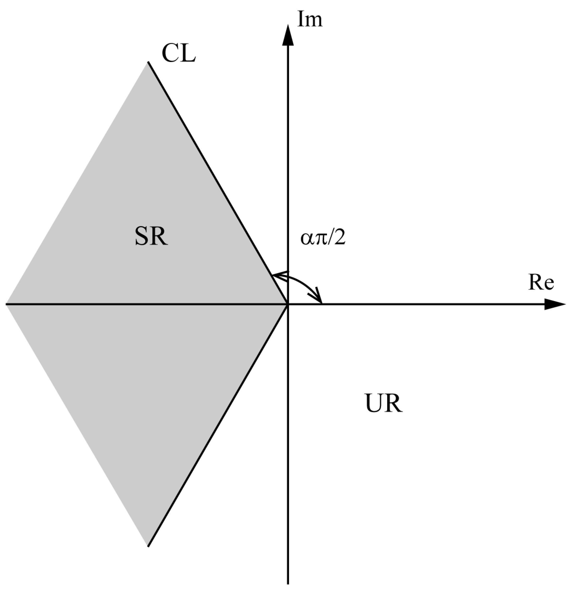
3. Main Results
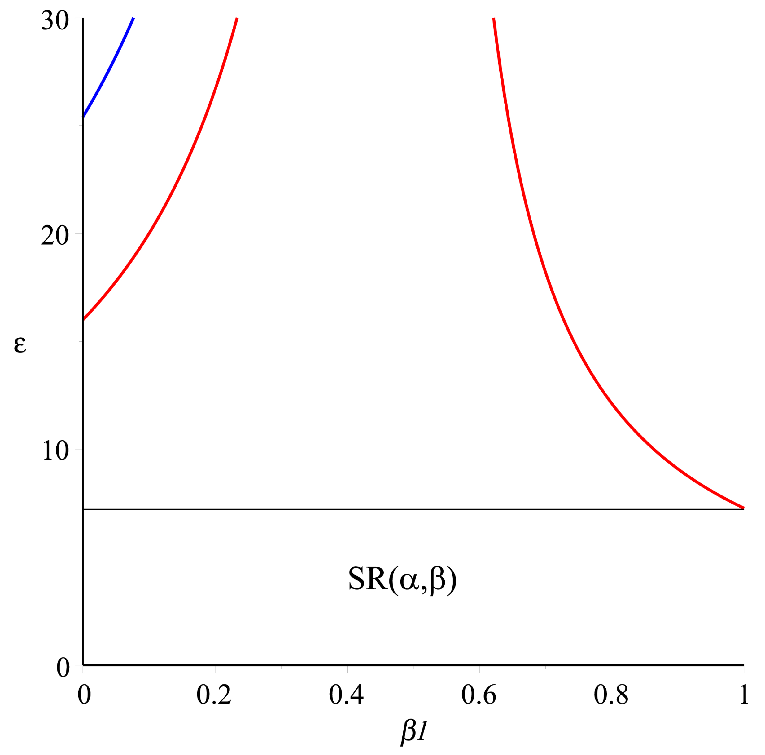
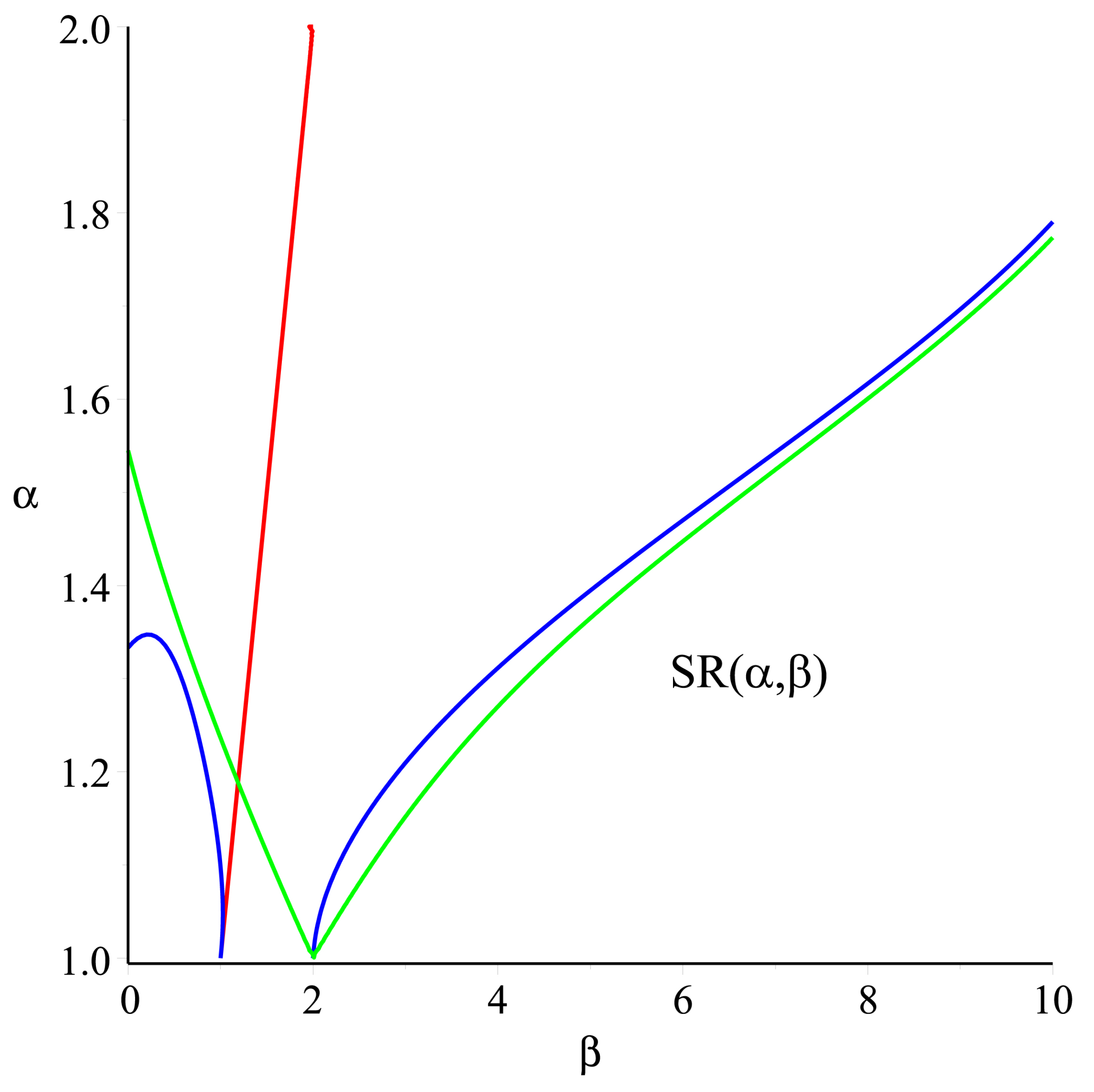
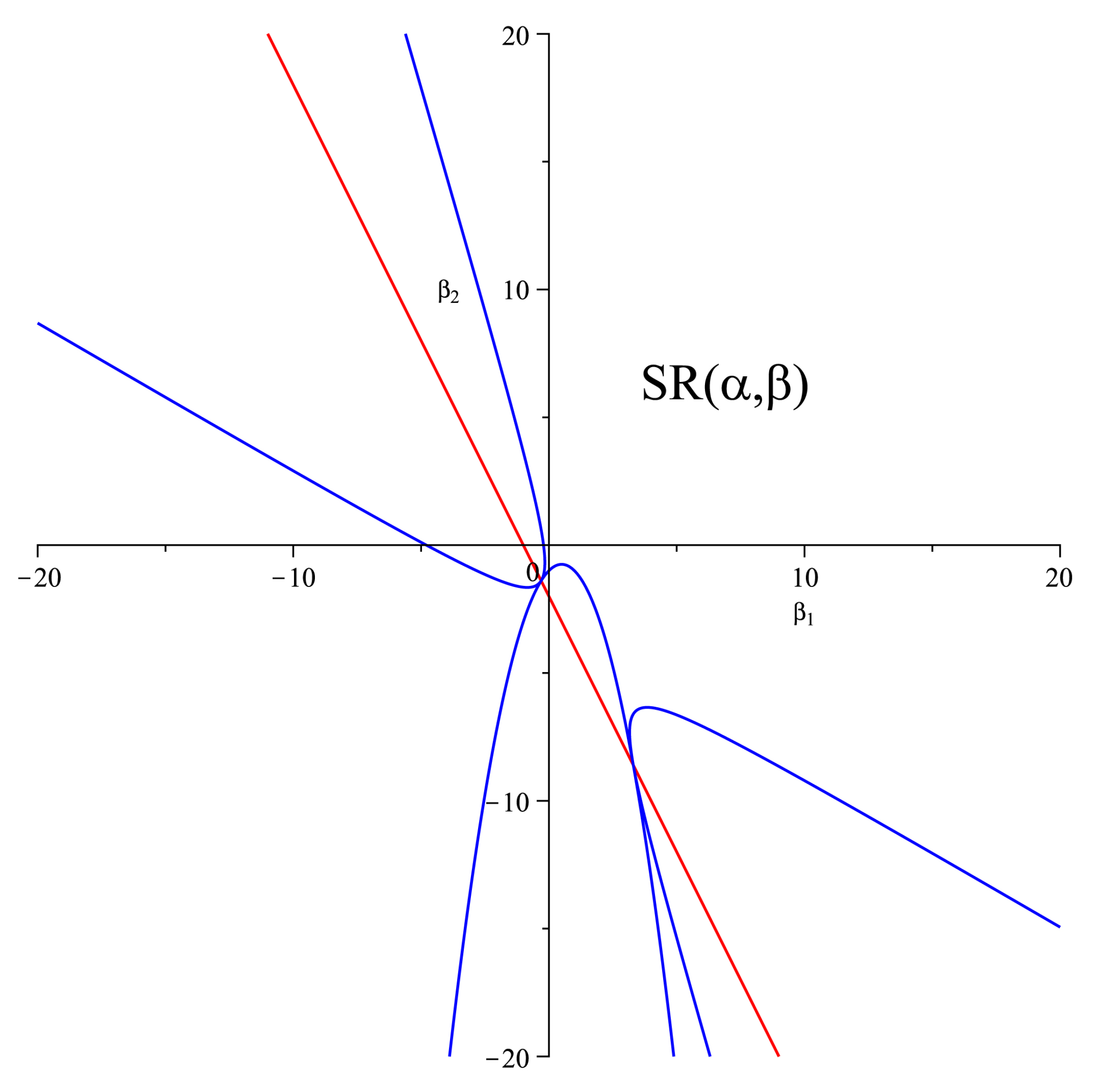
4. Illustrative Examples
5. Conclusions
Author Contributions
Funding
Institutional Review Board Statement
Informed Consent Statement
Data Availability Statement
Conflicts of Interest
Appendix A

References
- Ahmed, E.; El-Sayed, A.M.A.; El-Saka, H.A.A. On some Routh-Hurwitz conditions for fractional order differential equations and their applications in Lorenz, Rössler, Chua and Chen systems. Phys. Lett. A 2006, 1, 1–4. [Google Scholar] [CrossRef]
- Bourafa, S.; Abdelouahab, M.S.; Moussaoui, A. On some extended Routh-Hurwitz conditions for fractional-order autonomous systems of order α∈(0, 2) and their applications to some population dynamic models. Chaos Solitons Fractals 2020, 133, 109623. [Google Scholar] [CrossRef]
- Tavazoei, M.S.; Haeri, M. A note on the stability of fractional order systems. Math. Comput. Simul. 2009, 79, 1566–1576. [Google Scholar] [CrossRef]
- Lu, J.G.; Chen, Y.Q.; Cheng, W.D. Robust asymptotical stability of fractional-order linear systems with structured perturbations. Comput. Math. Appl. 2013, 66, 873–882. [Google Scholar] [CrossRef]
- Yang, J.; Hou, X.; Luo, M. A CAD-based algorithm for solving stable parameter region of fractional-order systems with structured perturbations. Fract. Calc. Appl. Anal. 2019, 22, 509–521. [Google Scholar] [CrossRef]
- Yang, J.; Hou, X. Robust bounds for fractional-order systems with uncertain order and structured perturbations via Cylindrical Algebraic Decomposition method. J. Frankl. Inst. 2019, 356, 4097–4105. [Google Scholar] [CrossRef]
- Dhayal, R.; Muslim, M. Existence and controllability of impulsive fractional stochastic differential equations driven by Rosenblatt process with Poisson jumps. J. Eng. Math. 2021, 130, 11. [Google Scholar] [CrossRef]
- Dhayal, R.; Muslim, M.; Abbas, S. Solvability and optimal controls of non-instantaneous impulsive stochastic fractional differential equation of order q ∈ 1, 2. Stochastics 2021, 93, 780–802. [Google Scholar] [CrossRef]
- Dhayal, R.; Muslim, M.; Abbas, S. Approximate and trajectory controllability of fractional stochastic differential equation with non-instantaneous impulses and Poisson jumps. Asian J. Control. 2021, 23, 2669–2680. [Google Scholar] [CrossRef]
- Dhayal, R.; Muslim, M. Approximate controllability of fractional stochastic differential equations driven by Rosenblatt process with non-instantaneous impulses. Chaos Solitons Fractals 2021, 151, 111292. [Google Scholar] [CrossRef]
- Zeng, L.; Cheng, P.; Wang, L.; Yong, W. Robust stability analysis for a class of fractional order systems with uncertain parameters. J. Frankl. Inst. 2011, 348, 1101–1113. [Google Scholar]
- Li, C.; Wang, J. Robust stability and stabilization of fractional order interval systems with coupling relationships: The 0 < α < 1 case. J. Frankl. Inst. 2012, 349, 2406–2419. [Google Scholar]
- Srivastava, H.M. Some parametric and argument variations of the operators of fractional calculus and related special functions and integral transformations. J. Nonlinear Convex Anal. 2021, 22, 1501–1520. [Google Scholar]
- Srivastava, H.M. An introductory overview of fractional-calculus operators based upon the Fox-Wright and related higher transcendental functions. J. Adv. Eng. Comput. 2021, 5, 135–166. [Google Scholar] [CrossRef]
- Kilbas, A.A.; Srivastava, H.M.; Trujillo, J.J. Theory and Applications of Fractional Differential Equations; Elsevier: Amsterdam, The Netherlands, 2006. [Google Scholar]
- Petráš, I. Fractional-Order Nonlinear Systems: Modeling, Analysis and Simulation; Springer Science and Business Media: Berlin/Heidelberg, Germany, 2011. [Google Scholar]
- Matignon, D. Stability results for fractional differential equations with applications to control processing. Comput. Eng. Syst. Appl. 1996, 2, 963–968. [Google Scholar]
- Matignon, D. Stability properties for generalized fractional differential systems. ESAIM Proc. 1998, 5, 145–158. [Google Scholar] [CrossRef]
- Boyd, S. Linear Matrix Inequalities in Systems and Control Theory; SIAM: Philadelphia, PA, USA, 1994. [Google Scholar]
- Gantmakher, F.R. The Theory of Matrices; American Mathematical Soc.: Providence, RI, USA, 2000; Volume 2. [Google Scholar]
- Ahmed, E.; El-Sayed, A.M.A.; El-Saka, H.A.A. Equilibrium points, stability and numerical solutions of fractional-order predator–prey and rabies models. J. Math. Anal. Appl. 2007, 325, 542–553. [Google Scholar] [CrossRef]
- Lu, J.G.; Chen, Y.Q. Stability and stabilization of fractional-order linear systems with convex polytopic uncertainties. Fract. Calc. Appl. Anal. 2013, 16, 142–157. [Google Scholar] [CrossRef]
- Li, X.; Wu, R. Hopf bifurcation analysis of a new commensurate fractional-order hyperchaotic system. Nonlinear Dyn. 2014, 78, 279–288. [Google Scholar] [CrossRef]

Publisher’s Note: MDPI stays neutral with regard to jurisdictional claims in published maps and institutional affiliations. |
© 2022 by the authors. Licensee MDPI, Basel, Switzerland. This article is an open access article distributed under the terms and conditions of the Creative Commons Attribution (CC BY) license (https://creativecommons.org/licenses/by/4.0/).
Share and Cite
Yang, J.; Hou, X.; Li, Y. A Generalization of Routh–Hurwitz Stability Criterion for Fractional-Order Systems with Order α ∈ (1, 2). Fractal Fract. 2022, 6, 557. https://doi.org/10.3390/fractalfract6100557
Yang J, Hou X, Li Y. A Generalization of Routh–Hurwitz Stability Criterion for Fractional-Order Systems with Order α ∈ (1, 2). Fractal and Fractional. 2022; 6(10):557. https://doi.org/10.3390/fractalfract6100557
Chicago/Turabian StyleYang, Jing, Xiaorong Hou, and Yajun Li. 2022. "A Generalization of Routh–Hurwitz Stability Criterion for Fractional-Order Systems with Order α ∈ (1, 2)" Fractal and Fractional 6, no. 10: 557. https://doi.org/10.3390/fractalfract6100557
APA StyleYang, J., Hou, X., & Li, Y. (2022). A Generalization of Routh–Hurwitz Stability Criterion for Fractional-Order Systems with Order α ∈ (1, 2). Fractal and Fractional, 6(10), 557. https://doi.org/10.3390/fractalfract6100557