Improved Results on Finite-Time Passivity and Synchronization Problem for Fractional-Order Memristor-Based Competitive Neural Networks: Interval Matrix Approach

Abstract

This research paper deals with the passivity and synchronization problem of fractional-order memristor-based competitive neural networks (FOMBCNNs) for the first time. Since the FOMBCNNs’ parameters are state-dependent, FOMBCNNs may exhibit unexpected parameter mismatch when different initial conditions are chosen. Therefore, the conventional robust control scheme cannot guarantee the synchronization of FOMBCNNs. Under the framework of the Filippov solution, the drive and response FOMBCNNs are first transformed into systems with interval parameters. Then, the new sufficient criteria are obtained by linear matrix inequalities (LMIs) to ensure the passivity in finite-time criteria for FOMBCNNs with mismatched switching jumps. Further, a feedback control law is designed to ensure the finite-time synchronization of FOMBCNNs. Finally, three numerical cases are given to illustrate the usefulness of our passivity and synchronization results.

1. Introduction

In recent years, the research on competitive-type neural networks (CNNs) has attracted expanding consideration from mathematicians, engineers, physicists and scholars. There are two forms of state variables: short-term memory and long-term memory. They make a good application background in convex optimization, cybernetics, image recognition and associative memory. Recently, many significant results on the dynamics of different kinds of neural networks, especially recurrent neural networks [1], cellular neural networks [2], T-S fuzzy neural networks [3], BAM neural networks [4] and competitive neural networks [5,6,7,8] have been obtained, but these results are mainly discussed in integer-order cases. However, there are few results focused on CNNs with fractional-order cases, see [9,10,11,12,13].

As the fourth circuit component along with resistor, capacitor and inductor, memristor was firstly postulated by Professor Chua in 1971 [14]. A resistor describes the voltage–current relationship, a capacitor depicts the charge–voltage relationship and an inductor displays the flux–current relationship. Chua showed the missing flux–charge relationship, which he named memristance and is the value of a memristor. The Hewlett-Packard laboratory fabricated a practically working memristor device in 2008 [15]. Good features of memristors such as nanometer size, nonvolatility and nonlinearity make them more suitable for simulating synapses resistors in network models. If the resistor of self-feedback connections weights is instead modeled by a memristor in conventional neural networks model, then memristor-based neural networks (MNNs) can be reached. Many interesting results on the dynamics of memristor-based neural networks have recently been proposed and studied [16,17,18,19]. Currently, many researchers also claim that MNNs provide more memory storage than conventional neural networks [20]. Undoubtedly, memristor-based competitive neural networks will advantage the associative memory capability of neural networks. It is very significant to analyze the memristor-based competitive neural networks’ dynamical behaviors.

As far back as the 1695s, the idea of fractional calculus [21] was discussed by Gottfried Wilhelm Leibniz. Comparing with traditional integer-order calculus, fractional calculus has unlimited memory property. Recently, fractional calculus has played a vital role in the science and engineering fields [22,23], and lots of scientific results have been reported on this topic, see [24,25,26,27,28]. At present, there is a trend to utilize fractional differential techniques to study the dynamics of networks, especially neural networks [29,30,31,32]. It should be mentioned that the memristance of the memristor has a fractional order. Therefore, it has been very common and precise to utilize fractional differential techniques for studying the dynamics of memristor-based neural network systems. Recently, an ever-increasing number of specialists have talked about memristor-based neural network systems with fractional order (MNNWFO) and some significant outcomes have been accounted for on stability [33,34], stabilization [35,36] and state estimation [37,38].

Passivity can keep a system internally stable, which helps to understand the stability of different dynamical systems and their properties. Recently, the research on passivity analysis has become a hot research subject and it has been effectively applied to different fields such as control systems, power systems and robot systems. In view of the energy theory, the systems have been described as well as their Lyapunov-related input/output information. In light of the Lyapunov theory, there have been numerous scientific results in the literature, see [39,40,41,42,43,44,45,46]. On the other hand, synchronization has already emerged as a hot research theme and some meaningful scientific results on MNNWFO have been obtained, see [47,48].

Since the life spans of machines and human beings are finite, asymptotic synchronization is inapplicable in practice. In this regard, the finite-time synchronization of nonlinear systems has been comprehensively investigated in the literature [49,50,51,52]. For example, the authors in [53] have analyzed the Mittag–Leffler synchronization in finite-time criteria Caputo fractional-order memristor-based BAM neural networks with fractional orders $0<\xi <1$ and $1<\xi <2$, by means of a linear feedback control law, and the generalized Gronwall inequality. On the other hand, the finite-time passivity theory can provide a powerful tool to analyze the dynamics of fractional-order neural networks. Meanwhile, to our knowledge, few published research works exist concerning this problem. To mention a few, the authors in [54] have established the robust passivity criterion of interval-parameter-based neural networks with a Caputo fractional-order derivative via passivity theory, Lyapunov theory and LMI techniques. Unfortunately, the passivity and synchronization of FOMCNNS have not been investigated yet and this situation motivates further investigation of FOMBCNNs.

Motivated by the aforementioned issues, this paper aims at analyzing the finite-time passivity and finite-time synchronization criterion of FOMBCNNs. The novelty of this manuscript is summarized as follows. (1) As far as we know, this paper is the first attempt to address the finite-time passivity and finite-synchronization for fractional-order competitive neural networks. (2) The problem addressed in this paper is described by a class of robust analytical techniques. (3) To obtain our main results, finite-time boundedness, finite-time passivity and finite-time synchronization definitions are presented. (4) In light of these definitions, several results are established theoretically. (5) These theoretical results and techniques are improved compared to the existing passivity and synchronization results of fractional-order neural networks. The remaining structure of this research work is outlined as follows: basic results on fractional-order calculus and a description of FOMBCNN systems are formally introduced in the next section. Section 3 and Section 4 describe the main results of this research paper. Section 5 yields numerical results and their simulations. Finally, Section 6 ends with conclusions.

2. System Description and Preliminaries

For a real matrix U, ${\Lambda }_{min}\left(U\right)$ and ${\Lambda }_{max}\left(U\right)$ signify the maximal and the minimal eigenvalue of U, respectively. The superscript T indicates the matrix transposition. For all $u\ne 0$, the matrix $\mathcal{H}$ is positive definite if $u^T\mathcal{H}u>0$. $\mathcal{H}>\mathbb{H}$ means $\mathcal{H}-\mathbb{H}>0$. I is the identity matrix. The symmetric term in a matrix is displayed by ★. $\mathcal{K}\left(U\right)$ stands for the closure of the convex hull of U. For $\beta \left(t\right)={({\beta }_1\left(t\right),...,{\beta }_n\left(t\right))}^T\in {\mathbb{R}}^n$, we denote

$$\begin{array}{c}\hfill {\parallel \beta \left(t\right)\parallel }_2=\sqrt{\sum _{j=1}^n{\beta }_j^2\left(t\right)}.\end{array}$$

2.1. Preliminaries

This section comprises the rudimentary definitions and lemmas, which are further employed in the subsequent section.

Definition 1.

The fractional-order integral of function $\beta \left(t\right)$ is [21]:

$$\begin{array}{c}\hfill {}_0{\mathcal{D}}_t^{-\xi }\beta \left(t\right)=\frac{1}{\Gamma \left(\xi \right)}{\int }_{t_0}^t{(t-\ell )}^{\xi -1}\beta (\ell )\mathrm{d}\ell ,\end{array}$$

where $\Gamma (·)$ is the gamma function.

Definition 2.

The Caputo fractional-order derivative of function $\beta \left(t\right)$ is [21]:

$$\begin{array}{c}\hfill {}_0^C{\mathcal{D}}_t^{\xi }\beta \left(t\right)=\frac{1}{\Gamma (n-\xi )}{\int }_{t_0}^t\frac{{\beta }^{\left(n\right)}(\ell )}{{(t-\ell )}^{\xi -n+1}}\mathrm{d}\ell ,\end{array}$$

where $t\ge t_0$ and $n-1<\xi <n\in {\mathbb{Z}}^{+}$.

Definition 3.

The Mittag–Leffler function with two parameter is described as [21]:

$$\begin{array}{c}\hfill E_{{\xi }_1,{\xi }_2}(\ell )=\sum _{i=0}^{+\infty }\frac{{\ell }^i}{\Gamma ({\xi }_{1}i+{\xi }_2)},\end{array}$$

where ${\xi }_1,{\xi }_2\in {\mathbb{R}}^{+}$ and $\ell \in \mathbb{C}$. For ${\xi }_2=1$, its Mittag–Leffler function with one parameter is displayed as

$$\begin{array}{c}\hfill E_{{\xi }_1,1}(\ell )=\sum _{i=0}^{+\infty }\frac{{\ell }^i}{\Gamma ({\xi }_{1}i+1)}=E_{{\xi }_1}(\ell ).\end{array}$$

Lemma 1.

If $\beta \left(t\right)\in C^n[0,+\infty )$ and $n-1<\xi <n,(n\in {\mathbb{Z}}^{+},n\ge 1)$, then [21]

$$\begin{array}{c}\hfill {}_0{\mathcal{D}}_t^{-\xi }\left({}_0^C{\mathcal{D}}_t^{\xi }\beta \left(t\right)\right)=\beta \left(t\right)-\sum _{u=0}^{n-1}\frac{t^u}{u!}{\beta }^u\left(t_0\right).\end{array}$$

In particular, if $0<\xi <1$, then ${}_0{\mathcal{D}}_t^{-\xi }\left({}_0^C{\mathcal{D}}_t^{\xi }\beta \left(t\right)\right)=\beta \left(t\right)-\beta \left(t_0\right)$.

Lemma 2.

For $0<\xi <1$, function $p\left(t\right)$ is continuous and is defined on $[0,+\infty )$, then there exist constants ${\varrho }_1>0$ and ${\varrho }_2\ge 0$ such that [31]

$$\begin{array}{c}\hfill {}_0^C{\mathcal{D}}_t^{\xi }p\left(t\right)\le -{\varrho }_{1}p\left(t\right)+{\varrho }_2,t\ge t_0,\end{array}$$

then

$$\begin{array}{c}\hfill p\left(t\right)\le p\left(0\right)E_{\xi }\left(-{\varrho }_1{t}^{\xi }\right)+{\varrho }_2{t}^{\xi }{E}_{\xi ,\xi +1}\left(-{\varrho }_1{t}^{\xi }\right),t\ge t_0.\end{array}$$

Lemma 3.

Let $p\left(t\right)\in {\mathbb{R}}^n$ be a continuously differentiable vector-valued function, then for any $t\ge t_0$ [32]

$$\begin{array}{c}\hfill {}_0^C{\mathcal{D}}_t^{\xi }\left\{p^T\left(t\right)\mathcal{H}p\left(t\right)\right\}\le 2p^T\left(t\right)\mathcal{H}\left\{{\mathcal{D}}_t^{\xi }p\left(t\right)\right\},\xi \in (0,1),\end{array}$$

where $\mathcal{H}\in {\mathbb{R}}^{n\times n}$ is a positive definite symmetric matrix.

2.2. Model Description

We consider a fractional-order memristor-based competitive neural network (FOMBCNN) in this manuscript:

$$\begin{array}{c}\hfill \left\{\begin{array}{c}{}_0^C{\mathcal{D}}_t^{\xi }{u}_j\left(t\right)=-p_j{u}_j\left(t\right)+\sum _{k=1}^n{q}_{jk}\left(u_j\left(t\right)\right)g_k\left(u_k\left(t\right)\right)+s_j\sum _{i=1}^m{\delta }_{ji}\left(t\right){\zeta }_i+{\pi }_f{x}_j\left(t\right)\hfill \\ {}_0^C{\mathcal{D}}_t^{\xi }{\delta }_{ji}\left(t\right)=-a_j{\delta }_{ji}\left(t\right)+{\zeta }_i{b}_j{g}_j\left(u_j\left(t\right)\right)+{\theta }_f{y}_j\left(t\right),f=1,2,...,d,\hfill \end{array}\right.\end{array}$$

(1)

where ${}_0^C{\mathcal{D}}_t^{\xi }$ signifies the Caputo derivative with order $0<\xi <1$, $u_j\left(t\right)$ represents the state variables; the current activity level is represented by $p_j$; $a_j$ and $b_j$ signifies the disposable scaling positive scalars; $g_k(·)$ represents the neuron activations; ${\delta }_{ji}$ signifies the synaptic efficiency; the weights of the external stimulus is denoted by $s_j$; $\zeta ={({\zeta }_1,...,{\zeta }_n)}^T$ represents the constant external stimulus; $x_j\left(t\right)$ and $y_j\left(t\right)$ are disturbing input vectors; ${\pi }_f$ and ${\theta }_f$ are known scalars; the synaptic memristor-based connection weights satisfy

$$\begin{array}{ccc}\hfill q_{jk}\left(u_j\left(t\right)\right)& =& \left\{\begin{array}{cc}{\widehat{q}}_{jk},\hfill & |u_j\left(t\right)|\le {\mathcal{I}}_j\hfill \\ {\breve{q}}_{jk},\hfill & |u_j\left(t\right)|>{\mathcal{I}}_j,\hfill \end{array}\right.\hfill \end{array}$$

in which ${\mathcal{I}}_j>0$ are switching jumps and ${\widehat{q}}_{jk}>0,{\breve{q}}_{jk}>0$ are constants.

Define $w_j\left(t\right)={\sum }_{i=1}^m{\delta }_{ji}\left(t\right){\zeta }_i=\zeta {\delta }_j^T\left(t\right),j=1,2,...,n$, where ${\delta }_j(·)={[{\delta }_{j1}(·),...,{\delta }_{jm}(·)]}^T$. Then, the transformation system (1) can be written as

$$\begin{array}{c}\hfill \left\{\begin{array}{c}{}_0^C{\mathcal{D}}_t^{\xi }{u}_j\left(t\right)=-p_j{u}_j\left(t\right)+\sum _{k=1}^n{q}_{jk}\left(u_j\left(t\right)\right)g_k\left(u_k\left(t\right)\right)+s_j{w}_j\left(t\right)+{\pi }_f{x}_j\left(t\right)\hfill \\ {}_0^C{\mathcal{D}}_t^{\xi }{w}_j\left(t\right)=-a_j{w}_j\left(t\right)+{\left|{\zeta }_i\right|}^2{b}_j{g}_j\left(u_j\left(t\right)\right)+{\theta }_f{y}_j\left(t\right),f=1,2,...,d,\hfill \end{array}\right.\end{array}$$

(2)

where $|{\zeta }_i{|}^2={\zeta }_1^2+...+{\zeta }_m^2$ is scalar. Without loss of generality, the input stimulus vector is supposed to be normalized with unit magnitude $|{\zeta }_i{|}^2=1$. Then, the above equation can be written as

$$\begin{array}{c}\hfill \left\{\begin{array}{c}{}_0^C{\mathcal{D}}_t^{\xi }{u}_j\left(t\right)=-p_j{u}_j\left(t\right)+\sum _{k=1}^n{q}_{jk}\left(u_j\left(t\right)\right)g_k\left(u_k\left(t\right)\right)+s_j{w}_j\left(t\right)+{\pi }_f{x}_j\left(t\right)\hfill \\ {}_0^C{\mathcal{D}}_t^{\xi }{w}_j\left(t\right)=-a_j{w}_j\left(t\right)+b_j{g}_j\left(u_j\left(t\right)\right)+{\theta }_f{y}_j\left(t\right),f=1,2,...,d.\hfill \end{array}\right.\end{array}$$

(3)

Remark 1.

The memristor-based connection weights of the system are changed based on the system state. Therefore, FOMBCNN (1) can be regarded as a state-dependent switching system, which is a special case of the dynamics of competitive neural networks.

Define $q_{jk}^{+}=max\left\{{\widehat{q}}_{jk},{\breve{q}}_{jk}\right\}$, $q_{jk}^{-}=min\left\{{\widehat{q}}_{jk},{\breve{q}}_{jk}\right\}$, ${\stackrel{`}{q}}_{jk}=\frac{1}{2}\left(q_{jk}^{+}+q_{jk}^{-}\right)$ and ${\acute{q}}_{jk}=\frac{1}{2}\left(q_{jk}^{+}-q_{jk}^{-}\right)$. Then, FOMBCNN (1) can be written in the following form:

$$\begin{array}{c}\hfill \left\{\begin{array}{c}{}_0^C{\mathcal{D}}_t^{\xi }{u}_j\left(t\right)=-p_j{u}_j\left(t\right)+\sum _{k=1}^n\left({\stackrel{`}{q}}_{jk}+{\Delta }_{jk}\left(u_j\left(t\right)\right)\right)g_k\left(u_k\left(t\right)\right)+s_j{w}_j\left(t\right)+{\pi }_f{x}_j\left(t\right)\hfill \\ {}_0^C{\mathcal{D}}_t^{\xi }{w}_j\left(t\right)=-a_j{w}_j\left(t\right)+b_j{g}_j\left(u_j\left(t\right)\right)+{\theta }_f{y}_j\left(t\right),f=1,2,...,d,\hfill \end{array}\right.\end{array}$$

(4)

where

$$\begin{array}{ccc}\hfill {\Delta }_{jk}\left(u_j\left(t\right)\right)& =& \left\{\begin{array}{cc}{\acute{q}}_{jk},\hfill & q_{jk}\left(u_j\left(t\right)\right)=q_{jk}^{+}\hfill \\ -{\acute{q}}_{jk},\hfill & q_{jk}\left(u_j\left(t\right)\right)=q_{jk}^{-}.\hfill \end{array}\right.\hfill \end{array}$$

Based on Filippov’s theory [55] and some transformation techniques, it can be obtained from (4) that

$$\begin{array}{c}\hfill \left\{\begin{array}{c}{}_0^C{\mathcal{D}}_t^{\xi }{u}_j\left(t\right)\in -p_j{u}_j\left(t\right)+\sum _{k=1}^n\left({\stackrel{`}{q}}_{jk}+\mathcal{K}\left[-{\acute{q}}_{jk},{\acute{q}}_{jk}\right]\right)g_k\left(u_k\left(t\right)\right)+s_j{w}_j\left(t\right)+{\pi }_f{x}_j\left(t\right)\hfill \\ {}_0^C{\mathcal{D}}_t^{\xi }{w}_j\left(t\right)=-a_j{w}_j\left(t\right)+b_j{g}_j\left(u_j\left(t\right)\right)+{\theta }_f{y}_j\left(t\right),f=1,2,...,d,\hfill \end{array}\right.\end{array}$$

(5)

According to the measurable selection theorem [56], there exists a measurable function ${\chi }_{jk}\left(t\right)\in \mathcal{K}[-1,1]$ such that

$$\begin{array}{c}\hfill \left\{\begin{array}{c}{}_0^C{\mathcal{D}}_t^{\xi }{u}_j\left(t\right)=-p_j{u}_j\left(t\right)+\sum _{k=1}^n\left[{\stackrel{`}{q}}_{jk}+{\acute{q}}_{jk}{\chi }_{jk}\left(t\right)\right]g_k\left(u_k\left(t\right)\right)+s_j{w}_j\left(t\right)+{\pi }_f{x}_j\left(t\right)\hfill \\ {}_0^C{\mathcal{D}}_t^{\xi }{w}_j\left(t\right)=-a_j{w}_j\left(t\right)+b_j{g}_j\left(u_j\left(t\right)\right)+{\theta }_f{y}_j\left(t\right),f=1,2,...,d.\hfill \end{array}\right.\end{array}$$

(6)

Throughout this manuscript, we make the following assumptions.

$\left(\mathbf{A}\mathbf{1}\right)$. The nonlinear feedback function $g_k$ is bounded and satisfies:

$$\begin{array}{ccc}\hfill 0& \le & \frac{g_k\left({\gamma }_1\right)-g_k\left({\gamma }_2\right)}{{\gamma }_1-{\gamma }_2}\le l_k,k=1,2,...,n,\forall {\gamma }_1\ne {\gamma }_2\in \mathbb{R},\hfill \end{array}$$

where $l_k>0(k=1,2,...,n)$ are scalars.

$\left(\mathbf{A}\mathbf{2}\right)$. The disturbance input $x\left(t\right)={[x_1\left(t\right),...,x_n\left(t\right)]}^T,y\left(t\right)={[x_1\left(t\right),...,x_n\left(t\right)]}^T\in {\mathbb{R}}^n$ are time varying, and there exist constants ${\lambda }_1>0$ and ${\lambda }_2>0$ such that the disturbance input vectors fulfills the following relationships:

$$\begin{array}{c}\hfill x^T\left(t\right)x\left(t\right)\le {\lambda }_1,y^T\left(t\right)y\left(t\right)\le {\lambda }_2.\end{array}$$

In the development of the main results, the following lemmas are significant.

Lemma 4.

[57] Let ${\zeta }_1>0,{\zeta }_2>0,{\zeta }_3>1,{\zeta }_4>1$ and ${\zeta }_3^{-1}+{\zeta }_4^{-1}=1$, then the following inequality is fulfilled:

$$\begin{array}{c}\hfill {\zeta }_1{\zeta }_2\le \frac{{\left(\eta {\zeta }_1\right)}^{{\zeta }_3}}{{\zeta }_3}+\frac{{\left({\eta }^{-1}{\zeta }_2\right)}^{{\zeta }_4}}{{\zeta }_4}\end{array}$$

where $\eta >0$ is a constant.

Lemma 5.

[58] Given matrices $\mathcal{H}={\mathcal{H}}^T$, $\mathcal{E},\mathcal{G}$ and $\mathcal{M}={\mathcal{M}}^T>0$ of appropriate dimension,

$$\begin{array}{c}\hfill \mathcal{H}+\mathcal{E}\Phi \mathcal{G}+{\mathcal{G}}^T{\Phi }^T{\mathcal{G}}^T<0,\end{array}$$

for all ${\Phi }^T\Phi \le \mathcal{M}$, if and only if there exists some $\beta >0$ such that

$$\begin{array}{c}\hfill \mathcal{H}+\beta \mathcal{E}{\mathcal{E}}^T+{\beta }^{-1}{\mathcal{G}}^T\mathcal{M}\mathcal{G}<0.\end{array}$$

Lemma 6.

[59] Let $\alpha >0$, for any ${\Re }_1,{\Re }_2\in {\mathbb{R}}^n$ and $n\times n$ matrix $\mathcal{H}$,

$$\begin{array}{ccc}\hfill {\Re }_1^T\mathcal{H}{\Re }_2& \le & \frac{{\alpha }^{-1}}{2}{\Re }_1^T\mathcal{H}{\mathcal{H}}^T{\Re }_1+\frac{\alpha }{2}{\Re }_2^T{\Re }_2.\hfill \end{array}$$

3. Finite-Time Passivity

In this section, we demonstrate the finite-time passivity criterion of FOMBCNN (1), which is equivalent to the FOMBCNN system (6).

First, we define the following notations:

$$\begin{array}{ccc}\hfill \mathcal{E}& =& {\left(\sqrt{{\acute{q}}_{11}}{\eta }_1,....,\sqrt{{\acute{q}}_{1n}}{\eta }_1,....,\sqrt{{\acute{q}}_{n1}}{\eta }_n,....,\sqrt{{\acute{q}}_{nn}}{\eta }_n\right)}_{n\times n^2}\hfill \\ \hfill \mathcal{G}& =& {\left(\sqrt{{\acute{q}}_{11}}{\eta }_1,....,\sqrt{{\acute{q}}_{1n}}{\eta }_n,....,\sqrt{{\acute{q}}_{n1}}{\eta }_1,....,\sqrt{{\acute{q}}_{nn}}{\eta }_n\right)}_{n^2\times n}^T,\hfill \end{array}$$

(7)

${\eta }_j\in {\mathbb{R}}^n$, the j-th element of ${\eta }_j$ is one and all others are zero. From (7), one has

$$\begin{array}{ccc}\hfill {\mathcal{Q}}_1& =& \mathcal{E}{\mathcal{E}}^T=diag\left\{\sum _{k=1}^n{\acute{q}}_{1k},...,\sum _{k=1}^n{\acute{q}}_{nk}\right\},\hfill \\ \hfill {\mathcal{Q}}_2& =& \mathcal{G}{\mathcal{G}}^T=diag\left\{\sum _{k=1}^n{\acute{q}}_{k1},...,\sum _{k=1}^n{\acute{q}}_{kn}\right\}.\hfill \end{array}$$

(8)

Let us also denote

$$\begin{array}{c}\hfill {\left[\mathcal{N}\left(t\right)\right]}_{n^2\times n^2}=\left\{diag\left\{{\chi }_{11}\left(t\right),....,{\chi }_{1n}\left(t\right),...,{\chi }_{n1}\left(t\right),....,{\chi }_{nn}\left(t\right)\right\},\left|{\chi }_{jk}\right|\le 1,1\le j,k\le n\right\}.\end{array}$$

Obviously, ${\mathcal{N}}^T\left(t\right)\mathcal{N}\left(t\right)\le 1$. The vector form of FOMBCNN (6) can be written as:

$$\begin{array}{c}\hfill \left\{\begin{array}{c}{}_0^C{\mathcal{D}}_t^{\xi }u\left(t\right)=-\mathcal{P}u\left(t\right)+\left(\mathcal{Q}+\mathcal{E}\mathcal{N}\left(t\right)\mathcal{G}\right)g\left(u\left(t\right)\right)+\mathcal{S}w\left(t\right)+\mathcal{F}x\left(t\right)\hfill \\ {}_0^C{\mathcal{D}}_t^{\xi }w\left(t\right)=-\mathcal{A}w\left(t\right)+\mathcal{B}g\left(u\left(t\right)\right)+\mathcal{H}y\left(t\right),\hfill \end{array}\right.\end{array}$$

(9)

where $\mathcal{P}=diag\{p_1,...,p_n\}\in {\mathbb{R}}^n,$$\mathcal{Q}=\left({\stackrel{`}{q}}_{jk}\right)\in {\mathbb{R}}^{n\times n}$, $\mathcal{S}=diag\{s_1,...,s_n\}\in {\mathbb{R}}^n,$$\mathcal{A}=diag\{a_1,...,a_n\}\in {\mathbb{R}}^n,$ $\mathcal{B}=diag\{b_1,...,b_n\}\in {\mathbb{R}}^n,$$\mathcal{F}=diag\{{\pi }_1,...,{\pi }_d\}\in {\mathbb{R}}^d$ and $\mathcal{H}=diag\{{\theta }_1,...,{\theta }_d\}\in {\mathbb{R}}^d$. The measured output vector of model (9) is assumed to be:

$$\begin{array}{c}\hfill \left\{\begin{array}{c}{q}_u\left(t\right)={\mathcal{R}}_{u}u\left(t\right)\hfill \\ q_w\left(t\right)={\mathcal{R}}_{w}w\left(t\right),\hfill \end{array}\right.\end{array}$$

(10)

where $q_u\left(t\right)\in {\mathbb{R}}^d$, $q_w\left(t\right)\in {\mathbb{R}}^d$ and ${\mathcal{R}}_u,{\mathcal{R}}_w\in {\mathbb{R}}^{d\times n}$.

The following definitions are much needed to establish the finite-time passivity criteria of system (9).

Definition 4.

FOMBCNN (9) with measured output $q_u\left(t\right)=q_w\left(t\right)=0$ is finite-time bounded with respect to $\left({\sigma }_1,{\sigma }_2,T_{\sigma },{\mathcal{H}}_1,{\mathcal{H}}_2,{\lambda }_1,{\lambda }_2\right)$, where ${\mathcal{H}}_1,{\mathcal{H}}_2$ are symmetric positive definite matrices, if

$$\begin{array}{c}\hfill u^T\left(t_0\right){\mathcal{H}}_{1}u\left(t_0\right)+w^T\left(t_0\right){\mathcal{H}}_{2}w\left(t_0\right)\le {\sigma }_1\end{array}$$

implies that

$$\begin{array}{c}\hfill u^T\left(t\right){\mathcal{H}}_{1}u\left(t\right)+w^T\left(t\right){\mathcal{H}}_{2}w\left(t\right)\le {\sigma }_2,\forall t\in [t_0,T_{\sigma }],\end{array}$$

and for all $x\left(t\right)\in {\mathbb{R}}^n$ and $y\left(t\right)\in {\mathbb{R}}^n$ Assumption $\left(\mathbf{A}\mathbf{2}\right)$ is held.

Definition 5.

FOMBCNN (9) is finite-time passive with respect to $\left({\sigma }_1,{\sigma }_2,T_{\sigma },{\mathcal{H}}_1,{\mathcal{H}}_2,{\lambda }_1,{\lambda }_2\right)$, where ${\mathcal{H}}_1,{\mathcal{H}}_2$ are symmetric positive definite matrices, if the following relationship holds:

1.

When measured output $q_u\left(t\right)=q_w\left(t\right)=0$, FOMBCNN (9) is finite-time bounded with respect to $\left({\sigma }_1,{\sigma }_2,T_{\sigma },{\mathcal{H}}_1,{\mathcal{H}}_2,{\lambda }_1,{\lambda }_2\right)$.

2.

Under the zero initial values, there exists a constant $\upsilon >0$ such that

$$\begin{array}{c}\hfill 2{}_0^C{\mathcal{D}}_t^{-\xi }\left[q_u\left(t\right)x\left(t\right)+q_w\left(t\right)y\left(t\right)\right]\ge -\upsilon {}_0^C{\mathcal{D}}_t^{-\xi }\left[x^T\left(t\right)x\left(t\right)+y^T\left(t\right)y\left(t\right)\right],\forall t\in [t_0,T_{\sigma }].\end{array}$$

Theorem 1.

Suppose that Assumptions $\left(\mathbf{A}\mathbf{1}\right)$ and $\left(\mathbf{A}\mathbf{2}\right)$ hold. FOMBCNN (1) with measured output $q_u\left(t\right)=q_w\left(t\right)=0$ is finite-time bounded with respect to $\left({\sigma }_1,{\sigma }_2,T_{\sigma },{\mathcal{H}}_1,{\mathcal{H}}_2,{\lambda }_1,{\lambda }_2\right)$, if there exist symmetric positive definite matrices ${\mathcal{H}}_1$, a positive diagonal matrix ${\mathcal{H}}_2$ and positive constants ${\alpha }_i,i=1,2,3,4,5$ and $\beta >0$ such that

$$\begin{array}{ccc}\hfill \Phi & =& \left[\begin{array}{ccccc}{\Phi }_1& {\mathcal{H}}_1\mathcal{Q}& {\mathcal{H}}_1\mathcal{S}& {\mathcal{H}}_1\mathcal{F}& {\mathcal{H}}_1\sqrt{{\mathcal{Q}}_1}\\ ★& -{\alpha }_{1}I+\beta {\mathcal{Q}}_2& 0& 0& 0\\ ★& ★& -{\alpha }_{2}I& 0& 0\\ ★& ★& ★& -{\alpha }_{3}I& 0\\ ★& ★& ★& ★& -\beta I\end{array}\right]<0\hfill \end{array}$$

(11)

$$\begin{array}{ccc}\hfill \Psi & =& \left[\begin{array}{ccc}-{\mathcal{H}}_2\mathcal{A}-{\mathcal{A}}^T{\mathcal{H}}_2+{\alpha }_{2}I& {\mathcal{H}}_2\mathcal{B}& {\mathcal{H}}_2\mathcal{H}\\ ★& -{\alpha }_{4}I& 0\\ ★& ★& -{\alpha }_{5}I\end{array}\right]<0\hfill \end{array}$$

(12)

$$\begin{array}{ccc}\hfill \underline{\vartheta }{\sigma }_2& >& \overline{\vartheta }{\sigma }_1+\frac{\alpha ({\lambda }_1+{\lambda }_2)}{\Gamma (\xi +1)}{T}_{\sigma }^{\xi },\hfill \end{array}$$

(13)

where ${\Phi }_1=-{\mathcal{H}}_1\mathcal{P}-{\mathcal{P}}^T{\mathcal{H}}_1+[{\alpha }_1+{\alpha }_4]{\mathcal{L}}^T\mathcal{L}$, ${\mathbb{H}}_1={\mathcal{H}}_1^{-\frac{1}{2}}{\mathcal{H}}_1{\mathcal{H}}_1^{-\frac{1}{2}}$, ${\mathbb{H}}_2={\mathcal{H}}_2^{-\frac{1}{2}}{\mathcal{H}}_2{\mathcal{H}}_2^{-\frac{1}{2}}$, $\underline{\vartheta }=min\{{\Lambda }_{min}\left({\mathbb{H}}_1\right),{\Lambda }_{min}\left({\mathbb{H}}_2\right)\}$, $\overline{\vartheta }=max\{{\Lambda }_{max}\left({\mathbb{H}}_1\right),{\Lambda }_{max}\left({\mathbb{H}}_2\right)\}$ and $\alpha =max\{{\alpha }_1,{\alpha }_2\}$.

Proof. 

Define the following functional for FOMBCNN (9) as

$$\begin{array}{c}\hfill W(u\left(t\right),w\left(t\right))=u^T\left(t\right){\mathcal{H}}_{1}u\left(t\right)+w^T\left(t\right){\mathcal{H}}_{2}w\left(t\right).\end{array}$$

(14)

According to Lemma 3, we have

$$\begin{array}{ccc}\hfill {}_0^C{\mathcal{D}}_t^{\xi }W(u\left(t\right),w\left(t\right))& \le & 2u^T\left(t\right){\mathcal{H}}_1{\{}_0^C{\mathcal{D}}_t^{\xi }u\left(t\right)\}+2w^T\left(t\right){\mathcal{H}}_2{\{}_0^C{\mathcal{D}}_t^{\xi }w\left(t\right)\}\hfill \\ & =& 2u^T\left(t\right){\mathcal{H}}_1\left[-\mathcal{P}u\left(t\right)+\mathbb{Q}g\left(u\left(t\right)\right)+\mathcal{S}w\left(t\right)+\mathcal{F}x\left(t\right)\right]\hfill \\ \hfill & & +2w^T\left(t\right){\mathcal{H}}_2\left[-\mathcal{A}w\left(t\right)+\mathcal{B}g\left(u\left(t\right)\right)+\mathcal{H}y\left(t\right)\right]\hfill \\ & =& u^T\left(t\right)\left[-{\mathcal{H}}_1\mathcal{P}-{\mathcal{P}}^T{\mathcal{H}}_1\right]u\left(t\right)+2u^T\left(t\right){\mathcal{H}}_1\mathbb{Q}g\left(u\left(t\right)\right)\hfill \\ \hfill & & +2u^T\left(t\right){\mathcal{H}}_1\mathcal{S}w\left(t\right)+2u^T\left(t\right){\mathcal{H}}_1\mathcal{F}x\left(t\right)\hfill \\ \hfill & & +w^T\left(t\right)\left[-{\mathcal{H}}_2\mathcal{A}-{\mathcal{A}}^T{\mathcal{H}}_2\right]w\left(t\right)\hfill \\ \hfill & & +2w^T\left(t\right){\mathcal{H}}_2\mathcal{B}g\left(u\left(t\right)\right)+2w^T\left(t\right){\mathcal{H}}_2\mathcal{H}y\left(t\right),\hfill \end{array}$$

(15)

where $\mathbb{Q}=\mathcal{Q}+\mathcal{E}\mathcal{N}\left(t\right)\mathcal{G}$. Based on Lemma 6, we obtain

$$\begin{array}{ccc}\hfill {}_0^C{\mathcal{D}}_t^{\xi }W(u\left(t\right),w\left(t\right))& \le & u^T\left(t\right)\left[-{\mathcal{H}}_1\mathcal{P}-{\mathcal{P}}^T{\mathcal{H}}_1\right]u\left(t\right)\hfill \\ \hfill & & +{\alpha }_1^{-1}{u}^T\left(t\right)\left({\mathcal{H}}_1\mathbb{Q}\right){\left({\mathcal{H}}_1\mathbb{Q}\right)}^{T}u\left(t\right)+{\alpha }_1{u}^T\left(t\right){\mathcal{L}}^T\mathcal{L}u\left(t\right)\hfill \\ \hfill & & +{\alpha }_2^{-1}{u}^T\left(t\right)\left({\mathcal{H}}_1\mathcal{S}\right){\left({\mathcal{H}}_1\mathcal{S}\right)}^{T}u\left(t\right)+{\alpha }_2{w}^T\left(t\right)w\left(t\right)\hfill \\ \hfill & & +{\alpha }_3^{-1}{u}^T\left(t\right)\left({\mathcal{H}}_1\mathcal{F}\right){\left({\mathcal{H}}_1\mathcal{F}\right)}^{T}u\left(t\right)+{\alpha }_3{x}^T\left(t\right)x\left(t\right)\hfill \\ \hfill & & +w^T\left(t\right)\left[-{\mathcal{H}}_2\mathcal{A}-{\mathcal{A}}^T{\mathcal{H}}_2\right]w\left(t\right)+{\alpha }_4^{-1}{w}^T\left(t\right)\left({\mathcal{H}}_2\mathcal{B}\right){\left({\mathcal{H}}_2\mathbb{B}\right)}^{T}w\left(t\right)\hfill \\ \hfill & & +{\alpha }_4{u}^T\left(t\right){\mathcal{L}}^T\mathcal{L}u\left(t\right)+{\alpha }_5^{-1}{w}^T\left(t\right)\left({\mathcal{H}}_2\mathcal{H}\right){\left({\mathcal{H}}_2\mathcal{H}\right)}^{T}w\left(t\right)+{\alpha }_5{y}^T\left(t\right)y\left(t\right)\hfill \\ & \le & u^T\left(t\right)\Phi u\left(t\right)+w^T\left(t\right)\Psi w\left(t\right)+{\alpha }_3{x}^T\left(t\right)x\left(t\right)+{\alpha }_5{y}^T\left(t\right)y\left(t\right),\hfill \end{array}$$

(16)

where $\mathcal{L}=diag\{l_1,...,l_n\}$ and

$$\begin{array}{ccc}\hfill \Phi & =& -{\mathcal{H}}_1\mathcal{P}-{\mathcal{P}}^T{\mathcal{H}}_1+{\alpha }_1^{-1}\left({\mathcal{H}}_1\mathbb{Q}\right){\left({\mathcal{H}}_1\mathbb{Q}\right)}^T+[{\alpha }_1+{\alpha }_4]{\mathcal{L}}^T\mathcal{L}+{\alpha }_2^{-1}\left({\mathcal{H}}_1\mathcal{S}\right){\left({\mathcal{H}}_1\mathcal{S}\right)}^T\hfill \\ \hfill & & +{\alpha }_3^{-1}\left({\mathcal{H}}_1\mathcal{F}\right){\left({\mathcal{H}}_1\mathcal{F}\right)}^T<0\hfill \end{array}$$

(17)

$$\begin{array}{ccc}\hfill \Psi & =& -{\mathcal{H}}_2\mathcal{A}-{\mathcal{A}}^T{\mathcal{H}}_2+{\alpha }_4^{-1}\left({\mathcal{H}}_2\mathcal{B}\right){\left({\mathcal{H}}_2\mathbb{B}\right)}^T+{\alpha }_5^{-1}\left({\mathcal{H}}_2\mathcal{H}\right){\left({\mathcal{H}}_2\mathcal{H}\right)}^T+{\alpha }_{2}I<0.\hfill \end{array}$$

(18)

According to the Schur complement Lemma, (18) is equivalent to LMIs (12) and (17) is equivalent to the following LMIs (19)

$$\begin{array}{ccc}\hfill \Phi & =& \left[\begin{array}{cccc}{\Phi }_1& {\mathcal{H}}_1\mathbb{Q}& {\mathcal{H}}_1\mathcal{S}& {\mathcal{H}}_1\mathcal{F}\\ ★& -{\alpha }_{1}I& 0& 0\\ ★& ★& -{\alpha }_{2}I& 0\\ ★& ★& ★& -{\alpha }_{3}I\end{array}\right]\hfill \end{array}$$

(19)

with ${\Phi }_1=-{\mathcal{H}}_1\mathcal{P}-{\mathcal{P}}^T{\mathcal{H}}_1+[{\alpha }_1+{\alpha }_4]{\mathcal{L}}^T\mathcal{L}$.

Replacing $\mathbb{Q}$ in (19) by $\mathcal{Q}+\mathcal{E}\mathcal{N}\left(t\right)\mathcal{G}$. From (19), $\Phi$ is equivalent to

$$\begin{array}{ccc}\hfill \Phi & =& \left[\begin{array}{cccc}{\Phi }_1& {\mathcal{H}}_1\mathcal{Q}& {\mathcal{H}}_1\mathcal{S}& {\mathcal{H}}_1\mathcal{F}\\ ★& -{\alpha }_{1}I& 0& 0\\ ★& ★& -{\alpha }_{2}I& 0\\ ★& ★& ★& -{\alpha }_{3}I\end{array}\right]+\left[\begin{array}{cc}{\mathcal{H}}_1\mathcal{E}& \\ 0\\ 0\\ 0\end{array}\right]\mathcal{N}\left(t\right)\left[\begin{array}{cccc}0& \mathcal{G}& 0& 0\end{array}\right]\hfill \\ \hfill & & +\left[\begin{array}{c}0\\ {\mathcal{G}}^T\\ 0\\ 0\end{array}\right]{\mathcal{N}}^T\left(t\right)\left[\begin{array}{ccccc}{\mathcal{E}}^T{\mathcal{H}}_1& 0& 0& 0& \end{array}\right]<0.\hfill \end{array}$$

(20)

Based on Lemma 5 in (20), there exists $\beta >0$ such that $\Phi <0$ is equivalent to

$$\begin{array}{ccc}\hfill \Pi & =& \left[\begin{array}{cccc}{\Phi }_1& {\mathcal{H}}_1\mathcal{Q}& {\mathcal{H}}_1\mathcal{S}& {\mathcal{H}}_1\mathcal{F}\\ ★& -{\alpha }_{1}I& 0& 0\\ ★& ★& -{\alpha }_{2}I& 0\\ ★& ★& ★& -{\alpha }_{3}I\end{array}\right]+{\beta }^{-1}\left[\begin{array}{c}{\mathcal{H}}_1\mathcal{E}\\ 0\\ 0\\ 0\end{array}\right]\left[\begin{array}{cccc}{\mathcal{E}}^T{\mathcal{H}}_1& 0& 0& 0\end{array}\right]\hfill \\ \hfill & & +\beta \left[\begin{array}{c}0\\ {\mathcal{G}}^T\\ 0\\ 0\end{array}\right]\left[\begin{array}{cccc}0& \mathcal{G}& 0& 0\end{array}\right]<0\hfill \end{array}$$

(21)

which can be rewritten as

$$\begin{array}{ccc}\hfill \Phi & =& \left[\begin{array}{cccc}{\Phi }_1+{\beta }^{-1}{\mathcal{H}}_1\mathcal{E}{\mathcal{E}}^T{\mathcal{H}}_1& {\mathcal{H}}_1\mathcal{Q}& {\mathcal{H}}_1\mathcal{S}& {\mathcal{H}}_1\mathcal{F}\\ ★& -{\alpha }_{1}I+\beta \mathcal{G}{\mathcal{G}}^T& 0& 0\\ ★& ★& -{\alpha }_{2}I& 0\\ ★& ★& ★& -{\alpha }_{3}I\end{array}\right]<0.\hfill \end{array}$$

(22)

Based on the Schur Complement Lemma, expression (22) can be rearranged as condition (11). Therefore, from conditions (11) and (12), we have

$$\begin{array}{ccc}\hfill {}_0^C{\mathcal{D}}_t^{\xi }W(u\left(t\right),w\left(t\right))& \le & \alpha [x^T\left(t\right)x+y^T\left(t\right)y\left(t\right)].\hfill \end{array}$$

(23)

Taking the fractional integration of (23) from $t_0$ to $t(t_0\le t\le T_{\sigma })$ and based on Lemma 1, one can obtain

$$\begin{array}{ccc}\hfill u^T\left(t\right){\mathcal{H}}_{1}u\left(t\right)+w^T\left(t\right){\mathcal{H}}_{2}w\left(t\right)& \le & u^T\left(t_0\right){\mathcal{H}}_{1}u\left(t_0\right)+w^T\left(t_0\right){\mathcal{H}}_{2}w\left(t_0\right)\hfill \\ \hfill & & +\frac{\alpha }{\Gamma \left(\xi \right)}{\int }_{t_0}^t{(t-\ell )}^{\xi -1}\left[x^T(\ell )x(\ell )+y^T(\ell )y(\ell )\right]d\ell \hfill \\ & \le & u^T\left(t_0\right){\mathcal{H}}_{1}u\left(t_0\right)+w^T\left(t_0\right){\mathcal{H}}_{2}w\left(t_0\right)+\frac{T_{\sigma }^{\xi }\alpha ({\lambda }_1+{\lambda }_2)}{\Gamma (\xi +1)}.\hfill \end{array}$$

(24)

On the other hand,

$$\begin{array}{ccc}\hfill u^T\left(t\right){\mathcal{H}}_{1}u\left(t\right)+w^T\left(t\right){\mathcal{H}}_{2}w\left(t\right)& =& u^T\left(t\right){\mathcal{H}}_1^{\frac{1}{2}}{\mathbb{H}}_1{\mathcal{H}}_1^{\frac{1}{2}}u\left(t\right)+w^T\left(t\right){\mathcal{H}}_2^{\frac{1}{2}}{\mathbb{H}}_2{\mathcal{H}}_2^{\frac{1}{2}}w\left(t\right)\hfill \\ & \ge & {\Lambda }_{min}\left({\mathbb{H}}_1\right)u^T\left(t\right){\mathcal{H}}_{1}u\left(t\right)+{\Lambda }_{min}\left({\mathbb{H}}_2\right)w^T\left(t\right){\mathcal{H}}_{2}w\left(t\right)\hfill \\ & =& \underline{\vartheta }\left[u^T\left(t\right){\mathcal{H}}_{1}u\left(t\right)+w^T\left(t\right){\mathcal{H}}_{2}w\left(t\right)\right],\hfill \end{array}$$

(25)

and

$$\begin{array}{ccc}\hfill u^T\left(t_0\right){\mathcal{H}}_{1}u\left(t_0\right)+w^T\left(t_0\right){\mathcal{H}}_{2}w\left(t_0\right)& =& u^T\left(t_0\right){\mathcal{H}}_1^{\frac{1}{2}}{\mathbb{H}}_1{\mathcal{H}}_1^{\frac{1}{2}}u\left(t_0\right)+w^T\left(t_0\right){\mathcal{H}}_2^{\frac{1}{2}}{\mathbb{H}}_2{\mathcal{H}}_2^{\frac{1}{2}}w\left(t_0\right)\hfill \\ & \le & {\Lambda }_{max}\left({\mathbb{H}}_1\right)u^T\left(t_0\right){\mathcal{H}}_{1}u\left(t_0\right)+{\Lambda }_{max}\left({\mathbb{H}}_2\right)w^T\left(t_0\right){\mathcal{H}}_{2}w\left(t_0\right)\hfill \\ & =& \overline{\vartheta }\left[u^T\left(t_0\right){\mathcal{H}}_{1}u\left(t_0\right)+w^T\left(t_0\right){\mathcal{H}}_{2}w\left(t_0\right)\right],\hfill \\ & \le & \overline{\vartheta }{\sigma }_1.\hfill \end{array}$$

(26)

Combining (24)–(26), one obtains

$$\begin{array}{ccc}\hfill \underline{\upsilon }\left[u^T\left(t\right){\mathcal{H}}_{1}u\left(t\right)+w^T\left(t\right){\mathcal{H}}_{2}w\left(t\right)\right]& \le & W\left(u\right(t),w(t\left)\right)\hfill \\ & =& u^T\left(t\right){\mathcal{H}}_{1}u\left(t\right)+w^T\left(t\right){\mathcal{H}}_{2}w\left(t\right)\hfill \\ & \le & \overline{\vartheta }{\sigma }_1+\frac{\alpha ({\lambda }_1+{\lambda }_2)}{\Gamma (\xi +1)}{T}_{\sigma }^{\xi }.\hfill \end{array}$$

Condition (14) implies that $u^T\left(t\right){\mathcal{H}}_{1}u\left(t\right)+w^T\left(t\right){\mathcal{H}}_{2}w\left(t\right)<{\sigma }_2$. Thus, FOMBCNN (1) with measured output $q_u\left(t\right)=q_w\left(t\right)=0$ is finite-time bounded with respect to $\left({\sigma }_1,{\sigma }_2,T_{\sigma },{\mathcal{H}}_1,{\mathcal{H}}_2,{\lambda }_1,{\lambda }_2\right)$. □

Theorem 2.

FOMBCNN (1) is finite-time passive with respect to $\left({\sigma }_1,{\sigma }_2,T_{\sigma },{\mathcal{H}}_1,{\mathcal{H}}_2,{\lambda }_1,{\lambda }_2\right)$ and the conditions (13) of Theorem 3 hold if Assumptions $\left(\mathbf{A}\mathbf{1}\right)$ and $\left(\mathbf{A}\mathbf{2}\right)$ are satisfied, and there exist a symmetric positive definite matrix ${\mathcal{H}}_1$, positive diagonal matrix ${\mathcal{H}}_2$ and scalars ${\alpha }_i>0,i=1,2,3,4,5$ and $\beta ,\rho ,\kappa >0$ such that

$$\begin{array}{ccc}\hfill \Pi & =& \left[\begin{array}{cccccc}{\Pi }_1& {\mathcal{H}}_1\mathcal{Q}& {\mathcal{H}}_1\mathcal{S}& {\mathcal{H}}_1\mathcal{F}& {\mathcal{H}}_1\sqrt{{\mathcal{Q}}_1}& {\mathcal{R}}_u\\ ★& -{\alpha }_{1}I+\beta {\mathcal{Q}}_2& 0& 0& 0& 0\\ ★& ★& -{\alpha }_{2}I& 0& 0& 0\\ ★& ★& ★& -{\alpha }_{3}I& 0& 0\\ ★& ★& ★& ★& -\beta I& 0\\ ★& ★& ★& ★& ★& -\rho I\end{array}\right]<0,\hfill \end{array}$$

(27)

$$\begin{array}{ccc}\hfill \Sigma & =& \left[\begin{array}{cccc}-{\mathcal{H}}_2\mathcal{A}-{\mathcal{A}}^T{\mathcal{H}}_2+{\alpha }_{2}I& {\mathcal{H}}_2\mathcal{B}& {\mathcal{H}}_2\mathcal{H}& {\mathcal{R}}_w\\ ★& -{\alpha }_{4}I& 0& 0\\ ★& ★& -{\alpha }_{5}I& 0\\ ★& ★& ★& -\kappa I\end{array}\right]<0,\hfill \end{array}$$

(28)

and

$$\begin{array}{ccc}\hfill 0& >& \left({\alpha }_3+\rho -\upsilon \right)I,0>\left({\alpha }_5+\kappa -\upsilon \right)I,\hfill \end{array}$$

where ${\Pi }_1={\mathcal{H}}_1\mathcal{P}-{\mathcal{P}}^T{\mathcal{H}}_1+[{\alpha }_1+{\alpha }_4]{\mathcal{L}}^T\mathcal{L}.$

Proof. 

Based on previous Theorem 3, one can easily obtain

${}_0^C{\mathcal{D}}_t^{\xi }W(u\left(t\right),w\left(t\right))-2q_u\left(t\right)x\left(t\right)-2q_w\left(t\right)y\left(t\right)-\upsilon x^T\left(t\right)x\left(t\right)-\upsilon y^T\left(t\right)y\left(t\right)$

$$\begin{array}{ccc}& \le & u_1^T\left(t\right)\Phi u_1\left(t\right)+w_1^T\left(t\right)\Psi w_2\left(t\right)+\left[{\alpha }_3-\upsilon \right]x^T\left(t\right)x\left(t\right)\hfill \\ \hfill & & +\left[{\alpha }_5-\upsilon \right]y^T\left(t\right)y\left(t\right)2q_u\left(t\right)x\left(t\right)-2q_w\left(t\right)y\left(t\right).\hfill \end{array}$$

(29)

In view of Lemma 6, there exists $\rho >0$ such that

$$\begin{array}{ccc}\hfill -2q_u\left(t\right)x\left(t\right)& \le & {\rho }^{-1}{q}_u^T\left(t\right)q_u\left(t\right)+\rho x^T\left(t\right)x\left(t\right)\hfill \end{array}$$

$$\begin{array}{ccc}& =& {\rho }^{-1}{u}^T\left(t\right){\mathcal{R}}_u^T{\mathcal{R}}_{u}u\left(t\right)+\rho x^T\left(t\right)x\left(t\right)\hfill \\ \hfill -2q_w\left(t\right)y\left(t\right)& \le & {\kappa }^{-1}{q}_w^T\left(t\right)q_w\left(t\right)+\kappa y^T\left(t\right)y\left(t\right)\hfill \end{array}$$

(30)

$$\begin{array}{ccc}& =& {\kappa }^{-1}{w}^T\left(t\right){\mathcal{R}}_w^T{\mathcal{R}}_{w}w\left(t\right)+\kappa y^T\left(t\right)y\left(t\right)\hfill \end{array}$$

(31)

${}_0^C{\mathcal{D}}_t^{\xi }W(u\left(t\right),w\left(t\right))-2q_u\left(t\right)x\left(t\right)-2q_w\left(t\right)y\left(t\right)-\upsilon x^T\left(t\right)x\left(t\right)-\upsilon y^T\left(t\right)y\left(t\right)$

$$\begin{array}{ccc}& \le & u^T\left(t\right)\Pi u\left(t\right)+w^T\left(t\right)\Sigma w\left(t\right)+[{\alpha }_3+\rho -\upsilon ]x^T\left(t\right)x\left(t\right)\hfill \\ \hfill & & +\left[{\alpha }_5+\kappa -\upsilon \right]{\beta }^T\left(t\right)\beta \left(t\right).\hfill \end{array}$$

(32)

Then, from (29)–(32), we have

$$\begin{array}{c}\hfill {}_0^C{\mathcal{D}}_t^{\xi }W(u\left(t\right),w\left(t\right))-2q_u\left(t\right)x\left(t\right)-2q_w\left(t\right)y\left(t\right)-\upsilon x^T\left(t\right)x\left(t\right)-\upsilon y^T\left(t\right)y\left(t\right)\le 0.\end{array}$$

(33)

Now, we set

$$\begin{array}{ccc}\hfill \Lambda & =& {}_0^C{\mathcal{D}}_t^{-\xi }\left[-2q_u\left(t\right)x\left(t\right)-2q_w\left(t\right)y\left(t\right)-\upsilon x^T\left(t\right)x\left(t\right)-\upsilon y^T\left(t\right)y\left(t\right)\right]\hfill \\ & =& \frac{1}{\Gamma \left(\xi \right)}{\int }_{t_0}^t{(t-\ell )}^{\xi -1}[-2q_u(\ell )x(\ell )-2q_w(\ell )y(\ell )\hfill \\ \hfill & & -\upsilon x^T(\ell )x(\ell )-\upsilon y^T(\ell )y(\ell )]d\ell ,t\in [t_0,T_h].\hfill \end{array}$$

(34)

In view of Lemma 1, we have

$$\begin{array}{ccc}\hfill \Lambda & =& {}_0^C{\mathcal{D}}_t^{-\xi }\left[-2q_u\left(t\right)x\left(t\right)-2q_w\left(t\right)y\left(t\right)-\upsilon x^T\left(t\right)x\left(t\right)-\upsilon y^T\left(t\right)y\left(t\right)\right]\hfill \\ & =& -W(u\left(t\right),w\left(t\right)){+}_0^C{\mathcal{D}}_t^{-\xi }{[}_0^C{\mathcal{D}}_t^{\xi }W(u\left(t\right),w\left(t\right))\hfill \\ \hfill & & -2q_u\left(t\right)x\left(t\right)-2q_w\left(t\right)y\left(t\right)-\upsilon x^T\left(t\right)x\left(t\right)-\upsilon y^T\left(t\right)y\left(t\right)]\hfill \end{array}$$

due to $W\left(u\right(t),w(t\left)\right)\ge 0$. Combining (34) and (35), we obtain $\Lambda <0$. Hence,

$$\begin{array}{ccc}\hfill 2{}_0^C{\mathcal{D}}_t^{-\xi }\left[q_u\left(t\right)x\left(t\right)+q_w\left(t\right)y\left(t\right)\right]& \ge & -\vartheta {}_0^C{\mathcal{D}}_t^{-\xi }\left[x^T\left(t\right)x\left(t\right)+y^T\left(t\right)y\left(t\right)\right],\forall t\in [t_0,T_{\sigma }],\hfill \end{array}$$

which means that the main FOMBCNN system (1) is passive in finite time with respect to $\left({\sigma }_1,{\sigma }_2,T_{\sigma },{\mathcal{H}}_1,{\mathcal{H}}_2,{\lambda }_1,{\lambda }_2\right)$. □

Remark 2.

When $x_j\left(t\right)=y_j\left(t\right)=q_u\left(t\right)=q_w\left(t\right)=0$, the asymptotic stability of the FOMBCNN model (1) can directly be obtained from Theorem 3. As a result, the passivity investigation is a high impact level of stability for FOMBCNNs.

Remark 3.

We now discuss a special case of system (1). Especially, when $y\left(t\right)=0,q_w\left(t\right)=0$ and $\mathcal{F}=I$, then model (9) is reduced to the FOMBCNN discussed in [60]

$$\begin{array}{c}\hfill \left\{\begin{array}{c}{}_0^C{\mathcal{D}}_t^{\xi }u\left(t\right)=-\mathcal{P}u\left(t\right)+\left(\mathcal{Q}+\mathcal{E}\mathcal{N}\left(t\right)\mathcal{G}\right)g\left(u\left(t\right)\right)+\mathcal{S}w\left(t\right)+x\left(t\right)\hfill \\ {}_0^C{\mathcal{D}}_t^{\xi }w\left(t\right)=-\mathcal{A}w\left(t\right)+\mathcal{B}g\left(u\left(t\right)\right)\hfill \\ q_u\left(t\right)={\mathcal{R}}_{u}u\left(t\right)\hfill \end{array}\right.\end{array}$$

(35)

Based on Theorem 1, the following corollary can be obtained for the system model (35).

Corollary 1.

Suppose that Assumptions $\left(\mathbf{A}\mathbf{1}\right)$ hold, if there exist symmetric positive definite matrix ${\mathcal{H}}_1$, positive diagonal matrix ${\mathcal{H}}_2$ and scalars ${\alpha }_i>0,i=1,2,3,4$ and $\beta ,\rho >0$ such that

$$\begin{array}{ccc}\hfill \Pi & =& \left[\begin{array}{cccccc}{\Pi }_1& {\mathcal{H}}_1\mathcal{Q}& {\mathcal{H}}_1\mathcal{S}& {\mathcal{H}}_1& {\mathcal{H}}_1\sqrt{{\mathcal{Q}}_1}& {\mathcal{R}}_u\\ ★& -{\alpha }_{1}I+\beta {\mathcal{Q}}_2& 0& 0& 0& 0\\ ★& ★& -{\alpha }_{2}I& 0& 0& 0\\ ★& ★& ★& -{\alpha }_{3}I& 0& 0\\ ★& ★& ★& ★& -\beta I& 0\\ ★& ★& ★& ★& ★& -\rho I\end{array}\right]<0,\hfill \end{array}$$

(36)

$$\begin{array}{ccc}\hfill \Sigma & =& \left[\begin{array}{cc}-{\mathcal{H}}_2\mathcal{A}-{\mathcal{A}}^T{\mathcal{H}}_2+{\alpha }_{2}I& {\mathcal{H}}_2\mathcal{B}\\ ★& -{\alpha }_{4}I\end{array}\right]<0,\hfill \end{array}$$

(37)

and

$$\begin{array}{ccc}\hfill 0& >& \left({\alpha }_3+\rho -\upsilon \right)I,\hfill \end{array}$$

where ${\Pi }_1={\mathcal{H}}_1\mathcal{P}-{\mathcal{P}}^T{\mathcal{H}}_1+[{\alpha }_1+{\alpha }_4]{\mathcal{L}}^T\mathcal{L}.$ Then, FOMBCNN (35) is passive.

Remark 4.

Generally, the maximum absolute value method is an effective tool to study the dynamics of FOMBCNNs. Because the obtained sufficient conditions are all considered in the form of the maximum absolute value of the memristor-based synaptic connection strengths, i.e., $max\left\{\right|{\widehat{q}}_{jk}|,|{\breve{q}}_{jk}\left|\right\}$, when we choose these kinds of conditions ($max\left\{\right|{\widehat{q}}_{jk}|,|{\breve{q}}_{jk}\left|\right\}$), we lose half of the information. However, in this paper, the proposed system is changed from a fractional-order memristor-based competitive neural network into an interval parameter system. To overcome this issue, in this present work, we have transformed the memristor-based connection weights into interval parameters, which reduce more information losses. Therefore, the interval parameter approach is more effective than the maximum absolute value method.

4. Finite-Time Synchronization

Let $x_j\left(t\right)=y_j\left(t\right)=0$ in FOMBCNN (1), then we have

$$\begin{array}{c}\hfill \left\{\begin{array}{c}{}_0^C{\mathcal{D}}_t^{\xi }{u}_j\left(t\right)=-p_j{u}_j\left(t\right)+\sum _{k=1}^n{q}_{jk}\left(u_j\left(t\right)\right)g_k\left(u_k\left(t\right)\right)+s_j{w}_j\left(t\right)\hfill \\ {}_0^C{\mathcal{D}}_t^{\xi }{w}_j\left(t\right)=-a_j{w}_j\left(t\right)+b_j{g}_j\left(u_j\left(t\right)\right).\hfill \end{array}\right.\end{array}$$

(38)

Here, all the parameters are similar to the FOMBCNN system (1). Similar to FOMBCNN (4), the above system can be written as follows:

$$\begin{array}{c}\hfill \left\{\begin{array}{c}{}_0^C{\mathcal{D}}_t^{\xi }{u}_j\left(t\right)=-p_j{u}_j\left(t\right)+\sum _{k=1}^n\left({\stackrel{`}{q}}_{jk}+{\Delta }_{jk}\left(u_j\left(t\right)\right)\right)g_k\left(u_k\left(t\right)\right)+s_j{w}_j\left(t\right)\hfill \\ {}_0^C{\mathcal{D}}_t^{\xi }{w}_j\left(t\right)=-a_j{w}_j\left(t\right)+b_j{g}_j\left(u_j\left(t\right)\right),\hfill \end{array}\right.\end{array}$$

(39)

where ${\stackrel{`}{q}}_{jk}$, ${\Delta }_{jk}\left(u_j\left(t\right)\right)$ are already defined in (4). Based on Filippov’s theory [55] and some transformation techniques, it can be obtained from (39) that

$$\begin{array}{c}\hfill \left\{\begin{array}{c}{}_0^C{\mathcal{D}}_t^{\xi }{u}_j\left(t\right)\in -p_j{u}_j\left(t\right)+\sum _{k=1}^n\left({\stackrel{`}{q}}_{jk}+\mathcal{K}\left[-{\acute{q}}_{jk},{\acute{q}}_{jk}\right]\right)g_k\left(u_k\left(t\right)\right)+s_j{w}_j\left(t\right)\hfill \\ {}_0^C{\mathcal{D}}_t^{\xi }{w}_j\left(t\right)=-a_j{w}_j\left(t\right)+b_j{g}_j\left(u_j\left(t\right)\right).\hfill \end{array}\right.\end{array}$$

Based on the measurable selection theorem [56], there exists a measurable function ${\chi }_{jk}\left(t\right)\in \mathcal{K}[-1,1]$ such that

$$\begin{array}{c}\hfill \left\{\begin{array}{c}{}_0^C{\mathcal{D}}_t^{\xi }{u}_j\left(t\right)=-p_j{u}_j\left(t\right)+\sum _{k=1}^n\left[{\stackrel{`}{q}}_{jk}+{\acute{q}}_{jk}{\chi }_{jk}\left(t\right)\right]g_k\left(u_k\left(t\right)\right)+s_j{w}_j\left(t\right)\hfill \\ {}_0^C{\mathcal{D}}_t^{\xi }{w}_j\left(t\right)=-a_j{w}_j\left(t\right)+b_j{g}_j\left(u_j\left(t\right)\right).\hfill \end{array}\right.\end{array}$$

(40)

The response FOMBCNN with control inputs is denoted by:

$$\begin{array}{c}\hfill \left\{\begin{array}{c}{}_0^C{\mathcal{D}}_t^{\xi }{\tilde{u}}_j\left(t\right)=-p_j{\tilde{u}}_j\left(t\right)+\sum _{k=1}^n{q}_{jk}\left({\tilde{u}}_j\left(t\right)\right)g_k\left({\tilde{u}}_k\left(t\right)\right)+s_j{\tilde{w}}_j\left(t\right)+h_{1j}\left(t\right)\hfill \\ {}_0^C{\mathcal{D}}_t^{\xi }{\tilde{w}}_j\left(t\right)=-a_j{\tilde{w}}_j\left(t\right)+b_j{g}_j\left({\tilde{u}}_j\left(t\right)\right)+h_{2j}\left(t\right)\hfill \end{array}\right.\end{array}$$

(41)

where the memristor-based connection weights $q_{jk}\left({\tilde{u}}_j\left(t\right)\right)$ are already defined in Section 2, $h_{1j}\left(t\right),h_{2j}\left(t\right)$ are suitable controllers to be designed. Similar to FOMBCNN (38), the above response system (41) can be written as follows:

$$\begin{array}{c}\hfill \left\{\begin{array}{c}{}_0^C{\mathcal{D}}_t^{\xi }{\tilde{u}}_j\left(t\right)=-p_j{\tilde{u}}_j\left(t\right)+\sum _{k=1}^n\left({\stackrel{`}{q}}_{jk}+{\Delta }_{jk}\left({\tilde{u}}_j\left(t\right)\right)\right)g_k\left({\tilde{u}}_k\left(t\right)\right)+s_j{\tilde{w}}_j\left(t\right)+h_{1j}\left(t\right)\hfill \\ {}_0^C{\mathcal{D}}_t^{\xi }{\tilde{w}}_j\left(t\right)=-a_j{\tilde{w}}_j\left(t\right)+b_j{g}_j\left({\tilde{u}}_j\left(t\right)\right)+h_{2j}\left(t\right),\hfill \end{array}\right.\end{array}$$

(42)

where

$$\begin{array}{ccc}\hfill {\Delta }_{jk}\left({\tilde{u}}_j\left(t\right)\right)& =& \left\{\begin{array}{cc}{\acute{q}}_{jk},\hfill & q_{jk}\left({\tilde{u}}_j\left(t\right)\right)=q_{jk}^{+}\hfill \\ -{\acute{q}}_{jk},\hfill & q_{jk}\left({\tilde{u}}_j\left(t\right)\right)=q_{jk}^{-}.\hfill \end{array}\right.\hfill \end{array}$$

Based on Filippov’s theory [55] and some transformation techniques, it can be obtained from (42) that

$$\begin{array}{c}\hfill \left\{\begin{array}{c}{}_0^C{\mathcal{D}}_t^{\xi }{\tilde{u}}_j\left(t\right)\in -p_j{\tilde{u}}_j\left(t\right)+\sum _{k=1}^n\left({\stackrel{`}{q}}_{jk}+\mathcal{K}\left[-{\acute{q}}_{jk},{\acute{q}}_{jk}\right]\right)g_k\left({\tilde{u}}_k\left(t\right)\right)+s_j{\tilde{w}}_j\left(t\right)+h_{1j}\left(t\right)\hfill \\ {}_0^C{\mathcal{D}}_t^{\xi }{\tilde{w}}_j\left(t\right)=-a_j{\tilde{w}}_j\left(t\right)+b_j{g}_j\left({\tilde{u}}_j\left(t\right)\right)+h_{2j}\left(t\right).\hfill \end{array}\right.\end{array}$$

Based on the measurable selection theorem [56], there exists a measurable function ${\tilde{\chi }}_{jk}\left(t\right)\in \mathcal{K}[-1,1]$ such that

$$\begin{array}{c}\hfill \left\{\begin{array}{c}{}_0^C{\mathcal{D}}_t^{\xi }{\tilde{u}}_j\left(t\right)=-p_j{\tilde{u}}_j\left(t\right)+\sum _{k=1}^n\left[{\stackrel{`}{q}}_{jk}+{\acute{q}}_{jk}{\tilde{\chi }}_{jk}\left(t\right)\right]g_k\left({\tilde{u}}_k\left(t\right)\right)+s_j{\tilde{w}}_j\left(t\right)+h_{1j}\left(t\right)\hfill \\ {}_0^C{\mathcal{D}}_t^{\xi }{\tilde{w}}_j\left(t\right)=-a_j{\tilde{w}}_j\left(t\right)+b_j{g}_j\left({\tilde{u}}_j\left(t\right)\right)+h_{2j}\left(t\right).\hfill \end{array}\right.\end{array}$$

(43)

The following finite-time synchronization definition is very important role to achieve the finite time synchronization criteria.

Definition 6.

FOMBCNN (38) is said to be finite-time synchronized with system (41) by suitable control inputs if there exists a settling time $\mathcal{T}>0$, which is a real number, if

$$\begin{array}{c}\hfill \underset{t\to \mathcal{T}}{lim}\left[\parallel {\tilde{u}}_j\left(t\right)-u_j\left(t\right)\parallel +\parallel {\tilde{w}}_j\left(t\right)-w_j\left(t\right)\parallel \right]=0\end{array}$$

and

$$\begin{array}{c}\hfill \left[\parallel \tilde{u}\left(t\right)-u\left(t\right)\parallel +\parallel \tilde{w}\left(t\right)-w\left(t\right)\parallel \right]\equiv 0fort>\mathcal{T},\end{array}$$

where $j=1,2,...,n$.

Denote $e_j\left(t\right)={\tilde{u}}_j\left(t\right)-u_j\left(t\right)$ and $z_j\left(t\right)={\tilde{w}}_j\left(t\right)-w_j\left(t\right)$. One has from (40) and (43) that

$$\begin{array}{c}\hfill \left\{\begin{array}{c}{}_0^C{\mathcal{D}}_t^{\xi }{e}_j\left(t\right)=-p_j{e}_j\left(t\right)+\sum _{k=1}^n\left[{\stackrel{`}{q}}_{jk}+{\acute{q}}_{jk}{\tilde{\chi }}_{jk}\left(t\right)\right]{\zeta }_k\left(e_k\left(t\right)\right)+\sum _{k=1}^n{\acute{q}}_{jk}\left[{\tilde{\chi }}_{jk}\left(t\right)-{\chi }_{jk}\left(t\right)\right]\hfill \\ \times g_k\left(u_k\left(t\right)\right)+s_j{z}_j\left(t\right)+h_{1j}\left(t\right)\hfill \\ {}_0^C{\mathcal{D}}_t^{\xi }{z}_j\left(t\right)=-a_j{z}_j\left(t\right)+b_j{\zeta }_j\left(e_j\left(t\right)\right)+h_{2j}\left(t\right),j=1,2,...,n\hfill \end{array}\right.\end{array}$$

(44)

where ${\zeta }_k\left(e_k\left(t\right)\right)=g_k\left({\tilde{u}}_k\left(t\right)\right)-g_k\left(u_k\left(t\right)\right)$.

Inspired by [61,62], we define the following feedback controller

$$\begin{array}{cc}\hfill h_{1j}\left(t\right)& =\left\{\begin{array}{cc}-{\omega }_j{e}_j\left(t\right)-{\vartheta }_{j}sign\left(e_j\left(t\right)\right)-{\eta }_j\frac{sign\left(e_j\left(t\right)\right)}{|e_j\left(t\right)\left)\right|},\hfill & |e_j\left(t\right)\ne 0\hfill \\ 0,\hfill & |e_j\left(t\right)|=0,\hfill \end{array}\right.\hfill \\ \hfill h_{2j}\left(t\right)& =\left\{\begin{array}{cc}-{\varpi }_j{z}_j\left(t\right)-{\theta }_j\frac{sign\left(z_j\left(t\right)\right)}{|z_j\left(t\right)|},\hfill & |z_j\left(t\right)|\ne 0\hfill \\ 0,\hfill & |z_j\left(t\right)|=0,\hfill \end{array}\right.\hfill \end{array}$$

(45)

where $j=1,2,...,n$. Based on controller (45), we can generate

$$\begin{array}{c}\hfill \left\{\begin{array}{c}{}_0^C{\mathcal{D}}_t^{\xi }{e}_j\left(t\right)=-p_j{e}_j\left(t\right)+\sum _{k=1}^n\left[{\stackrel{`}{q}}_{jk}+{\acute{q}}_{jk}{\tilde{\chi }}_{jk}\left(t\right)\right]{\zeta }_k\left(e_k\left(t\right)\right)\hfill \\ +\sum _{k=1}^n{\acute{q}}_{jk}\left[{\tilde{\chi }}_{jk}\left(t\right)-{\chi }_{jk}\left(t\right)\right]g_k\left(u_k\left(t\right)\right)+s_j{z}_j\left(t\right)\hfill \\ -{\omega }_j{e}_j\left(t\right)-{\vartheta }_{j}sign\left(e_j\left(t\right)\right)-{\eta }_j\frac{sign\left(e_j\left(t\right)\right)}{|e_j\left(t\right)\left)\right|},\hfill & |e_j\left(t\right)\ne 0\hfill \\ {}_0^C{\mathcal{D}}_t^{\xi }{e}_j\left(t\right)=-p_j{e}_j\left(t\right)+\sum _{k=1}^n\left[{\stackrel{`}{q}}_{jk}+{\acute{q}}_{jk}{\tilde{\chi }}_{jk}\left(t\right)\right]{\zeta }_k\left(e_k\left(t\right)\right)\hfill \\ +\sum _{k=1}^n{\acute{q}}_{jk}\left[{\tilde{\chi }}_{jk}\left(t\right)-{\chi }_{jk}\left(t\right)\right]g_k\left(u_k\left(t\right)\right)+s_j{z}_j\left(t\right),\hfill & |e_j\left(t\right)|=0,\hfill \end{array}\right.\end{array}$$

$$\begin{array}{c}\hfill \left\{\begin{array}{cc}{}_0^C{\mathcal{D}}_t^{\xi }{z}_j\left(t\right)=-a_j{z}_j\left(t\right)+b_j{\zeta }_j\left(e_j\left(t\right)\right)-{\varpi }_j{z}_j\left(t\right)-{\theta }_j\frac{sign\left(z_j\left(t\right)\right)}{|z_j\left(t\right)|},\hfill & |z_j\left(t\right)|\ne 0\hfill \\ {}_0^C{\mathcal{D}}_t^{\xi }{z}_j\left(t\right)=-a_j{z}_j\left(t\right)+b_j{\zeta }_j\left(e_j\left(t\right)\right),\hfill & |z_j\left(t\right)|=0.\hfill \end{array}\right.\end{array}$$

(46)

Next, with the help of controller (45) and error system (44), we derive the finite-time synchronization criteria.

Theorem 3.

Suppose $\left(\mathbf{A}\mathbf{1}\right)$ holds. FOMBCNN (38) and FOMBCNN (41) can achieve synchronization in finite time under controller (45) if there exist positive constants ${\lambda }_j,{\mu }_j,{\omega }_j,{\vartheta }_j,{\eta }_j$, ${\varpi }_j$ and ${\theta }_j,j\in \mathbb{N}$ such that

$$\begin{array}{ccc}\hfill 0& <& \left[2{\lambda }_j\left({\omega }_j+p_j-\frac{1}{2}{s}_j\right)-{\mu }_j{b}_j{l}_j-\sum _{k=1}^n\left({\lambda }_j|q^{★}{|}_{jk}{l}_j+{\lambda }_k{\left|q^{★}\right|}_{kj}{l}_k\right)\right]\hfill \end{array}$$

(47)

$$\begin{array}{ccc}\hfill 0& <& \left[2{\mu }_j\left({\varpi }_j+a_j-\frac{1}{2}{b}_j{l}_j\right)-{\lambda }_j{s}_j\right]\hfill \end{array}$$

(48)

$$\begin{array}{ccc}\hfill 0& \ge & \sum _{k=1}^n|q_{jk}^{+}-q_{jk}^{-}|{\delta }_k-{\vartheta }_j\hfill \end{array}$$

(49)

where$|q^{★}{|}_{jk}=max\left\{\right|\widehat{q}{|}_{jk},|\breve{q}{|}_{jk}\}$. Furthermore, the settling time is evaluated by

$$\begin{array}{ccc}\hfill t& \le & \sqrt[\xi ]{\frac{\Gamma (\xi +1){\sum }_{j=1}^n\left({\lambda }_j{e}_j^2\left(t_0\right)+{\mu }_j{z}_j^2\left(t_0\right)\right)}{{\sum }_{j=1}^{n}2\left({\lambda }_j{\eta }_j+{\mu }_j{\theta }_j\right)}}.\hfill \end{array}$$

(50)

Proof. 

Consider the following Lyapunov function:

$$\begin{array}{c}\hfill W(e\left(t\right),z\left(t\right))=\sum _{j=1}^n{\lambda }_j{e}_j^2\left(t\right)+\sum _{j=1}^n{\mu }_j{z}_j^2\left(t\right).\end{array}$$

(51)

When $|e_j\left(t\right)|\ne 0$ and $|z_j\left(t\right)|\ne 0$, from (46) and (51), it generates,

$$\begin{array}{ccc}\hfill {}_0^C{\mathcal{D}}_t^{\xi }W(e\left(t\right),z\left(t\right))& \le & \sum _{j=1}^{n}2{\lambda }_j{e}_j\left(t\right){\{}_0^C{\mathcal{D}}_t^{\xi }{e}_j\left(t\right)\}+\sum _{j=1}^{n}2{\mu }_j{z}_j\left(t\right){\{}_0^C{\mathcal{D}}_t^{\xi }{z}_j\left(t\right)\}\hfill \\ & =& \sum _{j=1}^{n}2{\lambda }_j{e}_j\left(t\right)[-p_j{e}_j\left(t\right)+\sum _{k=1}^n{\tilde{q}}_{jk}{\zeta }_k\left(e_k\left(t\right)\right)+\sum _{k=1}^n{\acute{q}}_{jk}\left[{\tilde{\chi }}_{jk}\left(t\right)-{\chi }_{jk}\left(t\right)\right]\hfill \\ \hfill & & \times g_k\left(u_k\left(t\right)\right)+s_j{z}_j\left(t\right)-{\omega }_j\left[e_j\left(t\right)\right]-{\vartheta }_{j}sign\left(e_j\left(t\right)\right)-\frac{{\eta }_{j}sign\left(e_j\left(t\right)\right)}{|e_j\left(t\right)|}]\hfill \\ \hfill & & +\sum _{j=1}^{n}2{\mu }_j{z}_j\left(t\right)\left[-a_j{z}_j\left(t\right)+b_j{\zeta }_j\left(e_j\left(t\right)\right)-{\varpi }_j\left[z_j\left(t\right)\right]-\frac{{\theta }_{j}sign\left(z_j\left(t\right)\right)}{|z_j\left(t\right)|}\right],\hfill \\ \hfill \end{array}$$

(52)

where ${\tilde{q}}_{jk}=\left[{\stackrel{`}{q}}_{jk}+{\acute{q}}_{jk}{\tilde{\chi }}_{jk}\left(t\right)\right]$ and using Lemma 3. Based on Assumption $\left(\mathbf{A}\mathbf{1}\right)$, we have

$$\begin{array}{ccc}\hfill {}_0^C{\mathcal{D}}_t^{\xi }W(e\left(t\right),z\left(t\right))& \le & -\sum _{j=1}^{n}2{\lambda }_j\left({\omega }_j+p_j\right)e_j^2\left(t\right)+\sum _{j=1}^n\sum _{k=1}^{n}2{\lambda }_j|{\tilde{q}}_{jk}||e_j\left(t\right)||{\zeta }_k\left(e_k\left(t\right)\right)|\hfill \\ \hfill & & +\sum _{j=1}^n\sum _{k=1}^{n}2{\lambda }_j|e_j\left(t\right)||{\acute{q}}_{jk}{\tilde{\chi }}_{jk}\left(t\right)-{\acute{q}}_{jk}{\chi }_{jk}\left(t\right)||g_k\left(u_k\left(t\right)\right)|\hfill \\ \hfill & & +\sum _{j=1}^n\sum _{k=1}^{n}2{\lambda }_j{s}_j|e_j\left(t\right)||z_j\left(t\right)|-\sum _{j=1}^{n}2{\lambda }_j|e_j\left(t\right)|{\vartheta }_j-\sum _{j=1}^{n}2{\lambda }_j{\eta }_j\hfill \\ \hfill & & -\sum _{j=1}^{n}2{\mu }_j\left({\varpi }_j+a_j\right)z_j^2\left(t\right)+\sum _{j=1}^{n}2{\mu }_j{b}_j|z_j\left(t\right)||{\zeta }_j\left(e_j\left(t\right)\right)|-\sum _{j=1}^{n}2{\mu }_j{\theta }_j.\hfill \\ \hfill \end{array}$$

(53)

According to Assumption $\left(\mathbf{A}\mathbf{1}\right)$, the neuron activations are bounded, i.e., there exist scalars ${\tilde{\delta }}_k>0,(k=1,2,...,n)$ such that $|g_k\left(u_k\left(t\right)\right)|\le {\tilde{\delta }}_k$, then

$$\begin{array}{ccc}\hfill {}_0^C{\mathcal{D}}_t^{\xi }W(e\left(t\right),z\left(t\right))& \le & -\sum _{j=1}^{n}2{\lambda }_j\left({\omega }_j+p_j\right)e_j^2\left(t\right)+\sum _{j=1}^n\sum _{k=1}^{n}2{\lambda }_j|q^{★}{|}_{jk}{l}_k|e_j\left(t\right)||e_k\left(t\right)|\hfill \\ \hfill & & +\sum _{j=1}^n\sum _{k=1}^{n}2{\lambda }_j|e_j\left(t\right)||q_{jk}^{+}-q_{jk}^{-}|{\tilde{\delta }}_k+\sum _{j=1}^n\sum _{k=1}^{n}2{\lambda }_j{s}_j|e_j\left(t\right)||z_j\left(t\right)|\hfill \\ \hfill & & -\sum _{j=1}^{n}2{\lambda }_j|e_j\left(t\right)|{\vartheta }_j-\sum _{j=1}^{n}2{\mu }_j\left({\varpi }_j+a_j\right)z_j^2\left(t\right)+\sum _{j=1}^{n}2{\mu }_j{b}_j{l}_j|z_j\left(t\right)||e_j\left(t\right)|\hfill \\ \hfill & & -\sum _{j=1}^{n}2\left({\lambda }_j{\eta }_j+{\mu }_j{\theta }_j\right).\hfill \end{array}$$

(54)

In view of Lemma 4, we have

$$\begin{array}{ccc}\hfill \sum _{j=1}^n\sum _{k=1}^{n}2{\lambda }_j|q^{★}{|}_{jk}{l}_k|e_j\left(t\right)||e_k\left(t\right)|& \le & \sum _{j=1}^n\sum _{k=1}^n{\lambda }_j{|q^{★}|}_{jk}{l}_j\left(e_j^2\left(t\right)+e_k^2\left(t\right)\right)\hfill \\ & =& \sum _{j=1}^n\sum _{k=1}^n\left[{\lambda }_j|q^{★}{|}_{jk}{l}_j+{\lambda }_k{|q^{★}|}_{kj}{l}_k\right]e_j^2\left(t\right)\hfill \end{array}$$

(55)

$$\begin{array}{ccc}\hfill \sum _{j=1}^{n}2{\lambda }_j{s}_j|e_j\left(t\right)||z_j\left(t\right)|& \le & \sum _{j=1}^n\sum _{k=1}^n{\lambda }_j{s}_j\left(e_j^2\left(t\right)+z_j^2\left(t\right)\right)\hfill \\ & =& \sum _{j=1}^n{\lambda }_j{s}_j{e}_j^2\left(t\right)+\sum _{j=1}^n{\lambda }_j{s}_j{z}_j^2\left(t\right)\hfill \end{array}$$

(56)

and

$$\begin{array}{ccc}\hfill \sum _{j=1}^{n}2{\mu }_j{b}_j{l}_j|z_j\left(t\right)||e_j\left(t\right)|& \le & \sum _{j=1}^n{\mu }_j{b}_j{l}_j\left(z_j^2\left(t\right)+e_j^2\left(t\right)\right)\hfill \\ & =& \sum _{j=1}^n{\mu }_j{b}_j{l}_j{z}_j^2\left(t\right)+\sum _{j=1}^n{\mu }_j{b}_j{l}_j{e}_j^2\left(t\right)\hfill \end{array}$$

(57)

Substituting Equations (55)–(57) into Equation (54) yields:

$$\begin{array}{ccc}\hfill {}_0^C{\mathcal{D}}_t^{\xi }W(e\left(t\right),z\left(t\right))& \le & \sum _{j=1}^n\left[2{\lambda }_j\left({\omega }_j+p_j-\frac{1}{2}{s}_j\right)-{\mu }_j{b}_j{l}_j-\sum _{k=1}^n\left({\lambda }_j|q^{★}{|}_{jk}{l}_j+{\lambda }_k{|q^{★}|}_{kj}{l}_k\right)\right]e_j^2\left(t\right)\hfill \\ \hfill & & -\sum _{j=1}^{n}2\left({\lambda }_j{\eta }_j+{\mu }_j{\theta }_j\right)+\sum _{j=1}^n\left[2{\mu }_j\left({\varpi }_j+a_j-\frac{1}{2}{b}_j{l}_j\right)-{\lambda }_j{s}_j\right]z_j^2\left(t\right)\hfill \\ \hfill & & +\sum _{j=1}^n\left[\sum _{k=1}^n|q_{jk}^{+}-q_{jk}^{-}|{\tilde{\delta }}_k-{\vartheta }_j\right]|e_j\left(t\right)|.\hfill \end{array}$$

(58)

From (49) and (58), one has

$$\begin{array}{ccc}\hfill {}_0^C{\mathcal{D}}_t^{\xi }W(e\left(t\right),z\left(t\right))& \le & \sum _{j=1}^n\left[2{\lambda }_j\left({\omega }_j+p_j-\frac{1}{2}{s}_j\right)-{\mu }_j{b}_j{l}_j-\sum _{k=1}^n\left({\lambda }_j|q^{★}{|}_{jk}{l}_j+{\lambda }_k{\left|q^{★}\right|}_{kj}{l}_k\right)\right]e_j^2\left(t\right)\hfill \\ \hfill & & +\sum _{j=1}^n\left[2{\mu }_j\left({\varpi }_j+a_j-\frac{1}{2}{b}_j{l}_j\right)-{\lambda }_j{s}_j\right]z_j^2\left(t\right)-\sum _{j=1}^{n}2\left({\lambda }_j{\eta }_j+{\mu }_j{\theta }_j\right)\hfill \end{array}$$

$$\begin{array}{ccc}& \le & \sum _{j=1}^n\left[2{\lambda }_j\left({\omega }_j+p_j-\frac{1}{2}{s}_j\right)-{\mu }_j{b}_j{l}_j-\sum _{k=1}^n\left({\lambda }_j|q^{★}{|}_{jk}{l}_j+{\lambda }_k{\left|q^{★}\right|}_{kj}{l}_k\right)\right]e_j^2\left(t\right)\hfill \\ \hfill & & +\sum _{j=1}^n\left[2{\mu }_j\left({\varpi }_j+a_j-\frac{1}{2}{b}_j{l}_j\right)-{\lambda }_j{s}_j\right]z_j^2\left(t\right).\hfill \end{array}$$

(59)

According to Equations (47) and (48), we can choose an appropriate scalar $\gamma >0$ that fulfills

$$\begin{array}{c}\hfill min\{\underset{1\le j\le n}{min}\left\{2{\lambda }_j\left({\omega }_j+p_j-\frac{1}{2}{s}_j\right)-{\mu }_j{b}_j{l}_j-\sum _{k=1}^n\left({\lambda }_j|q^{★}{|}_{jk}{l}_j+{\lambda }_k{\left|q^{★}\right|}_{kj}{l}_k\right)\right\},\\ \hfill \underset{1\le j\le n}{min}\left\{2{\mu }_j\left({\varpi }_j+a_j-\frac{1}{2}{b}_j{l}_j\right)-{\lambda }_j{s}_j\right\}\}\ge \gamma >0.\end{array}$$

(60)

From (59) and (60), one obtains

$$\begin{array}{ccc}\hfill {}_0^C{\mathcal{D}}_t^{\xi }W(e\left(t\right),z\left(t\right))& \le & -\gamma \sum _{j=1}^n\left(e_j^2\left(t\right)+z_j^2\left(t\right)\right)\hfill \\ & \le & -\frac{\gamma }{{\gamma }_1^{max}}\sum _{j=1}^n{\lambda }_j{e}_j^2\left(t\right)-\frac{\gamma }{{\gamma }_2^{max}}\sum _{j=1}^n{\mu }_j{z}_j^2\left(t\right)\hfill \\ & \le & -min\{\frac{\gamma }{{\gamma }_1^{max}},\frac{\gamma }{{\gamma }_2^{max}}\}W(e\left(t\right),z\left(t\right))\hfill \end{array}$$

(61)

where ${\gamma }_1^{max}={max}_{1\le j\le n}\left\{{\lambda }_j\right\}$, ${\gamma }_2^{max}={max}_{1\le j\le n}\left\{{\mu }_j\right\}$. Let $\varrho =min\{\frac{\gamma }{{\gamma }_1^{max}},\frac{\gamma }{{\gamma }_2^{max}}\}$, then $\varrho >0$ and

$$\begin{array}{ccc}\hfill {}_0^C{\mathcal{D}}_t^{\xi }W(e\left(t\right),z\left(t\right))& \le & -\varrho W\left(e\right(t),z(t\left)\right).\hfill \end{array}$$

(62)

From Lemma 2, one can obtain

$$\begin{array}{ccc}\hfill W\left(e\right(t),z(t\left)\right)& \le & -\varrho W(e\left(t_0\right),z\left(t_0\right))E_{\xi }(-\varrho {(t-t_0)}^{\xi }).\hfill \end{array}$$

(63)

From (63), we can simply get

$$\begin{array}{ccc}\hfill \underset{t\to +\infty }{lim}W(e\left(t\right),z\left(t\right))& =& 0,\hfill \end{array}$$

which implies that

$$\begin{array}{ccc}\hfill \underset{t\to +\infty }{lim}\left[\sum _{j=1}^n{\lambda }_j{e}_j^2\left(t\right)+\sum _{j=1}^n{\mu }_j{z}_j^2\left(t\right)\right]& =& 0.\hfill \end{array}$$

Thus, the FOMBCNN system (38) is asymptotically synchronized with the FOMBCNN system (41). Next, we demonstrate that the FOMBCNN system (38) is finite-time synchronized with the FOMBCNN system (41).

Let $v={\sum }_{j=1}^{n}2\left({\lambda }_j{\eta }_j+{\mu }_j{\theta }_j\right)$, from (47)–(49), it follows that

$$\begin{array}{ccc}\hfill {}_0^C{\mathcal{D}}_t^{\xi }W(e\left(t\right),z\left(t\right))& \le & -\sum _{j=1}^{n}2\left({\lambda }_j{\eta }_j+{\mu }_j{\theta }_j\right)=-v.\hfill \end{array}$$

(64)

Hence, there exists a non-negative function $R\left(t\right)$ such that

$$\begin{array}{c}\hfill {}_0^C{\mathcal{D}}_t^{\xi }W(e\left(t\right),z\left(t\right))+R\left(t\right)=-v.\end{array}$$

(65)

By using Lemma 1, we take the fractional integral of both sides of (65) from 0 to t, one can get

$$\begin{array}{ccc}\hfill W(e\left(t\right),z\left(t\right))-W(e\left(t_0\right),z\left(t_0\right)){+}_0^C{\mathcal{D}}_t^{-\xi }R\left(t\right)& =& {}_0^C{\mathcal{D}}_t^{-\xi }(-v).\hfill \end{array}$$

(66)

From Definition 1, we have

$$\begin{array}{ccc}\hfill {}_0^C{\mathcal{D}}_t^{-\xi }(-v)& =& \frac{1}{\Gamma \left(\xi \right)}{\int }_0^t{(t-\ell )}^{\xi -1}(-v)d\ell \hfill \\ & =& \frac{-v}{\Gamma \left(\xi \right)}{\int }_0^t{(t-\ell )}^{\xi -1}d\ell \hfill \\ & =& \frac{-v{t}^{\xi }}{\Gamma (\xi +1)}.\hfill \end{array}$$

(67)

From (66) and (67), we have

$$\begin{array}{ccc}\hfill -W(e\left(t_0\right),z\left(t_0\right))& \le & W(e\left(t\right),z\left(t\right))-W(e\left(t_0\right),z\left(t_0\right)){+}_0^C{\mathcal{D}}_t^{-\xi }R\left(t\right)=\frac{-v{t}^{\xi }}{\Gamma (\xi +1)}.\hfill \end{array}$$

(68)

From (68), we have

$$\begin{array}{ccc}\hfill t& \le & \sqrt[\xi ]{\frac{\Gamma (\xi +1)W(e\left(t_0\right),z\left(t_0\right))}{v}}\hfill \\ & =& \sqrt[\xi ]{\frac{\Gamma (\xi +1){\sum }_{j=1}^n\left({\lambda }_j{e}_j^2\left(t_0\right)+{\mu }_j{z}_j^2\left(t_0\right)\right)}{{\sum }_{j=1}^{n}2\left({\lambda }_j{\eta }_j+{\mu }_j{\theta }_j\right)}}.\hfill \end{array}$$

(69)

Thus, the FOMBCNN system (38) is finite-time synchronized with the FOMBCNN system (41) under the controller designed in (45). □

Remark 5.

When the memristor-based connection weights ${\widehat{q}}_{kl}={\breve{q}}_{kl}$, which means the connection weights are implemented only by a resistor, then the presented results are also still valid for the robust passivity and finite-time synchronization of fractional-order competitive neural networks, while these conservative results are not yet studied in the literature.

Remark 6.

When $\xi =1$, the FOMBCNN model (1) degenerates into finite-time passivity and finite-time synchronization of traditional-order competitive neural networks.

Remark 7.

Suppose that ${\delta }_{ji}\left(t\right)=0$ in (1), the proposed system model is also still true for finite-time passivity and finite-time synchronization of fractional-order memristor based neural networks, and these results have not yet been studied in existing research works.

Remark 8.

In the existing literature, there are several results on synchronization analysis of memristive neural networks with switching jumps mismatch parameters. Specifically, Yang et al. [63] studied the asymptotic and finite-time synchronization problem of integer-order memristive neural networks, while the authors in [64] investigated the exponential synchronization problem of integer-order time-delayed memristive neural networks. Compared with the above-mentioned results, our criteria guarantee the finite-time passivity and finite-time synchronization of fractional-order memristive competitive neural networks. Moreover, the systems discussed in [63,64] are special cases of our stability results when ${\delta }_{ij}\left(t\right)=x_j\left(t\right)=y_j\left(t\right)=\tau \left(t\right)=0$ and $\varsigma =1$.

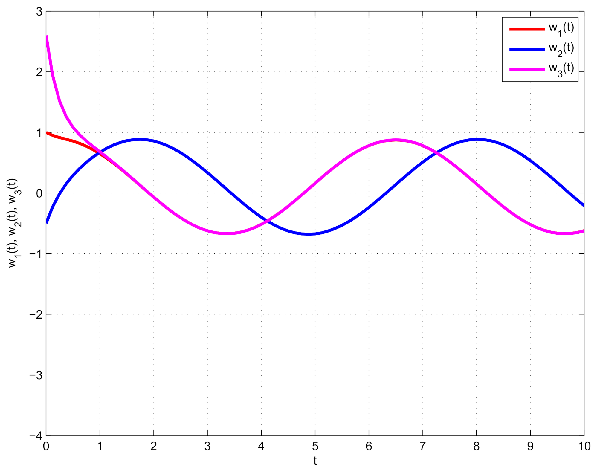
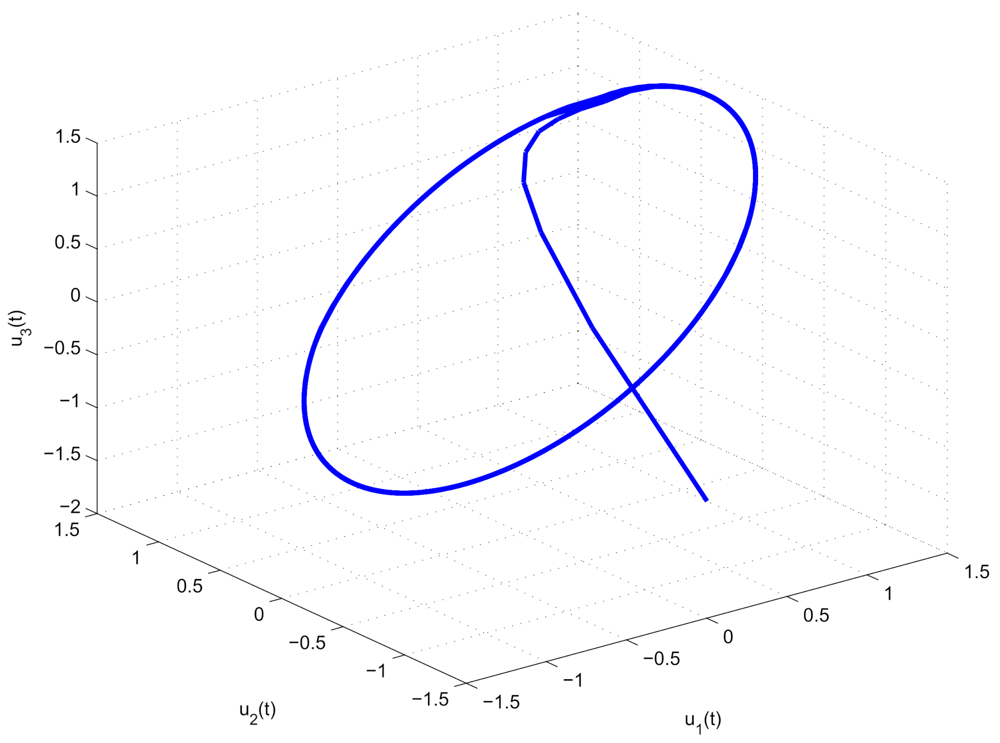
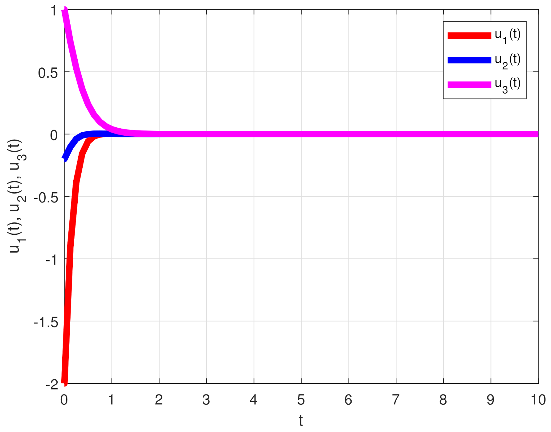
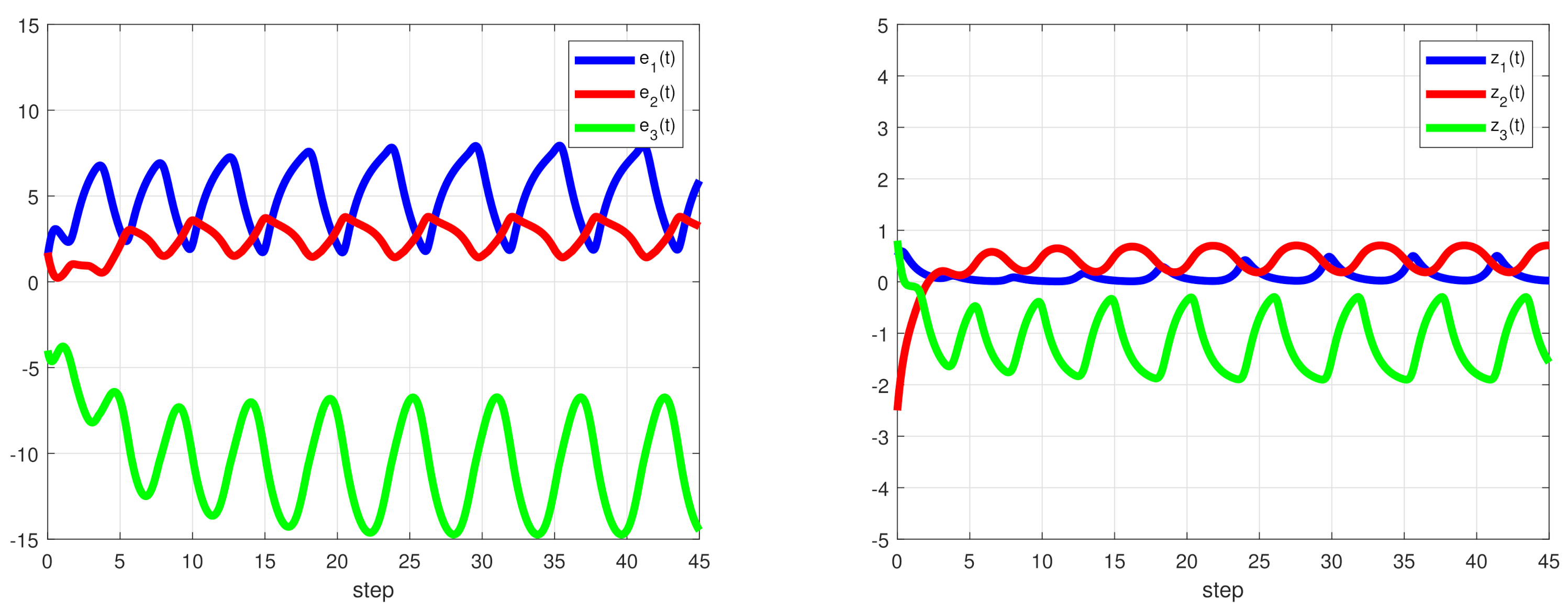
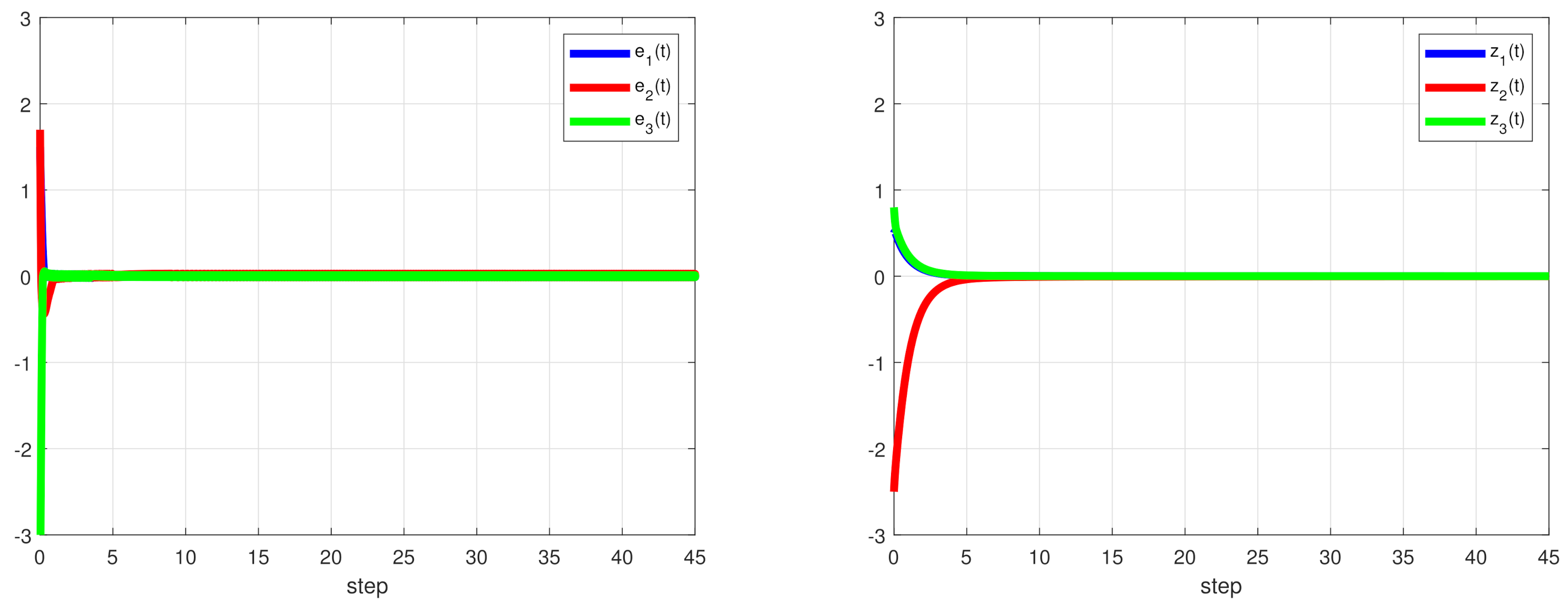
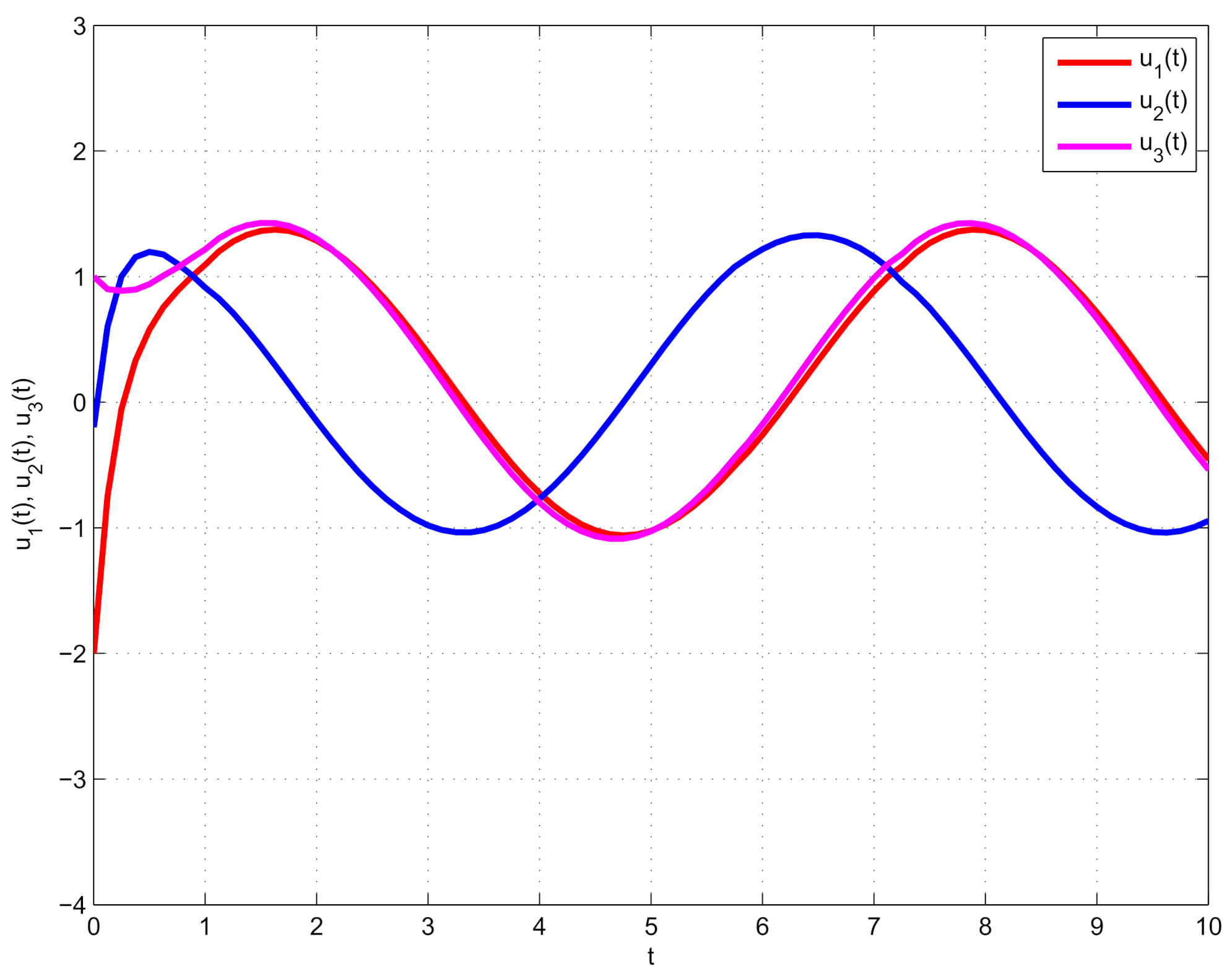
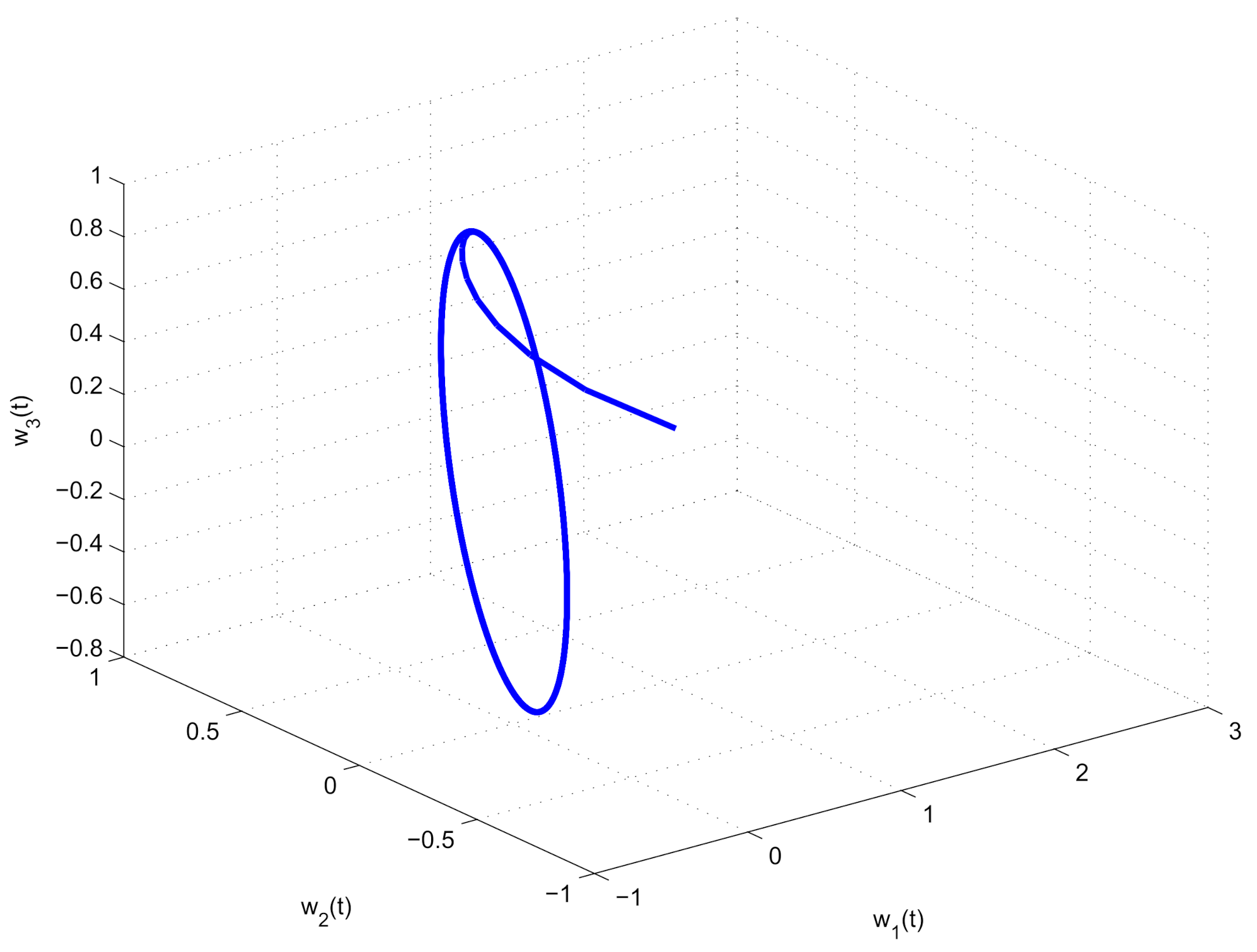
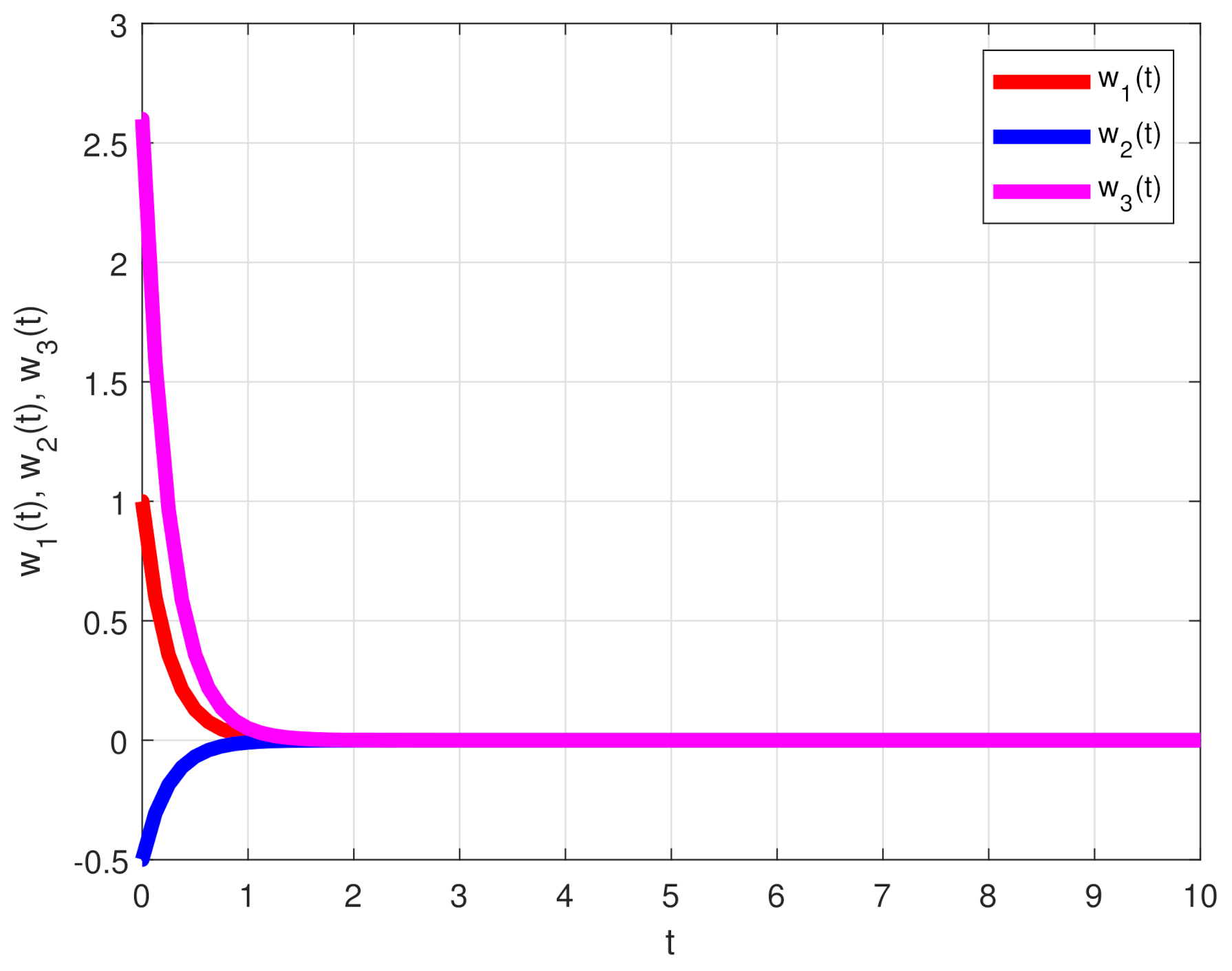
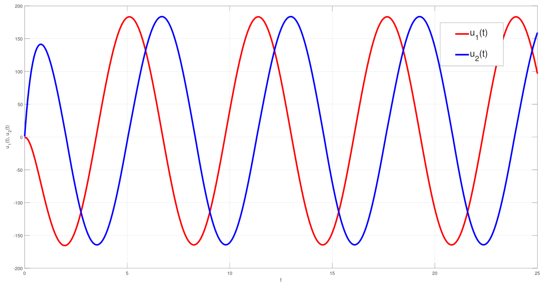
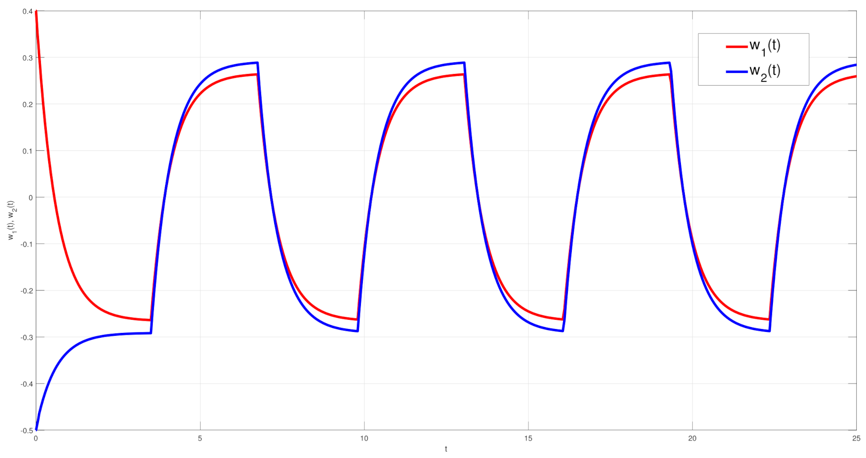
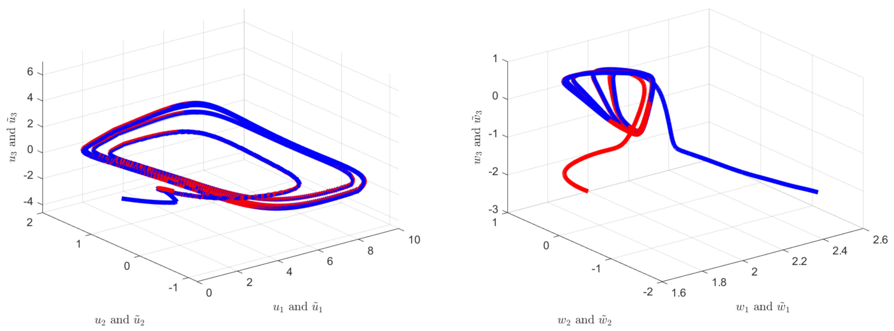
5. Numerical Results

Here, two numerical examples are given to validate the advantages of the obtained results.

Example 1.

Considering the following three-dimensional FOMBCNN:

$$\begin{array}{c}\hfill \left\{\begin{array}{c}{}_0^C{\mathcal{D}}_t^{0.98}{u}_1\left(t\right)=-4u_1\left(t\right)+q_{11}\left(u_1\left(t\right)\right)tan\left(u_1\left(t\right)\right)+q_{12}\left(u_1\left(t\right)\right)tan\left(u_2\left(t\right)\right)\hfill \\ +q_{13}\left(u_1\left(t\right)\right)tan\left(u_3\left(t\right)\right)+0.25w_1\left(t\right)+0.6(1+sint),t\ge 0\hfill \\ {}_0^C{\mathcal{D}}_t^{0.98}{u}_2\left(t\right)=-4u_2\left(t\right)+q_{21}\left(u_2\left(t\right)\right)tan\left(u_1\left(t\right)\right)+q_{22}\left(u_2\left(t\right)\right)tan\left(u_2\left(t\right)\right)\hfill \\ +q_{23}\left(u_2\left(t\right)\right)tan\left(u_3\left(t\right)\right)+0.3w_2\left(t\right)+0.6(1+cost),t\ge 0\hfill \\ {}_0^C{\mathcal{D}}_t^{0.98}{u}_3\left(t\right)=-4u_3\left(t\right)+q_{31}\left(u_3\left(t\right)\right)tan\left(u_1\left(t\right)\right)+q_{32}\left(u_3\left(t\right)\right)tan\left(u_2\left(t\right)\right)\hfill \\ +q_{33}\left(u_3\left(t\right)\right)tan\left(u_3\left(t\right)\right)+0.75w_3\left(t\right)+0.6(1+sint),t\ge 0\hfill \\ {}_0^C{\mathcal{D}}_t^{0.98}{w}_1\left(t\right)=-3w_1\left(t\right)+0.5tan\left(u_1\left(t\right)\right)+0.3(1+cost),t\ge 0\hfill \\ {}_0^C{\mathcal{D}}_t^{0.98}{w}_2\left(t\right)=-3w_2\left(t\right)+0.5tan\left(u_2\left(t\right)\right)+0.3(1+sint),t\ge 0\hfill \\ {}_0^C{\mathcal{D}}_t^{0.98}{w}_3\left(t\right)=-3w_3\left(t\right)+0.5tan\left(u_3\left(t\right)\right)+0.3(1+cost),t\ge 0,\hfill \end{array}\right.\end{array}$$

(70)

where

$$\begin{array}{ccc}\hfill q_{11}\left(u_1\left(t\right)\right)& =& \left\{\begin{array}{cc}-0.1,\hfill & |u_1\left(t\right)|\le 1\hfill \\ -0.35,\hfill & |u_1\left(t\right)|>1,\hfill \end{array}\right.q_{12}\left(u_2\left(t\right)\right)=\left\{\begin{array}{cc}0.2,\hfill & |u_2\left(t\right)|\le 1\hfill \\ 0.45,\hfill & |u_2\left(t\right)|>1,\hfill \end{array}\right.\hfill \\ \hfill q_{13}\left(u_3\left(t\right)\right)& =& \left\{\begin{array}{cc}-0.7,\hfill & |u_3\left(t\right)|\le 1\hfill \\ -0.45,\hfill & |u_3\left(t\right)|>1,\hfill \end{array}\right.q_{21}\left(u_1\left(t\right)\right)=\left\{\begin{array}{cc}0.4,\hfill & |u_1\left(t\right)|\le 1\hfill \\ 0.65,\hfill & |u_1\left(t\right)|>1,\hfill \end{array}\right.\hfill \\ \hfill q_{22}\left(u_2\left(t\right)\right)& =& \left\{\begin{array}{cc}0.35,\hfill & |u_2\left(t\right)|\le 1\hfill \\ 0.6,\hfill & |u_2\left(t\right)|>1,\hfill \end{array}\right.q_{23}\left(u_3\left(t\right)\right)=\left\{\begin{array}{cc}-0.3,\hfill & |u_3\left(t\right)|\le 1\hfill \\ -0.55,\hfill & |u_3\left(t\right)|>1,\hfill \end{array}\right.\hfill \\ \hfill q_{31}\left(u_1\left(t\right)\right)& =& \left\{\begin{array}{cc}0.20,\hfill & |u_1\left(t\right)|\le 1\hfill \\ 0.45,\hfill & |u_1\left(t\right)|>1,\hfill \end{array}\right.q_{32}\left(u_2\left(t\right)\right)=\left\{\begin{array}{cc}-0.45,\hfill & |u_2\left(t\right)|\le 1\hfill \\ -0.2,\hfill & |u_2\left(t\right)|>1,\hfill \end{array}\right.\hfill \\ \hfill q_{33}\left(u_3\left(t\right)\right)& =& \left\{\begin{array}{cc}0.50,\hfill & |u_3\left(t\right)|\le 1\hfill \\ 0.75,\hfill & |u_3\left(t\right)|>1.\hfill \end{array}\right.\hfill \end{array}$$

The measured output vector of model (71) is assumed to be:

$$\begin{array}{c}\hfill \left\{\begin{array}{c}{q}_u\left(t\right)={\mathcal{R}}_{u}u\left(t\right),\hfill \\ q_w\left(t\right)={\mathcal{R}}_{w}w\left(t\right),\hfill \end{array}\right.\end{array}$$

where

$$\begin{array}{ccc}\hfill {\mathcal{R}}_u& =& \left[\begin{array}{ccc}0.5& 0& 0\\ 0& 0.5& 0\\ 0& 0& 0.5\end{array}\right],{\mathcal{R}}_w=\left[\begin{array}{ccc}0.4& 0& 0\\ 0& 0.4& 0\\ 0& 0& 0.4\end{array}\right].\hfill \end{array}$$

We note that Assumptions $\left(\mathbf{A}\mathbf{1}\right)$ and $\left(\mathbf{A}\mathbf{2}\right)$ satisfy $\mathcal{L}=diag\{1.5,1.5,1.5\}$. By standard computation, we get

$$\begin{array}{c}\hfill \mathcal{E}=\left[\begin{array}{ccccccccc}\sqrt{0.125}& \sqrt{0.125}& \sqrt{0.125}& 0& 0& 0& 0& 0& 0\\ 0& 0& 0& \sqrt{0.125}& \sqrt{0.125}& \sqrt{0.125}& 0& 0& 0\\ 0& 0& 0& 0& 0& 0& \sqrt{0.125}& \sqrt{0.125}& \sqrt{0.125}\end{array}\right],\end{array}$$

$$\begin{array}{c}\hfill \mathcal{G}={\left[\begin{array}{ccccccccc}\sqrt{0.125}& 0& 0& \sqrt{0.125}& 0& 0& \sqrt{0.125}& 0& 0\\ 0& \sqrt{0.125}& 0& 0& \sqrt{0.125}& 0& 0& \sqrt{0.125}& 0\\ 0& 0& \sqrt{0.125}& 0& 0& \sqrt{0.125}& 0& 0& \sqrt{0.125}\end{array}\right]}^T.\end{array}$$

Let ${\sigma }_1=2,{\sigma }_2=10$, $T_{\sigma }=3$ and ${\mathcal{H}}_1={\mathcal{H}}_2=I$. Then, it is clear that the given LMIs (14) and (15) of Theorem 3 are feasible, and these solutions are given as follows:

$$\begin{array}{ccc}\hfill {\mathcal{H}}_1& =& \left[\begin{array}{ccc}8.4304& -0.0155& -0.0217\\ -0.0155& 8.4287& 0.1362\\ -0.0217& 0.1362& 8.2164\end{array}\right],{\mathcal{H}}_2=\left[\begin{array}{ccc}7.7009& 0& 0\\ 0& 7.7009& 0\\ 0& 0& 7.7009\end{array}\right],\hfill \end{array}$$

$\upsilon =50.25$, ${\alpha }_1=29.9694,{\alpha }_2=23.1027$, ${\alpha }_3=23.9755$, ${\alpha }_4=23.9755$, ${\alpha }_5=23.9755,\beta =23.9755$, $\kappa =23.9755,\rho =19.8736$. Moreover,

$$\begin{array}{ccc}\hfill 10& =& \underline{\vartheta }{\sigma }_2>\overline{\vartheta }{\sigma }_1+\frac{\alpha ({\lambda }_1+{\lambda }_2)}{\Gamma (\xi +1)}{T}_{\sigma }^{\xi }=8.43016.\hfill \end{array}$$

Therefore, FOMBCNN (1) is passive in finite time with respect to $\left(2,10,3,I,I,0.02,0.03\right)$. The initial values are selected to be $u\left(0\right)={(-2,-0.2,1)}^T$ and $w\left(0\right)={(1,-0.5,2.6)}^T$. Figure 1 and Figure 2 illustrate the time responses of the states of model (70) with $x\left(t\right)={[1+sint,1+cost,1+sint]}^T$ and $y\left(t\right)={[1+cost,1+sint,1+cost]}^T$. Figure 3 and Figure 4 show the phase trajectories of system (70) with inputs $x\left(t\right)={[1+sint,1+cost,1+sint]}^T$ and $y\left(t\right)={[1+cost,1+sint,1+cost]}^T$. The state curves of system (70) with inputs $x\left(t\right)={[0,0,0]}^T$ and $y\left(t\right)={[0,0,0]}^T$ are shown in Figure 5 and Figure 6.

Example 2.

Considering the following two-dimensional FOMBCNN:

$$\begin{array}{c}\hfill \left\{\begin{array}{c}{}_0^C{\mathcal{D}}_t^{0.98}{u}_1\left(t\right)=-2u_1\left(t\right)+0.5\ast q_{11}\left(u_1\left(t\right)\right)tan\left(u_1\left(t\right)\right)+q_{12}\left(u_1\left(t\right)\right)tan\left(u_2\left(t\right)\right)\hfill \\ +0.15w_1\left(t\right)+0.6(1+sint),t\ge 0\hfill \\ {}_0^C{\mathcal{D}}_t^{0.98}{u}_2\left(t\right)=-2u_2\left(t\right)+0.5\ast q_{21}\left(u_2\left(t\right)\right)tan\left(u_1\left(t\right)\right)+q_{22}\left(u_2\left(t\right)\right)tan\left(u_2\left(t\right)\right)\hfill \\ +0.18w_2\left(t\right)+0.6(1+cost),t\ge 0\hfill \\ {}_0^C{\mathcal{D}}_t^{0.98}{w}_1\left(t\right)=-1.5w_1\left(t\right)+1.05tan\left(u_1\left(t\right)\right),t\ge 0\hfill \\ {}_0^C{\mathcal{D}}_t^{0.98}{w}_2\left(t\right)=-1.5w_2\left(t\right)+1.15tan\left(u_2\left(t\right)\right)t\ge 0,\hfill \end{array}\right.\end{array}$$

(71)

where

$$\begin{array}{ccc}\hfill q_{11}\left(u_1\left(t\right)\right)& =& \left\{\begin{array}{cc}\frac{1}{6},\hfill & |u_1\left(t\right)|\le 1\hfill \\ -\frac{1}{6},\hfill & |u_1\left(t\right)|>1,\hfill \end{array}\right.q_{12}\left(u_2\left(t\right)\right)=\left\{\begin{array}{cc}\frac{1}{5},\hfill & |u_2\left(t\right)|\le 1\hfill \\ -\frac{1}{5},\hfill & |u_2\left(t\right)|>1,\hfill \end{array}\right.\hfill \\ \hfill q_{21}\left(u_1\left(t\right)\right)& =& \left\{\begin{array}{cc}\frac{1}{5},\hfill & |u_2\left(t\right)|\le 1\hfill \\ -\frac{1}{5},\hfill & |u_2\left(t\right)|>1,\hfill \end{array}\right.,q_{22}\left(u_2\left(t\right)\right)=\left\{\begin{array}{cc}\frac{1}{8},\hfill & |u_2\left(t\right)|\le 1\hfill \\ -\frac{1}{8},\hfill & |u_2\left(t\right)|>1.\hfill \end{array}\right.\hfill \end{array}$$

The measured output vector of model (71) is assumed to be:

$$\begin{array}{c}\hfill q_u\left(t\right)=\left[\begin{array}{cc}0.8& 0\\ 0& 1\end{array}\right]u\left(t\right),\end{array}$$

With a simple calculation, we get

$$\begin{array}{c}\hfill \mathcal{E}=\left[\begin{array}{cccc}\sqrt{0.166}& \sqrt{0.2}& 0& 0\\ 0& 0& \sqrt{0.2}& \sqrt{0.125}\end{array}\right],\mathcal{G}={\left[\begin{array}{cccc}\sqrt{0.166}& 0& \sqrt{0.2}& 0\\ 0& \sqrt{0.2}& 0& \sqrt{0.125}\end{array}\right]}^T.\end{array}$$

Then, by solving (36) and (37) of Corollary 1 with the LMI solver in MATLAB, we can get the following feasible solutions:

$$\begin{array}{ccc}\hfill {\mathcal{H}}_1& =& \left[\begin{array}{cc}7.7468& -0.0414\\ -0.0414& 7.5224\end{array}\right],{\mathcal{H}}_2=\left[\begin{array}{cc}9.1107& 0\\ 0& 8.7665\end{array}\right],\hfill \end{array}$$

$\upsilon =56.5105$, ${\alpha }_1=27.7489,{\alpha }_2=13.4079$, ${\alpha }_3=20.6206$, ${\alpha }_4=20.6206,\beta =20.6117$, and $\rho =15.2692$. Therefore, FOMBCNN (71) is passive under the initial values $u\left(0\right)={(-1,1.2)}^T$ and $w\left(0\right)={(0.4,-0.5)}^T$. Figure 7 and Figure 8 illustrate the time responses of the states of model (71) with external inputs ${[1+cos\left(2t\right),1-sin\left(2t\right)]}^T$.

When solving the sufficient conditions in Corollary 1, the minimum passive index is listed in

Table 1. Minimum passive index $\upsilon$.

Methods	[60]	Corollary 1	Improvement
$\upsilon$	60.0412	56.5105	5.8804%
The number of decision variables	$n^2+3n+16$	$n^2+3n+12$	–

.

Compared with the minimum passive index υ in [60], the effective value of the result obtained in this manuscript is increased by 5.8804%. This Table 1 demonstrates that our method provides a minimum passive index than existing works [60]. Hence, the proposed method gives fewer conservative results.

Example 3.

Considering the following three-dimensional FOMBCNN:

$$\begin{array}{c}\hfill \left\{\begin{array}{c}{}_0^C{\mathcal{D}}_t^{0.98}{u}_1\left(t\right)=-0.8u_1\left(t\right)+q_{11}\left(u_1\left(t\right)\right)tan\left(u_1\left(t\right)\right)+q_{12}\left(u_1\left(t\right)\right)tan\left(u_2\left(t\right)\right)\hfill \\ +q_{13}\left(u_1\left(t\right)\right)tan\left(u_3\left(t\right)\right)+1.2w_1\left(t\right)\hfill \\ {}_0^C{\mathcal{D}}_t^{0.98}{u}_2\left(t\right)=-0.8u_2\left(t\right)+q_{21}\left(u_2\left(t\right)\right)tan\left(u_1\left(t\right)\right)+q_{22}\left(u_2\left(t\right)\right)tan\left(u_2\left(t\right)\right)\hfill \\ +q_{23}\left(u_2\left(t\right)\right)tan\left(u_3\left(t\right)\right)+1.2w_2\left(t\right)\hfill \\ {}_0^C{\mathcal{D}}_t^{0.98}{u}_3\left(t\right)=-0.8u_3\left(t\right)+q_{31}\left(u_3\left(t\right)\right)tan\left(u_1\left(t\right)\right)+q_{32}\left(u_3\left(t\right)\right)tan\left(u_2\left(t\right)\right)\hfill \\ +q_{33}\left(u_3\left(t\right)\right)tan\left(u_3\left(t\right)\right)+1.2w_3\left(t\right)\hfill \\ {}_0^C{\mathcal{D}}_t^{0.98}{w}_1\left(t\right)=-w_1\left(t\right)+2tan\left(u_1\left(t\right)\right)\hfill \\ {}_0^C{\mathcal{D}}_t^{0.98}{w}_2\left(t\right)=-w_2\left(t\right)+0.5tan\left(u_2\left(t\right)\right)\hfill \\ {}_0^C{\mathcal{D}}_t^{0.98}{w}_3\left(t\right)=-w_3\left(t\right)+tan\left(u_3\left(t\right)\right)\hfill \end{array}\right.\end{array}$$

(72)

where

$$\begin{array}{ccc}\hfill q_{11}\left(u_1\left(t\right)\right)& =& \left\{\begin{array}{cc}0.3,\hfill & |u_1\left(t\right)|\le 1\hfill \\ 0.6,\hfill & |u_1\left(t\right)|>1,\hfill \end{array}\right.q_{12}\left(u_2\left(t\right)\right)=\left\{\begin{array}{cc}-0.25,\hfill & |u_2\left(t\right)|\le 1\hfill \\ -0.5,\hfill & |u_2\left(t\right)|>1,\hfill \end{array}\right.\hfill \\ \hfill q_{13}\left(u_3\left(t\right)\right)& =& \left\{\begin{array}{cc}-3.35,\hfill & |u_3\left(t\right)|\le 1\hfill \\ -3.65,\hfill & |u_3\left(t\right)|>1,\hfill \end{array}\right.q_{21}\left(u_1\left(t\right)\right)=\left\{\begin{array}{cc}-0.1,\hfill & |u_1\left(t\right)|\le 1\hfill \\ -0.4,\hfill & |u_1\left(t\right)|>1,\hfill \end{array}\right.\hfill \\ \hfill q_{22}\left(u_2\left(t\right)\right)& =& \left\{\begin{array}{cc}1.1,\hfill & |u_2\left(t\right)|\le 1\hfill \\ 1.4,\hfill & |u_2\left(t\right)|>1,\hfill \end{array}\right.q_{23}\left(u_3\left(t\right)\right)=\left\{\begin{array}{cc}-0.4,\hfill & |u_3\left(t\right)|\le 1\hfill \\ -0.7,\hfill & |u_3\left(t\right)|>1,\hfill \end{array}\right.\hfill \\ \hfill q_{31}\left(u_1\left(t\right)\right)& =& \left\{\begin{array}{cc}1,\hfill & |u_1\left(t\right)|\le 1\hfill \\ 1.3,\hfill & |u_1\left(t\right)|>1,\hfill \end{array}\right.q_{32}\left(u_2\left(t\right)\right)=\left\{\begin{array}{cc}-0.7,\hfill & |u_2\left(t\right)|\le 1\hfill \\ -6.7,\hfill & |u_2\left(t\right)|>1,\hfill \end{array}\right.\hfill \\ \hfill q_{33}\left(u_3\left(t\right)\right)& =& \left\{\begin{array}{cc}0.2,\hfill & |u_3\left(t\right)|\le 1\hfill \\ 0.5,\hfill & |u_3\left(t\right)|>1.\hfill \end{array}\right.\hfill \end{array}$$

The response FOMBCNN with control inputs is denoted by:

$$\begin{array}{c}\hfill \left\{\begin{array}{c}{}_0^C{\mathcal{D}}_t^{0.98}{\tilde{u}}_1\left(t\right)=-0.8{\tilde{u}}_1\left(t\right)+q_{11}\left({\tilde{u}}_1\left(t\right)\right)tan\left({\tilde{u}}_1\left(t\right)\right)+q_{12}\left({\tilde{u}}_1\left(t\right)\right)tan\left({\tilde{u}}_2\left(t\right)\right)\hfill \\ +q_{13}\left({\tilde{u}}_1\left(t\right)\right)tan\left({\tilde{u}}_3\left(t\right)\right)+1.2{\tilde{w}}_1\left(t\right)+h_{11}\left(t\right)\hfill \\ {}_0^C{\mathcal{D}}_t^{0.98}{\tilde{u}}_2\left(t\right)=-0.8{\tilde{u}}_2\left(t\right)+q_{21}\left({\tilde{u}}_2\left(t\right)\right)tan\left({\tilde{u}}_1\left(t\right)\right)+q_{22}\left({\tilde{u}}_2\left(t\right)\right)tan\left({\tilde{u}}_2\left(t\right)\right)\hfill \\ +q_{23}\left({\tilde{u}}_2\left(t\right)\right)tan\left({\tilde{u}}_3\left(t\right)\right)+1.2{\tilde{w}}_2\left(t\right)+h_{12}\left(t\right)\hfill \\ {}_0^C{\mathcal{D}}_t^{0.98}{\tilde{u}}_3\left(t\right)=-0.8{\tilde{u}}_3\left(t\right)+q_{31}\left({\tilde{u}}_3\left(t\right)\right)tan\left({\tilde{u}}_1\left(t\right)\right)+q_{32}\left({\tilde{u}}_3\left(t\right)\right)tan\left({\tilde{u}}_2\left(t\right)\right)\hfill \\ +q_{33}\left({\tilde{u}}_3\left(t\right)\right)tan\left({\tilde{u}}_3\left(t\right)\right)+1.2{\tilde{w}}_3\left(t\right)+h_{13}\left(t\right)\hfill \\ {}_0^C{\mathcal{D}}_t^{0.98}{\tilde{w}}_1\left(t\right)=-{\tilde{w}}_1\left(t\right)+2tan\left({\tilde{u}}_1\left(t\right)\right)+h_{21}\left(t\right)\hfill \\ {}_0^C{\mathcal{D}}_t^{0.98}{\tilde{w}}_2\left(t\right)=-{\tilde{w}}_2\left(t\right)+0.5tan\left({\tilde{u}}_2\left(t\right)\right)+h_{22}\left(t\right)\hfill \\ {}_0^C{\mathcal{D}}_t^{0.98}{\tilde{w}}_3\left(t\right)=-{\tilde{w}}_3\left(t\right)+tan\left({\tilde{u}}_3\left(t\right)\right)+h_{33}\left(t\right).\hfill \end{array}\right.\end{array}$$

(73)

Next, we demonstrate that the drive system (72) and controlled response system (73) achieve synchronization in finite time under the discontinuous controller (46). Let $u_1\left(0\right)=0.5$, $u_2\left(0\right)=-0.5$, $u_3\left(0\right)=1$, $w_1\left(0\right)=2$, $w_2\left(0\right)=1$, $w_3\left(0\right)=-3$, ${\tilde{u}}_1\left(0\right)=2$, ${\tilde{u}}_2\left(0\right)=1.2$, ${\tilde{u}}_3\left(0\right)=-3$, ${\tilde{w}}_1\left(0\right)=2.5$, ${\tilde{w}}_2\left(0\right)=-1.5$, ${\tilde{w}}_3\left(0\right)=0.8$, ${\lambda }_j=1.5$ and ${\mu }_j=1.2$ for $j=1,2,3$. From $Assumption( \mathbf{A}\mathbf{1})$, we have $l_1=l_2=l_3=1$ and ${\tilde{\delta }}_1={\tilde{\delta }}_2={\tilde{\delta }}_3=0.5$. In controller (46), we must choose ${\omega }_1={\omega }_2={\omega }_3=8$, ${\varpi }_1={\varpi }_2={\varpi }_3=5$, ${\vartheta }_1={\vartheta }_2={\vartheta }_3=0.5$, ${\eta }_1={\eta }_2={\eta }_3=1$ and ${\theta }_1={\theta }_2={\theta }_3=0.8$. By a simple calculation, we can obtain $2{\lambda }_j\left({\omega }_j+p_j-\frac{1}{2}{s}_j\right)-{\mu }_j{b}_j{l}_j-{\sum }_{k=1}^n\left({\lambda }_j|q^{★}{|}_{jk}{l}_j+{\lambda }_k{\left|q^{★}\right|}_{kj}{l}_k\right)>0$, $2{\mu }_j\left({\varpi }_j+a_j-\frac{1}{2}{b}_j{l}_j\right)-{\lambda }_j{s}_j>0$ and ${\vartheta }_j-{\sum }_{k=1}^n|q_{jk}^{+}-q_{jk}^{-}|{\delta }_k>0$. Therefore, FOMBCNNs (72) and (73) are synchronized in finite time based on Theorem 2, and are displayed in Figure 9, Figure 10 and Figure 11; we get an upper bound of the settling time $t\le 2.2871$. The synchronization error curves of drive–response systems without and with control inputs are displayed in Figure 9 and Figure 10. The chaotic behavior of the synchronization error curves of drive–response systems with control inputs is shown in Figure 11.

6. Conclusions

Based on a robust control method, both the passivity and synchronization criterion of FOMBCNNs were investigated in this manuscript. Through a key role of fractional order properties, finite-time stability theory and fractional-order Lyapunov functional, some novel sufficient criterion was derived to ensure the designed FOMBCNN is finite-time passive. Furthermore, a finite-time discontinuous feedback control law was designed to achieve synchronization in finite time for FOMBCNNs and we also evaluated the upper bound of the settling time. The feasibility and advantages of the obtained finite-time passivity and finite-time synchronization were illustrated in two numerical computer simulations. In the future, the global Mittag–Leffler synchronization, projective synchronization and quasi-synchronization problems will be considered for FOMBCNNs via nonfragile control [63,65], delayed impulsive control [66], quantized control [67], and quantized intermittent control [68].

References

1. Song, Q.; Yu, Q.; Zhao, Z.; Liu, Y.; Alsaadi, F.E. Boundedness and global robust stability analysis of delayed complex-valued neural networks with interval parameter uncertainties. Neural Netw. 2018, 103, 55–62. [Google Scholar] [CrossRef] [PubMed]
2. Song, Q.; Yan, H.; Zhao, Z.; Liu, Y. Global exponential stability of impulsive complex-valued neural networks with both asynchronous time-varying and continuously distributed delays. Neural Netw. 2016, 81, 1–10. [Google Scholar] [CrossRef] [PubMed]
3. Song, Q.; Wang, Z. Dynamical behaviors of fuzzy reaction-diffusion periodic cellular neural networks with variable coefficients and delays. Appl. Math. Model. 2009, 33, 3533–3545. [Google Scholar] [CrossRef]
4. Song, Q.; Zhao, Z.; Li, Y. Global exponential stability of BAM neural networks with distributed delays and reaction-diffusion terms. Phys. Lett. A 2005, 335, 213–225. [Google Scholar] [CrossRef]
5. Arbi, A.; Cao, J. Pseudo-almost periodic solution on time-space scales for a novel class of competitive neutral-type neural networks with mixed time-varying delays and leakage delays. Neural Process. Lett. 2017, 46, 719–745. [Google Scholar] [CrossRef]
6. Duan, L.; Huang, L. Global dynamics of equilibrium point for delayed competitive neural networks with different time scales and discontinuous activations. Neurocomputing 2016, 123, 318–327. [Google Scholar] [CrossRef]
7. Yang, X.; Cao, J.; Long, Y.; Rui, W. Adaptive lag synchronization for competitive neural networks with mixed delays and uncertain hybrid perturbations. IEEE Trans. Neural Netw. 2010, 21, 1656–1667. [Google Scholar] [CrossRef] [PubMed]
8. Yingchun, L.; Yang, X.; Shi, L. Finite-time synchronization for competitive neural networks with mixed delays and non-identical perturbations. Neurocomputing 2016, 185, 242–253. [Google Scholar]
9. Liu, P.; Nie, X.; Liang, J.; Cao, J. Multiple Mittag–Leffler stability of fractional-order competitive neural networks with Gaussian activation functions. Neural Netw. 2018, 108, 452–465. [Google Scholar] [CrossRef]
10. Pratap, A.; Raja, R.; Cao, J.; Rajchakit, G.; Fardoun, H.M. Stability and synchronization criteria for fractional order competitive neural networks with time delays: An asymptotic expansion of Mittag Leffler function. J. Frankl. Inst. 2019, 356, 2212–2239. [Google Scholar] [CrossRef]
11. Pratap, A.; Raja, R.; Cao, J.; Rajchakit, G.; Alsaadi, F.E. Further synchronization in finite time analysis for time-varying delayed fractional order memristive competitive neural networks with leakage delay. Neurocomputing 2018, 317, 110–126. [Google Scholar] [CrossRef]
12. Pratap, A.; Raja, R.; Agarwal, R.P.; Cao, J. Stability analysis and robust synchronization of fractional-order competitive neural networks with different time scales and impulsive perturbations. Int. J. Adapt. Control Signal Process. 2019, 33, 1635–1660. [Google Scholar] [CrossRef]
13. Zhang, H.; Ye, M.; Cao, J.; Alsaedi, A. Synchronization control of Riemann–Liouville fractional competitive network systems with time-varying delay and different time scales. Int. J. Control Autom. Syst. 2018, 16, 1404–1414. [Google Scholar] [CrossRef]
14. Chua, L.Q. Memristor-the missing circuit element. IEEE Trans. Circuit Theory 1971, 18, 507–519. [Google Scholar] [CrossRef]
15. Strukov, D.B.; Snider, G.S.; Stewart, D.R.; Williams, R.S. The missing memristor found. Nature 2008, 453, 80–83. [Google Scholar] [CrossRef]
16. Mathiyalagan, K.; Anbuvithya, R.; Sakthivel, R.; Park, J.H.; Prakash, P. Non-fragile H synchronization of memristor-based neural networks using passivity theory. Neural Netw. 2016, 74, 85–100. [Google Scholar] [CrossRef]
17. Qin, X.; Wang, C.; Li, L.; Peng, H.; Yang, Y.; Ye, L. Finite-time modified projective synchronization of memristor-based neural network with multi-links and leakage delay. Chaos Solitons Fractals 2018, 116, 302–315. [Google Scholar] [CrossRef]
18. Yang, Z.; Biao, L.; Derong, L.; Yueheng, L. Pinning synchronization of memristor-based neural networks with time-varying delays. Neural Netw. 2017, 93, 143–151. [Google Scholar] [CrossRef]
19. Zhang, Z.; Liu, X.; Zhou, D.; Lin, C.; Chen, J.; Wang, H. Finite-time stabilizability and instabilizability for complex-valued memristive neural networks with time delays. IEEE Trans. Syst. Man Cybern Syst. 2018, 48, 2371–2382. [Google Scholar] [CrossRef]
20. Guo, Z.; Wang, J.; Yan, Z. Attractivity analysis of memristor-based cellular neural networks with time-varying delays. IEEE Trans. Neural Netw. Learn. Syst. 2014, 25, 704–717. [Google Scholar] [CrossRef]
21. Podlubny, I. Fractional Differential Equations; Academic Press: San Diego, CA, USA, 1999. [Google Scholar]
22. Kim, T.; Pinkham, J. A theoretical basis for the application of fractional calculus to viscoelasticity. J. Rheol. 2000, 27, 115–198. [Google Scholar]
23. Lundstrom, B.; Higgs, M.; Spain, W. Fractional differentiation by neocortical pyramidal neurons. Nat. Neurosci. 2008, 11, 1335–1342. [Google Scholar] [CrossRef]
24. Alzabut, J.; Mohammadaliee, B.; Samei, M.E. Solutions of two fractional q–integro–differential equations under sum and integral boundary value conditions on a time scale. Adv. Differ. Equ. 2020, 2020, 304. [Google Scholar] [CrossRef]
25. Alzabut, J.; Viji, J.; Muthulakshmi, V.; Sudsutad, W. Oscillatory behavior of a type of generalized proportional fractional differential equations with forcing and damping terms. Mathematics 2020, 8, 1037. [Google Scholar] [CrossRef]
26. Alzabut, J.; Selvam, A.; Dhineshbabu, R.; Kaabar, M.K.A. The Existence, Uniqueness, and stability analysis of the discrete fractional three-point boundary value problem for the elastic beam equation. Symmetry 2021, 13, 789. [Google Scholar] [CrossRef]
27. Aadhithiyan, S.; Raja, R.; Zhu, Q.; Alzabut, J.; Niezabitowski, M.; Lim, C.P. Modified projective synchronization of distributive fractional order complex dynamic networks with model uncertainty via adaptive control. Chaos Solitons Fractals 2021, 147, 110853. [Google Scholar] [CrossRef]
28. Stephen, A.; Raja, R.; Alzabut, J.; Zhu, Q.; Niezabitowski, M.; Lim, C.P. A Lyapunov–Krasovskii functional approach to stability and linear feedback synchronization control for nonlinear multi-agent systems with mixed time delays. Math. Probl. Eng. 2021, 1–20. [Google Scholar] [CrossRef]
29. Wang, F.; Yang, T.Q.; Hu, M.F. Asymptotic stability of delayed fractional-order neural networks with impulsive effects. Neurocomputing 2015, 154, 239–244. [Google Scholar] [CrossRef]
30. Wang, F.; Yang, Y.; Xu, X.; Li, L. Global asymptotic stability of impulsive fractional-order BAM neural networks with time delay. Neural Comput. Appl. 2017, 28, 345–352. [Google Scholar] [CrossRef]
31. Wu, H.; Zhang, X.; Xue, S.; Wang, L.; Wang, Y. LMI conditions to global Mittag–Leffler stability of fractional-order neural networks with impulses. Neurocomputing 2016, 193, 148–154. [Google Scholar] [CrossRef]
32. Zhang, S.; Yu, Y.; Yu, J. LMI conditions for global stability of fractional-order neural networks. IEEE Trans. Neural Netw. Learn. Syst. 2017, 28, 2423–2433. [Google Scholar] [CrossRef] [PubMed]
33. Liu, W.; Jiang, M.; Yan, M. Stability analysis of memristor-based time-delay fractional-order neural networks. Neurocomputing 2019, 323, 117–127. [Google Scholar] [CrossRef]
34. Zheng, M.; Li, L.; Peng, H.; Xiao, J.; Yang, Y.; Zhang, Y.; Zhao, H. Finite-time stability and synchronization of memristor-based fractional-order fuzzy cellular neural networks. Commun. Nonlinear Sci. Numer. Simul. 2018, 59, 272–291. [Google Scholar] [CrossRef]
35. Ailong, A.; Zhigang, Z. Global Mittag–Leffler stabilization of fractional-order memristive neural networks. IEEE Tranctions Neural Netw. Learn. Syst. 2016, 28, 2016–2027. [Google Scholar]
36. Wenting, C.; Song, Z.; Jinyu, L.; Kaili, S. Global Mittag–Leffler stabilization of fractional-order complex-valued memristive neural networks. Appl. Math. Comput. 2018, 338, 346–362. [Google Scholar]
37. Bao, H.; Cao, J.; Kurths, J. State estimation of fractional-order delayed memristive neural networks. Nonlinear Dyn. 2014, 94, 1215–1225. [Google Scholar] [CrossRef]
38. Bao, H.; Park, J.H.; Cao, J. Non-fragile state estimation for fractional-order delayed memristive BAM neural networks. Neural Netw. 2019, 119, 190–199. [Google Scholar] [CrossRef]
39. Mathiyalagan, K.; Park, J.H.; Sakthivel, R. Novel results on robust finite-time passivity for discrete-time delayed neural networks. Neurocomputing 2016, 177, 585–593. [Google Scholar] [CrossRef]
40. Qi, W.; Gao, X.; Wang, J. Finite-time passivity and passification for stochastic time-delayed Markovian switching systems with partly known transition rates. Circuits Syst. Signal Process. 2016, 35, 3913–3934. [Google Scholar] [CrossRef]
41. Rajavel, S.; Samidurai, R.; Cao, J.; Alsaedi, A.; Ahmad, B. Finite-time non-fragile passivity control for neural networks with time-varying delay. Appl. Math. Comput. 2017, 297, 145–158. [Google Scholar] [CrossRef]
42. Song, Q.; Liang, J.; Wang, Z. Passivity analysis of discrete-time stochastic neural networks with time-varying delays. Neurocomputing 2009, 72, 1782–1788. [Google Scholar] [CrossRef]
43. Song, Q.; Zhao, Z.; Yang, J. Passivity and passification for stochastic Takagi-Sugeno fuzzy systems with mixed time-varying delays. Neurocomputing 2013, 122, 330–337. [Google Scholar] [CrossRef]
44. Song, Q.; Zhao, Z. Global dissipativity of neural networks with both variable and unbounded delays. Chaos Solitons Fractals 2005, 25, 393–401. [Google Scholar] [CrossRef]
45. Wen, S.; Zeng, Z.; Huang, T.; Chen, Y. Passivity analysis of memristor-based recurrent neural networks with time-varying delays. J. Frankl. Inst. 2013, 350, 2354–2370. [Google Scholar] [CrossRef]
46. Zhixia, D.; Zeng, Z.; Zhang, H.; Wang, L.; Liheng, W. New results on passivity of fractional-order uncertain neural networks. Neurocomputing 2019, 351, 51–59. [Google Scholar]
47. Yang, X.; Li, C.; Huang, T.; Song, Q.; Chen, X. Quasi-uniform synchronization of fractional-order memristor-based neural networks with delay. Neurocomputing 2017, 234, 205–215. [Google Scholar] [CrossRef]
48. Zhang, L.; Yang, Y. Different impulsive effects on synchronization of fractional-order memristive BAM neural networks. Nonlinear Dyn. 2018, 93, 233–250. [Google Scholar] [CrossRef]
49. Liu, X.; Ho, D.W.C.; Cao, J.; Xu, W. Discontinuous observers design for finite-time consensus of multiagent systems with external disturbances. IEEE Trans. Neural Netw. Learn. Syst. 2017, 28, 2826–2830. [Google Scholar] [CrossRef]
50. Liu, X.; Ho, D.W.C.; Song, Q.; Xu, W. Finite/Fixed-time pinning synchronization of complex networks with stochastic disturbances. IEEE Trans. Cybern. 2019, 49, 2398–2403. [Google Scholar] [CrossRef]
51. Liu, X.; Ho, D.W.C.; Xie, C. Prespecified-time cluster synchronization of complex networks via a smooth control approach. IEEE Trans. Cybern. 2020, 50, 1771–1775. [Google Scholar] [CrossRef]
52. Velmurugan, G.; Rakkiyappan, R.; Cao, J. Finite-time synchronization of fractional-order memristor-based neural networks with time delays. Neural Netw. 2016, 73, 36–46. [Google Scholar] [CrossRef]
53. Xiao, J.; Zhong, S.; Li, Y.; Xu, F. Finite-time Mittag–Leffler synchronization of fractional-order memristive BAM neural networks with time delays. Neurocomputing 2017, 219, 431–439. [Google Scholar] [CrossRef]
54. Thuan, M.V.; Huong, D.C.; Hong, D.T. New results on robust finite-time passivity for fractional-order neural networks with uncertainties. Neural Process. Lett. 2019, 50, 1065–1078. [Google Scholar] [CrossRef]
55. Filippov, A.F. Differential Equations with Discontinuous Right-Hand Sides; Kluwer: Dordrecht, The Netherlands, 1988. [Google Scholar]
56. Aubin, J.P.; Cellina, A. Differential Inclusions; Springer: Berlin, Germany, 1984. [Google Scholar]
57. Kuang, J. Applied Inequalities; Shandong Science and Technology Press: Jinan, China, 2004. [Google Scholar]
58. Singh, V. New global robust stability results for delayed cellular neural networks based on norm-bounded uncertainties. Chaos Solitons Fractals 2016, 30, 1165–1171. [Google Scholar] [CrossRef]
59. Zeng, H.B.; He, Y.; Wu, M.; Xiao, H.Q. Improved conditions for passivity of neural networks with a time-varying delay. IEEE Trans. Cybern. 2014, 44, 785–792. [Google Scholar] [CrossRef]
60. Rajchakit, G.; Chanthorn, P.; Niezabitowski, M.; Raja, R.; Baleanu, D.; Pratap, A. Impulsive effects on stability and passivity analysis of memristor-based fractional-order competitive neural networks. Neurocomputing 2020, 417, 290–301. [Google Scholar] [CrossRef]
61. Zhang, W.; Yang, X.; Yang, S.; Alsaedi, A. Finite-time and fixed-time bipartite synchronization of complex networks with signed graphs. Math. Comput. Simul. 2021, 188, 319–329. [Google Scholar] [CrossRef]
62. Zhou, Y.; Wan, X.; Huang, C.; Yang, X. Finite-time stochastic synchronization of dynamic networks with nonlinear coupling strength via quantized intermittent control. Appl. Math. Comput. 2020, 376, 125157. [Google Scholar] [CrossRef]
63. Yang, X.; Ho, D.W.C. Synchronization of delayed memristive neural networks: Robust analysis approach. IEEE Trans. Cybern. 2016, 46, 3377–3387. [Google Scholar] [CrossRef]
64. Yang, X.; Cao, J.; Liang, J. Exponential synchronization of memristive neural networks with delays: Interval matrix method. IEEE Trans. Neural Netw. Learn. Syst. 2017, 28, 1878–1888. [Google Scholar] [CrossRef]
65. Stephen, A.; Raja, R.; Alzabut, J.; Zhu, Q.; Niezabitowski, M.; Bagdasar, O. Mixed time-delayed nonlinear multi-agent dynamic systems for asymptotic stability and non-fragile synchronization criteria. Neural Process. Lett. 2021, 1–32. [Google Scholar] [CrossRef]
66. Yang, X.; Cao, J.; Qiu, J. pth moment exponential stochastic synchronization of coupled memristor-based neural networks with mixed delays via delayed impulsive control. Neural Netw. 2016, 65, 80–91. [Google Scholar] [CrossRef] [PubMed]
67. Zou, Y.; Su, H.; Tang, R.; Yang, X. Finite-time bipartite synchronization of switched competitive neural networks with time delay via quantized control. ISA Trans. 2021. [Google Scholar] [CrossRef] [PubMed]
68. Feng, Y.; Yang, X.; Song, Q.; Cao, J. Synchronization of memristive neural networks with mixed delays via quantized intermittent control. Appl. Math. Comput. 2018, 339, 874–887. [Google Scholar] [CrossRef]
Figure 1. The time responses of the states u 1 ( t ) , u 2 ( t ) and u 3 ( t ) of system (70) for the external inputs x ( t ) = [ 1 + sin t , 1 + cos t , 1 + sin t ] T in Example 1.
Fractalfract 06 00036 g001
Figure 2. The time responses of the states w 1 ( t ) , w 2 ( t ) and w 3 ( t ) of system (70) for the external inputs y ( t ) = [ 1 + cos t , 1 + sin t , 1 + cos t ] T in Example 1.
Fractalfract 06 00036 g002
Figure 3. The phase trajectories of u 1 ( t ) , u 2 ( t ) and u 3 ( t ) of system (70) for the external inputs x ( t ) = [ 1 + sin t , 1 + cos t , 1 + sin t ] T in Example 1.
Fractalfract 06 00036 g003
Figure 4. The phase trajectories of w 1 ( t ) , w 2 ( t ) and w 3 ( t ) of system (70) for the external inputs y ( t ) = [ 1 + cos t , 1 + sin t , 1 + cos t ] T in Example 1.
Fractalfract 06 00036 g004
Figure 5. The time responses of the states u 1 ( t ) , u 2 ( t ) and u 3 ( t ) of system (70) for the external inputs x ( t ) = [ 0 , 0 , 0 ] T in Example 1.
Fractalfract 06 00036 g005
Figure 6. The time responses of the states w 1 ( t ) , w 2 ( t ) and w 3 ( t ) of system (70) for the external inputs y ( t ) = [ 0 , 0 , 0 ] T in Example 1.
Fractalfract 06 00036 g006
Figure 7. The time responses of the states u 1 ( t ) and u 2 ( t ) of system (71) for the external inputs x ( t ) = [ 1 + cos ( 2 t ) , 1 sin ( 2 t ) ] T in Example 2.
Fractalfract 06 00036 g007
Figure 8. The time responses of the states w 1 ( t ) and w 2 ( t ) of system (71) for the external inputs x ( t ) = [ 1 + cos ( 2 t ) , 1 sin ( 2 t ) ] T in Example 2.
Fractalfract 06 00036 g008
Figure 9. Time behaviors of error signals e 1 ( t ) , e 2 ( t ) , e 3 ( t ) , z 1 ( t ) , z 2 ( t ) and z 3 ( t ) without control input in Example 2.
Fractalfract 06 00036 g009
Figure 10. Time behaviors of error signals e 1 ( t ) , e 2 ( t ) , e 3 ( t ) , z 1 ( t ) , z 2 ( t ) and z 3 ( t ) with control input in Example 2.
Fractalfract 06 00036 g010
Figure 11. Chaotic behaviors e 1 ( t ) , e 2 ( t ) , e 3 ( t ) , and z 1 ( t ) , z 2 ( t ) , z 3 ( t ) of systems (72) and (73) with control inputs in Example 2.
Fractalfract 06 00036 g011