A Neuro-Evolution Heuristic Using Active-Set Techniques to Solve a Novel Nonlinear Singular Prediction Differential Model

Abstract

In this study, a novel design of a second kind of nonlinear Lane–Emden prediction differential singular model (NLE-PDSM) is presented. The numerical solutions of this model were investigated via a neuro-evolution computing intelligent solver using artificial neural networks (ANNs) optimized by global and local search genetic algorithms (GAs) and the active-set method (ASM), i.e., ANN-GAASM. The novel NLE-PDSM was derived from the standard LE and the PDSM along with the details of singular points, prediction terms and shape factors. The modeling strength of ANN was implemented to create a merit function based on the second kind of NLE-PDSM using the mean squared error, and optimization was performed through the GAASM. The corroboration, validation and excellence of the ANN-GAASM for three distinct problems were established through relative studies from exact solutions on the basis of stability, convergence and robustness. Furthermore, explanations through statistical investigations confirmed the worth of the proposed scheme.

1. Introduction

The singular models arise in many applications of science, technology and engineering. One of the most important and valuable singular models is Lane–Emden (LE), which was achieved by the joint work of Lane and Emden working on the classical law of thermodynamics [1]. The LE model has many applications in astrophysics [2], mathematical physics [3], physical models [4], catalytic diffusion reactions [5], stellar configuration [6], simulated annealing [7], error estimation [8] and exothermic reactions [9]. It is always difficult to solve LE models due to a singular point at the origin, and there are few existing deterministic methods that have been implemented to solve the singular models [10,11,12,13,14]. The standard form of the second kind of LE is given as [15,16]:

$$\{\begin{array}{l}\frac{d^{2}f}{d{t}^2}+\frac{\Omega }{t}\frac{df}{dt}+g(f)=u(t),\\ f(0)=a_1,\frac{df(0)}{dt}=a_2,\end{array},$$

(1)

where $\Omega \ge 1$ is the value of the shape vector, f is dependent on t, g is some known function of dependent variable f(t), and t = 0 shows the singularity at the origin. a₁ and a₂ are the constant values.

The design of a prediction differential (PD) model is obtainable by keeping the impression of the delay differential (DD) model that was introduced by Newton and Leibnitz in the 16th century. The DD model has been implemented in extensive applications, such as transport systems, engineering fields, communication networks, population dynamics and economic studies [17,18,19,20]. Many researchers solved the DD model by considering its significance in various ways; e.g., Bildik et al. [21] applied a perturbation iteration scheme, Aziz et al. [22] used the Haar wavelet, Tomasiello [23] introduced the fuzzy transform approach, Sabir et al. [24] applied heuristic as well as swarm approaches, Erdogan et al. [25] presented a finite difference approach, and some other recent related investigations are found in references [26,27,28]. The PD model was recently introduced and its literature form is given as [29]:

$$\{\begin{array}{l}\frac{d^{2}f}{d{t}^2}=G\left(t,f(t),f(t+\lambda )\right),\hspace{0.17em}\hspace{0.17em}\hspace{0.17em}\hspace{0.17em}\lambda >0,b\le t\le c,\\ f(t)=\theta (t),\hspace{0.17em}\hspace{0.17em}\Psi \le t\le b,\hspace{0.17em}\hspace{0.17em}\hspace{0.17em}\hspace{0.17em}0\le \lambda \le \left|\Psi -b\right|,\\ \frac{df(b)}{dt}=W,\end{array}$$

(2)

where λ is the predictive factor, f(t + λ) adds some values in time that show the prediction form of function f(t), and θ(t) depicts the initial condition, while the function G is represented in terms of t, f(t) and f(t + λ). The goal of the current research is to present the design of a novel nonlinear Lane–Emden prediction differential singular model (NLE-PDSM) model of the second kind, solved numerically using artificial neural networks (ANN) optimized via the genetic algorithm (GA) and active-set method (ASM), i.e., ANN-GAASM.

The remainder of this paper is organized as follows: Section 2 presents the structure of NLE-PDSM; Section 3 presents the proposed form of the ANN-GAASM. The mathematical notations are given in Section 4. In Section 5, numerical investigations and result simulations are provided, while the conclusion is listed in the final section.

2. Construction of Second Order NLE-PDSM

The second kind of NLE-PDSM was constructed using the standard forms of the LE and PD equations described in Equations (1) and (2). The mathematical formulation of the NLE-PDSM is given as:

$$t^{-\Omega }\frac{d^l}{d{t}^l}\left(t^{\Omega }\frac{d^r}{d{t}^r}f(t+\lambda )\right)+g(f)=0,$$

(3)

where Ω is the positive number, f(t + λ) indicates the addition of values in time that show the prediction form of function f(t) and g is the function of f(t). To present the second kind of NLE-PDSM, fix the l and r values as:

$$l+r=2,\hspace{0.17em}\hspace{0.17em}\hspace{0.17em}l,r\ge 1.$$

(4)

Using the Equations (3) and (4), the obtained form is:

$$\{\begin{array}{l}\frac{d^2}{d{t}^2}f(t+\lambda )+\frac{\Omega }{t}\frac{d}{dt}f(t+\lambda )+g(f)=0,\\ f(0)=a,\frac{df(0)}{dt}=0.\end{array}$$

(5)

The single singularity arises in the above equation at point t = 0 with shape factor $\Omega$, while the prediction terms appear twice in first and second factor. Due to the singularity and predictive terms, the model in (5) is denoted the second kind of NLE-PDSM. This NLE-PDSM was numerically evaluated using ANN-GAASM. In recent years, the scientific community has solved many singular applications and fractional and biological models by using neuro-evolution and swarm heuristic approaches. Some salient features of the novel designed NLE-PDSM as well as the proposed ANN-GAASM are summarized as:

• A novel second kind of NLE-PDSM was derived through the LE fundamental system and numerical evaluated by the proposed ANN-GAASM.
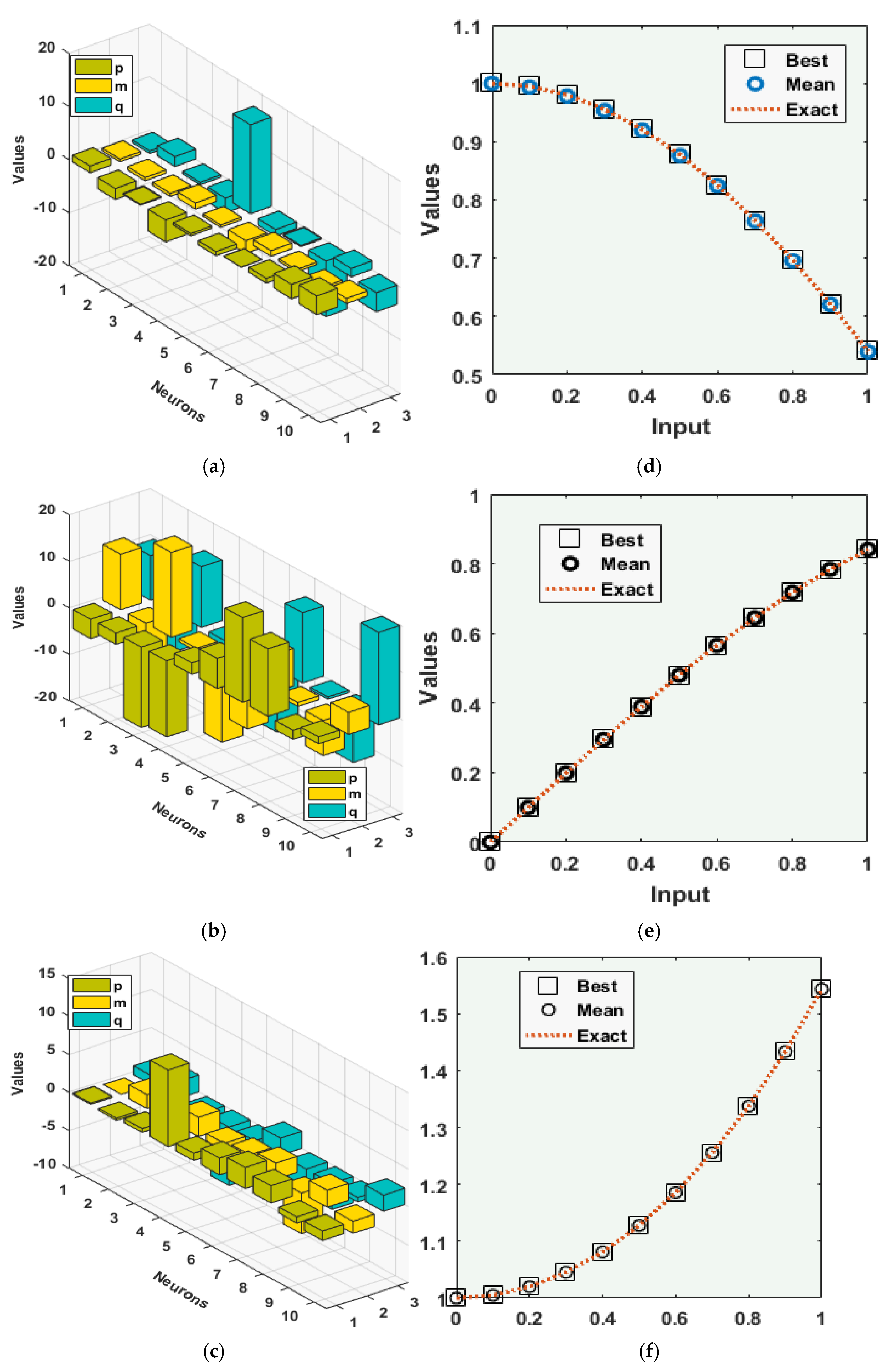
• Comparison of results using the designed model, obtained via the proposed ANN-GAASM with exact solutions, was authenticated in order to check the stability and correctness by solving three different problems using the proposed NLE-PDSM.
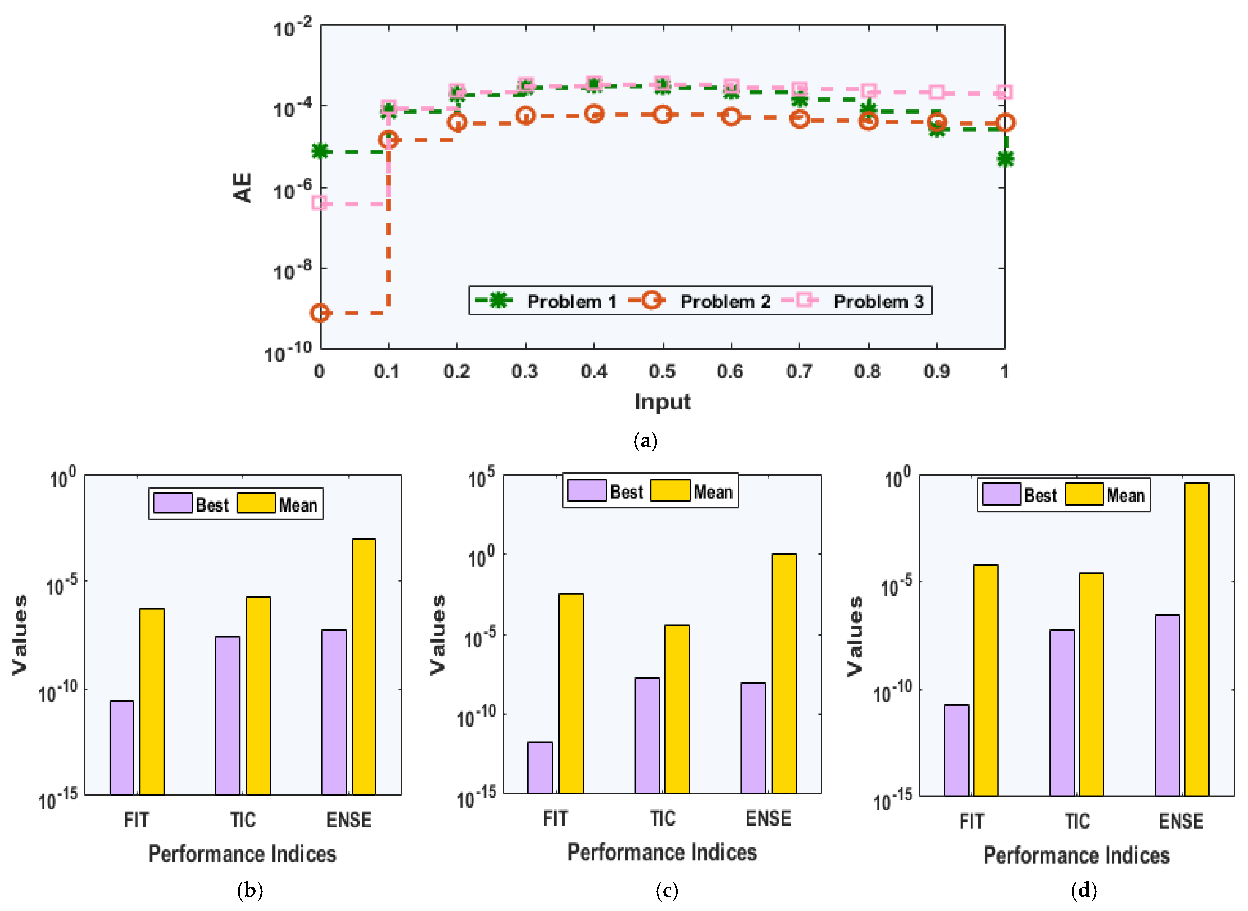
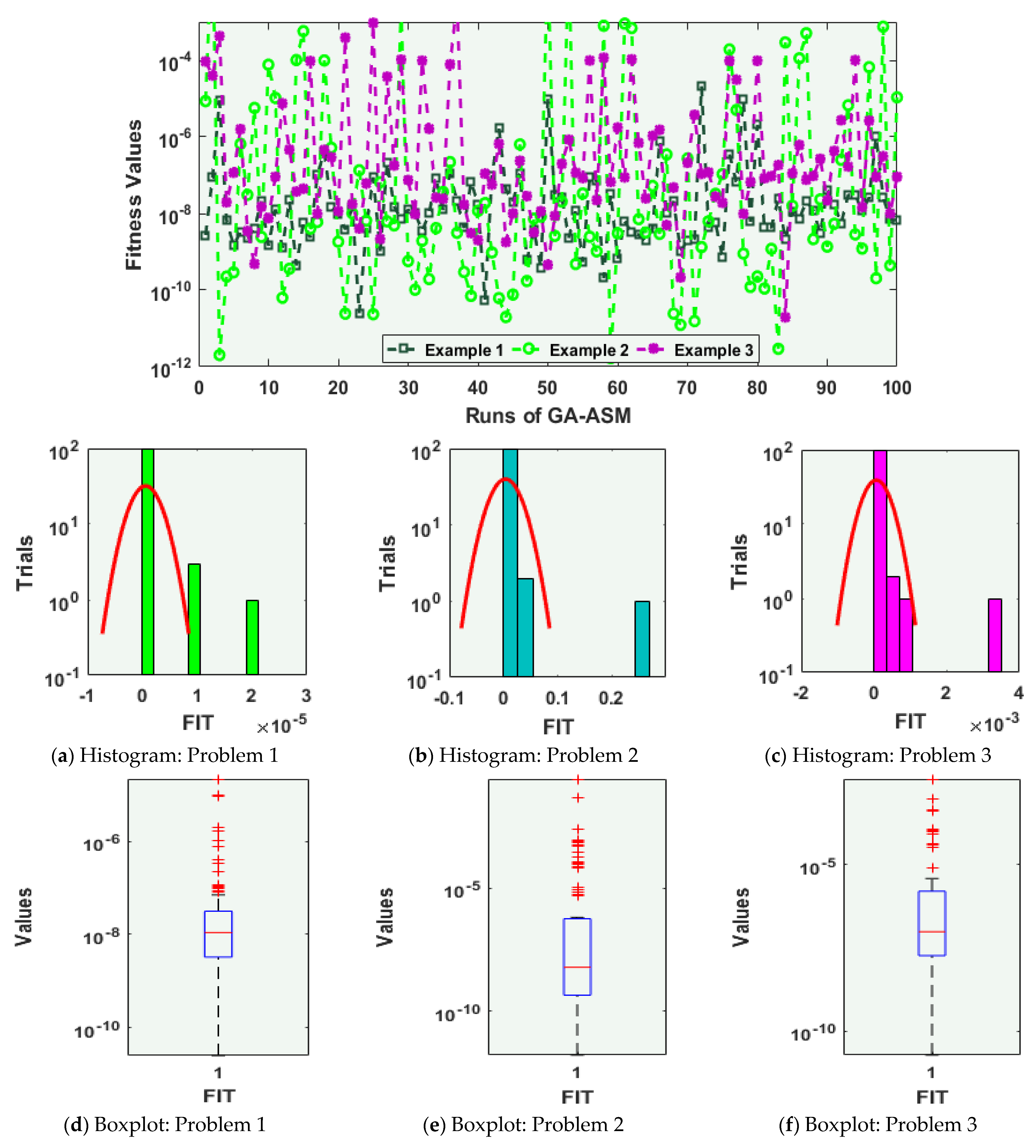
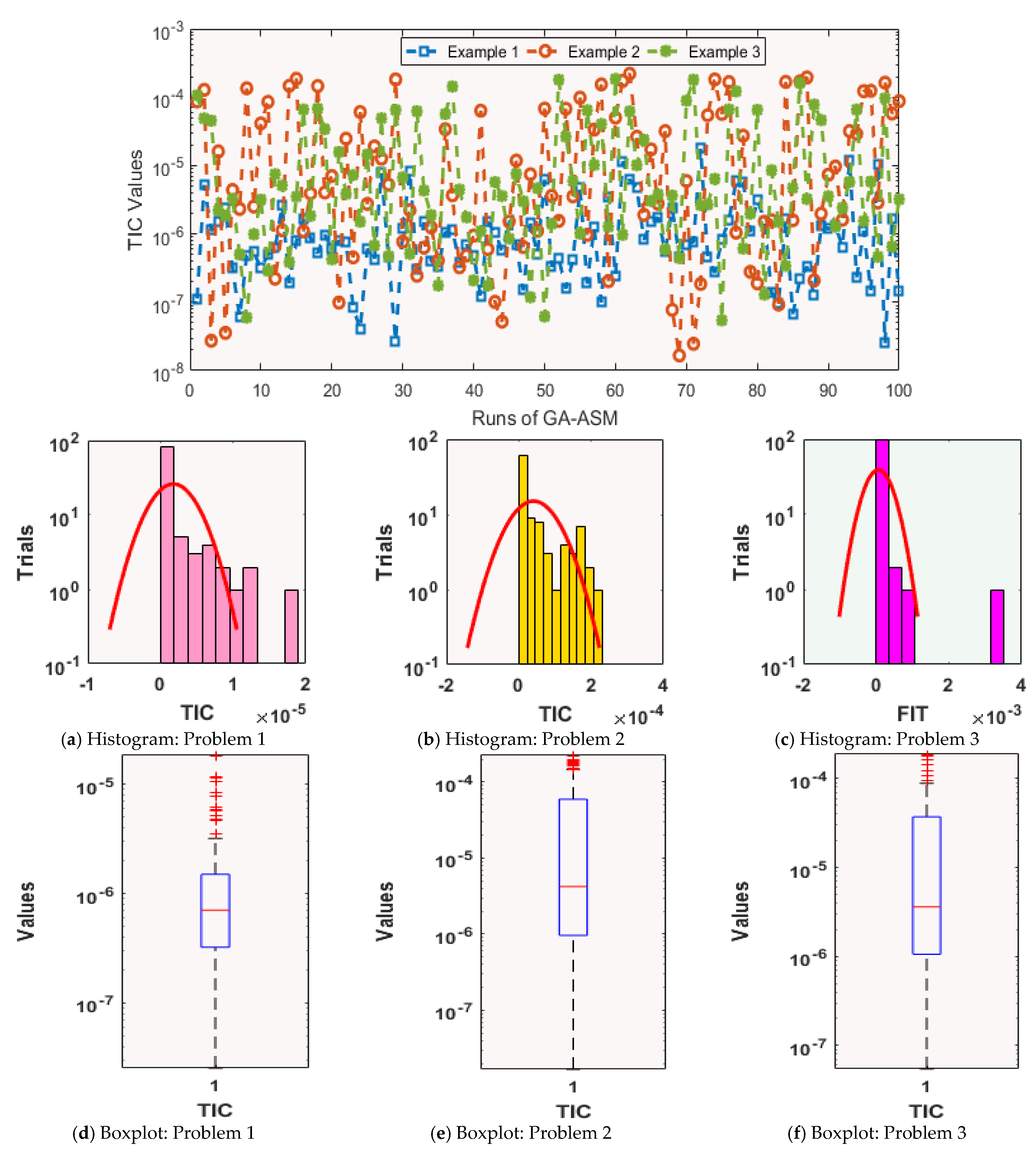
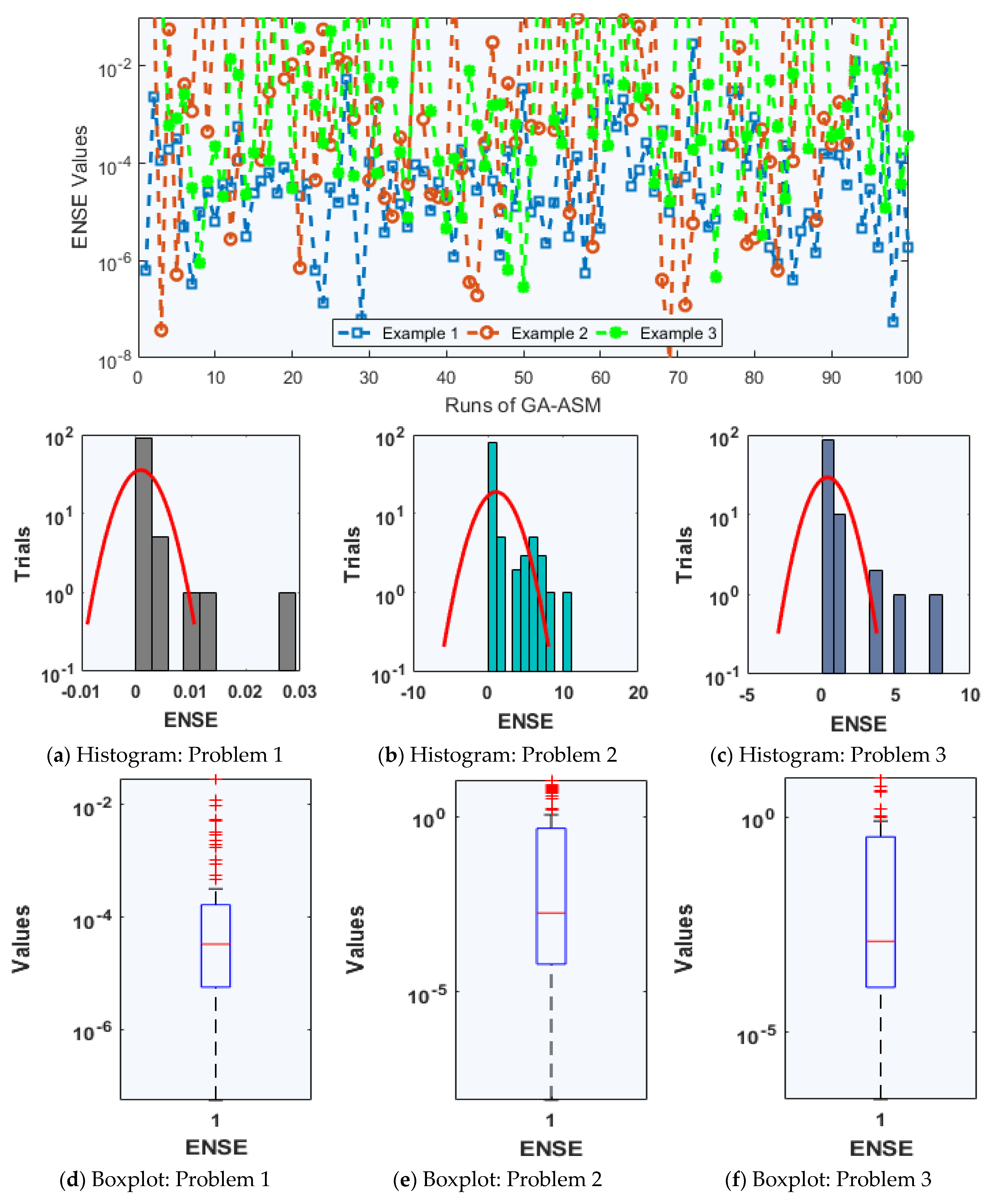
• For convergence and accuracy measurements, statistical tests based on semi interquartile range (SI-R), Nash–Sutcliffe efficiency (NSE) and Theil’s inequality coefficient (TIC) were performed to solve the second kind of NLE-PDSM.
• Alongside the reasonably precise outcomes for the NLE-PDSM, its smooth operation, stability, robustness, ease of understanding, and comprehensive applicability were other valuable compensations.

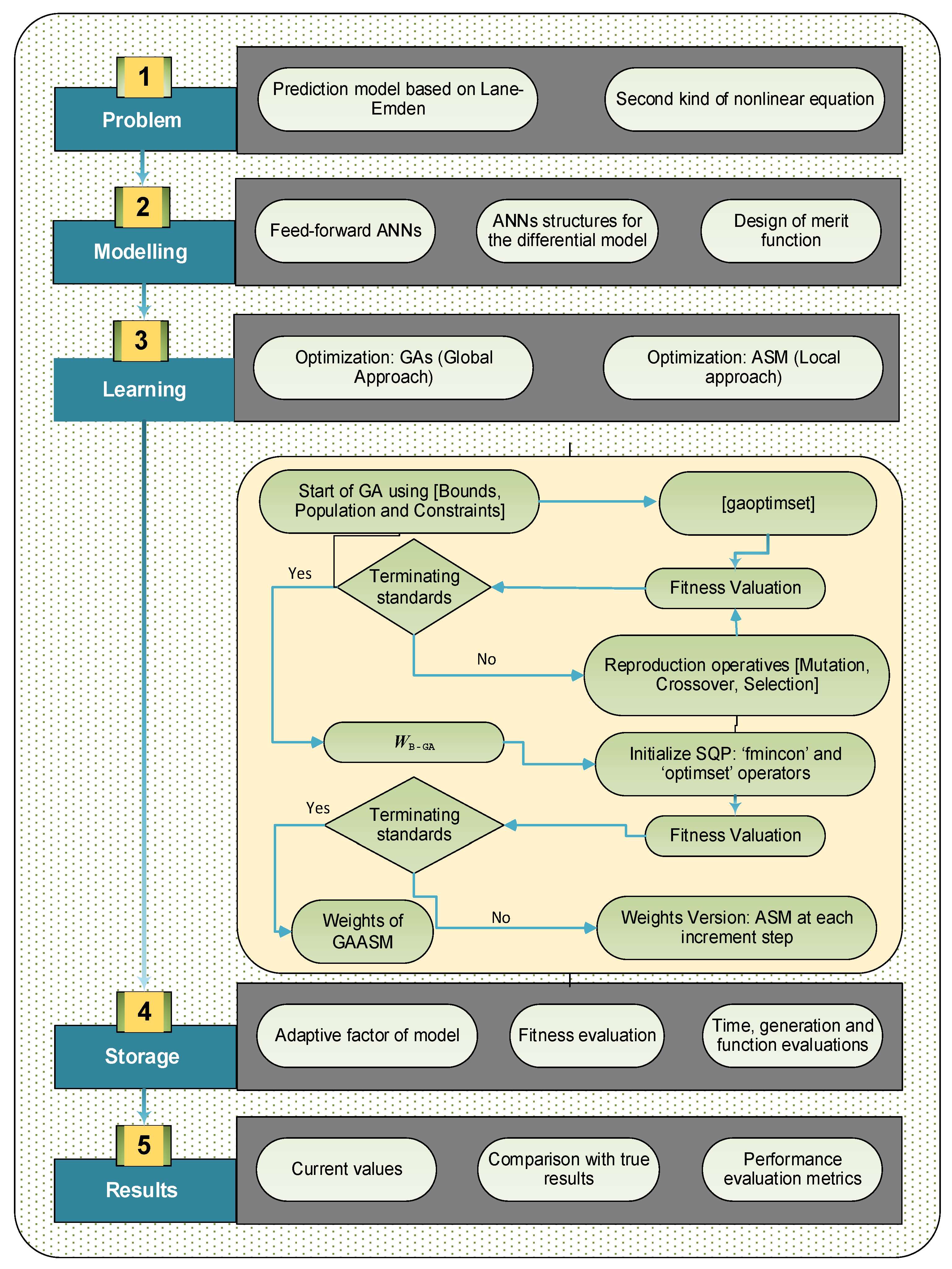
3. Solution Procedure

The suggested ANN-GAASM for solving numerical outcomes of the second kind of NLE-PDSM is categorized into two phases.

• The introduction of a merit function (MF) using the NLE-PDSM and related initial conditions;
• The provision of the optimum combination of GAASM in the form of introductory material together with pseudocode.

3.1. ANN Modeling

The mathematical systems of the NLE-PDSM were accumulated through feed-forward ANNs. $\widehat{f}(t)$ was used for the proposed results, and its derivatives using the MF, i.e., log-sigmoid $v(t)={\left(1+{\mathrm{e}}^{-t}\right)}^{-1}$, are given as:

$$\begin{array}{l}\widehat{f}(t)={\displaystyle \sum _{i=1}^k{p}_{i}v(m_{i}t+q_i)}={\displaystyle \sum _{i=1}^k\frac{p_i}{\left(1+e^{-(m_{i}t+q_i)}\right)}},\\ \frac{d\widehat{f}}{dt}={\displaystyle \sum _{i=1}^k{p}_i\frac{d}{dt}v(m_{i}t+q_i)}={\displaystyle \sum _{i=1}^k\frac{p_i{m}_i{e}^{-(m_{i}t+q_i)}}{{\left(1+e^{-(m_{i}t+q_i)}\right)}^2}},\\ \frac{d^2\widehat{f}}{d{t}^2}={\displaystyle \sum _{i=1}^k{p}_i\frac{d^2}{d{t}^2}v(m_{i}t+q_i)}={\displaystyle \sum _{i=1}^k{p}_i{m}_i^2\left(\frac{2e^{-2(m_{i}t+q_i)}}{{\left(1+e^{-(m_{i}t+q_i)}\right)}^3}-\frac{e^{-(m_{i}t+q_i)}}{{\left(1+e^{-(m_{i}t+q_i)}\right)}^2}\right)},\end{array}$$

(6)

where the weight vectors are $\mathit{p}=[p_1,p_2,p_3,\dots ,p_k],\mathit{m}=[m_1,m_2,m_3,\dots ,m_k]$ and $\mathit{q}=[q_1,q_2,q_3,\dots ,q_k]$. To solve the NLE-PDSM, a MF is given as:

$$E_{Fit}=E_{Fit-1}+E_{Fit-2},$$

(7)

where the MFs are $E_{Fit-1}$ and $E_{Fit-2}$ using the NLE-PDSM and related initial conditions, shown as:

$$E_{Fit-1}=\frac{1}{N}{\displaystyle \sum _{m=1}^N{\left(a\frac{d^2\widehat{f}(t_m+\lambda )}{d{t}_m^2}+\frac{\Omega }{t_m}\frac{d\widehat{f}(t_m+\lambda )}{d{t}_m}+g({\widehat{f}}_m)\right)}^2},$$

(8)

$$E_{Fit-2}=\frac{1}{2}{\left({\widehat{f}}_0-a\right)}^2+\frac{1}{2}{\left(\frac{d{\widehat{f}}_0}{d{t}_m}\right)}^2,$$

(9)

where ${\widehat{f}}_m=f(t_m),Nh=1,\mathrm{and}{t}_m=mh.$

3.2. Optimization Process: GAASM

The optimization of ANNs through the hybrid-computing framework of GAASM yields proficient results for solving the NLE-PDSM. Figure 1 represents the workflow diagram of the proposed ANN-GAASM for solving the second kind of NLE-PDSM.

The GA is a reliable and viable global search optimization-based approach, which is executed on unconstrained/constrained systems by applying the major metrics of reproduction with selection, mutation, elitism and crossover. It is utilized in numerous fields including information technology, applied sciences, and engineering. Some recent applications of GA include the evolutionary finite differences, evolutionary computation for nonlinear system identification, dynamics of the nonlinear Troesch’s system, pixel classification, optimal power flow for security enhancement and economic load dispatch [30,31]. These prospective applications motivated the authors to implement the GA for obtaining the decision variables of the models to solve the NLE-PDSM as shown in (5).

The ASM is a significant optimization mechanism that functions as a convex optimization scheme. It is a local search method applied to various types of constrained and unconstrained models. In recent years, ASM has been applied in various fields such as predictive control models, unconstrained minimax models and warehouse location models [32,33,34].

The laziness and slow speed of the GA can be controlled using the hybridization process of a local search ASM, i.e., a global search approach. The pseudocode of the GAASM process is provided in

Table 1. Optimization pseudocode for using the ANN-GAASM for solving the second kind of NLE-PDSM.

Global GA procedure start

i-Inputs: The designated chromosome, together with the equal ordered entries of the system, as: W = [p, m, q]

ii-Population: The chromosomes are presented as:

p = [p1, p2, p3, …, pk], m = [m1, m2, m3, …, mk] and q = [q1, q2, q3, …, qk].

iii-Output: The GA best values are labelled as

WB-GA

iv-Initialization: Design a weight vector “W” to make a chromosome. W is applied to generate P, i.e., an initial population. Fine-tune the GA values of generations.

v-Fitness scheming: Accomplish the EFit in Population for all W by using Equations (7)–(9)

vi-Termination: Terminate if any of the below conditions achieved.

EFit = 10−20, [Iterations = 85], StallLimit = 130, TolFun = 10−19, Population = 180, TolCon = 10−19, other values are defaulted

Move to storage

vii-Ranking: Rank each W in P for the EFit.

viii-Reproduction: Selection: [@selection uniform],

Mutations: @mutation adaptfeasible.

Crossover: @crossover heuristic,

Elitism: To obtain the best p values, continue the fitness assessment step.

ix- Storage: Store WB-GA, Generations, EFit, time and counts of function for existing trials of GA.

End of GA

ASM Started

i- Inputs: WB-GA is taken as start point.

ii-Output: The best GAASM weights are indicated as WGAASM.

iii- Initialize: Use WB-GA, bounded constraints, assignments, generations and other values.

iv-Terminate: Algorithm stops when any of these criteria are met.

EFit = 10−18, Iterations = 550, [TolCon = TolX = TolFun = 10−21] and [MaxFunEvals = 274,000]

While terminate

v-Calculation of fitness: Compute EFit, W, by using Equations (7)–(9)

vi- Adjustments: For the ASM, invoke “fmincon” routine. Calculate EFit of enhanced W by using Equations (7)–(9)

vii-Accumulate: Regulate WGAASM, time, EFit, generations and function counts.

ASM process End

Data Generations: The GAASM procedure repeats 100 times to find an extended data set of the optimization variables to solve the second kind of NLE-PDSM

.

4. Model Performance

The TIC, NSE and SI-R statistical operators were used together with the global operators to solve the second kind of NLE-PDSM. The mathematical notations of these operators are given as:

$$\mathrm{TIC}=\frac{\sqrt{\frac{1}{n}{{\displaystyle \sum _{i=1}^n\left(f_i-{\widehat{f}}_i\right)}}^2}}{\left(\sqrt{\frac{1}{n}{\displaystyle \sum _{i=1}^n{f}_i^2}}+\sqrt{\frac{1}{n}{\displaystyle \sum _{i=1}^n{\widehat{f}}_i^2}}\right)},$$

(10)

$$\mathrm{NSE}=\{1-\frac{{{\displaystyle \sum _{i=1}^n\left(f_i-\widehat{f}\right)}}^2}{{{\displaystyle \sum _{i=1}^n\left(f_i-{\overline{f}}_i\right)}}^2},\hspace{1em}\hspace{1em}{\overline{f}}_i=\frac{1}{n}{\displaystyle \sum _{i=1}^n{f}_i},$$

(11)

$$\mathrm{ENSE}=1-\mathrm{NSE},$$

(12)

$$\{\begin{array}{l}\mathrm{SI}\mathrm{Range}=0.5\times \left(Q_3-Q_1\right),\\ Q_3\mathrm{and}{Q}_1\mathrm{are}\mathrm{the}{3}^{rd}\&1^{st}\mathrm{quartiles}.\end{array}$$

(13)

5. Results Detail and Discussion

The detail of the numerical results for and discussions of three different problems based on the second kind of NLE-PDSM using the designed ANN-GAASM is provided in this section.

Problem 1.

Consider a second kind of NLE-PDSM with trigonometric functions given as:

$$\{\begin{array}{l}\frac{d^{2}f(t+1)}{d{t}^2}+\frac{1}{t}\frac{df(t+1)}{dt}+f^3={\cos }^{3}t-\frac{1}{t}\sin (t+1)-\cos (t+1),\\ f(0)=1,\hspace{1em}\hspace{1em}\frac{df(0)}{dt}=0.\end{array}$$

(14)

The MF of the Equation (14) is written as:

$$E_{Fit}=\frac{1}{N}{\displaystyle \sum _{i=1}^N{\left(\begin{array}{l}{t}_i\frac{d^2\widehat{f}(t_i+1)}{d{t}^2}+\frac{d\widehat{f}(t_i+1)}{dt}+t_i{\widehat{f}}^3\\ +t_i\cos (t_i+1)-t_i{\cos }^3{t}_i+\sin (t_i+1)\end{array}\right)}^2}+\frac{1}{2}\left({\left({\widehat{f}}_0-1\right)}^2+{\left(\frac{d{\widehat{f}}_0}{dt}\right)}^2\right)$$

(15)

The exact solution of Equation (15) is $\cos \left(t\right)$.

Problem 2.

Consider a second kind of NLE-PDSM with multiple trigonometric functions given as:

$$\{\begin{array}{l}\frac{d^{2}f(t+1)}{d{t}^2}+\frac{1}{t}\frac{df(t+1)}{dt}+f^3=-\sin (t+1)+\frac{1}{t}\cos (t+1)+{\sin }^{3}t,\\ f(0)=0,\hspace{1em}\hspace{1em}\frac{df(0)}{dt}=1.\end{array}$$

(16)

The MF of Equation (16) is written as:

$$\begin{array}{ll}{E}_{Fit}=& \frac{1}{N}{\displaystyle \sum _{i=1}^N{\left(\begin{array}{l}{t}_i\frac{d^2\widehat{f}(t_i+1)}{d{t}^2}+\frac{d\widehat{f}(t_i+1)}{dt}+t_i{\widehat{f}}^{-1}\\ +t_i\sin (t_i+1)-\cos (t_i+1)-t_i({\sin }^3{t}_i)\end{array}\right)}^2}\\ & +\frac{1}{2}\left({\left({\widehat{f}}_0\right)}^2+{\left(\frac{d{\widehat{f}}_0}{dt}-1\right)}^2\right)\end{array}$$

(17)

The exact solution of Equation (17) is $\sin (t)$.

Problem 3.

Consider a second kind of NLE-PDSM with hyperbolic trigonometric functions given as:

$$\{\begin{array}{l}\frac{d^{2}f(t+1)}{d{t}^2}+\frac{2}{t}\frac{df(t+1)}{dt}+f^3=\cosh (t+1)+\frac{2}{t}\sinh (t+1)+{\cosh }^{3}t,\\ f(0)=1,\hspace{1em}\hspace{1em}\frac{df(0)}{dt}=0.\end{array}$$

(18)

The MF of Equation (18) is written as:

$$E_{Fit}=\frac{1}{N}{\displaystyle \sum _{i=1}^N{\left(\begin{array}{l}{t}_i\frac{d^2\widehat{f}(t_i+1)}{d{t}^2}+2\frac{d\widehat{f}(t_i+1)}{dt}+t_i{e}^{\widehat{f}}\\ -t_i{e}^{t_i^2+1}-6\end{array}\right)}^2}+\frac{1}{2}\left({\left({\widehat{f}}_0-1\right)}^2+{\left(\frac{d{\widehat{f}}_0}{dt}\right)}^2\right)$$

(19)

The exact solution of Equation (19) is $\cosh (t)$.

The optimization of the second kind of NLE-PDSM was carried out by solving these three problems with the ANN-GAASM for fifty independent runs to assess the parameters of the systems. The best weight sets are provided to authenticate the numerical results of the second kind of NLE-PDSM given in set (6) using 10 neurons. The resulting mathematical representations of the designed second kind of NLE-PDSM take the form of:

$$\begin{array}{ll}{\widehat{f}}_{P-I}(t)=& \frac{1.2462}{1+e^{-(0.5195t-0.4927)}}-\frac{2.0599}{1+e^{-(-0.6122t+1.1873)}}-\frac{0.1672}{1+e^{-(-0.5884t-0.4693)}}\\ & -\frac{4.1094}{1+e^{-(1.1527t-2.7678)}}+\frac{0.4299}{1+e^{-(0.4704t+16.7669)}}-\frac{0.7927}{1+e^{-(-2.4017t-1.2057)}}\\ & +\frac{0.0434}{1+e^{-(1.0692t-0.2446)}}+\frac{0.9022}{1+e^{-(0.4697t-10.4579)}}+\frac{2.7240}{1+e^{-(0.9679t-3.6279)}}\\ & +\frac{3.4868}{1+e^{-(0.9679t-3.6279)}},\end{array}$$

(20)

$$\begin{array}{ll}{\widehat{f}}_{P-2}(t)=& \frac{-4.1356}{1+e^{-(11.9227t+9.5392)}}-\frac{2.3829}{1+e^{-(-8.9779t-7.9528)}}-\frac{17.1782}{1+e^{-(18.2362t+13.0871)}}\\ & -\frac{16.2736}{1+e^{-(0.6399t-1.1890)}}+\frac{2.4965}{1+e^{-(-16.5536t-13.5692)}}+\frac{6.4219}{1+e^{-(10.6676t-13.4406)}}\\ & +\frac{18.1336}{1+e^{-(8.0454t+15.0673)}}+\frac{14.4518}{1+e^{-(0.8423t-0.5010)}}-\frac{1.9949}{1+e^{-(-7.5743t-11.0638)}}\\ & +\frac{1.5269}{1+e^{-(4.6908t+19.6889)}},\end{array}$$

(21)

$$\begin{array}{ll}{\widehat{f}}_{P-3}(t)=& \frac{0.1711}{1+e^{-(0.0066t+1.1605)}}-\frac{0.2740}{1+e^{-(1.1811t+2.2318)}}+\frac{0.5136}{1+e^{-(0.6055t-1.0292)}}\\ & +\frac{10.0496}{1+e^{-(2.5368t-7.7197)}}+\frac{0.9901}{1+e^{-(0.9617t-0.8032)}}+\frac{2.1883}{1+e^{-(1.3496t+2.2103)}}\\ & +\frac{2.7897}{1+e^{-(2.0643t-4.5105)}}+\frac{2.2413}{1+e^{-(5.3506t-3.4608)}}-\frac{0.7656}{1+e^{-(2.1996t-0.5811)}}\\ & -\frac{1.2540}{1+e^{-(-1.5971t+2.1332)}},\end{array}$$

(22)

To solve Problems 1–3 based on the second kind of NLE-PDSM using ANN-GAASM, optimization was performed through repeating the GAASM hybridization scheme for 50 independent runs. Figure 2a–c represents the best ANN weight set that was implemented in (20–22) to find the proposed solutions using the designed ANN-GAASM. In Figure 2d–f, comparisons of the exact, mean and worst results obtained by the proposed ANN-GAASM for the second kind of NLE-PDSM are provided. One can see the overlapping of all the solutions, which signifies the accuracy of the proposed ANN-GAASM. Figure 3 indicates the absolute error (AE) and performance indices of ANN-GAASM solutions of Problems 1–3 based on the second kind of NLE-PDSM. The AE along with performance indices for Problems 1–3 using ANN-GAASM are presented in Figure 3a. It is observed that the AE values lay between 10⁻⁶ to 10⁻⁴ for all three problems. Performance investigations based on Fitness, ENSE and TIC operators are shown in Figure 3b–d. It is seen that the Fitness and TIC values lay at approximately 10⁻¹⁸–10⁻¹⁵ and 10⁻¹⁰–10⁻⁵, respectively, while the best ENSE operator values lay between 10⁻¹⁰–10⁻⁵ and the mean ENSE values lay in good ranges.

The convergence performances for solution of Problems 1–3 using ANN-GAASM in terms of Fitness, TIC and ENSE values, boxplots and histograms for 10 neurons are provided in Figure 4, Figure 5 and Figure 6. The Fitness performances are shown in Figure 4, Tic performances are illustrated in Figure 5 and ENSE values are plotted in Figure 6. It is shown that most of the runs for Problems 1–3 lay in the ranges 10⁻⁸–10⁻⁵, 10⁻⁷–10⁻⁵ and 10⁻⁵–10⁻², respectively. This can authenticate and prove the worth of the designed ANN-GAASM for solving Problems 1–3 for the second kind of NLE-PDSM.

Statistical data from 100 runs of ANN-GAASM on Problems 1–3, including the minimum (Min), median (Med), Mean, SI-R and STD, are provided in

Table 2. Statistical performances of ANN-GAASM solutions of Problems 1–3 based on the second kind of NLE-PDSM.

Index	Mode	Proposed Solutions of Problems 1–3 Based on the Second Kind of NLE-PDSM
		0	0.10	0.20	0.30	0.40	0.50	0.60	0.70	0.80	0.90	1.0
P-1	Min	3 × 10−9	3 × 10−6	8 × 10−5	9 × 10−5	4 × 10−5	3 × 10−6	1 × 10−4	1 × 10−4	6 × 10−5	2 × 10−5	4 × 10−6
	Med	4 × 10−7	5 × 10−4	1 × 10−3	2 × 10−3	3 × 10−3	4 × 10−3	5 × 10−3	5 × 10−3	5 × 10−3	6 × 10−3	6 × 10−3
	Mean	4 × 10−6	4 × 10−3	7 × 10−3	9 × 10−3	1 × 10−2	1 × 10−2	1 × 10−2	1 × 10−2	1 × 10−2	1 × 10−2	1 × 10−2
	SI-R	1 × 10−6	7 × 10−4	2 × 10−3	3 × 10−3	4 × 10−4	4 × 10−3	4 × 10−3	5 × 10−3	5 × 10−3	5 × 10−3	5 × 10−3
	STD	4 × 10−7	1 × 10−2	1 × 10−2	1 × 10−4	1 × 10−2	2 × 10−2	2 × 10−2	2 × 10−2	2 × 10−2	2 × 10−2	2 × 10−2
P-2	Min	3 × 10−9	3 × 10−6	8 × 10−5	9 × 10−5	4 × 10−5	3 × 10−6	1 × 10−4	1 × 10−4	6 × 10−5	2 × 10−5	4 × 10−6
	Med	4 × 10−7	5 × 10−4	1 × 10−3	2 × 10−3	3 × 10−3	4 × 10−3	5 × 10−3	5 × 10−3	5 × 10−3	6 × 10−3	6 × 10−3
	Mean	4 × 10−6	4 × 10−3	7 × 10−3	9 × 10−3	1 × 10−2	1 × 10−2	1 × 10−2	1 × 10−2	1 × 10−2	1 × 10−2	1 × 10−2
	SI-R	1 × 10−6	7 × 10−4	2 × 10−3	3 × 10−3	4 × 10−3	4 × 10−3	4 × 10−3	5 × 10−3	5 × 10−3	5 × 10−3	5 × 10−3
	STD	3 × 10−7	1 × 10−2	1 × 10−2	1 × 10−2	1 × 10−2	2 × 10−2	2 × 10−2	2 × 10−2	2 × 10−2	2 × 10−2	2 × 10−2
P-3	Min	3 × 10−9	3 × 10−6	8 × 10−5	9 × 10−5	4 × 10−5	3 × 10−6	1 × 10−4	1 × 10−4	6 × 10−5	2 × 10−5	4 × 10−6
	Med	4 × 10−7	5 × 10−4	1 × 10−3	2 × 10−3	3 × 10−3	4 × 10−3	5 × 10−3	5 × 10−3	5 × 10−3	6 × 10−3	6 × 10−3
	Mean	4 × 10−6	4 × 10−3	7 × 10−3	9 × 10−3	1 × 10−2	1 × 10−2	1 × 10−2	1 × 10−2	1 × 10−2	1 × 10−2	1 × 10−2
	SI-R	1 × 10−6	7 × 10−4	2 × 10−3	3 × 10−3	4 × 10−3	4 × 10−3	4 × 10−3	5 × 10−3	5 × 10−3	5 × 10−3	5 × 10−3
	STD	2 × 10−6	1 × 10−2	1 × 10−2	1 × 10−2	1 × 10−2	2 × 10−2	2 × 10−2	2 × 10−2	2 × 10−2	2 × 10−2	2 × 10−2

. These statistical data confirm the precision and accuracy of the projected ANN-GAASM. For Problems 1, 2 and 3, the Min values of the G.FIT, G.TIC and G. ENSE were in the ranges 10⁻⁹–10⁻⁵, 10⁻⁹–10⁻⁴ and 10⁻⁹–10⁻⁵ respectively; the Med, Mean and SI-R values clustered in the range 10⁻⁷–10⁻³, while most of the STD values were found in the range of 10⁻⁵–10⁻².

Table 3. Global statistics for the solution of Problems 1–3 based on the second kind of NLE-PDSM using ANN-GAASM.

Problem	G.FIT		G.TIC		G.ENSE
	Min	Mean	Min	Mean	Min	Mean
1	2.4879 × 10−11	1.0885 × 10−8	5.4910 × 10−7	2.3769 × 10−4	2.5247 × 10−8	7.0495 × 10−7
2	1.6761 × 10−12	6.1081 × 10−9	1.4696 × 10−8	4.0544 × 10−3	1.6678 × 10−8	4.2113 × 10−6
3	1.9434 × 10−11	9.4892 × 10−8	4.4825 × 10−7	2.7903 × 10−3	5.4468 × 10−8	3.6132 × 10−6

shows statistical data from 100 independent runs of ANN-GAASM in terms of the global performances of G.FIT, G.TIC and G. ENSE. These close-to-optimum performances on global statistical measures uphold the precision of ANN-GAASM.

6. Conclusions

The present work was the design of a novel second kind of nonlinear Lane–Emden prediction differential singular model (NLE-PDSM) based on the standard Lane–Emden form. The designed model provides the details of singular points, prediction terms and shape features. In order to find the precision and accuracy of the novel designed second kind of NLE-PDSM, three problems involving trigonometric and hyperbolic trigonometric functions represented with the second kind of prediction differential equation were designed, and numerical investigations were accomplished by combining artificial neural networks with global and local search proficiencies via the genetic algorithm and the active-set method. A neuro-evolution model integrated with the active-set method, ANN-GAASM, was presented and could solve the second kind of NLE-PDSM effectively by continuous representations-based modeling of ANNs optimized using the global potential of the GA together with the quick local search of the ASM. The achieved and reference results were compared, and the AE of the model lay within good measurements. Due to these results, one can conclude that the ANN-GAASM is efficient and precise for solving the second kind of NLE-PDSM. Furthermore, statistical data based on 50 executions to solve the second kind of MLE-PDSM, including the Min, Med, Max, SI-R, Std and Mean operators, authenticated the accurateness, robustness and trustworthiness of the ANN-GAASM, which was dignified by TIC and ENSE performances across 100 repetitions along with global performance indices for each problem based on the second kind of NLE-PDSM.

In the future, the designed ANN-GAASM could also be employed for two- and three-dimensional fluid dynamics models, information security models and biological models.

References

1. Hadian-Rasanan, A.; Rahmati, D.; Gorgin, S.; Parand, K. A single layer fractional orthogonal neural network for solving various types of Lane–Emden equation. New Astron. 2019, 75, 101307. [Google Scholar] [CrossRef]
2. Deniz, S.; Bildik, N. A new analytical technique for solving Lane-Emden type equations arising in astrophysics. Bull. Belg. Math. Soc.-Simon Stevin 2017, 24, 305–320. [Google Scholar] [CrossRef]
3. Singh, R.; Shahni, J.; Garg, H.; Garg, A. Haar wavelet collocation approach for Lane-Emden equations arising in mathematical physics and astrophysics. Eur. Phys. J. Plus 2019, 134, 548. [Google Scholar] [CrossRef]
4. Singh, R. A Modified Homotopy Perturbation Method for Nonlinear Singular Lane–Emden Equations Arising in Various Physical Models. Int. J. Appl. Comput. Math. 2019, 5, 64. [Google Scholar] [CrossRef]
5. Madduri, H.; Roul, P. A fast-converging iterative scheme for solving a system of Lane–Emden equations arising in catalytic diffusion reactions. J. Math. Chem. 2018, 57, 570–582. [Google Scholar] [CrossRef]
6. Abbas, F.; Kitanov, P.; Chimene, S.; Rehmani, A. Analytical Approach to Study the Generalized Lane-Emden Model Arises in the Study of Stellar Configuration. Appl. Math 2020, 14, 1–10. [Google Scholar]
7. Khan, N.A.; Shaikh, A. A smart amalgamation of spectral neural algorithm for nonlinear Lane-Emden equations with simulated annealing. J. Artif. Intell. Soft Comput. Res. 2017, 7, 215–224. [Google Scholar] [CrossRef] [Green Version]
8. Hao, T.-C.; Cong, F.-Z.; Shang, Y.-F. An efficient method for solving coupled Lane–Emden boundary value problems in catalytic diffusion reactions and error estimate. J. Math. Chem. 2018, 56, 2691–2706. [Google Scholar] [CrossRef]
9. Verma, A.K.; Tiwari, D. On some computational aspects of Hermite wavelets on a class of SBVPs arising in exothermic reactions. arXiv 2019, arXiv:1911.00495. [Google Scholar]
10. Sabir, Z.; Günerhan, H.; Guirao, J.L.G. On a New Model Based on Third-Order Nonlinear Multisingular Functional Differential Equations. Math. Probl. Eng. 2020, 2020, 1–9. [Google Scholar] [CrossRef] [Green Version]
11. He, J.H.; Ji, F.Y. Taylor series solution for Lane–Emden equation. J. Math. Chem. 2019, 57, 1932–1934. [Google Scholar] [CrossRef]
12. Singh, R.; Garg, H.; Guleria, V. Haar wavelet collocation method for Lane–Emden equations with Dirichlet, Neumann and Neumann–Robin boundary conditions. J. Comput. Appl. Math. 2019, 346, 150–161. [Google Scholar] [CrossRef]
13. Adel, W.; Sabir, Z. Solving a new design of nonlinear second-order Lane–Emden pantograph delay differential model via Bernoulli collocation method. Eur. Phys. J. Plus 2020, 135, 1–12. [Google Scholar] [CrossRef]
14. Asadpour, S.; Hosseinzadeh, H.; Yazdani, A. Numerical Solution of the Lane-Emden Equations with Moving Least Squares Method. Appl. Appl. Math. 2019, 14, 762–776. [Google Scholar]
15. Sabir, Z.; Wahab, H.A.; Umar, M.; Sakar, M.G.; Raja, M.A.Z. Novel design of Morlet wavelet neural network for solving second order Lane–Emden equation. Math. Comput. Simul. 2020, 172, 1–14. [Google Scholar] [CrossRef]
16. Sabir, Z.; Amin, F.; Pohl, D.; Guirao, J.L. Intelligence computing approach for solving second order system of Emden–Fowler model. J. Intell. Fuzzy Syst. 2020, 38, 7391–7406. [Google Scholar] [CrossRef]
17. Niculescu, S.I. Delay Effects on Stability: A Robust Control Approach; Springer Science & Business Media: Berlin, Germany, 2001; Volume 269. [Google Scholar]
18. Li, W.; Chen, B.G.; Meng, C.; Fang, W.; Xiao, Y.; Li, X.Y.; Hu, Z.F.; Xu, Y.X.; Tong, L.M.; Wang, H.Q.; et al. Ultrafast All-Optical Graphene Modulator. Nano Lett. 2014, 14, 955–959. [Google Scholar] [CrossRef]
19. Li, D.S.; Liu, M.Z. Exact solution properties of a multi-pantograph delay differential equation. J. Harbin Inst. Technol. 2000, 32, 1–3. [Google Scholar]
20. Kuang, Y. Delay Differential Equations: With Applications in Population Dynamics; Academic Press: Cambridge, MA, USA, 1993; Volume 191. [Google Scholar]
21. Bildik, N.; Deniz, S. A new efficient method for solving delay differential equations and a comparison with other methods. Eur. Phys. J. Plus 2017, 132, 51. [Google Scholar] [CrossRef]
22. Aziz, I.; Amin, R. Numerical solution of a class of delay differential and delay partial differential equations via Haar wavelet. Appl. Math. Model. 2016, 40, 10286–10299. [Google Scholar] [CrossRef]
23. Tomasiello, S. An alternative use of fuzzy transform with application to a class of delay differential equations. Int. J. Comput. Math. 2016, 94, 1–8. [Google Scholar] [CrossRef]
24. Sabir, Z.; Raja, M.A.Z.; Umar, M.; Shoaib, M. Neuro-swarm intelligent computing to solve the second-order singular functional differential model. Eur. Phys. J. Plus 2020, 135. [Google Scholar] [CrossRef]
25. Erdogan, F.; Sakar, M.G.; Saldır, O. A finite difference method on layer-adapted mesh for singularly perturbed delay differential equations. Appl. Math. Nonlinear Sci. 2020, 5, 425–436. [Google Scholar] [CrossRef]
26. Caraballo, T.; Diop, M.A.; Mane, A. Controllability for neutral stochastic functional integrodifferential equations with infinite delay. Appl. Math. Nonlinear Sci. 2016, 1, 493–506. [Google Scholar] [CrossRef] [Green Version]
27. Valliammal, N.; Ravichandran, C.; Park, J.H. On the controllability of fractional neutral integrodifferential delay equations with nonlocal conditions. Math. Methods Appl. Sci. 2017, 40, 5044–5055. [Google Scholar] [CrossRef]
28. Shvets, A.; Makaseyev, A. Deterministic chaos in pendulum systems with delay. Appl. Math. Nonlinear Sci. 2019, 4, 1–8. [Google Scholar] [CrossRef] [Green Version]
29. Sabir, Z.; Guirao, J.L.G.; Saeed, T.; Erdoğan, F. Design of a Novel Second-Order Prediction Differential Model Solved by Using Adams and Explicit Runge–Kutta Numerical Methods. Math. Probl. Eng. 2020, 2020, 1–7. [Google Scholar] [CrossRef]
30. Maulik, U.; Bandyopadhyay, S. Fuzzy partitioning using a real-coded variable-length genetic algorithm for pixel classification. IEEE Trans. Geosci. Remote. Sens. 2003, 41, 1075–1081. [Google Scholar] [CrossRef]
31. Devaraj, D.; Yegnanarayana, B. Genetic-algorithm-based optimal power flow for security enhancement. IEE Proc.-Gener. Transm. Distrib. 2005, 152, 899–905. [Google Scholar] [CrossRef]
32. Klaučo, M.; Kalúz, M.; Kvasnica, M. Machine learning-based warm starting of active set methods in embedded model predictive control. Eng. Appl. Artif. Intell. 2018, 77, 1–8. [Google Scholar] [CrossRef]
33. Zhou, Z.; Yang, Q. An Active Set Smoothing Method for Solving Unconstrained Minimax Problems. Math. Probl. Eng. 2020, 2020, 9108150. [Google Scholar] [CrossRef]
34. Abo-Elnaga, Y.; El-Sobky, B.; Al-Naser, L. An active-set trust-region algorithm for solving warehouse location problem. J. Taibah Univ. Sci. 2017, 11, 353–358. [Google Scholar] [CrossRef]
Figure 1. Workflow diagram of the proposed ANN-GAASM for solving the second kind of NLE-PDSM.
Fractalfract 06 00029 g001
Figure 2. ANN best weights and result comparisons using the ANN-GAASM for Problems 1 to 3 based on the second kind of NLE-PDSM. (a) ANN weights based on Problem 1. (b) ANN weights based on Problem 2. (c) ANN weights based on Problem 3. (d) Result comparison for Problem 1. (e) Result comparison for Problem 2. (f) Result comparison for Problem 3.
Fractalfract 06 00029 g002
Figure 3. AE and performance indices of ANN-GAASM solutions of Problems 1–3 based on the second kind of NLE-PDSM. (a) AE values for Problems 1–3. (b) Performance indices for Problem 1. (c) Performance indices for Problem 2. (d) Performance indices for Problem 3.
Fractalfract 06 00029 g003
Figure 4. Convergence performances for the solution of Problems 1–3 based on the second kind of NLE-PDSM using ANN-GAASM in terms of FIT values; boxplots and histograms for 10 neurons. Fitness on y-axis and independent executions on x-axis.
Fractalfract 06 00029 g004
Figure 5. Convergence performances for the solution of Problems 1–3 based on the second kind of NLE-PDSM using ANN-GAASM in terms of TIC values; boxplots and histograms for 10 neurons. TIC on y-axis and independent executions on x-axis.
Fractalfract 06 00029 g005
Figure 6. Convergence performances for the solution of Problems 1–3 based on the second kind of NLE-PDSM using ANN-GAASM in terms of ENSE values; boxplots and histograms for 10 neurons. ENSE on y-axis and independent executions on x-axis.
Fractalfract 06 00029 g006