A Comprehensive Mathematical Model for SARS-CoV-2 in Caputo Derivative

Abstract

In the present work, we study the COVID-19 infection through a new mathematical model using the Caputo derivative. The model has all the possible interactions that are responsible for the spread of disease in the community. We first formulate the model in classical differential equations and then extend it into fractional differential equations using the definition of the Caputo derivative. We explore in detail the stability results for the model of the disease-free case when ${\mathcal{R}}_0<1$. We show that the model is stable locally when ${\mathcal{R}}_0<1$. We give the result that the model is globally asymptotically stable whenever ${\mathcal{R}}_0\le 1$. Further, to estimate the model parameters, we consider the real data of the fourth wave from Pakistan and provide a reasonable fitting to the data. We estimate the basic reproduction number for the proposed data to be ${\mathcal{R}}_0=1.0779$. Moreover, using the real parameters, we present the numerical solution by first giving a reliable scheme that can numerically handle the solution of the model. In our simulation, we give the graphical results for some sensitive parameters that have a large impact on disease elimination. Our results show that taking into consideration all the possible interactions can describe COVID-19 infection.

1. Introduction

Currently, Pakistan is experiencing the fourth wave of the pandemic with infected and death cases. Presently, the number of reported cases to date is 1,278,114 and that of reported death cases is 28,566, while the number of recovered as of 10 November 2021 is 1,226,590. The total death reported is 2% of the infected cases and the peak of infected cases suggests a third wave in the country of Pakistan. The number of active cases for the beginning of the fourth wave started in July and will hopefully end soon. The number of infected cases is decreasing daily, while the number of recoveries is increasing with a decreased number of deaths [1]. Due to the decreasing number of cases in the fourth wave, life in the country is coming back to normal. One of the reasons is that the vaccinations and the government’s strict polices made it possible to get things back to normal.

Since the beginning of the COVID-19 pandemic, many researchers in their respective fields have been studying the infection of coronavirus and trying to identify the possible ways of immunizing the human being from this virus in order to follow the rules and regulations given by the World Health Organization (WHO), and to maximally immunize individuals. Regarding the studying of the coronavirus infection from different perspectives by the researchers, it is noteworthy that mathematical models are considered effective in order to study the number of infected cases and determine the possible peak of curve and its prediction for the infected COVID-19 data. The information of finding the peak of infection in a particular country can lead to decisions on how these cases can be minimized and to minimize the occurrence of future outbreak with fewer infected cases. Some mathematical studies were designed for the understanding of coronavirus infection with the reported cases from their specific countries with different strategies of controls. The study on the COVID-19 pandemic and its modeling and forecasting in India was studied in [2]. A mathematical model was constructed for the infection outbreak in Italy and France, considering real cases [3]. Considering a case study of Pakistan to built a mathematical model with the analysis of control strategies was considered in [4]. The authors used the infected cases of Nigeria and studied the dynamics of coronavirus model in [5]. The infected cases in China and their mathematical modeling with analysis were explored in [6]. The authors in [7] considered the mathematical modeling theory to investigate the COVID-19 infection using Ethiopian cases. The authors in [8] used the approach of graph modeling to understand the COVID-19 infection. A model formulated to study the cases in India was explored in [9]. The cost effective analysis of the COVID-19 infection by utilizing the theory of an optimal control was discussed in [10]. The literature on COVID-19 dynamics is expansive as there are many works; we refer the readers to see more related work using the references in the above-mentioned studies.

Recently, researchers from different fields of science and engineering showed their interest in using fractional differential equations (FDEs) for their proposed models. An especially great interest was given to mathematical modeling in epidemiological models. Due to the many properties of FDEs, the memory effect is one of the interesting properties of fractional order models that cannot be observed in classical differential equations; see, for more details, [11]. Note that fractional calculus has become one of the most studied fields used to explain physical properties of real-world problems, such as the COVID-19 pandemic, SIR, and health problems [12,13]. Fractional differential equations in the current era are used by various researchers to model their problems. Among these research problems, the COVID-19 pandemic has been studied widely, obtaining useful results regarding the infection. For example, a fractional COVID-19 model by using the power law was considered in [14]. The COVID-19 transmission dynamics using the fractional order model was explored in [15]. A SIR model in [16] was formulated by the authors with the help of the Mittag–Leffler law. The spread of coronavirus and its mathematical modeling in Turkey and Africa with theory and applications were discussed in [17]. A fractional order model in [18] was used to study the COVID-19 infection cases in Saudi Arabia. Modeling and numerical analysis of the COVID-19 infection was explored in [19]. A mathematical model of COVID-19 with immune response and its fractional optimal control was suggested in [20].

In the present paper, we aim to study the coronavirus infection through a novel mathematical model by assuming four different contacts that are responsible for the COVID-19 infection. Among these contacts, the exposed, asymptomatic, symptomatic and the hospitalized individuals contact healthy people to spread the infection. In order to motivate the readers, it is possible that the infection is spreading through the contact of asymptomatic, symptomatic, and those hospitalized infected individuals, while the individuals that become exposed after contacting infected people can infect others during their exposed period. So, all the possible interactions are meaningful and valid, biologically. First, we give, in detail, the modeling of the coronavirus using classical differential equations and later extend it to the fractional order system using the power law (Caputo derivative). The rest of the results in the paper are split section-wise as follows: In Section 2, we discuss in detail the mathematical modeling of the COVID-19 model in integers and then extend it to the fractional order model. In Section 3, we explore the mathematical analysis of the model and its stability. We estimate the parameters of the model using the reported cases in Section 4. The numerical results and discussion on the fractional order model are discussed in Section 5. Finally, we summarize our work by the conclusion.

2. Model Formulation

To study the COVID-19 dynamics thorough a mathematical model, we denoted the population of humans by $N\left(t\right)$ at any time t and divided it further into six different sub-classes—namely, healthy or susceptible individuals $S\left(t\right)$ (the individuals that are at risk of acquiring the infection, but not yet contracted the disease); exposed individuals (the individuals infected who are incubating the infection) $E\left(t\right)$; asymptomatic individuals (individuals that do not show clinical symptoms, but are able to transmit the infection), $A\left(t\right)$; symptomatic or infected individuals (individuals that show full symptoms of disease and infect other individuals), $I\left(t\right)$; hospitalization of infected individuals (the individuals that are infected or hospitalized) $H\left(t\right)$; recovered individuals (individuals who either recovered or were removed from the population ) $R\left(t\right)$; so, $N\left(t\right)=S\left(t\right)+E\left(t\right)+A\left(t\right)+I\left(t\right)+H\left(t\right)+R\left(t\right)$. A study shows that about 80% of the individuals infected by COVID-19 are due to the asymptomatic infected individuals that do not show any symptoms [21]. In other words, the individuals in class $A\left(t\right)$ produce a lot of infected cases of COVID-19 in the population who are unaware of their infection. Due to there being no clinical symptoms of the disease in the individuals in compartment $A\left(t\right)$, disease control is more difficult. If not isolated rapidly, the individuals that show symptoms clinically detected through random diagnosed testing or the contract tracing of the confirmed COVID-19 cases will continue to unknowingly be spreading the infection. The exposed individuals who are incubating the infection also risk spreading the infection further in populations. Asymptomatic and exposed individuals in contact with healthy individuals are considered to be one of the biggest causes of COIVD-19 disease transmissions. COVID-19 with the suggested classes above and the important features of exposed and asymptomatic infection can be described in the following through evolutionary differential equations:

$$\begin{array}{ccc}\hfill \frac{dS\left(t\right)}{dt}& =& \mathrm{\Lambda }-\frac{({\beta }_{1}E\left(t\right)+{\beta }_{2}A\left(t\right)+{\beta }_{3}I\left(t\right)+{\beta }_{4}H\left(t\right))}{N\left(t\right)}S\left(t\right)-\mu S\left(t\right),\hfill \\ \hfill \frac{dE\left(t\right)}{dt}& =& \frac{({\beta }_{1}E\left(t\right)+{\beta }_{2}A\left(t\right)+{\beta }_{3}I\left(t\right)+{\beta }_{4}H\left(t\right))}{N\left(t\right)}S\left(t\right)-(\eta +\mu )E\left(t\right),\hfill \\ \hfill \frac{dA\left(t\right)}{dt}& =& \eta \nu E\left(t\right)-(q_1+\mu )A\left(t\right),\hfill \\ \hfill \frac{dI\left(t\right)}{dt}& =& (1-\nu )\eta E\left(t\right)-(q_2+\kappa +\psi +\mu )I\left(t\right),\hfill \\ \hfill \frac{dH\left(t\right)}{dt}& =& \kappa I\left(t\right)-(\omega +q_3+\mu )H\left(t\right),\hfill \\ \hfill \frac{dR\left(t\right)}{dt}& =& q_{1}A\left(t\right)+q_{2}I\left(t\right)+q_{3}H\left(t\right)-\mu R\left(t\right),\hfill \end{array}$$

(1)

subject to the non-negative conditions

$$\begin{array}{ccc}\hfill S\left(0\right)& =& S_0\ge 0, E\left(0\right)=E_0\ge 0, A\left(0\right)=A_0\ge 0, I\left(0\right)=I_0\ge 0,\hfill \\ \hfill H\left(0\right)& =& H_0\ge 0, R\left(0\right)=R_0\ge 0.\hfill \end{array}$$

(2)

In system (1), we define in detail the parameter involved. The individuals that increase the population of susceptible individuals are shown by $\mathrm{\Lambda }$, while the natural death rate of humans in each compartment is given by $\mu$ decreasing the population. The contact rates such as ${\beta }_i$ for $i=1,2\dots ,4$ represente, respectively, the contact among healthy and susceptible people, the contact among healthy people and those infected with no clinical symptoms, the contact among healthy people and those infected with clinical symptoms, the contact between healthy people and hospitalized infected people. It is assumed further that ${\beta }_1\ne {\beta }_2\ne {\beta }_3\ne {\beta }_4$. The exposed individuals progress out of the compartment E through the rate given by $\eta$, and it is assumed that a proportion $\nu \in (0,1]$ of individuals in the exposed class with no clinical symptoms move into the class (A) after the completion of the incubation period, while the proportion $1-\nu$ remaining show clinical symptoms by moving to the symptomatic infected class I through coming out of the incubation period. The parameters $q_i$ for $i=1,2,3$ denote, respectively, the recovery of asymptomatic, symptomatic and hospitalized infected people. The symptomatic individuals can be hospitalized at a rate of $\kappa$ (they can be isolated at hospital or at home). The people infected with COVID-19 die due to disease in the classes I and H are shown, respectively, by the parameters $\psi$ and $\omega$. One can estimate the total death cases reported from the model above by considering the equation $\frac{dD}{dt}=\psi I+\omega H$.

A Fractional-Order Model

Before we construct the fractional-order model, we first defined the Caputo derivative and the related results that will be required in the onward analysis. The following have been taken from [22,23].

Definition 1.

The Caputo derivative is defined through the following,

$${}^C{D}^{\varpi }g\left(t\right)=\frac{1}{\mathrm{\Gamma }(1-\varpi )}{\int }_0^t{(t-u)}^{-\varpi }{g}^{\prime }\left(u\right)du,$$

(3)

where the symbol $\mathrm{\Gamma }(1-\varpi )$ denotes Euler Gamma function, and $\varpi \in (0,1)$.

Lemma 1.

Given that the function $g\left(t\right)$ and ${}^C{D}^{\varpi }g\left(t\right)$ are both continuous on $[0,b].$, then

$$g\left(t\right)=g\left(0\right)+\frac{1}{\mathrm{\Gamma }\left(\varpi \right)}{}^C{D}^{\varpi }g\left(\zeta \right)t^{\varpi },\hspace{1em}0<\zeta <t, forevery t\in [0,b].$$

We obtain this if ${}^C{D}^{\varpi }g\left(t\right)>0$ for every $0\le t\le b$, so the function g is strictly increasing, and if ${}^C{D}^{\varpi }g\left(t\right)<0$ for every $0\le t\le b$, then g is decreasing. By extending the model (1) by following the Caputo derivative definition, we obtain the following:

$$\begin{array}{ccc}\hfill {}_0^C{D}_t^{\varpi }S\left(t\right)& =& \mathrm{\Lambda }-\lambda \left(t\right)S\left(t\right)-\mu S\left(t\right),\hfill \\ \hfill {}_0^C{D}_t^{\varpi }E\left(t\right)& =& \lambda \left(t\right)S\left(t\right)-(\eta +\mu )E\left(t\right),\hfill \\ \hfill {}_0^C{D}_t^{\varpi }A\left(t\right)& =& \eta \nu E\left(t\right)-(q_1+\mu )A\left(t\right),\hfill \\ \hfill {}_0^C{D}_t^{\varpi }I\left(t\right)& =& (1-\nu )\eta E\left(t\right)-(q_2+\kappa +\psi +\mu )I\left(t\right),\hfill \\ \hfill {}_0^C{D}_t^{\varpi }H\left(t\right)& =& \kappa I\left(t\right)-(\omega +q_3+\mu )H\left(t\right),\hfill \\ \hfill {}_0^C{D}_t^{\varpi }R\left(t\right)& =& q_{1}A\left(t\right)+q_{2}I\left(t\right)+q_{3}H\left(t\right)-\mu R\left(t\right),\hfill \end{array}$$

(4)

where

$$\begin{array}{c}\hfill \lambda \left(t\right)=\frac{({\beta }_{1}E\left(t\right)+{\beta }_{2}A\left(t\right)+{\beta }_{3}I\left(t\right)+{\beta }_{4}H\left(t\right))}{N\left(t\right)},\end{array}$$

and using the initial values of (2).

The total dynamics of the fractional-order model (4) can be obtained by adding all their equations, and it is given by

$$\begin{array}{ccc}\hfill \frac{dN}{dt}& =& \mathrm{\Lambda }-\mu N-\psi I-\omega H\le \mathrm{\Lambda }-\mu N,\hfill \end{array}$$

when $t\to \infty$

$$\begin{array}{c}\hfill \underset{t\to \infty }{lim}N\left(t\right)\le \frac{\mathrm{\Lambda }}{\mu }.\end{array}$$

The following feasible region is given for model (4), where the solutions related to the model lie in

$$\Theta =\left\{(S,E,A,I,H,R)\in {\mathbb{R}}_{+}^6:S+E+A+I+H+R⩽\frac{\mathrm{\Lambda }}{\mu }\right\}$$

(5)

3. Equilibria and Its Stability

Here, we obtain the equilibria of the fractional-order model (4) by equating the time rate of change of the system (4) to zero, and obtain the disease-free equilibrium denoted by $P_0$,

$$\begin{array}{c}\hfill P_0=\left(S_0,E_0,A_0,I_0,H_0,R_0\right)=\left(\frac{\mathrm{\Lambda }}{\mu },0,0,0,0,0\right).\end{array}$$

(6)

We next compute the basic reproduction number denoted by ${\mathcal{R}}_0$, which is defined as: the average secondary infection introduced into a population of purely susceptible individuals producing further secondary infection. The expression for the basic reproduction number can be obtained using the method explained in [24]. We have, for our model (4),

$$F=\left(\begin{array}{cccc}{\beta }_1& {\beta }_2& {\beta }_3& \beta { }_4\\ 0& 0& 0& 0\\ 0& 0& 0& 0\\ 0& 0& 0& 0\end{array}\right), V=\left(\begin{array}{cccc}{\tau }_1& 0& 0& 0\\ -\eta \nu & {\tau }_2& 0& 0\\ -\eta (1-\nu )& 0& {\tau }_3& 0\\ 0& 0& -\kappa & \tau { }_4\end{array}\right)$$

The basic reproduction number ${\mathcal{R}}_0$ for the fractional system (4) is the spectral radius of $\gamma \left(F{V}^{-1}\right)$ and hence

$$\begin{array}{c}\hfill {\mathcal{R}}_0=\underset{{\mathcal{R}}_E}{\underbrace{\frac{{\beta }_1}{{\tau }_1}}}+\underset{{\mathcal{R}}_A}{\underbrace{\frac{{\beta }_2\eta \nu }{{\tau }_1{\tau }_2}}}+\underset{{\mathcal{R}}_I}{\underbrace{\frac{{\beta }_3\eta (1-\nu )}{{\tau }_1{\tau }_3}}}+\underset{{\mathcal{R}}_H}{\underbrace{\frac{{\beta }_4\eta \kappa (1-\nu )}{{\tau }_1{\tau }_3{\tau }_4}}},\end{array}$$

where ${\tau }_1=(\eta +\mu )$, ${\tau }_2=(q_1+\mu )$, ${\tau }_3=(q_2+\kappa +\mu +\psi )$ and ${\tau }_4=(\omega +q_3+\mu )$.

Existence of Endemic Equilibria

We compute here the endemic equilibria of the model (4) by denoting it as $P^{\ast }=(S^{\ast },E^{\ast },A^{\ast },I^{\ast },H^{\ast },R^{\ast })$, given by

$$\begin{array}{c}\hfill \left\{\begin{array}{c}{S}^{\ast }=\frac{\mathrm{\Lambda }}{{\lambda }^{\ast }+\mu }\hfill \\ E^{\ast }=\frac{{\lambda }^{\ast }{S}^{\ast }}{{\tau }_1}\hfill \\ A^{\ast }=\frac{\eta \nu E^{\ast }}{{\tau }_2}\hfill \\ I^{\ast }=\frac{\eta (1-\nu )E^{\ast }}{{\tau }_3}\hfill \\ H^{\ast }=\frac{\upsilon I^{\ast }}{{\tau }_4}\hfill \\ R^{\ast }=\frac{q_1{A}^{\ast }+q_3{H}^{\ast }+q_2{I}^{\ast }}{\mu }.\hfill \end{array}\right.\end{array}$$

The above is used in the following expression,

$$\begin{array}{c}\hfill \lambda =\frac{({\beta }_{1}E+{\beta }_{2}A+{\beta }_{3}I+{\beta }_{4}H)}{N},\end{array}$$

and allows us to obtain the following,

$$\begin{array}{c}\hfill r_1{\lambda }^{\ast }+r_2=0,\end{array}$$

(7)

$$\begin{array}{ccc}\hfill r_1& =& \eta \kappa (1-\nu ){\tau }_2\left(\mu +q_3\right)+{\tau }_4\left(\eta (1-\nu ){\tau }_2\left(\mu +q_2\right)+{\tau }_3\left(\eta \nu \left(\mu +q_1\right)+\mu {\tau }_2\right)\right),\hfill \\ \hfill r_2& =& \mu {\tau }_1{\tau }_2{\tau }_3{\tau }_4(1-{\mathcal{R}}_0).\hfill \end{array}$$

It is obvious that $r_1>0$ and $r_2$ is positive whenever ${\mathcal{R}}_0<1$. The existence of (7) to give positive equilibria is only possible when ${\mathcal{R}}_0>1$ have value greater than unity. Hence, for the Equation (7) when ${\mathcal{R}}_0>1$ has the positive and unique solution, so the there exists a unique endemic equilibrium of the system (4) when ${\mathcal{R}}_0>1$.

We explore the stability results for the fractional-order model when ${\mathcal{R}}_0<1$ disease-free case for local asymptotic stability while for the global stability case we have for ${\mathcal{R}}_0\le 1$. The following theorems are given:

Theorem 1.

When ${\mathcal{R}}_0<1$, then the fractional model given in (4) is locally asymptotically stable at $P_0$.

Proof. 

The fractional model (4) has the Jacobian for $P_0$ for infection-free case:

$$J(P_0)=\left(\begin{array}{cccccc}-\mu & -{\beta }_1& -{\beta }_2& -{\beta }_3& -{\beta }_4& 0\\ 0& {\beta }_1-{\tau }_1& {\beta }_2& {\beta }_3& {\beta }_4& 0\\ 0& \eta \nu & -{\tau }_2& 0& 0& 0\\ 0& \eta (1-\nu )& 0& -{\tau }_3& 0& 0\\ 0& 0& 0& \kappa & -{\tau }_4& 0\\ 0& 0& q_1& q_2& q_3& -\mu \end{array}\right).$$

(8)

It can be observed from $J\left(P_0\right)$ that the eigenvalues $-\mu \left(twice\right)$ are negative, while we can use the fourth-order polynomials to obtain the rest of the eigenvalues from the equation below:

$$\begin{array}{c}\hfill {\lambda }^4+c_1{\lambda }^3+c_2{\lambda }^2+c_3\lambda +c_4=0,\end{array}$$

(9)

where

$$\begin{array}{ccc}\hfill c_1& =& {\tau }_2+{\tau }_3+{\tau }_4+{\tau }_1(1-{\mathcal{R}}_E),\hfill \\ \hfill c_2& =& {\tau }_3{\tau }_4+{\tau }_2\left({\tau }_3+{\tau }_4\right)+{\tau }_1{\tau }_4\left(1-{\mathcal{R}}_E\right)+{\tau }_1{\tau }_3\left[1-({\mathcal{R}}_E+{\mathcal{R}}_I)\right]\hfill \\ & & +{\tau }_1{\tau }_2[1-({\mathcal{R}}_E+{\mathcal{R}}_A)],\hfill \\ \hfill c_3& =& {\tau }_2{\tau }_3{\tau }_4+{\tau }_1{\tau }_2{\tau }_4(1-{\mathcal{R}}_E-{\mathcal{R}}_A)+{\tau }_1{\tau }_2{\tau }_3(1-{\mathcal{R}}_E-{\mathcal{R}}_A-{\mathcal{R}}_I)\hfill \\ & & +{\tau }_1{\tau }_3{\tau }_4(1-{\mathcal{R}}_E-{\mathcal{R}}_I-{\mathcal{R}}_H),\hfill \\ \hfill c_4& =& {\tau }_1{\tau }_2{\tau }_3{\tau }_4(1-{\mathcal{R}}_0).\hfill \end{array}$$

We have all the coefficients $c_j>0$ for $j=1,\dots ,4$ when ${\mathcal{R}}_0<1$ and further $c_1{c}_2{c}_3>c_3^2+c_1^2{c}_4$ which is the conditions for Routh–Hurtwiz criteria can be obtained easily. This ensures that the fractional-order model (4) will have eigenvalues containing negative real parts, and hence the model is locally asymptotically stable at $P_0$ for ${\mathcal{R}}_0<1$. □

The next theorem illustrates the global asymptotic stability of the fractional model at $P_0$.

Theorem 2.

The model (4) at $P_0$ is globally asymptotically stable if ${\mathcal{R}}_0\le 1$.

Proof. 

Here, by defining the Lyapunove function in the following,

$$\begin{array}{c}\hfill L\left(t\right)=k_{1}E\left(t\right)+k_{2}A\left(t\right)+k_{3}I\left(t\right)+k_{4}H\left(t\right),\end{array}$$

(10)

where $k_m>0$, for $m=1,\dots 4$. From the time differentiation of (10) and further using (4), we have

$$\begin{array}{ccc}\hfill {}^C{D}^{\varpi }L\left(t\right)& =& k_1{}^C{D}^{\varpi }E\left(t\right)+k_2{}^C{D}^{\varpi }A\left(t\right)+k_3{}^C{D}^{\varpi }I\left(t\right)+k_4{}^C{D}^{\varpi }H\left(t\right),\hfill \\ & =& k_1[\frac{({\beta }_{1}E+{\beta }_{2}A+{\beta }_{3}I+{\beta }_{4}H)}{N}S-{\tau }_{1}E]\hfill \\ & & +k_2[\eta \nu E-{\tau }_{2}A]+k_3[(1-\nu )\eta E-{\tau }_{3}I]+k_4[\kappa I-{\tau }_{4}H].\hfill \end{array}$$

Rearranging and considering the assumptions $S\left(t\right)\le N\left(t\right)$, we have

$$\begin{array}{ccc}\hfill {}^C{D}^{\varpi }L\left(t\right)& =& [k_1{\beta }_1+k_2\eta \nu +k_3(1-\nu )\eta -{\tau }_1{k}_1]E+[{\beta }_2{k}_1-k_2{\tau }_2]A\hfill \\ & & +[k_1{\beta }_3+k_4\kappa -k_3{\tau }_3]I+[k_1{\beta }_4-k_4{\tau }_4]H.\hfill \end{array}$$

Now, considering the values of the constants $k_1={\tau }_2$, $k_2={\beta }_2$, $k_3=\frac{{\tau }_2}{{\tau }_3}({\beta }_3+\frac{\kappa {\beta }_4}{{\tau }_4})$, $k_4=\frac{{\tau }_2{\beta }_4}{{\tau }_4}$, we have

$$\begin{array}{ccc}\hfill {}^C{D}^{\varpi }L\left(t\right)& =& -{\tau }_1{\tau }_2(1-{\mathcal{R}}_0)E.\hfill \end{array}$$

So, ${}^C{D}^{\varpi }L\left(t\right)\le 0$ whenever ${\mathcal{R}}_0\le 1$. Also, ${}^C{D}^{\varpi }L\left(t\right)=0$ if and only if $E=A=I=H=0$. We conclude that by following the result from [25] the fractional model (4) is globally asymptotically stable whenever ${\mathcal{R}}_0\le 1$. □

4. Estimation of Parameters

We consider the real data from Pakistan of the fourth wave to have started from 1 July 2021, until 28 October 2021. The cases are taken on daily bases, so, the time unit will be considered in the days. Among the model parameters values, we choose some of the parameters from literature, such as $q_1=1/5.1$, $q_2=1/10$, $q_3=1/8$, and $\psi =0.015$, which are cited properly in

Table 1. Estimated parameters.

Symbol	Definition	Value/per Day	Source
$\mathrm{\Lambda }$	Birth rate	$\mu \times N\left(0\right)$	Estimated
$\mu$	Natural death rate	$\frac{1}{67.7\times 365}$	[26]
$\eta$	Incubation period	0.8036	Fitted
$\nu$	Individuals progress to A	0.8887	Fitted
$q_1$	Recovery from asymptomatic class	1/5.1	[27]
$q_2$	Recovery from symptomatic class	0.1	[27]
$q_3$	Recovery of hospitalized individuals	1/8	[27]
$\omega$	Disease contact rate of hospitalized individuals	0.01	Fitted
$\psi$	Disease death rate of symptomatic individuals	0.015	[27]
$\kappa$	Hospitalization of symptomatic people	0.4000	Fitted
${\beta }_1$	Contact rate due to exposed	0.7085	Fitted
${\beta }_2$	Contact rate due to asymptomatic	0.0300	Fitted
${\beta }_3$	Contact rate due to symptomatic	0.2784	Fitted
${\beta }_4$	Contact rate due to hospitalized	0.0100	Fitted

. The other parameters such as the birth $\mathrm{\Lambda }$ and the natural death rate $\mu$, we can estimate it from the equation $N\left(0\right)=\mathrm{\Lambda }/\mu$. Assume that the initial population of Pakistan at the onset of fourth wave in 2021 is to be considered approximately, $N\left(0\right)=22,00,00,000$, while the average life span in Pakistan is $\mu =1/\left(67.7\right)$; so, we have, after computing this, $\mathrm{\Lambda }\approx 8903$. The list of parameters and their numerical values fitted or estimated to the data is shown in Table 1. The initial conditions considered in the data fitting is as follows: we have $N\left(0\right)=22,00,00,000$, and so in the disease absence the value of $S\left(0\right)=219,768,233$, $E\left(0\right)=200,000$, $A\left(0\right)=0,$ $I\left(0\right)=31,767$, $H\left(0\right)=0,$ and $R\left(0\right)=0$. The basic reproduction number, computed using the values given in Table 1 is ${\mathcal{R}}_0\approx 1.0779$. 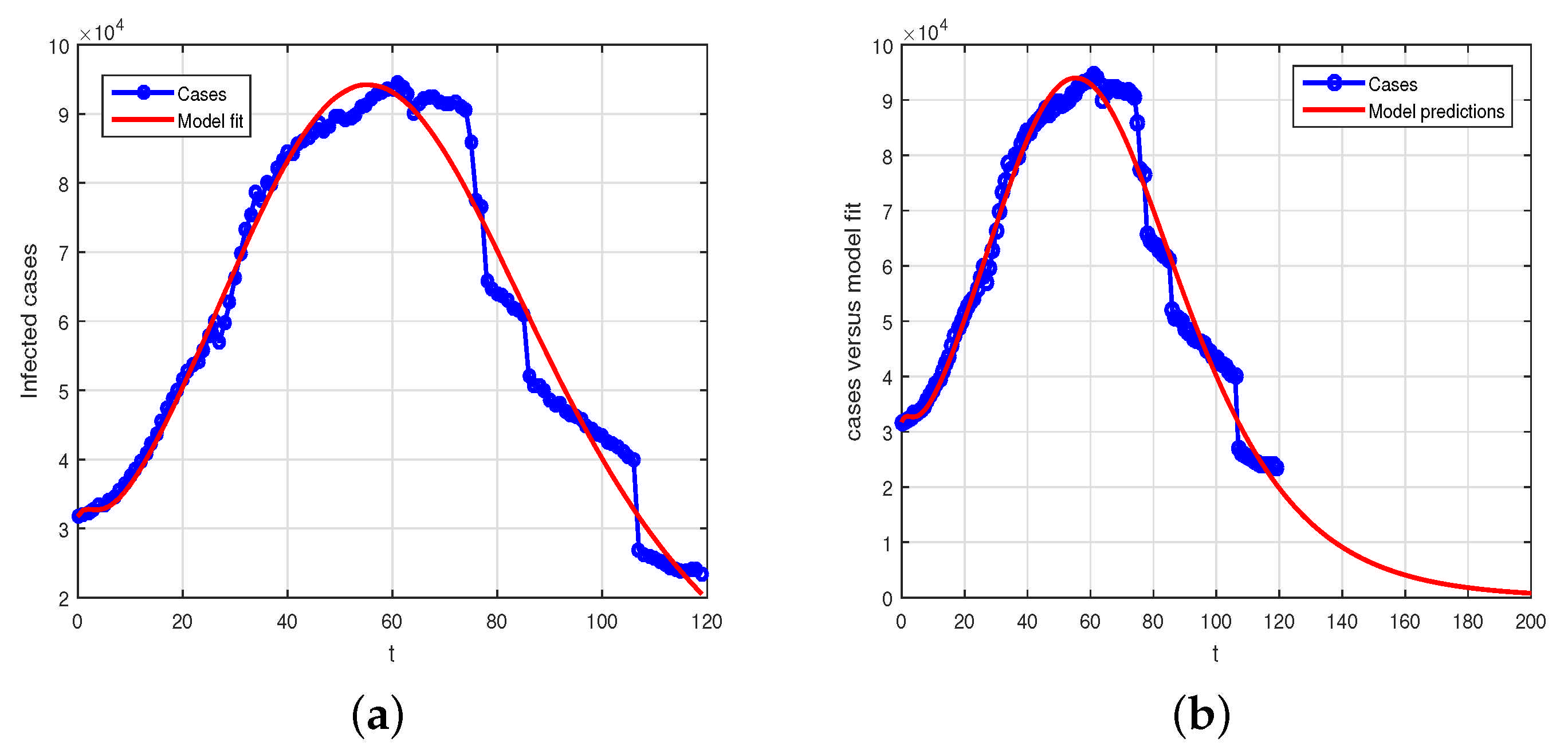The data set versus the model using the nonlinear least square curve fitting has been used and the desired results is shown in Figure 1. In Figure 1a is the model fitting versus data while Figure 1b shows the predictions of the model versus data.

5. Numerical Results and Discussion

Here, we first explain the numerical scheme for the fractional model in terms of the Caputo derivative given in (4). Considering the Adams–Bashforth–Moulten method given in [28,29] to obtain the numerical scheme for the model (4). After implementing the numerical scheme we will consider the real parameters given in Table 1 using the fractional-order $\varpi$ values and present the results.

Numerical Scheme for Model (4)

To implement the Adamas-Bashforth-molten for the system (4), we first re-write the original model in the following shape:

$$\left\{\begin{array}{c}{}^C{D}_t^{\varpi }z\left(t\right)=g(t,z\left(t\right)),0<t<T\hfill \\ z^{\left(r\right)}\left(0\right)=z_0^{\left(r\right)},\hspace{1em}r=0,1,\dots ,\chi ,\hspace{1em}\chi =\left[\varpi \right].\hfill \end{array}\right.$$

(11)

Equation (11) is equivalent to Volterra integral equation given by

$$z\left(t\right)=\sum _{r=0}^{\chi -1}{z}_0^{\left(r\right)}\frac{t^r}{r!}+\frac{1}{\mathrm{\Gamma }\left(\varpi \right)}{\int }_0^t{(t-u)}^{\varpi -1}g(s,z\left(s\right))ds$$

(12)

To integrate (12), we follow the results from [28,29], where the authors used the Adams–Bashforth–Moulton method by setting $h=\frac{T}{N}$, $t_m=mh$, $m=0,1,\dots ,N\in Z^{+}$. So, we write in view of the above-mentioned work [28,29], and the recently used by the scheme given in [14], the fractional model (4) has the following scheme:

$$\begin{array}{ccc}\hfill S_{m+1}& =& S_0+\frac{h^{\varpi }}{\mathrm{\Gamma }(\varpi +2)}\left[\mathrm{\Lambda }-\lambda S^p-\mu S^p\right]+\frac{h^{\varpi }}{\mathrm{\Gamma }(\varpi +2)}\sum _{j=0}^m{a}_{j,m+1}\left[\mathrm{\Lambda }-\lambda S_j-\mu S_j\right],\hfill \\ \hfill E_{m+1}& =& E_0+\frac{h^{\varpi }}{\mathrm{\Gamma }(\varpi +2)}\left[\lambda S^p-{\tau }_1{E}^p\right]+\frac{h^{\varpi }}{\mathrm{\Gamma }(\varpi +2)}\sum _{j=0}^m{a}_{j,m+1}\left[\lambda S_j-{\tau }_1{E}_j\right],\hfill \\ \hfill A_{m+1}& =& A_0+\frac{h^{\varpi }}{\mathrm{\Gamma }(\varpi +2)}\left[\eta \nu E^p-{\tau }_2{A}^p\right]+\frac{h^{\varpi }}{\mathrm{\Gamma }(\varpi +2)}\sum _{j=0}^m{a}_{j,m+1}\left[\eta \nu E_j-{\tau }_2{A}_j\right],\hfill \\ \hfill I_{m+1}& =& I_0+\frac{h^{\varpi }}{\mathrm{\Gamma }(\varpi +2)}\left[(1-\nu )\eta E^p-{\tau }_3{I}^p\right]+\frac{h^{\varpi }}{\mathrm{\Gamma }(\varpi +2)}\sum _{j=0}^m{a}_{j,m+1}\left[(1-\nu )\eta E_j-{\tau }_3{I}_j\right],\hfill \\ \hfill H_{m+1}& =& H_0+\frac{h^{\varpi }}{\mathrm{\Gamma }(\varpi +2)}\left[\kappa I^p-{\tau }_4{H}^p\right]+\frac{h^{\varpi }}{\mathrm{\Gamma }(\varpi +2)}\sum _{j=0}^m{a}_{j,m+1}\left[\kappa I_j-{\tau }_4{H}_j\right],\hfill \\ \hfill R_{m+1}& =& R_0+\frac{h^{\varpi }}{\mathrm{\Gamma }(\varpi +2)}\left[q_1{A}^p+q_2{I}^p+q_3{H}^p-\mu R^p\right]\hfill \\ & & +\frac{h^{\varpi }}{\mathrm{\Gamma }(\varpi +2)}\sum _{j=0}^m{a}_{j,m+1}\left[q_1{A}_j+q_2{I}_j+q_3{H}_j-\mu R_j\right],\hfill \end{array}$$

(13)

where

$$\begin{array}{ccc}\hfill S_{m+1}^p\left(t\right)& =& S_0+\frac{1}{\mathrm{\Gamma }\left(\varpi \right)}\sum _{j=0}^m{∆}_{j,m+1}\left\{\mathrm{\Lambda }-\lambda S_j-\mu S_j\right\},\hfill \\ \hfill E_{m+1}^p\left(t\right)& =& E_0+\frac{1}{\mathrm{\Gamma }\left(\varpi \right)}\sum _{j=0}^m{∆}_{j,m+1}\left\{\lambda S_j-{\tau }_1{E}_j\right\},\hfill \\ \hfill A_{m+1}^p\left(t\right)& =& A_0+\frac{1}{\mathrm{\Gamma }\left(\varpi \right)}\sum _{j=0}^m{∆}_{j,m+1}\left\{\eta \nu E_j-{\tau }_2{A}_j\right\},\hfill \\ \hfill I_{m+1}^p\left(t\right)& =& I_0+\frac{1}{\mathrm{\Gamma }\left(\varpi \right)}\sum _{j=0}^m{∆}_{j,m+1}\left\{(1-\nu )\eta E_j-{\tau }_3{I}_j\right\},\hfill \\ \hfill H_{m+1}^p\left(t\right)& =& H_0+\frac{1}{\mathrm{\Gamma }\left(\varpi \right)}\sum _{j=0}^m{∆}_{j,m+1}\left\{\kappa I_j-{\tau }_4{H}_j\right\},\hfill \\ \hfill R_{m+1}^p\left(t\right)& =& R_0+\frac{1}{\mathrm{\Gamma }\left(\varpi \right)}\sum _{j=0}^m{∆}_{j,m+1}\left\{q_1{A}_j+q_2{I}_j+q_3{H}_j-\mu R_j\right\},\hfill \end{array}$$

where

$$a_{j,m+1}=\left\{\begin{array}{c}{m}^{\varpi +1}-\left(m-\varpi \right){(m+1)}^{\varpi }, j=0,\hfill \\ {(m-j+2)}^{\varpi +1}+{(m-j)}^{\varpi +1}-2{(m-j+1)}^{\varpi +1}, 1\le j\le m,\hfill \\ 1, j=m+1\hfill \end{array}\right.$$

and

$${∆}_{j,m+1}=\frac{h^{\varpi }}{\varpi }\left({(m-j+1)}^{\varpi }-{(m-j)}^{\varpi }\right),\hspace{1em}0\le j\le m.$$

We consider the fractional order model considered in Caputo derivative given in (4) using the numerical values of the model parameters given in Table 1 to obtain the graphical results by the scheme presented above. The numerical scheme, consider for the Caputo fractional order given by (13) is considered and the respective results are shown graphically in Figure 2, Figure 3 and Figure 4. We produced Figure 2 by considering the fractional-order parameter $\phi$ with its different values and presented their results. Figure 2 demonstrates the graphical results for the endemic equilibrium point where the number of susceptible and recovered peoples increases with the decrease in the fractional-order parameters while an increase was observed for the infected compartments of the model. Further, we studied, graphically, the impact of the sensitive and important parameters of the model as shown in Figure 3 and Figure 4. The impact of the contact parameters ${\beta }_1,{\beta }_2,{\beta }_3$ and ${\beta }_4$ with different values on the model (4) is shown in Figure 3. Decreasing the contacts among the healthy with exposed, with asymptomatic, with symptomatic and those with hospitalized individuals can efficiently decrease the populations of infected people and reduce the disease burden on the populations. The impact of the parameters $\eta$, $\nu$ and $\kappa$ with many values can decrease the infected populations, as shown in Figure 4. Facilitating the people by increasing the testing facility and to identify the asymptomatic individuals and to isolate can decrease the further infection of the disease in the country. Upon testing, positive individuals with severe illness should be hospitalized and the treatment of such infected people is the best method to decrease the population of infected people.

6. Conclusions

A new mathematical model to illustrate the dynamics of COVID-19 with the interaction of exposed, asymptomatic, symptomatic and hospitalized individuals in terms of the fractional-order Caputo derivative has been investigated. It is well known that individuals become infected with COVID-19 due to contact with asymptomatic, symptomatic, and hospitalized infected individuals, as well as those who have been exposed to it. It is noted that many health workers and doctors and those working in the management of hospitals died. We discussed the formulations of the problem and then obtained the related properties of the model mathematically. We studied the model to obtain its stability analysis on the basis of the basic reproduction number ${\mathcal{R}}_0$. We found that the model in the disease-free case is locally asymptotically stable whenever ${\mathcal{R}}_0<1$. The global asymptotic stability was proven for the model when ${\mathcal{R}}_0<1$. Further, we the data to be valid from 1 July 2021 to 28 October 2021 and we parameterized the model. The parameters obtained using the nonlinear least-square fitting has been used to obtain the numerical solutions graphically. The impact of the various parameters on the model equations has been discussed and shown graphically. It can be observed from the numerical results that the infection can be eliminated faster if the exposed cases, the identification of asymptomatic cases, the infected cases and those hospitalized or quarantined at home restrict their contact with healthy individuals. The testing facility of the audiovisuals should be increased and those identified as asymptomatic infected should be quarantined in order to decrease the burden and the future wave of infection in the country.

References

1. Active Cases in Pakistan, Worldometers. Available online: https://www.worldometers.info/coronavirus/country/pakistan (accessed on 3 October 2021).
2. Sarkar, K.; Khajanchi, S.; Nieto, J.J. Modeling and forecasting the COVID-19 pandemic in India. Chaos Solitons Fractals 2020, 139, 110049. [Google Scholar] [CrossRef]
3. López, L.; Rodo, X. A modified SEIR model to predict the COVID-19 outbreak in Spain and Italy: Simulating control scenarios and multi-scale epidemics. Results Phys. 2021, 21, 103746. [Google Scholar] [CrossRef] [PubMed]
4. Ullah, S.; Khan, M.A. Modeling the impact of non-pharmaceutical interventions on the dynamics of novel coronavirus with optimal control analysis with a case study. Chaos Solitons Fractals 2020, 139, 110075. [Google Scholar] [CrossRef]
5. Okuonghae, D.; Omame, A. Analysis of a mathematical model for COVID-19 population dynamics in Lagos, Nigeria. Chaos Solitons Fractals 2020, 139, 110032. [Google Scholar] [CrossRef] [PubMed]
6. Sun, T.; Wang, Y. Modeling COVID-19 epidemic in Heilongjiang province, China. Chaos Solitons Fractals 2020, 138, 109949. [Google Scholar] [CrossRef] [PubMed]
7. Deressa, C.T.; Duressa, G.F. Modeling and optimal control analysis of transmission dynamics of COVID-19: The case of Ethiopia. Alex. Eng. J. 2021, 60, 719–732. [Google Scholar] [CrossRef]
8. Alguliyev, R.; Aliguliyev, R.; Yusifov, F. Graph modelling for tracking the COVID-19 pandemic spread. Infect. Dis. Model. 2021, 6, 112–122. [Google Scholar] [CrossRef] [PubMed]
9. Tripathi, A.; Tripathi, R.N.; Sharma, D. A mathematical model to study the COVID-19 pandemic in India. In Modeling Earth Systems and Environment; Springer: Cham, Switzerland, 2021; pp. 1–12. [Google Scholar]
10. Asamoah, J.K.K.; Okyere, E.; Abidemi, A.; Moore, S.E.; Sun, G.Q.; Jin, Z.; Acheampong, E.; Gordon, J.F. Optimal control and comprehensive cost-effectiveness analysis for COVID-19. arXiv 2021, arXiv:2107.09595. [Google Scholar]
11. Du, M.; Wang, Z.; Hu, H. Measuring memory with the order of fractional derivative. Sci. Rep. 2013, 3, 1–3. [Google Scholar] [CrossRef]
12. Gao, W.; Veeresha, P.; Baskonus, H.M.; Prakasha, D.; Kumar, P. A new study of unreported cases of 2019-nCOV epidemic outbreaks. Chaos Solitons Fractals 2020, 138, 109929. [Google Scholar] [CrossRef]
13. Gao, W.; Veeresha, P.; Prakasha, D.; Baskonus, H.M. Novel dynamic structures of 2019-nCoV with nonlocal operator via powerful computational technique. Biology 2020, 9, 107. [Google Scholar] [CrossRef]
14. Tuan, N.H.; Mohammadi, H.; Rezapour, S. A mathematical model for COVID-19 transmission by using the Caputo fractional derivative. Chaos Solitons Fractals 2020, 140, 110107. [Google Scholar] [CrossRef] [PubMed]
15. Baleanu, D.; Mohammadi, H.; Rezapour, S. A fractional differential equation model for the COVID-19 transmission by using the Caputo–Fabrizio derivative. Adv. Differ. Equations 2020, 2020, 1–27. [Google Scholar] [CrossRef] [PubMed]
16. Sene, N. SIR epidemic model with Mittag–Leffler fractional derivative. Chaos Solitons Fractals 2020, 137, 109833. [Google Scholar] [CrossRef]
17. Atangana, A.; Araz, S.İ. Mathematical model of COVID-19 spread in Turkey and South Africa: Theory, methods, and applications. Adv. Differ. Equations 2020, 2020, 1–89. [Google Scholar] [CrossRef] [PubMed]
18. Chu, Y.M.; Ali, A.; Khan, M.A.; Islam, S.; Ullah, S. Dynamics of fractional order COVID-19 model with a case study of Saudi Arabia. Results Phys. 2021, 21, 103787. [Google Scholar] [CrossRef]
19. Odaka, M.; Inoue, K. Modeling viral dynamics in SARS-CoV-2 infection based on differential equations and numerical analysis. Heliyon 2021, 7, e08207. [Google Scholar] [CrossRef] [PubMed]
20. Chatterjee, A.N.; Al Basir, F.; Almuqrin, M.A.; Mondal, J.; Khan, I. SARS-CoV-2 infection with lytic and non-lytic immune responses: A fractional order optimal control theoretical study. Results Phys. 2021, 26, 104260. [Google Scholar] [CrossRef] [PubMed]
21. Ngonghala, C.N.; Iboi, E.; Eikenberry, S.; Scotch, M.; MacIntyre, C.R.; Bonds, M.H.; Gumel, A.B. Mathematical assessment of the impact of non-pharmaceutical interventions on curtailing the 2019 novel Coronavirus. Math. Biosci. 2020, 325, 108364. [Google Scholar] [CrossRef]
22. Srivastava, H.M.; Mohammed, P.O.; Ryoo, C.S.; Hamed, Y. Existence and uniqueness of a class of uncertain Liouville-Caputo fractional difference equations. J. King Saud Univ.-Sci. 2021, 33, 101497. [Google Scholar] [CrossRef]
23. Vargas-De-León, C. Volterra-type Lyapunov functions for fractional-order epidemic systems. Commun. Nonlinear Sci. Numer. Simul. 2015, 24, 75–85. [Google Scholar] [CrossRef]
24. Van den Driessche, P.; Watmough, J. Reproduction numbers and sub-threshold endemic equilibria for compartmental models of disease transmission. Math. Biosci. 2002, 180, 29–48. [Google Scholar] [CrossRef]
25. La Salle, J.P. An Invariance Principle in the Theory of Stability; Center for Dynamical Systems/Brown University: Providence, RI, USA, 1966. [Google Scholar]
26. Pakistan Population, 1950–2020. Available online: https://www.worldometers.info/world-population/pakistan-population (accessed on 1 October 2021).
27. Iboi, E.A.; Ngonghala, C.N.; Gumel, A.B. Will an imperfect vaccine curtail the COVID-19 pandemic in the US? Infect. Dis. Model. 2020, 5, 510–524. [Google Scholar] [PubMed]
28. Diethelm, K.; Ford, N.J. Analysis of fractional differential equations. J. Math. Anal. Appl. 2002, 265, 229–248. [Google Scholar] [CrossRef] [Green Version]
29. Diethelm, K.; Ford, N.J.; Freed, A.D. A predictor-corrector approach for the numerical solution of fractional differential equations. Nonlinear Dyn. 2002, 29, 3–22. [Google Scholar] [CrossRef]
Figure 1. (a) Real data versus model fitting, (b) model predictions.
Fractalfract 05 00271 g001
Figure 2. Simulation of model variables with different values of ϖ = 1 , 0.97 , 0.95 , 0.93 , where sub-figures describe, (a) susceptible individuals, (b) exposed individuals, (c) asymptomatic individuals, (d) symptomatic individuals, (e) hospitalized individuals, (f) recovered individuals.
Fractalfract 05 00271 g002
Figure 3. The impact of contact parameters on the infected population, where sub-figures describe, (a) β 1 = 0.7085 , 0.6985 , 0.6885 , 0.6785 , (b) β 2 = 0.03 , 0.028 , 0.024 , 0.02 , (c) β 3 = 0.2784 , 0.1784 , 0.0784 , (d) β 4 = 0.03 , 0.02 , 0.01 .
Fractalfract 05 00271 g003
Figure 4. The impact of parameters η , ν and κ on the infected individuals, where sub-graphs describe (a) η = 0.8036 , 0.7836 , 0.7436 , (b) ν = 0.8887 , 0.8487 , 0.8087 , (c) κ = 0.2 , 0.3 , 0.4 .
Fractalfract 05 00271 g004