The Influence of Noise on the Exact Solutions of the Stochastic Fractional-Space Chiral Nonlinear Schrödinger Equation

Abstract

In this paper, we consider the stochastic fractional-space Chiral nonlinear Schrödinger equation (S-FS-CNSE) derived via multiplicative noise. We obtain the exact solutions of the S-FS-CNSE by using the Riccati equation method. The obtained solutions are extremely important in the development of nuclear medicine, the entire computer industry and quantum mechanics, especially in the quantum hall effect. Moreover, we discuss how the multiplicative noise affects the exact solutions of the S-FS-CNSE. This equation has never previously been studied using a combination of multiplicative noise and fractional space.

1. Introduction

The fractional derivatives may be used to represent many physical phenomena in electromagnetic theory, signal processing, mathematical biology, engineering applications and different scientific disciplines. For example, the fractional derivative has been utilized in the disciplines of finance [1,2,3], biology [4,5,6], physics [7,8,9,10,11], hydrology [12,13] and biochemistry and chemistry [14,15]. Since fractional-order integrals and derivatives allow for the representation of the memory and heredity properties of various substances, these new fractional-order models are more suited than the previously used integer-order models [16]. This is the most important benefit of fractional-order models in comparison with integer-order models, where such impacts are ignored.

On the other hand, randomness or fluctuations have now been shown to be important in many phenomena. Therefore, random effects have become significant when modeling different physical phenomena that take place in oceanography, physics, biology, meteorology, environmental sciences, and so on. Equations that consider random fluctuations in time are referred to as stochastic differential equations.

It seems to be more important to examine fractional equations with some random force. Therefore, in this paper, we take into account the following stochastic fractional-space Chiral nonlinear Schrödinger equation (S-FS-CNSE) derived in the Itô sense by multiplicative noise in this form

$$i{\phi }_t+D_x^{2\alpha }\phi -i\delta ({\phi }^{*}{D}_x^{\alpha }\phi -\phi D_x^{\alpha }{\phi }^{*})\phi =i\rho \phi W_t,$$

(1)

where $\phi (x,t)$ is a complex function, $\rho$ is the noise strength, W is the standard Gaussian process, $\delta$ is a nonlinear coupling constant and the symbol ∗ indicates the complex conjugate. In this study, we restrict ourselves to the case of spatially constant noise.

Equation (1) with $\rho =0$ is a kind of nonlinear evolution equation found in many fields of applied research, including nonlinear quantum mechanics, plasma physics, and optics. It produces chiral solitons, which play a significant role in the quantum-hall effect. Recently, many authors addressed Equation (1) with $\alpha =1$ and $\rho =0$, such as Nishino et al. [17] Bulut et al. [18], Rezazadeh et al. [19], Javid and Raza [20], Eslami [21], Biswas et al. [22], Cheemaa et al. [23], Alshahrani et al. [24], Sulaiman et al. [25] and Rehman et al. [26], while Mohammed et al. [27,28] studied Equation (1) in one space dimension and two space dimensions, with stochastic term and $\alpha =1.$

The originality of this article is to obtain the exact stochastic fractional solutions of the S-FS-CNSE (1) forced by multiplicative noise by using the Riccati equation method. In addition, we discuss the influence of the stochastic term on these solutions. To add more to our knowledge, this is the first paper that uses a combination of multiplicative noise and fractional space to obtain the exact solution of the S-FS-CNSE (1).

The following is the format of this article: In the next section, we define the order $\alpha$ of Jumarie’s derivative and we state some important properties of the modified Riemann–Liouville derivative. In Section 3, we obtain the wave equation for S-FS-CNSE (1), while in Section 4, we have the exact stochastic solutions of the S-FS-CNSE (1) by applying the Riccati equation method. In Section 6, we display some graphs to demonstrate the effect of the stochastic term on the obtained solutions of the S-FS-CNSE. Finally, the conclusions of this paper are presented.

2. Modified Riemann–Liouville Derivative and Properties

Jumarie [29] defines the order $\alpha$ of derivative for the continuous function f: $\mathbb{R}\to \mathbb{R}$ as follows:

$$D_x^{\alpha }f\left(x\right)=\left\{\begin{array}{l}\frac{1}{\Gamma (1-\alpha )}\frac{d}{dx}{\int }_0^x{(x-\zeta )}^{-\alpha }(f\left(\zeta \right)-f\left(0\right))d\zeta ,0<\alpha <1,\\ \\ [f^{\left(n\right)}{\left(x\right)]}^{\alpha -n},n\le \alpha \le n+1,n\ge 1,\end{array}\right.$$

where $\Gamma (.)$ is the Gamma function.

Here, we present some important properties of the modified Riemann–Liouville derivative:

$$D_x^{\alpha }{x}^{\gamma }=\frac{\Gamma (1+\gamma )}{\Gamma (1+\gamma -\alpha )}{x}^{\gamma -\alpha },\gamma >0,$$

$$\begin{array}{ccc}\hfill D_x^{\alpha }[af\left(x\right)+bg\left(x\right)]& =& a{D}_x^{\alpha }f\left(x\right)+b{D}_x^{\alpha }g\left(x\right),\hfill \\ & \end{array}$$

$$D_x^{\alpha }\left[f\left(x\right)g\left(x\right)\right]={\sigma }_x[g\left(x\right)D_x^{\alpha }f\left(x\right)+f\left(x\right)D_x^{\alpha }g\left(x\right)$$

and

$$D_x^{\alpha }g\left(\phi \left(x\right)\right)={\sigma }_x\frac{dg}{d\phi }{D}_x^{\alpha }\phi ,$$

where $a,b$ are constants and ${\sigma }_x$ is called the sigma indexes [30,31].

3. Wave Equation for S-FS-CNSE Equation

Let us begin with the complex wave transformation:

$$\phi (t,x)=\psi \left(\xi \right)e^{i\theta +\rho W\left(t\right)-{\rho }^{2}t},\xi =\frac{k_1{x}^{\alpha }}{\Gamma (1+\alpha )}+k_{2}t,\mathrm{and}\theta =\frac{{\omega }_1{x}^{\alpha }}{\Gamma (1+\alpha )}+{\omega }_{2}t,$$

(2)

where $\psi$ is a determinstic function, $k_1,k_2,$${\omega }_1$ and ${\omega }_2$ are real constants. We use

$$\begin{array}{ccc}\hfill \frac{d\phi }{dt}& =& (k_2{\psi }^{\prime }+i{\omega }_2\psi +\rho \psi W_t+\frac{1}{2}{\rho }^2\psi -{\rho }^2\psi )e^{i\theta +\rho W\left(t\right)-{\rho }^{2}t},\hfill \\ \hfill D_x^{\alpha }\phi & =& ({\sigma }_x{k}_1{\psi }^{\prime }+i{\sigma }_x{\omega }_1\psi )e^{i\theta +\rho W\left(t\right)-{\rho }^{2}t},\hfill \\ \hfill D_x^{\alpha }{\phi }^{*}& =& ({\sigma }_x{k}_1{\psi }^{\prime }-i{\sigma }_x{\omega }_1\psi )e^{-i\theta +\rho W\left(t\right)-{\rho }^{2}t},\hfill \\ \hfill D_x^{2\alpha }\phi & =& ({\sigma }_x^2{k}_1^2{\psi }^{″}+2i{\sigma }_x^2{k}_1{\omega }_1{\psi }^{\prime }-{\sigma }_x^2{\omega }_1^2\psi )e^{i\theta +\rho W\left(t\right)-{\rho }^{2}t}.\hfill \end{array}$$

(3)

Putting (3) into Equation (1), we obtain, for real part,

$${\sigma }_x^2{k}_1^2{\psi }^{″}+2\delta {\sigma }_x{\omega }_1{\psi }^3{e}^{2\rho W\left(t\right)-2{\rho }^{2}t}-({\omega }_2+{\sigma }_x^2{k}_1^2)\psi =0.$$

(4)

Taking expectation on both sides, we have

$${\sigma }_x^2{k}_1^2{\psi }^{″}+2\delta {\sigma }_x{\omega }_1{\psi }^3{e}^{-2{\rho }^{2}t}\mathbb{E}\left(e^{2\sigma W\left(t\right)}\right)-({\omega }_2+{\sigma }_x^2{k}_1^2)\psi =0,$$

(5)

where $\psi$ is a deterministic function. Since $W\left(t\right)$ is standard normal random variable, then $\mathbb{E}\left(e^{\gamma W\left(t\right)}\right)=e^{\frac{{\gamma }^2}{2}t}$ for any real constant $\gamma .$ Hence Equation (5) becomes

$${\psi }^{″}+H_1{\psi }^3-H_2\psi =0,$$

(6)

where $H_1=\frac{2\delta {\omega }_1}{{\sigma }_x{k}_1^2}$ and $H_2=\frac{{\omega }_2+{\sigma }_x^2{k}_1^2}{{\sigma }_x^2{k}_1^2}.$

In the next, we utiliz the Riccati equation method to find the exact solution of the S-FS-CNSE (1).

4. The Exact Solutions of the S-FS-CNSE

Here, we apply the Riccati equation method to find the solutions of Equation (6). That leads us to find the exact solutions of the S-FS-CNSE (1). First, we suppose the solution of the (6) has the form

$$\psi =\sum _{\ell =0}^N{a}_{\ell }{\chi }^{\ell },$$

(7)

where $\chi$ solves

$${\chi }^{\prime }={\chi }^2+b,$$

(8)

where b is an unknown constant. By balancing ${\psi }^3$ with ${\psi }^{″}$ in Equation (6), we can evaluate the parameter N as follows:

$$3N=N+2,$$

hence

$$N=1.$$

(9)

From Equation (9), we can rewrite Equation (7) as

$$\psi =a_0+a_1\chi ,a_1\ne 0.$$

(10)

Putting Equation (10) into Equation (6) and utilizing Equation (8), we obtain a polynomial with degree 3 of $\chi$ as follows:

$$\begin{array}{ccc}& & (2a_1+H_1{a}_1^3){\chi }^3+\left(H_1{a}_0{a}_1^2\right){\chi }^2\hfill \\ & & +(2a_{1}b+H_1{a}_0^2{a}_1-H_2{a}_1)\chi +H_1{a}_0^3-H_2{a}_0=0\hfill \end{array}$$

Equating each coefficient of ${\chi }^k$ ($k=3,2,1,0$) to zero, we have the set of algebraic equations as follows:

$$2a_1+H_1{a}_1^3=0,$$

$$H_1{a}_0{a}_1^2=0,$$

$$2a_{1}b+H_1{a}_0^2{a}_1-H_2{a}_1=0,$$

and

$$H_1{a}_0^3-H_2{a}_0=0.$$

By solving this system, we obtain:

$$a_0=0,a_1=\pm \sqrt{\frac{-2}{H_1}}\mathrm{and}b=\frac{H_2}{2}.$$

There many cases for the solutions of Equation (8) depend on b.

First case: If ${\omega }_2=-{\sigma }_x^2{k}_1^2$, then $b=0$. The solution of Equation (8) in this case becomes

$$\chi \left(\xi \right)=\frac{-1}{\xi }.$$

According to Equation (10), the corresponding solution of the traveling wave Equation (6) is

$$\psi \left(\xi \right)=\pm \sqrt{\frac{-2}{H_1}}{\xi }^{-1}\mathrm{if}{H}_1<0,$$

or

$$\psi \left(\xi \right)=\pm i\sqrt{\frac{2}{H_1}}{\xi }^{-1}\mathrm{if}{H}_1>0.$$

Therefore, the exact solution of the S-FS-CNSE (1) is

$${\phi }_1(x,t)=\pm \sqrt{\frac{-2}{H_1}}{(\frac{k_1{x}^{\alpha }}{\Gamma (1+\alpha )}+k_{2}t)}^{-1}{e}^{i(\frac{{\omega }_1{x}^{\alpha }}{\Gamma (1+\alpha )}+{\omega }_{2}t)+\rho W\left(t\right)-{\rho }^{2}t}\mathrm{if}{H}_1<0,$$

(11)

or

$${\phi }_2(x,t)=\pm i\sqrt{\frac{2}{H_1}}{(\frac{k_1{x}^{\alpha }}{\Gamma (1+\alpha )}+k_{2}t)}^{-1}{e}^{i(\frac{{\omega }_1{x}^{\alpha }}{\Gamma (1+\alpha )}+{\omega }_{2}t)+\rho W\left(t\right)-{\rho }^{2}t}\mathrm{if}{H}_1>0.$$

(12)

Second case: If ${\omega }_2>-{\sigma }_x^2{k}_1^2$, then $b>0$. The solution of Equation (8) in this case becomes

$$\chi \left(\xi \right)=\sqrt{b}tan\left(\sqrt{b}\xi \right)=\sqrt{\frac{H_2}{2}}tan\left(\sqrt{\frac{H_2}{2}}\xi \right).$$

In this situation, the solution of the traveling wave Equation (6) takes the form

$$\psi \left(\xi \right)=\pm \sqrt{\frac{-H_2}{H_1}}tan\left(\sqrt{\frac{H_2}{2}}\xi \right),\mathrm{if}{H}_1<0,$$

or

$$\psi \left(\xi \right)=\pm i\sqrt{\frac{H_2}{H_1}}tan\left(\sqrt{\frac{H_2}{2}}\xi \right),\mathrm{if}{H}_1>0.$$

Hence, by using (2), the exact solution of the S-FS-CNSE (1) is

$${\phi }_3(x,t)=\pm \sqrt{\frac{-H_2}{H_1}}tan\left(\sqrt{\frac{H_2}{2}}(\frac{k_1{x}^{\alpha }}{\Gamma (1+\alpha )}+k_{2}t)\right)e^{i(\frac{{\omega }_1{x}^{\alpha }}{\Gamma (1+\alpha )}+{\omega }_{2}t)+\rho W\left(t\right)-{\rho }^{2}t},$$

(13)

if$H_1<0,$ or

$${\phi }_4(x,t)=\pm i\sqrt{\frac{H_2}{H_1}}tan\left(\sqrt{\frac{H_2}{2}}(\frac{k_1{x}^{\alpha }}{\Gamma (1+\alpha )}+k_{2}t)\right)e^{i(\frac{{\omega }_1{x}^{\alpha }}{\Gamma (1+\alpha )}+{\omega }_{2}t)+\rho W\left(t\right)-{\rho }^{2}t},$$

(14)

if$H_1>0.$

Third case: If ${\omega }_2<-{\sigma }_x^2{k}_1^2$, then $b<0$. The solution of Equation (8) in this case becomes

$$\chi \left(\xi \right)=\sqrt{-b}tanh\left(\sqrt{-b}\xi \right)=\sqrt{\frac{-H_2}{2}}tanh\left(\sqrt{\frac{-H_2}{2}}\xi \right).$$

In this situation, the solution of the traveling wave Equation (6) takes the form

$$\psi \left(\xi \right)=\pm \sqrt{\frac{H_2}{H_1}}tanh\left(\sqrt{\frac{-H_2}{2}}\xi \right),\mathrm{if}{H}_1<0,$$

or

$$\psi \left(\xi \right)=\pm i\sqrt{\frac{-H_2}{H_1}}tanh\left(\sqrt{\frac{H_2}{2}}\xi \right),\mathrm{if}{H}_1>0.$$

Therefore, by using Equation (2), the exact solution of the S-FS-CNSE (1) is

$${\phi }_5(x,t)=\pm \sqrt{\frac{H_2}{H_1}}tanh\left(\sqrt{\frac{-H_2}{2}}(\frac{k_1{x}^{\alpha }}{\Gamma (1+\alpha )}+k_{2}t)\right)e^{i(\frac{{\omega }_1{x}^{\alpha }}{\Gamma (1+\alpha )}+{\omega }_{2}t)+\rho W\left(t\right)-{\rho }^{2}t}$$

(15)

if$H_1<0,$ or

$${\phi }_6(x,t)=\pm i\sqrt{\frac{-H_2}{H_1}}tan\left(\sqrt{\frac{-H_2}{2}}(\frac{k_1{x}^{\alpha }}{\Gamma (1+\alpha )}+k_{2}t)\right)e^{i(\frac{{\omega }_1{x}^{\alpha }}{\Gamma (1+\alpha )}+{\omega }_{2}t)+\rho W\left(t\right)-{\rho }^{2}t},$$

(16)

if$H_1>0.$

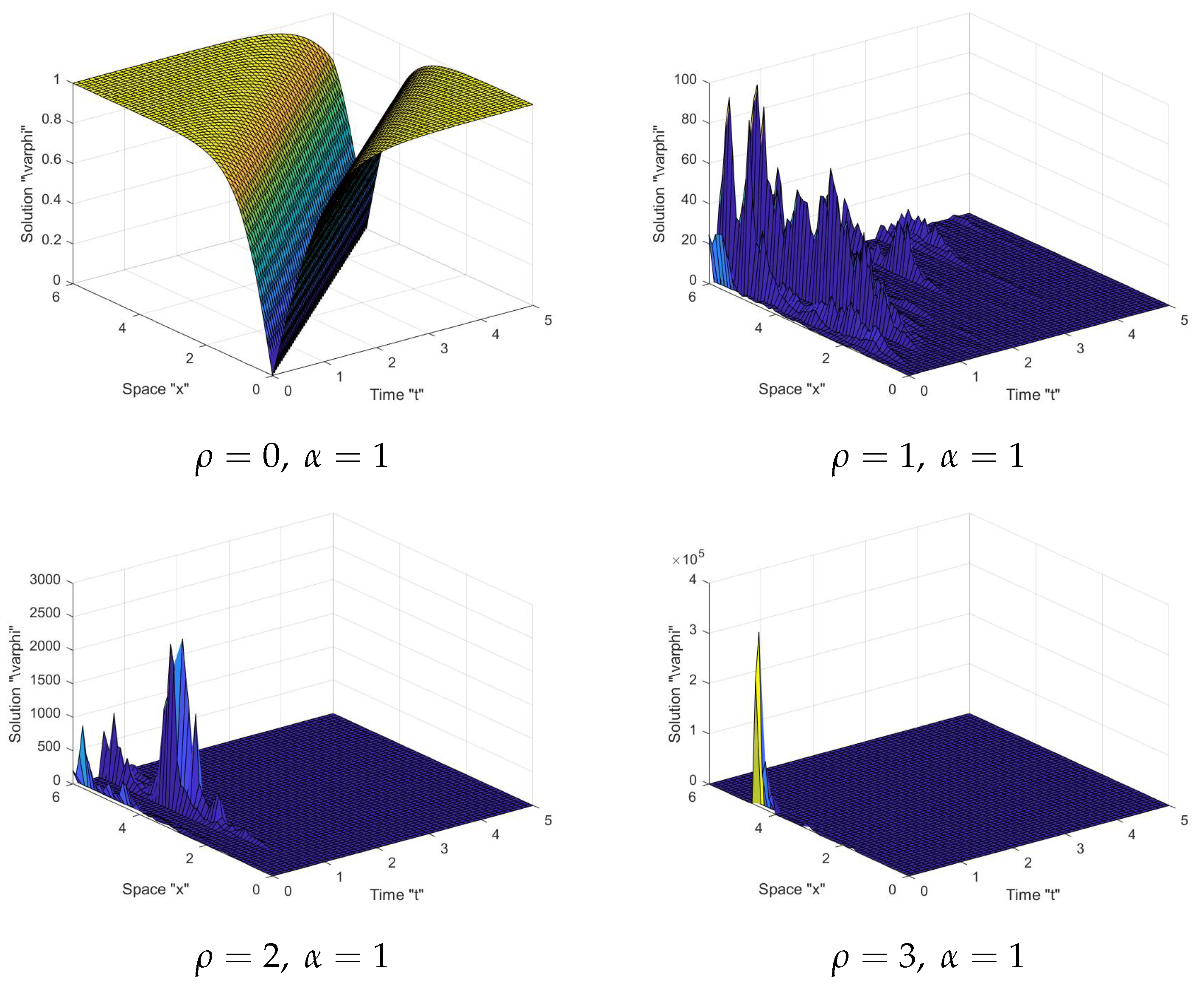
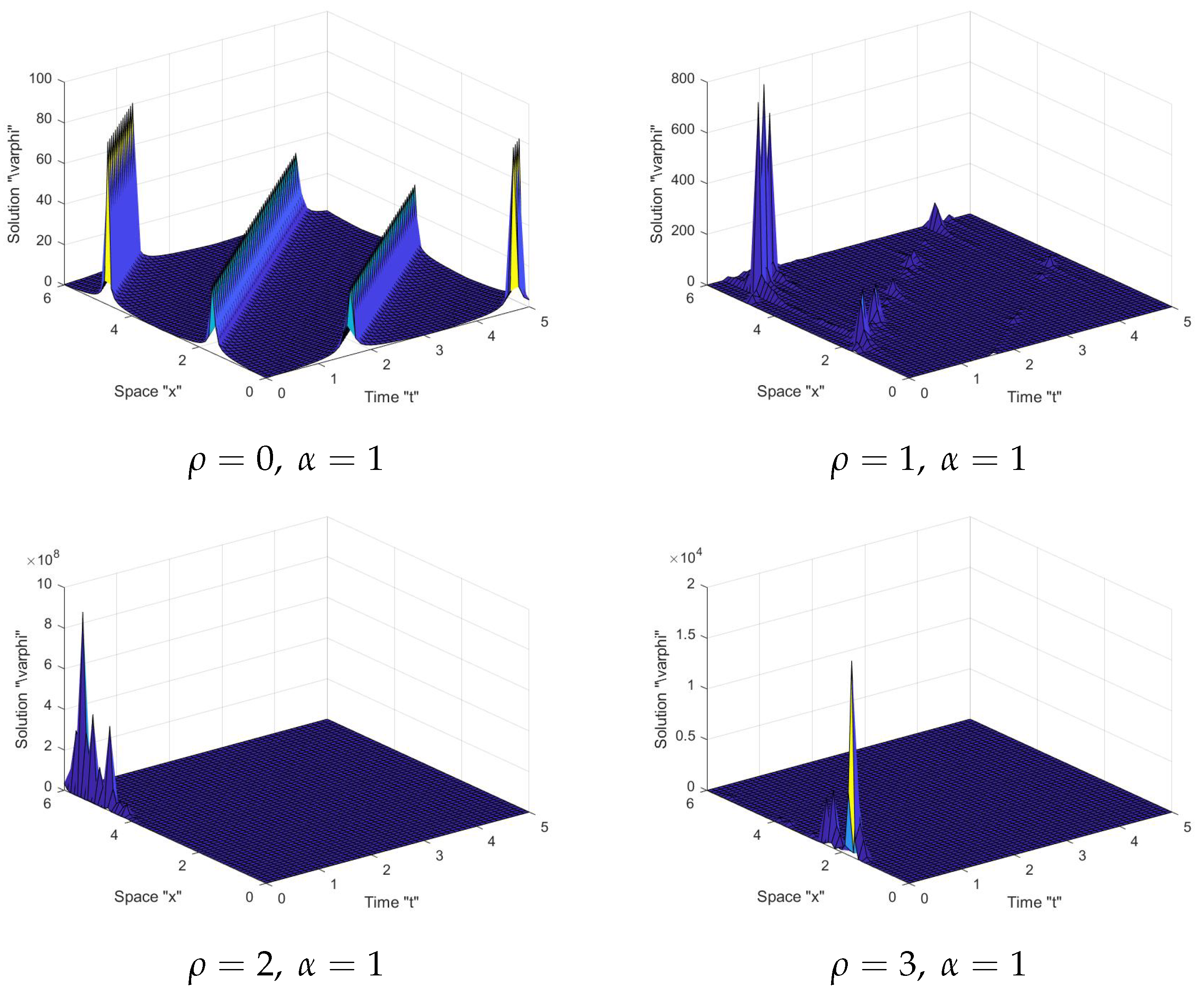
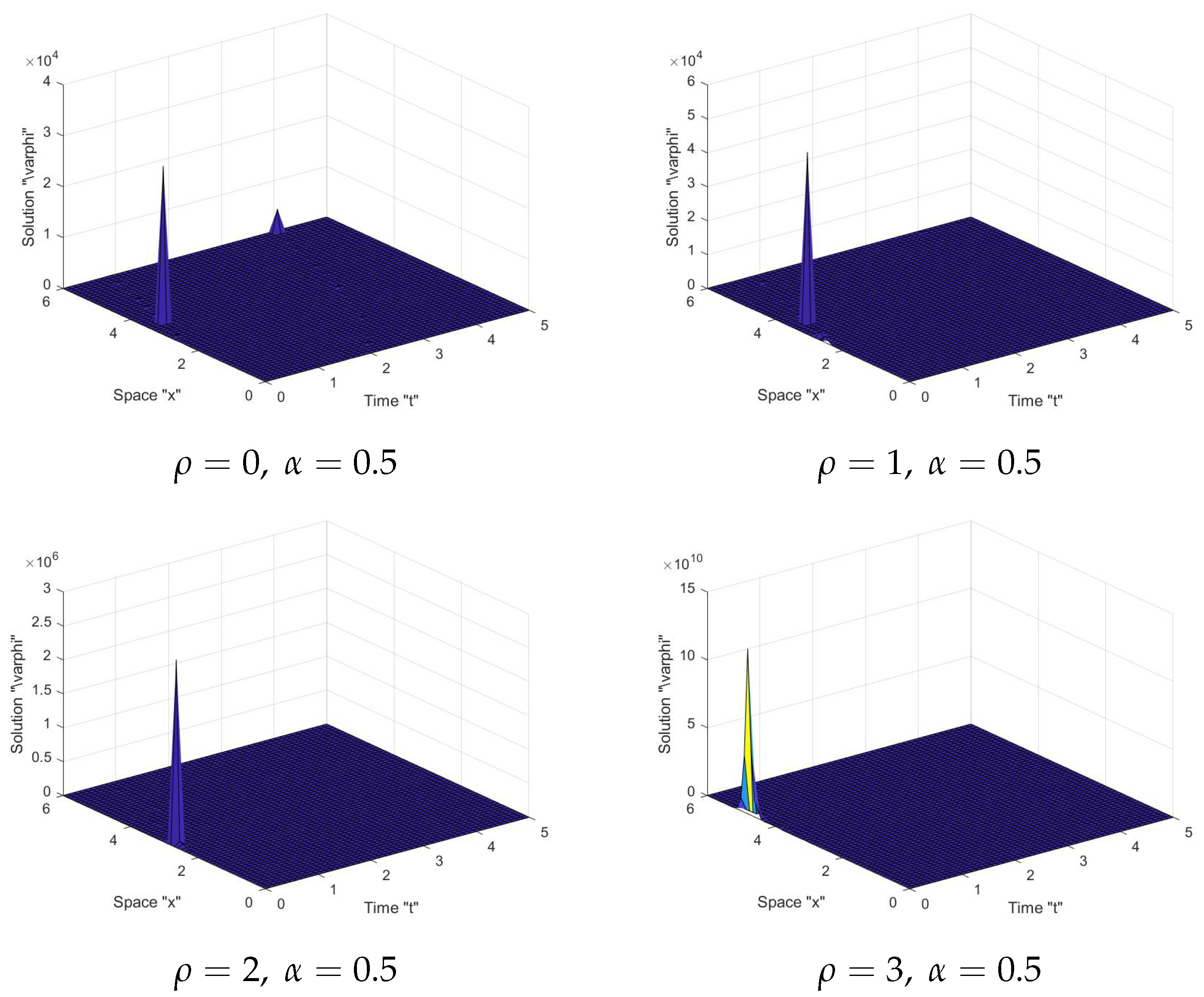
5. The Effect of Noise on the Solutions of S-FS-CNSE

Understanding the influence of noise on wave propagation is a critical issue. Even though deterministic models are frequently used to illustrate propagation, in many cases, randomness should be addressed. It has the potential to significantly modify qualitative behavior and result in new properties. Therefore, in this section, we address the effect of the stochastic term on the exact solutions of the S-FS-CNSE (1).

First, let us fix the parameters $k_1=\delta =\frac{1}{{\sigma }_x}$ and $k_2=-1$. We present some of graphs for different value of $\rho$ (noise intensity). We utilize the MATLAB program to plot the solution ${\phi }_3(t,x)$ and ${\phi }_5(t,x)$ defined in Equations (11) and (13), respectively, as follows.

In Figure 1, Figure 2, Figure 3 and Figure 4: When the noise intensity is equal to zero, the surface becomes less flat, as seen in the first graph in the tables. However, when noise emerges and the intensity of the noise increases ($\rho =1,2,3$), the surface becomes more planar after minor transitioning behaviors. This indicates that the solutions are stable due to the effect of the stochastic term.

6. Conclusions

In this article, we obtained different exact solutions of the stochastic fractional-space Chiral nonlinear Schrödinger equation (Equation (1)) by using the Riccati equation method. We were able to obtain several dark and bright soliton solutions for this equation. These forms of solutions can be used to explain a wide range of exciting and difficult scientific phenomena. Moreover, we utilized the MATLAB program to create some graphical representations to discuss the impact of the stochastic term on the exact solutions of the S-FS-CNSE (1). Finally, we noticed that the proposed method is a simple and beautiful mathematical technique that gives important results when applied to several types of nonlinear models.

References

1. Gorenflo, R.; Mainardi, F. Random walk models for space–fractional diffusion processes. Fract. Calculus Appl. Anal. 1998, 1, 167–191. [Google Scholar]
2. Raberto, M.; Scalas, E.; Mainardi, F. Waiting-times and returns in high-frequency financial data: An empirical study. Phys. A Stat. Its Appl. 2002, 314, 749–755. [Google Scholar] [CrossRef] [Green Version]
3. Wyss, W. The fractional Black–Scholes equation. Fract. Calculus Appl. Anal. 2000, 3, 51–61. [Google Scholar]
4. Yuste, S.B.; Lindenberg, K. Subdiffusion-limited A + A reactions. Phys. Rev. Lett. 2001, 87, 118301. [Google Scholar] [CrossRef] [PubMed] [Green Version]
5. Iqbal, N.; Wu, R.; Mohammed, W.W. Pattern formation induced by fractional cross-diffusion in a 3-species food chain model with harvesting. Math. Comput. Simul. 2021, 188, 102–119. [Google Scholar] [CrossRef]
6. Khater, M.M.A. Novel explicit breath wave and numerical solutions of an Atangana conformable fractional Lotka–Volterra model. Alex. Eng. J. 2021, 60, 4735–4743. [Google Scholar] [CrossRef]
7. Barkai, E.; Metzler, R.; Klafter, J. From continuous time random walks to the fractional Fokker–Planck equation. Phys. Rev. 2000, 61, 132–138. [Google Scholar] [CrossRef]
8. Metzler, R.; Klafter, J. The random walk’s guide to anomalous diffusion: A fractional dynamics approach. Phys. Rep. 2000, 339, 1–77. [Google Scholar] [CrossRef]
9. Saichev, A.I.; Zaslavsky, G.M. Fractional kinetic equations: Solutions and applications. Chaos 1997, 7, 753–764. [Google Scholar] [CrossRef] [PubMed] [Green Version]
10. Mohammed, W.W.; Alesemi, M.; Albosaily, S.; Iqbal, N.; El-Morshedy, M. The exact solutions of stochastic fractional-space Kuramoto-Sivashinsky equation by using (G’/G)-expansion method. Mathematics 2021, 9, 2712. [Google Scholar] [CrossRef]
11. Khater, M.M.A.; Lu, D. Analytical versus numerical solutions of the nonlinear fractional time–space telegraph equation. Mod. Phys. Lett. B 2021, 35, 2150324. [Google Scholar] [CrossRef]
12. Benson, D.A.; Wheatcraft, S.W.; Meerschaert, M.M. The fractional-order governing equation of Lévy motion. Water Resour. Res. 2000, 36, 1413–1423. [Google Scholar] [CrossRef]
13. Liu, F.; Anh, V.; Turner, I. Numerical solution of the space fractional Fokker–Planck equation. J. Comput. Appl. Math. 2004, 166, 209–219. [Google Scholar] [CrossRef] [Green Version]
14. Yuste, S.B.; Acedo, L.; Lindenberg, K. Reaction front in an A + BC reaction–subdiffusion process. Phys. Rev. E 2004, 69, 036126. [Google Scholar] [CrossRef] [PubMed] [Green Version]
15. Mohammed, W.W.; Iqbal, N. Impact of the same degenerate additive noise on a coupled system of fractional space diffusion equations. Fractals 2021, 30, 2240033. [Google Scholar] [CrossRef]
16. Podlubny, I. Fractional Differential Equations; Academic Press: New York, NY, USA, 1999. [Google Scholar]
17. Nishino, A.; Umeno, Y.; Wadati, M. Chiral nonlinear Schrödinger equation. Chaos Solitons Fractals 1998, 9, 1063–1069. [Google Scholar] [CrossRef]
18. Bulut, H.; Sulaiman, T.A.; Demirdag, B. Dynamics of soliton solutions in the chiral nonlinear Schrödinger equations. Nonlinear Dyn. 2018, 91, 1985–1991. [Google Scholar] [CrossRef]
19. Rezazadeh, H.; Younis, M.; Rehman, S.; Eslami, M.; Bilal, M.; Younas, U. New exact traveling wave solutions to the (2+1)-dimensional Chiral nonlinear Schrödinger equation. Math. Model. Nat. Phenom. 2021, 16, 38. [Google Scholar] [CrossRef]
20. Javid, A.; Raza, N. Chiral solitons of the (1 + 2)-dimensional nonlinear Schrodinger’s equation. Mod. Phys. Lett. B 2019, 33, 1950401. [Google Scholar] [CrossRef]
21. Eslami, M. Trial solution technique to chiral nonlinear Schrödinger’s equation in (1 + 2)-dimensions. Nonlinear Dyn. 2016, 85, 813–816. [Google Scholar] [CrossRef]
22. Biswas, A.; Mirzazadeh, M. Dark optical solitons with power law nonlinearity using G′/G-expansion. Optik 2014, 125, 4603–4608. [Google Scholar] [CrossRef]
23. Cheemaa, N.; Chen, S.; Seadawy, A.R. Chiral soliton solutions of perturbed chiral nonlinear Schrödinger equation with its applications in mathematical physics. Int. J. Mod. Phys. B 2020, 34, 2050301. [Google Scholar] [CrossRef]
24. Alshahrani, B.; Yakout, H.A.; Khater, M.M.A.; Abdel-Aty, A.; Mahmoud, E.E.; Baleanu, D.; Eleuch, H. Accurate novel explicit complex wave solutions of the (2+ 1)-dimensional Chiral nonlinear Schrödinger equation. Results Phys. 2021, 23, 104019. [Google Scholar] [CrossRef]
25. Sulaiman, T.A.; Yusuf, A.; Abdel-Khalek, S.; Bayram, M.; Ahmad, H. Nonautonomous complex wave solutions to the (2+1)-dimensional variable-coefficients nonlinear chiral Schrödinger equation. Results Phys. 2020, 19, 103604. [Google Scholar] [CrossRef]
26. Rehman, H.; Imran, M.A.; Bibi, M.; Riaz, M.; Akgül, A. New soliton solutions of the 2D-chiral nonlinear Schrodinger equation using two integration schemes. Math. Methods Appl. Sci. 2021, 44, 5663–5682. [Google Scholar] [CrossRef]
27. Abdelrahman, M.; Mohammed, W.W. The impact of multiplicative noise on the solution of the Chiral nonlinear Schrödinger equation. Phys. Scr. 2020, 95, 085222. [Google Scholar] [CrossRef]
28. Albosaily, S.; Mohammed, W.W.; Aiyashi, M.A. Exact solutions of the (2+ 1)-dimensional stochastic chiral nonlinear Schrödinger equation. Symmetry 2020, 12, 1874. [Google Scholar] [CrossRef]
29. Jumarie, G. Modified Riemann–Liouville derivative and fractional Taylor series of nondifferentiable functions further results. Comput. Math. Appl. 2006, 51, 1367–1376. [Google Scholar] [CrossRef] [Green Version]
30. He, J.H.; Elegan, S.K.; Li, Z.B. Geometrical explanation of the fractional complex transform and derivative chain rule for fractional calculus. Phys. Lett. A 2012, 376, 257–259. [Google Scholar] [CrossRef]
31. Aksoy, E.; Kaplan, M.; Bekir, A. Exponential rational function method for space–time fractional differential equations. Waves Random Complex Media 2016, 26, 142–151. [Google Scholar] [CrossRef]
Figure 1. Graph of solution φ 3 in Equation (13) with ω 1 = 1 , ω 2 = 1 and α = 1 .
Fractalfract 05 00262 g001
Figure 2. Graph of solution φ 3 in Equation (15) with ω 1 = 1 , ω 2 = 1 and α = 0.5 .
Fractalfract 05 00262 g002
Figure 3. Graph of solution φ 5 in Equation (15) with ω 1 = 1 , ω 2 = 2 and α = 1 .
Fractalfract 05 00262 g003
Figure 4. Graph of solution φ 5 in Equation (13) with ω 1 = 1 , ω 2 = 2 and α = 0.5 .
Fractalfract 05 00262 g004
Publisher’s Note: MDPI stays neutral with regard to jurisdictional claims in published maps and institutional affiliations.