Dynamics of Fractional Model of Biological Pest Control in Tea Plants with Beddington–DeAngelis Functional Response

Abstract

In this study, we depicted the spread of pests in tea plants and their control by biological enemies in the frame of a fractional-order model, and its dynamics are surveyed in terms of boundedness, uniqueness, and the existence of the solutions. To reduce the harm to the tea plant, a harvesting term is introduced into the equation that estimates the growth of tea leaves. We analyzed various points of equilibrium of the projected model and derived the conditions for the stability of these equilibrium points. The complex nature is examined by changing the values of various parameters and fractional derivatives. Numerical computations are conducted to strengthen the theoretical findings.

1. Introduction

Tea, the most consumed drink in the world following water, is not only considered a beverage, it is considered a gift to mankind from nature for beginning a fresh day [1]. The majority of tea-producing countries are located in Asia, with India, China, and Sri Lanka being the most prominent producers [2]. All types of tea, whether it be green, white, black or yellow, come from the same plant, Camellia sinensis. Around $52\%$ of the total tea is produced in India, coming from the State of Assam. Tea is grown within the tropics and subtropics in various types of porous, well-drained, acidic soils (PH $3.3$ to $6.0$) in diverse agroecological conditions and undergoes a broad range of climatic conditions such as annual rainfall from 938 to 6000 mm, temperatures from 12 °C to 40 °C, and the relative humidity may vary from 30 percent to 90 percent [3]. Tea trees can grow up to 15 m in height in the wild [4,5].

One of the substantial tasks for tea growers is to fight against diseases and pests as the tea plant can have a life span of around 30 to 50 years [4]. As March to mid-November is the season for the tea planters to harvest the crop, the tea plants will be easily affected by pests as the population of the pests peaks from June to September (see Figure 1). Hence, pests become inevitable guests in every cropping system and reduce plant growth, damage different parts of the plant, reduce the quality of the crop, and ultimately affect the productivity of crop yields [6]. The insects suck the sap from buds, leaves and terminal twigs with the help of their mouth styles, as well as infusing them with their saliva, which is a toxic substance [6]. Because of this, eventually, the fresh and healthy leaves deform and curl up. As a result, the plant begins to die from the tip of its leaves or roots backwards, owing to an unfavorable environment. Each female bug searches for soft plant tissues and lays about 500–600 eggs [7]. After a week, the eggs hatch by releasing the nymphs. For an entire life cycle to complete, it takes almost one month. There can also exist several generations of pests. The paramount damage from pests occurs especially in moist and shaded areas after monsoon showers [4].

As the production of tea plants increases, the magnitude of the losses is also increased simultaneously and productivity is engineered by agro-technology. An individual pest can cause several assessments of crop loss [8]. The national economy of several countries is dependent on its production in several constraints. On average around $5\%$ to $55\%$ of the damage is caused by insects and mite pests (arthropods) [3,5,9,10,11].

There are several strategies to control pests. They are mainly natural control factors and applied control techniques. The natural control factors are climatic factors, topographic features, predators and parasites, and so forth. Similarly, applied control techniques are as follows: Cultural control, Physical control, Biological control, Microbial control, Mechanical control, Regulatory control, Breeding of resistant agrotypes, Chaemosterilant and Chemical control and Ionizing radiation, and so forth [9,11].

At the beginning of tea cultivation, the pests in tea were largely controlled by the use of synthetic insecticides and acaricides. However, the large-scale and continuous use of synthetic pesticides over a long time exerts a harmful impact on human and environmental health. The impact factors of pesticides are the loss of natural antagonists to pests, domestic animal contaminations and deaths, pesticide resistance, losses to adjacent crops, Honeybee and pollination decline, contamination of groundwater, and fishery and bird losses [12]. Due to the death of microorganisms caused by pesticides, the fertility of soil is affected and also pests develop resistance to pesticides, disrupt the natural enemy complex, cause a residue problem and also significant health problems as the products are produced by chemical alteration [13]. Hence, one should definitely choose the alternative option for pest management instead of dependence on pesticides [14].

To protect the plants against pest organisms, nature has its own tactics where biological control is one of the oldest and most eco-friendly techniques in pest management [11,15]. In biological control methods, the pest organisms are controlled by the use of natural enemies instead of using chemical pesticides (see Figure 2). The term "Biological control" signifies the application and utilization of natural enemies to control the pests. Within an agroecosystem, biological control is the one and only method that is an environmentally friendly control method that enhances the species diversity and conserves the biodiversity. A natural enemy helps to balance the ecosystem and control the pest population at a lower level by attacking the insects, fungi, bacteria and viruses that cause damage to the plants [16]. The natural enemies of pests could come in various forms such as predators, pathogens or parasitoids [5]. The biological control methods have many noticeable advantages as compared to chemical control. They are:

(i)

The natural enemies bring about a long-term positive result in controlling the pests;

(ii)

In biological control methods, the risk of resistance development becomes lower in insects. Pesticides kill all the varieties of pests that may be useful or harmful species. The use of natural enemies is a successful and effective way to control the pests because the natural enemies attack and kill only the target organisms hence it is useful for controlling particular pests [17].

The broad and extensive use of biological control is the positive and pragmatic outcome of extensive investigations. It includes surveying and identifying local natural enemies (including pathogens, predators, and parasitoids) in tea ecosystems [6], awareness about the biology and ecological significance of natural enemies, and developing techniques for rearing and releasing natural enemies in tea plantations.

Ordinary differential equations have played an important role in the history of ecology and will continue to play a significant role in future studies. Three-species food chain models have been used by many researchers to understand the dynamics of the multi-species interaction in the ecology [18,19,20]. In [20], the stability dynamics of the three species model with complex nature were presented. Some of the work in which three-species models are used to represent pests dynamics can be seen in [7,8]. The fractional calculus (FC) has long been regarded as a useful scientific tool for precisely expressing the classical memory and interaction of complex dynamic systems, events, or structures. Some applications of fractional calculus can be found in [21,22,23,24,25,26,27,28,29,30]. We also refer the readers to [31,32,33] for the stochastic modeling of anomalous diffusion. Studies of biological model of species interactions involving fractional derivatives has gained significant importance in the field of mathematical biology [18,19,34,35,36]. The application of a three-species model incorporating a fractional derivative to represent tea plant pests may be found in [4,37,38,39]. Kumar et al. [37] proposed an arbitrary order mathematical system of the tri-trophic food chain population. Zafar et al. [4] have studied the fractional order model for the binge of pests in tea plants.

The aim of this research is to perform a qualitative survey of the performance of the three classes, namely tea plants, pests that damage tea leaves, and the biological enemies of pests in terms of a mathematical model involving the Caputo fractional derivative. The nature of the interactions among the species is depicted by the Beddington–DeAngelis functional response. Despite the fact that the pest control model has been studied in the literature using three species models, the incorporation of fractional derivative to a three-species model to analyze the biological pest control process using the Beddington–DeAngelis functional response is a novel approach in the literature. The incorporation of a fractional derivative allows us to investigate the model’s stability criterion in a broader sense. This current work contributes to presenting a new application of the three species model. From an ecological and economical point of view, this type of study is highly significant. To examine the theoretical aspects, we have investigated the existence and uniqueness and boundedness of the solution. The existence of the points of equilibrium and sufficient conditions for their stability has been analyzed theoretically. The effect of the Caputo fractional derivative and some parameters in projecting the complex nature of the system has been studied numerically.

The rest of the paper is structured as follows: we provide some fundamental definitions, theorems, lemmas, and notations of fractional calculus in Section 2. Section 3 discusses the model formulation. Section 4, Section 5, Section 6 and Section 7 present the existence of solutions, non-negativity and boundedness, the existence of points of equilibrium and their stability, and the global stability, respectively. The numerical method and simulation are described in detail in Section 8 and Section 9. Finally, Section 10 provides concluding remarks.

2. Some Essential Theorems

In the present work, we have used the Caputo fractional derivatives. In this section, we have mentioned some theorems related to the Caputo fractional derivatives that are used in establishing the stability of the points of equilibrium. We denote the Caputo fractional derivative by the capital letter with upper-left index ${}^{C}D.$

Definition 1

([40]). (Caputo Fractional Derivative) Suppose $g\left(t\right)$ is a k times continuously differentiable function and $g^{\left(k\right)}\left(t\right)$ is integrable in $[t_0,T]$. Then, the Caputo fractional derivative of order α for a function $g\left(t\right)$ is defined as:

$${}_{t_0}^C{D}_t^{\alpha }g\left(t\right)=\frac{1}{\Gamma (\alpha -k)}{\int }_{t_0}^t\frac{g^{\left(k\right)}\left(\tau \right)}{{(t-\tau )}^{\alpha +1-k}}d\tau ,$$

(1)

where $\Gamma (·)$ refers to Gamma function, $t>a$ and k is a positive integer such that $k-1<\alpha <k.$

Definition 2

([40]). The Riemann–Liouville fractional order integral operator is defined by:

$$J_x^{\alpha }f\left(x\right)=\frac{1}{\Gamma \left(\alpha \right)}{\int }_0^x\frac{f\left(t\right)}{{(x-t)}^{\alpha -1}}dt,\alpha >0.$$

(2)

Definition 3

([40]). The Mittag–Leffler function $E_{\alpha }\left(z\right)$ is defined as:

$$E_{\alpha }\left(z\right)=\sum _{k=0}^{\infty }\frac{z^k}{\Gamma (k\alpha +1)},\alpha >0.$$

(3)

For $\alpha =1$, Equation (3) converges to $e^z.$

Lemma 1

([41]). Consider the system,

$${}_{t_0}^C{D}_t^{\alpha }x\left(t\right)=g(t,x),t>t_0,$$

(4)

with the initial condition $x\left(t_0\right)$, where $0<\alpha \le 1$ and $g:[t_0,\infty ]\times \Omega \to {\mathbb{R}}^n,\Omega \in {\mathbb{R}}^n$. If g(t,x) satisfies the local Lipchitz condition with respect to x, then there exists a unique solution of Equation (4) on $[t_0,\infty .)\times \Omega .$

Lemma 2 

([42]). Let $0<\alpha \le 1.$ Suppose that $f\left(t\right)\in C[a,b]$ and ${}_{t_0}^C{D}_t^{\alpha }f\left(t\right)\in C[a,b].$ Then,

(i.) 

If ${}_{t_0}^C{D}_t^{\alpha }f\left(t\right)\ge 0,\forall t\in (a,b)$, then $f\left(t\right)$ is a non-decreasing function for each $t\in [a,b]$,

(ii.) 

If ${}_{t_0}^C{D}_t^{\alpha }f\left(t\right)\le 0,\forall t\in (a,b)$, then $f\left(t\right)$ is a non-increasing function for each $t\in [a,b].$

Lemma 3

([42]). Let $g\left(t\right)$ be a continuous function on $[t_0,+\infty )$ and satisfying

$${}_{t_0}^C{D}_t^{\alpha }g\left(t\right)\le -\lambda g\left(t\right)+\xi ,g\left(t_0\right)=f_{t_0},$$

(5)

where $0<\alpha \le 1,(\lambda ,\xi )\in {\mathbb{R}}^2$ and $\lambda \ne 0$ and $t_0\ge 0$ is the initial time. Then,

$$g\left(t\right)\le (g\left(t_0\right)-\frac{\xi }{\lambda })E_{\alpha }[-\lambda {(t-t_0)}^{\alpha }]+\frac{\xi }{\lambda }.$$

(6)

Lemma 4

([42]). Let $x\left(t\right)\in {\mathbb{R}}_{+}$ be a continuous and derivable function. Then, for any time instant $t>t_0$,

$${}_{t_0}^C{D}_t^{\alpha }\left(x\left(t\right)-x^{*}-x^{*}ln\frac{x\left(t\right)}{x^{*}}\right) \le \left(1-\frac{x^{*}}{x}\right){}_{t_0}^C{D}_t^{\alpha }x\left(t\right),x^{*}\in {\mathbb{R}}_{+},\forall \alpha \in (0,1).$$

(7)

3. Model Formulation

In this paper, to depict the qualitative behavior of three communities, we have projected a three-species model under the influence of the Caputo fractional derivative. The three-species food chain model with Beddington-DeAngelis type functional response with prey, predator, and top predator discussed in [43] is the key source of present work. The three communities are namely the tea plans (x), the pest such as whiteflies, small mots larvae, etc. (y) that damage them, and their biological enemies (viz. predatory carabids, chrysopids, Agelena Labyrinthica) who are in turn their reasonable competitor (z). It is assumed that timely harvesting of tea plants can prevent the damage caused by pests. Since chemical pests cause health hazards, biological pesticides that consume the tea pests are introduced to the tea plants. The Caputo fractional derivative has been used to present this interaction.

$$\begin{array}{cc}\hfill {}_{t_0}^C{D}_t^{\alpha }x& =rx-c{x}^2-\frac{{\lambda }_{1}xy}{a_0+x+b_{0}y}-ex,\hfill \\ \hfill {}_{t_0}^C{D}_t^{\alpha }y& =\frac{{\lambda }_{2}xy}{a_0+x+b_{0}y}-\frac{{\lambda }_{3}yz}{a_1+y+b_{1}z}-{\delta }_{1}y,\hfill \\ \hfill {}_{t_0}^C{D}_t^{\alpha }z& =\frac{{\lambda }_{4}yz}{a_1+y+b_{1}z}-{\delta }_{2}z,\hfill \end{array}$$

(8)

with initial condition $x\left(t_0\right)>0,y\left(t_0\right)>0,z\left(t_0\right)>0$, where $t_0$ is the initial time. All the parameters $r,c,e,a_0,b_0,a_1,b_1,{\lambda }_1$, ${\lambda }_2,{\lambda }_3,{\lambda }_4,{\delta }_1$, and ${\delta }_2$ are non-negative. Here, r is the rate of self-reproduction of the tea plants, c is the intensity of competition among the tea plants for food, space, and so forth, ${\delta }_1$ is the natural death rate of pests population in absence of tea plants, and ${\delta }_2$ is the natural death rate of natural enemies in absence of pests. The parameters ${\lambda }_1$ and ${\lambda }_3$ represent the per capita rate of predation by pests on tea plants and by natural enemies on pests, respectively, while ${\lambda }_2$ and ${\lambda }_4$ indicate the efficiency of biomass conversion from tea plants to pests and pests to natural enemies, respectively. The parameters $a_0$ and $a_1$ are the protection provided to the tea plants and pests by their environment, $b_0$ denotes the intensity of interference between individuals of the pests, $b_1$ is the intensity of interference between individuals of the natural enemies, and e is the harvesting effort. It is assumed that the rate of self-reproduction of the tea plants is greater than the harvesting rate.

4. Existence of the Solutions

In this section, the existence of the solutions of the proposed model Equation (8) is demonstrated using the Banach fixed-point theorem. Since model Equation (8) is complex and non-local, there are no specific algorithms or approaches for evaluating its exact solutions. However, existence is guaranteed if certain conditions are met. The system (8) can be rewritten as:

$$\begin{array}{cc}\hfill {}_{t_0}^C{D}_t^{\alpha }\left[x\left(t\right)\right]& ={\mathfrak{S}}_1(t,x),\hfill \\ \hfill {}_{t_0}^C{D}_t^{\alpha }\left[y\left(t\right)\right]& ={\mathfrak{S}}_2(t,y),\hfill \\ \hfill {}_{t_0}^C{D}_t^{\alpha }\left[z\left(t\right)\right]& ={\mathfrak{S}}_3(t,z).\hfill \end{array}$$

(9)

The above system can be transformed into the Volterra type integral equation as:

$$\begin{array}{cc}\hfill x\left(t\right)-x\left(0\right)& =\frac{1}{\Gamma \left(\alpha \right)}{\int }_0^t{\mathfrak{S}}_1(\tau ,x\left(\tau \right)){(t-\tau )}^{\alpha -1}d\tau ,\hfill \\ \hfill y\left(t\right)-y\left(0\right)& =\frac{1}{\Gamma \left(\alpha \right)}{\int }_0^t{\mathfrak{S}}_2(\tau ,y\left(\tau \right)){(t-\tau )}^{\alpha -1}d\tau ,\hfill \\ \hfill z\left(t\right)-z\left(0\right)& =\frac{1}{\Gamma \left(\alpha \right)}{\int }_0^t{\mathfrak{S}}_3(\tau ,z\left(\tau \right)){(t-\tau )}^{\alpha -1}d\tau .\hfill \end{array}$$

(10)

Theorem 1.

In the region $\psi \times [t_0,T]$, where

$$\psi =\{(x,y,z)\in {\mathbb{R}}^3:max\left\{\right|x|,|y|,|z\left|\right\}\le M\}$$

(11)

and $T<+\infty$, the Lipschitz condition is satisfied and contraction occurs by the kernel ${\mathfrak{S}}_1$ if $0\le r+e+2Mc+\frac{{\lambda }_1}{b_0}<1.$

Proof. 

We consider the two functions $x\left(t\right)$ and $\overline{x}\left(t\right)$ such as:

$$\begin{array}{cc}\hfill \left|\right|{\mathfrak{S}}_1(t,x)-{\mathfrak{S}}_1(t,\overline{x})\left|\right|=& \left|\right|rx-c{x}^2-\frac{{\lambda }_{1}xy}{a_0+x+b_{0}y}-ex\hfill \\ \hfill & -r\overline{x}+c{\overline{x}}^2+\frac{{\lambda }_1\overline{x}y}{a_0+\overline{x}+b_{0}y}+e\overline{x}\left|\right|\hfill \\ \hfill \le & (r+e+2Mc)\left|\right|x\left(t\right)-\overline{x}\left(t\right)\left|\right|\hfill \\ \hfill & +\frac{{\lambda }_{1}y(a_0+b_{0}y)}{(a_0+x+b_{0}y)(a_0+\overline{x}+b_{0}y)}\left|\right|x\left(t\right)-\overline{x}\left(t\right)\left|\right|\hfill \\ \hfill =& (r+e+2Mc)\left|\right|x\left(t\right)-\overline{x}\left(t\right)\left|\right|\hfill \\ \hfill & +\frac{{\lambda }_{1}y}{\left(1+\frac{x}{a_0+b_{0}y}\right)(a_0+\overline{x}+b_{0}y)}\left|\right|x\left(t\right)-\overline{x}\left(t\right)\left|\right|\hfill \\ \hfill =& \left(r+e+2Mc\right)\left|\right|x\left(t\right)-\overline{x}\left(t\right)\left|\right|\hfill \\ \hfill & +\frac{\frac{{\lambda }_1}{b_0}}{\left(1+\frac{x}{a_0+b_{0}y}\right)\left(\frac{a_0+\overline{x}}{b_{0}y}+1\right)}\left|\right|x\left(t\right)-\overline{x}\left(t\right)\left|\right|\hfill \\ \hfill \le & \left(r+e+2Mc+\frac{{\lambda }_1}{b_0}\right)\left|\right|x\left(t\right)-\overline{x}\left(t\right)\left|\right|\hfill \\ \hfill =& {\mu }_1\left|\right|x\left(t\right)-\overline{x}\left(t\right)\left|\right|,\hfill \end{array}$$

(12)

where ${\mu }_1=r+e+2Mc+\frac{{\lambda }_1}{b_0}.$ The Lipschitz condition is met for ${\mathfrak{S}}_1$ and if $0\le {\mu }_1<1$, then ${\mathfrak{S}}_1$ follows contraction. Similarly, it can be shown and illustrated in the other equations as follows:

$$\begin{array}{cc}\hfill \left|\right|{\mathfrak{S}}_2(t,y)-{\mathfrak{S}}_2(t,\overline{y})\left|\right|& \le {\mu }_2\left|\right|y\left(t\right)-\overline{y}\left(t\right)\left|\right|,\hfill \\ \hfill \left|\right|{\mathfrak{S}}_3(t,z)-{\mathfrak{S}}_3(t,\overline{z})\left|\right|& \le {\mu }_3\left|\right|z\left(t\right)-\overline{z}\left(t\right)\left|\right|,\hfill \end{array}$$

(13)

where ${\mu }_2={\lambda }_2+{\delta }_1+\frac{{\lambda }_3}{b_1}$ and ${\mu }_3={\lambda }_4+{\delta }_2$. ${\mathfrak{S}}_i$, $i=2,3$ are the contractions if $0<{\mu }_i<1,i=2,3.$ □

Theorem 2.

The solution of the fractional model (8) exists and will be unique, if we acquire some $t_{\alpha }$ such that

$$\frac{1}{\Gamma \left(\alpha \right)}{\mu }_i{t}_{\alpha }<1,$$

for $i=1,2,3.$

Proof. 

The proof of this theorem is demonstrated in three parts:

1.

Using system (10), the recursive form can now be written as follows:

$$\begin{array}{cc}\hfill & {\kappa }_{1,n}\left(t\right)=x_n\left(t\right)-x_{n-1}\left(t\right)=\frac{1}{\Gamma \left(\alpha \right)}{\int }_0^t({\mathfrak{S}}_1(\tau ,x_{n-1})-{\mathfrak{S}}_1(\tau ,x_{n-2})){(t-\tau )}^{\alpha -1}d\tau ,\hfill \\ \hfill & {\kappa }_{2,n}\left(t\right)=y_n\left(t\right)-y_{n-1}\left(t\right)=\frac{1}{\Gamma \left(\alpha \right)}{\int }_0^t({\mathfrak{S}}_2(\tau ,y_{n-1})-{\mathfrak{S}}_2(\tau ,y_{n-2})){(t-\tau )}^{\alpha -1}d\tau ,\hfill \\ \hfill & {\kappa }_{3,n}\left(t\right)=z_n\left(t\right)-z_{n-1}\left(t\right)=\frac{1}{\Gamma \left(\alpha \right)}{\int }_0^t({\mathfrak{S}}_3(\tau ,z_{n-1})-{\mathfrak{S}}_3(\tau ,z_{n-2})){(t-\tau )}^{\alpha -1}d\tau .\hfill \end{array}$$

(14)

The prerequisites are: $x_0\left(t\right)=x\left(0\right),y_0\left(t\right)=y\left(0\right),z_0\left(t\right)=z\left(0\right).$ By applying the norm to the first Equation (14), we get

$$\begin{array}{cc}\hfill \left|\right|{\kappa }_{1,n}\left(t\right)\left|\right|& =||x_n\left(t\right)-x_{n-1}\left(t\right)||\hfill \\ \hfill & =\left|\right|\frac{1}{\Gamma \left(\alpha \right)}{\int }_0^t({\mathfrak{S}}_1(\tau ,x_{n-1})-{\mathfrak{S}}_1(\tau ,x_{n-2})){(t-\tau )}^{\alpha -1}d\tau \left|\right|\hfill \\ \hfill & \le \frac{1}{\Gamma \left(\alpha \right)}{\int }_0^t\left|\right|({\mathfrak{S}}_1(\tau ,x_{n-1})-{\mathfrak{S}}_1(\tau ,x_{n-2})){(t-\tau )}^{\alpha -1}d\tau \left|\right|.\hfill \end{array}$$

(15)

Using Lipchitz condition Equation (12), we obtain:

$$\left|\right|{\kappa }_{1,n}\left(t\right)\left|\right|\le \frac{1}{\Gamma \left(\alpha \right)}{\mu }_1{\int }_0^t\left|\right|{\kappa }_{1,n-1}\left(\tau \right)d\tau \left|\right|.$$

(16)

Similarly,

$$\begin{array}{c}\hfill \left|\right|{\kappa }_{2,n}\left(t\right)\left|\right|\le \frac{1}{\Gamma \left(\alpha \right)}{\mu }_2{\int }_0^t\left|\right|{\kappa }_{2,n-1}\left(\tau \right)d\tau \left|\right|,\\ \hfill \left|\right|{\kappa }_{3,n}\left(t\right)\left|\right|\le \frac{1}{\Gamma \left(\alpha \right)}{\mu }_3{\int }_0^t\left|\right|{\kappa }_{3,n-1}\left(\tau \right)d\tau \left|\right|.\end{array}$$

(17)

As a result, we can write:

$$x_n\left(t\right)=\sum _{i=1}^n{\kappa }_{1,i},y_n\left(t\right)=\sum _{i=1}^n{\kappa }_{2,i},z_n\left(t\right)=\sum _{i=1}^n{\kappa }_{3,i}.$$

(18)

Applying Equations (16) and (17) recursively, we have:

$$\begin{array}{cc}\hfill \left|\right|{\kappa }_{1,i}\left(t\right)\left|\right|& \le \left|\right|x_n\left(0\right)\left|\right|{\left[\frac{1}{\Gamma \left(\alpha \right)}{\mu }_{1}t\right]}^n,\hfill \\ \hfill \left|\right|{\kappa }_{2,i}\left(t\right)\left|\right|& \le \left|\right|y_n\left(0\right)\left|\right|{\left[\frac{1}{\Gamma \left(\alpha \right)}{\mu }_{2}t\right]}^n,\hfill \\ \hfill \left|\right|{\kappa }_{3,i}\left(t\right)\left|\right|& \le \left|\right|z_n\left(0\right)\left|\right|{\left[\frac{1}{\Gamma \left(\alpha \right)}{\mu }_{3}t\right]}^n.\hfill \end{array}$$

(19)

As a result, the existence and continuity are established.

2.

To illustrate that the relation Equation (19) formulated the solution for Equation (8), we assume the following:

$$\begin{array}{cc}\hfill x\left(t\right)-x\left(0\right)& =x_n\left(t\right)-{\wp }_{1n}\left(t\right),\hfill \\ \hfill y\left(t\right)-y\left(0\right)& =y_n\left(t\right)-{\wp }_{2n}\left(t\right),\hfill \\ \hfill z\left(t\right)-z\left(0\right)& =z_n\left(t\right)-{\wp }_{3n}\left(t\right).\hfill \end{array}$$

(20)

In order to achieve the desired outcomes, we set

$$\left|\right|{\wp }_{1n}\left(t\right)\left|\right|=\left|\right|\frac{1}{\Gamma \left(\alpha \right)}{\int }_0^t({\mathfrak{S}}_1(\tau ,x)-{\mathfrak{S}}_1(\tau ,x_{n-1}))d\tau \left|\right|.$$

This yields

$$\left|\right|{\wp }_{1n}\left(t\right)\left|\right|\le \frac{1}{\Gamma \left(\alpha \right)}{\mu }_1\left|\right|x-x_{n-1}\left|\right|t.$$

(21)

Continuing the same procedure recursively, we get

$$\left|\right|{\wp }_{1n}\left(t\right)\left|\right|\le {\left(\frac{1}{\Gamma \left(\alpha \right)}{\mu }_{1}t\right)}^{n+1}M.$$

At $t_{\alpha }$, we have

$$\left|\right|{\wp }_{1n}\left(t\right)\left|\right|\le {\left(\frac{1}{\Gamma \left(\alpha \right)}{\mu }_1{t}_{\alpha }\right)}^{n+1}M.$$

(22)

From Equation (22), it results that, as n tends to ∞, $\left|\right|{\wp }_{1n}\left(t\right)\left|\right|$ tends to 0 provided $\frac{1}{\Gamma \left(\alpha \right)}{\mu }_1{t}_{\alpha }<1.$ Similarly, it may be demonstrated that $\left|\right|{\wp }_{2n}\left(t\right)\left|\right|,\left|\right|{\wp }_{3n}\left(t\right)\left|\right|$ tends to 0.

3.

We will now demonstrate the uniqueness for the solution of the system (8). Suppose that there is a different set of solutions of the system (8), namely $\widehat{x},\widehat{y},\widehat{z}.$ Then, from the first equation of Equation (10) we write:

$$x\left(t\right)-\widehat{x}\left(t\right)=\frac{1}{\Gamma \left(\alpha \right)}{\int }_0^t({\mathfrak{S}}_1(t,x)-{\mathfrak{S}}_1(t,\widehat{x}))d\tau .$$

Using the norm, the equation above becomes:

$$\left|\right|x\left(t\right)-\widehat{x}\left(t\right)\left|\right|=\frac{1}{\Gamma \left(\alpha \right)}{\int }_0^t\left|\right|({\mathfrak{S}}_1(t,x)-{\mathfrak{S}}_1(t,\widehat{x}))d\tau \left|\right|.$$

(23)

By applying the Lipschitz condition, we get

$$\left|\right|x\left(t\right)-\widehat{x}\left(t\right)\left|\right|\le \frac{1}{\Gamma \left(\alpha \right)}{\mu }_{1}t\left|\right|x-\widehat{x}\left|\right|.$$

At some $t_{\alpha }$ this results yields,

$$\left|\right|x\left(t\right)-\widehat{x}\left(t\right)\left|\right|\left(1-\frac{1}{\Gamma \left(\alpha \right)}{\mu }_1{t}_{\alpha }\right)\le 0.$$

Since $\left(1-\frac{1}{\Gamma \left(\alpha \right)}{\mu }_1{t}_{\alpha }\right)>0$, we must have $\left|\right|x\left(t\right)-\widehat{x}\left(t\right)\left|\right|=0.$ This implies $x\left(t\right)=\widehat{x}\left(t\right).$

 □

5. Non-Negativity and Boundedness

In this section, we establish that the solutions of the system (8) are non-negative and bounded.

Theorem 3.

All the solutions of the system (8) that start in ${\psi }_{+}$ are non-negative and uniformly bounded.

Proof. 

First, we shall prove that the solution $x\left(t\right)$ which starts in ${\psi }_{+}$ is non-negative. That is, $x\left(t\right)\ge 0$ for all $t\ge t_0.$ Suppose that is not true. Then there exists a constant time $t_{{\beta }_2}>t_{{\beta }_1}>t_0$, such that:

$$\begin{array}{c}\hfill x\left(t\right)>0,x\left(t_{{\beta }_1}\right)=0,x\left(t_{{\beta }_2}\right)<0.\end{array}$$

(24)

Based on the relation in Equation (24) and system (8), we have

$${}_{t_{{\beta }_1}}^C{D}_{t_{{\beta }_1}}^{\alpha }=0.$$

According to the Lemma 2, we have $x\left(t_{{\beta }_2}\right)=0$, which contradicts the fact that $x\left(t_{{\beta }_2}\right)<0.$ Therefore, $x\left(t\right)\ge 0$ for all $t\ge t_0.$ Similar arguments are valid for the solutions $y\left(t\right)$ and $z\left(t\right).$ Now, we shall show that the solutions of the system (8), which start in ${\psi }_{+}$, are uniformly bounded. Let us define a function, $A\left(t\right)=x\left(t\right)+y\left(t\right)+z\left(t\right).$ Taking the Caputo fractional derivative, we get

$$\begin{array}{cc}\hfill {}_{t_0}^C{D}_t^{\alpha }A\left(t\right)+eA\left(t\right)& {=}_{t_0}^C{D}_t^{\alpha }[x\left(t\right)+y\left(t\right)+z\left(t\right)]+e\left(x\left(t\right)+y\left(t\right)+z\left(t\right)\right)\hfill \\ \hfill & =rx-c{x}^2-\frac{{\lambda }_{1}xy}{a_0+x+b_{0}y}-ex+\frac{{\lambda }_{2}xy}{a_0+x+b_{0}y}-\frac{{\lambda }_{3}yz}{a_1+y+b_{1}z}-{\delta }_{1}y\hfill \\ \hfill & +\frac{{\lambda }_{4}yz}{a_1+y+b_{1}z}-{\delta }_{2}z+e\left(x\left(t\right)+y\left(t\right)+z\left(t\right)\right)\hfill \\ \hfill & \le rx+\frac{{\lambda }_{2}xy}{a_0+x+b_{0}y}+\frac{{\lambda }_{4}yz}{a_1+y+b_{1}z}+e(y+z)\hfill \\ \hfill & =rx+\frac{{\lambda }_{2}x}{\frac{a_0}{x}+1+\frac{b_{0}y}{x}}+\frac{{\lambda }_{4}z}{\frac{a_1}{y}+1+\frac{b_{1}z}{y}}+e(y+z)\hfill \\ \hfill & \le rx+{\lambda }_{2}x+{\lambda }_{4}z+e(y+z).\hfill \end{array}$$

(25)

The solution exists and is unique in $\psi =\left\{\right(x,y,z):max\{\left|x\right|,\left|y\right|,\left|z\right|\}\le M\}.$ The above inequality yields:

$${}_{t_0}^C{D}_t^{\alpha }A\left(t\right)+eA\left(t\right)\le (r+{\lambda }_2+{\lambda }_4+2e)M.$$

(26)

By Lemma 3, we get

$$\begin{array}{c}{}_{t_0}^C{D}_t^{\alpha }A\left(t\right)\le (A\left(t_0\right)-\frac{M}{e}(r+{\lambda }_2+{\lambda }_4+2e\left)\right)E_{\alpha }[-e{(t-t_0)}^{\alpha }]\\ +\frac{M}{e}\left(r+{\lambda }_2+{\lambda }_4+2e\right)\\ ⟶\frac{M}{e}\left(r+{\lambda }_2+{\lambda }_4+2e\right),t\to \infty .\end{array}$$

(27)

Therefore, all the solutions of the system (8) that initiate in $\psi$ remained bounded in

$$\Theta =\left\{(x,y,z)\in {\psi }_{+}|x\left(t\right)+y\left(t\right)+z\left(t\right)\le \frac{M}{e}\left(r+{\lambda }_2+{\lambda }_4+2e\right)+ϵ,ϵ>0\right\}.$$

(28)

 □

6. Existence of Points of Equilibrium and Their Stability

To analyze the points of equilibrium of the system (8), we shall compute the Jacobian matrix as:

$$J(x,y,z)=\left(\begin{array}{ccc}{J}_{11}& J_{12}& J_{13}\\ J_{21}& J_{22}& J_{23}\\ J_{31}& J_{32}& J_{33}\end{array}\right),$$

where

$$\begin{array}{cc}\hfill J_{11}& =-e+r-2cx+\frac{xy{\lambda }_1}{{(x+a_0+y{b}_0)}^2}-\frac{y{\lambda }_1}{x+a_0+y{b}_0},\hfill \\ \hfill & J_{12}=\frac{xy{b}_0{\lambda }_1}{{(x+a_0+y{b}_0)}^2}-\frac{x{\lambda }_1}{x+a_0+y{b}_0},J_{13}=0,\hfill \\ \hfill J_{21}& =-\frac{xy{\lambda }_2}{{(x+a_0+y{b}_0)}^2}+\frac{y{\lambda }_2}{x+a_0+y{b}_0},J_{22}=-{\delta }_1-\frac{xy{b}_0{\lambda }_2}{{(x+a_0+y{b}_0)}^2}\hfill \\ \hfill & +\frac{x{\lambda }_2}{x+a_0+y{b}_0}+\frac{yz{\lambda }_3}{{(y+a_1+z{b}_1)}^2}-\frac{z{\lambda }_3}{y+a_1+z{b}_1},\hfill \\ \hfill & J_{23}=\frac{yz{b}_1{\lambda }_3}{{(y+a_1+z{b}_1)}^2}-\frac{y{\lambda }_3}{y+a_1+z{b}_1},\hfill \\ \hfill J_{31}& =0,J_{32}=-\frac{yz{\lambda }_4}{{(y+a_1+z{b}_1)}^2}+\frac{z{\lambda }_4}{y+a_1+z{b}_1},\hfill \\ \hfill & J_{33}=-{\delta }_2-\frac{yz{b}_1{\lambda }_4}{{(y+a_1+z{b}_1)}^2}+\frac{y{\lambda }_4}{y+a_1+z{b}_1}.\hfill \end{array}$$

(29)

Points of equilibrium of the system (8) have been discussed below:

1.

Axial equilibrium point is $E_0=(\frac{r-e}{c},0,0)$ and it always exists.

Theorem 4.

Let ${\mathfrak{P}}_0={\delta }_1(r-e+c{a}_0)$. Then, $E_0$ is asymptotically stable if ${\mathfrak{P}}_0>{\lambda }_2(r-e)$.

Proof. 

At $E_0$, the Jacobian matrix J of system (8) has the eigenvalues:

$$\begin{array}{cc}\hfill {\lambda }_{11}& =e-r,{\lambda }_{12}=-{\delta }_2,\hfill \\ \hfill {\lambda }_{13}& =\frac{{\delta }_1(r-e+c{a}_0)+{\lambda }_2(e-r)}{e-r-c{a}_0}=\frac{{\mathfrak{P}}_0+{\lambda }_2(e-r)}{e-r-c{a}_0}.\hfill \end{array}$$

(30)

At $E_0$, $|arg\left({\lambda }_{11}\right)| =\pi >\frac{\alpha \pi }{2}$ and $|arg\left({\lambda }_{12}\right)| =\pi >\frac{\alpha \pi }{2}$. So $E_0$ is stable node if $|arg\left({\lambda }_{13}\right)|>\frac{\alpha \pi }{2}$. For this the necessary condition is ${\mathfrak{P}}_0>{\lambda }_2(r-e)$. □

2.

Biological enemy free equilibrium point is $\tilde{E}=(\tilde{x},\tilde{y},0).$

Theorem 5.

Biological enemy free equilibrium point $\tilde{E}=(\tilde{x},\tilde{y},0)$ exists and is unique if $\tilde{x}>\frac{a_0{\delta }_1}{{\lambda }_2-{\delta }_1}.$

Proof. 

Let $\tilde{x}$ and $\tilde{y}$ be the solutions of the algebraic equations:

$$r-c\tilde{x}-\frac{{\lambda }_1\tilde{y}}{\tilde{x}+b_0\tilde{y}+a_0}=0,$$

(31)

and

$$\frac{{\lambda }_2\tilde{x}}{\tilde{x}+b_0\tilde{y}+a_0}-{\delta }_1=0.$$

(32)

From Equation (32), we get

$$\tilde{y}=\frac{({\lambda }_2-{\delta }_1)\tilde{x}-a_0{\delta }_1}{b_0{\delta }_1}.$$

(33)

Substituting Equation (33) into Equation (31), we get

$$b_{0}c{\lambda }_2{\tilde{x}}^2+({\lambda }_1({\lambda }_2-{\delta }_1)-b_0(r-e){\lambda }_2)\tilde{x}-a_0{\delta }_1{\lambda }_1=0.$$

(34)

Clearly, Equation (34) has a unique positive solution. For $\tilde{y}$ to be positive, we should have $\tilde{x}>\frac{a_0{\delta }_1}{{\lambda }_2-{\delta }_1}$. Therefore, if $\tilde{x}>\frac{a_0{\delta }_1}{{\lambda }_2-{\delta }_1}$, then $\tilde{E}=(\tilde{x},\tilde{y},0)$ exists and is unique. □

3.

The coexistence equilibrium point is $\overline{E}=(\overline{x},\overline{y},\overline{z}),$ where $\overline{x},\overline{y},$ and $\overline{z}$ are the solutions of the system:

$$r-c\overline{x}-\frac{{\lambda }_1\overline{y}}{a_0+\overline{x}+b_0\overline{y}}-e=0,$$

(35)

$$\frac{{\lambda }_2\overline{x}}{a_0+\overline{x}+b_0\overline{y}}-\frac{{\lambda }_3\overline{z}}{a_1+\overline{y}+b_1\overline{z}}-{\delta }_1=0,$$

(36)

$$\frac{{\lambda }_4\overline{y}}{a_1+\overline{y}+b_1\overline{z}}-{\delta }_2=0.$$

(37)

It can be shown that:

$$\begin{array}{cc}\hfill \overline{y}& =\frac{c{\overline{x}}^2+a_{0}c\overline{x}-(\overline{x}+a_0)(r-e)}{(r-e)b_0-{\lambda }_1-c{b}_0\overline{x}},\hfill \\ \hfill \overline{z}& =-\frac{a_1}{b_1}+\frac{({\lambda }_4-{\delta }_2)(c{\overline{x}}^2+a_{0}c\overline{x}-(\overline{x}+a_0)(r-e))}{{\delta }_2{b}_1((r-e)b_0-{\lambda }_1-c{b}_0\overline{x})}.\hfill \end{array}$$

(38)

Substituting the above values in Equation (36), we get:

$$K_1{\overline{x}}^4+K_2{\overline{x}}^3+K_3{\overline{x}}^2+K_4\overline{x}+K_5=0,$$

(39)

where

$$\begin{array}{cc}\hfill K_1& =b_1{b}_0{c}^2{\lambda }_4{\lambda }_2>0,\hfill \\ \hfill K_2& =b_{0}c{\lambda }_4({\lambda }_1{\lambda }_2-{\delta }_1{\lambda }_1-{\lambda }_2(r-e)b_0)\hfill \\ \hfill & -b_{0}c{\lambda }_2({\lambda }_4{b}_1{a}_{0}c+b_1(r-e){\lambda }_4)+{\lambda }_1{\lambda }_3({\lambda }_4-{\delta }_2)c,\hfill \\ \hfill K_3& =-{\lambda }_1{a}_0{\delta }_1{b}_{1}c{\lambda }_4-({\lambda }_1{\lambda }_2-{\delta }_1{\lambda }_1-{\lambda }_2(r-e)b_0)({\lambda }_4{b}_1{a}_{0}c\hfill \\ \hfill & +b_1(r-e){\lambda }_4)-c{b}_0{\lambda }_2{\lambda }_4{a}_0(r-e)b_1+{\lambda }_1{\lambda }_3{a}_{0}c({\lambda }_4-{\delta }_2)\hfill \\ \hfill & +{\lambda }_3{\lambda }_1(a_{1}c{b}_0{\delta }_2+{\lambda }_4{a}_{0}c-{\delta }_2{a}_{0}c-({\lambda }_4-{\delta }_2)(r-e)),\hfill \\ \hfill K_4& ={\lambda }_1{\lambda }_3{a}_0(a_{1}c{b}_0{\delta }_2+{\lambda }_{4}c{a}_0-{\delta }_2{a}_{0}c-({\lambda }_4-{\delta }_2)(r-e))+{\lambda }_3{\lambda }_1^2{a}_1{\delta }_2\hfill \\ \hfill & -a_1(r-e)b_0{\delta }_2{\lambda }_3{\lambda }_1-{\lambda }_4{\lambda }_3{\lambda }_1{a}_0(r-e)+{\delta }_2{a}_0(r-e){\lambda }_3{\lambda }_1,\hfill \\ \hfill K_5& ={\lambda }_1^2{\lambda }_3{a}_0{a}_1{\delta }_2-{\lambda }_1{\lambda }_3{a}_0{a}_1(r-e)b_0{\delta }_2\hfill \\ \hfill & -{\lambda }_1{\lambda }_3{\lambda }_4{a}_0^2(r-e)+{\delta }_2{a}_0^2(r-e){\lambda }_1{\lambda }_3.\hfill \end{array}$$

(40)

Let

$$F\left(\overline{x}\right)=K_1{\overline{x}}^4+K_2{\overline{x}}^3+K_3{\overline{x}}^2+K_4\overline{x}+K_5.$$

(41)

Using Descartes’ rule of signs, we may state that the fourth degree equation has one and only one positive root if any one of the following inequalities holds:

$$\begin{array}{cc}\hfill & \left(a\right)K_2<0,K_3<0,K_4<0,K_5<0,\hfill \\ \hfill & \left(b\right)K_2>0,K_3<0,K_4<0,K_5<0,\hfill \\ \hfill & \left(c\right)K_2>0,K_3>0,K_4<0,K_5<0,\hfill \\ \hfill & \left(d\right)K_2>0,K_3<0,K_4>0,K_5<0.\hfill \end{array}$$

(42)

Hence, the equilibrium point $\overline{E}=(\overline{x},\overline{y},\overline{z})$ exists and is unique if any one of the inequalities in Equation (42) holds.

7. Global Stability

The global asymptotic stability of the axial equilibrium point $E_0$ and biological enemy-free equilibrium point $\tilde{E}$ of the fractional-order system (8) is investigated in this section.

Theorem 6.

The axial equilibrium point $E_0$ of the system (8) is globally asymptotically stable if $K>0$, where $K={\eta }_1\left({\delta }_1+\frac{{\lambda }_3{\delta }_2}{{\lambda }_4}\right)-\frac{{\lambda }_1{\eta }_2(r-e)}{c(a_0+{\theta }_1+b_0{\eta }_1)}$.

Proof. 

Consider the positive definite function,

$$\begin{array}{cc}\hfill X(x,y,z)=& \frac{{\lambda }_2}{{\lambda }_1}\left(x-\overline{x}-\overline{x}ln\frac{x}{\overline{x}}\right)+y+\frac{{\lambda }_3}{{\lambda }_4}z.\hfill \\ \hfill {}_{t_0}^C{D}_t^{\alpha }X(x,y,z)\le & \frac{{\lambda }_2}{{\lambda }_1}\left(1-\frac{\overline{x}}{x}\right){}^C{D}_t^{\alpha }x{+}^C{D}_t^{\alpha }y+\frac{{\lambda }_3}{{\lambda }_4}{}^C{D}_t^{\alpha }z\hfill \\ \hfill =& \frac{{\lambda }_2}{{\lambda }_1}\left(\frac{x-\overline{x}}{x}\right)\left(rx-c{x}^2-\frac{{\lambda }_{1}xy}{a_0+x+b_{0}y}-ex\right)\hfill \\ \hfill & +\left(\frac{{\lambda }_{2}xy}{a_0+x+b_{0}y}-\frac{{\lambda }_{3}yz}{a_1+y+b_{1}z}-{\delta }_{1}y\right)\hfill \\ \hfill & +\frac{{\lambda }_3}{{\lambda }_4}\left(\frac{{\lambda }_{4}yz}{a_1+y+b_{1}z}-{\delta }_{2}z\right)\hfill \\ \hfill =& \frac{{\lambda }_2}{{\lambda }_1}(x-\overline{x})\left(-c(x-\overline{x})-\frac{{\lambda }_{1}y}{a_0+x+b_{0}y}\right)\hfill \\ \hfill & +\frac{{\lambda }_{2}xy}{a_0+x+b_{0}y}-{\delta }_{1}y-\frac{{\lambda }_3}{{\lambda }_4}{\delta }_{2}z\hfill \\ \hfill =& -\frac{c{\lambda }_2}{{\lambda }_1}{(x-\overline{x})}^2+\frac{{\lambda }_{1}y(r-e)}{c(a_0+x+b_{0}y)}-{\delta }_{1}y-\frac{{\lambda }_3}{{\lambda }_4}{\delta }_{2}z.\hfill \end{array}$$

(43)

Let ${\theta }_1<x<{\theta }_2$ and ${\eta }_1<y,z<{\eta }_2.$ Then,

$$\begin{array}{cc}\hfill {}_{t_0}^C{D}_t^{\alpha }X\le & -\frac{c{\lambda }_2}{{\lambda }_1}{(x-\overline{x})}^2-\left({\eta }_1\left({\delta }_1+\frac{{\lambda }_3{\delta }_2}{{\lambda }_4}\right)-\frac{{\lambda }_1{\eta }_2(r-e)}{c(a_0+{\theta }_1+b_0{\eta }_1)}\right)\hfill \\ \hfill =& -\frac{c{\lambda }_2}{{\lambda }_1}{(x-\overline{x})}^2-K.\hfill \end{array}$$

(44)

Here,

$$K=et{a}_1\left({\delta }_1+\frac{{\lambda }_3{\delta }_2}{{\lambda }_4}\right)-\frac{{\lambda }_1{\eta }_2(r-e)}{c(a_0+{\theta }_1+b_0{\eta }_1)}.$$

(45)

Hence,

$${}_{t_0}^C{D}_t^{\alpha }X\le 0\mathrm{if}K>0.$$

(46)

 □

Theorem 7.

The biological enemy free equilibrium point $\tilde{E}$ of the system (8) is globally asymptotically stable if:

$$c>\frac{{\lambda }_1\tilde{y}}{(a_0+{\varphi }_1+b_0{\psi }_1)(a_0+\tilde{x}+b_0\tilde{y})}$$

(47)

and $P<0$, where

$$P=\frac{{\varphi }_2{\psi }_2(L{\lambda }_3+{\lambda }_4)}{a_1+{\varphi }_1+b_1{\psi }_1}-\left({\delta }_2{\psi }_1+\frac{L{\psi }_1\tilde{y}{\lambda }_3}{a_1+{\varphi }_2+b_1{\psi }_2}\right).$$

(48)

Proof. 

Consider the positive definite function,

$$\begin{array}{cc}\hfill Y(x,y,z)=& \left(x-\tilde{x}-\tilde{x}ln\frac{x}{\tilde{x}}\right)+L\left(y-\tilde{y}-\tilde{y}ln\frac{y}{\tilde{y}}\right)+z\hfill \\ \hfill {}_{t_0}^C{D}_t^{\alpha }Y(x,y,z)\le & \left(1-\frac{\tilde{x}}{x}\right){}^C{D}_t^{\alpha }x+L{\left(1-\frac{\tilde{y}}{y}\right)}^C{D}_t^{\alpha }y{+}^C{D}_t^{\alpha }z\hfill \\ \hfill =& \left(\frac{x-\tilde{x}}{x}\right)\left(rx-c{x}^2-\frac{{\lambda }_{1}xy}{a_0+x+b_{0}y}-ex\right)\hfill \\ \hfill & +L\left(\frac{y-\tilde{y}}{y}\right)(\frac{{\lambda }_{2}xy}{a_0+x+b_{0}y}-\frac{{\lambda }_{3}yz}{a_1+y+b_{1}z}\hfill \\ \hfill & -{\delta }_{1}y)+\frac{{\lambda }_{4}yz}{a_1+y+b_{1}z}-{\delta }_{2}z\hfill \\ \hfill =& (x-\tilde{x})\left(-c(x-\tilde{x})+\frac{{\lambda }_1\tilde{y}}{a_0+\tilde{x}+b_0\tilde{y}}-\frac{{\lambda }_{1}y}{a_0+x+b_{0}y}\right)\hfill \\ \hfill & +L(y-\tilde{y})(\frac{{\lambda }_{2}x}{a_0+x+b_{0}y}-\frac{{\lambda }_{3}z}{a_1+y+b_{1}z}\hfill \\ \hfill & -\frac{{\lambda }_2\tilde{x}}{a_0+\tilde{x}+b_0\tilde{y}})+\frac{{\lambda }_{4}yz}{a_1+y+b_{1}z}-{\delta }_{2}z-c{(x-\tilde{x})}^2\hfill \\ \hfill & +\frac{{\lambda }_1\tilde{y}}{(a_0+x+b_{0}y)(a_0+\tilde{x}+b_0\tilde{y})}{(x-\tilde{x})}^2\hfill \\ \hfill & +\frac{(x-\tilde{x})(y-\tilde{y})}{(a_0+x+b_{0}y)(a_0+\tilde{x}+b_0\tilde{y})}(-{\lambda }_1(a_0+\tilde{x})\hfill \\ \hfill & +L{\lambda }_2(a_0+b_0\tilde{y}))-\frac{L{\lambda }_2{b}_0\tilde{x}}{(a_0+x+b_{0}y)(a_0+\tilde{x}+b_0\tilde{y})}\hfill \\ \hfill & \times {(y-\tilde{y})}^2+\frac{L(y-\tilde{y}){\lambda }_{3}z+{\lambda }_{4}yz}{a_1+y+b_{1}z}-{\delta }_{2}z.\hfill \end{array}$$

(49)

Consider,

$$\frac{-{\lambda }_1(a_0+\tilde{x})+L{\lambda }_2(a_0+b_0\tilde{y})}{(a_0+x+b_{0}y)(a_0+\tilde{x}+b_0\tilde{y})}=0.$$

Then,

$$L=\frac{{\lambda }_1(a_0+\tilde{x})}{{\lambda }_2(a_0+b_0\tilde{y})}>0.$$

$$\begin{array}{cc}\hfill {}_{t_0}^C{D}_t^{\alpha }Y(x,y,z)\le & \left(-c+\frac{{\lambda }_1\tilde{y}}{(a_0+x+b_{0}y)(a_0+\tilde{x}+b_0\tilde{y})}\right){(x-\tilde{x})}^2\hfill \\ \hfill & -\frac{L{\lambda }_2{b}_0\tilde{x}}{(a_0+x+b_{0}y)(a_0+\tilde{x}+b_0\tilde{y})}{(y-\tilde{y})}^2\hfill \\ \hfill & +\frac{Ly{\lambda }_{3}z+{\lambda }_{4}yz}{a_1+y+b_{1}z}-\left(\frac{L\tilde{y}{\lambda }_{3}z}{a_1+y+b_{1}z}+{\delta }_{2}z\right).\hfill \end{array}$$

(50)

Let ${\varphi }_1<x<{\varphi }_2$ and ${\psi }_1<y,z<{\psi }_2.$ Then,

$$\begin{array}{cc}\hfill {}_{t_0}^C{D}_t^{\alpha }Y\le & \left(-c+\frac{{\lambda }_1\tilde{y}}{(a_0+{\varphi }_1+b_0{\psi }_1)(a_0+\tilde{x}+b_0\tilde{y})}\right){(x-\tilde{x})}^2\hfill \\ \hfill & -\frac{L{\lambda }_2{b}_0\tilde{x}}{(a_0+{\varphi }_2+b_0{\psi }_2)(a_0+\tilde{x}+b_0\tilde{y})}{(y-\tilde{y})}^2\hfill \\ \hfill & +\frac{{\varphi }_2{\psi }_2(L{\lambda }_3+{\lambda }_4)}{a_1+{\varphi }_1+b_1{\psi }_1}-\left({\delta }_2{\psi }_1+\frac{L{\psi }_1\tilde{y}{\lambda }_3}{a_1+{\varphi }_2+b_1{\psi }_2}\right)\hfill \\ \hfill =& \left(-c+\frac{{\lambda }_1\tilde{y}}{(a_0+{\varphi }_1+b_0{\psi }_1)(a_0+\tilde{x}+b_0\tilde{y})}\right){(x-\tilde{x})}^2\hfill \\ \hfill & -\frac{L{\lambda }_2{b}_0\tilde{x}}{(a_0+{\varphi }_2+b_0{\psi }_2)(a_0+\tilde{x}+b_0\tilde{y})}{(y-\tilde{y})}^2+P.\hfill \end{array}$$

(51)

Here,

$$P=\frac{{\varphi }_2{\psi }_2(L{\lambda }_3+{\lambda }_4)}{a_1+{\varphi }_1+b_1{\psi }_1}-\left({\delta }_2{\psi }_1+\frac{L{\psi }_1\tilde{y}{\lambda }_3}{a_1+{\varphi }_2+b_1{\psi }_2}\right).$$

(52)

Hence,

$${}_{t_0}^C{D}_t^{\alpha }Y\le 0,\mathrm{if}c>\frac{{\lambda }_1\tilde{y}}{(a_0+{\varphi }_1+b_0{\psi }_1)(a_0+\tilde{x}+b_0\tilde{y})}\mathrm{and}P<0.$$

(53)

 □

8. Numerical Method

In this section, we have presented the generalized Adams–Bashforth–Moulton technique to solve the biological pest control model Equation (8). Consider the nonlinear equation given below as:

$$\begin{array}{cc}\hfill {}^C{D}_t^{\alpha }x\left(t\right)& = \varphi (t,x(t\left)\right),0\le t\le T,\hfill \\ \hfill x^{\left(m\right)}\left(0\right)& = x_0^{\left(m\right)},m=0,1,2,3,·,\nu ·,\nu =\lceil \alpha \rceil .\hfill \end{array}$$

(54)

The corresponding Volterra integral equation may be written as:

$$x\left(t\right)=\sum _{m=0}^{\nu -1}{x}_0^{\left(m\right)}\frac{t^m}{m!}+\frac{1}{\Gamma \left(\alpha \right)}{\int }_0^t{(t-s)}^{\alpha -1}\varphi (s,x\left(s\right))ds.$$

(55)

In order to integrate Equation (55), the Adams–Bashforth–Moultan method has been used by Diethelm et al. [26,28,44,45,46]. Set $h=\frac{T}{N}$, $t_n=nh$, $n=0,1,2,\dots ,N\in Z^{+}.$ Now, the system (8) can be written as:

$$\begin{array}{cc}\hfill x_{n+1}& = x_0+\frac{h^{\alpha }}{\Gamma (\alpha +2)}\left[r{x}_{n+1}^P-c{\left(x_{n+1}^P\right)}^2-\frac{{\lambda }_1{x}_{n+1}^P{y}_{n+1}^P}{a_0+x_{n+1}^P+b_0{y}_{n+1}^P}-e{x}_{n+1}^P\right]\hfill \\ \hfill & +\frac{h^{\alpha }}{\Gamma (\alpha +2)}\sum _{i=0}^n{a}_{i,n+1}\left[r{x}_i-c{x}_i^2-\frac{{\lambda }_1{x}_i{y}_i}{a_0+x_i+b_0{y}_i}-e{x}_i\right],\hfill \\ \hfill y_{n+1}& = y_0+\frac{h^{\alpha }}{\Gamma (\alpha +2)}\left[\frac{{\lambda }_2{x}_{n+1}^P{y}_{n+1}^P}{a_0+x_{n+1}^P+b_0{y}_{n+1}^P}-\frac{{\lambda }_3{y}_{n+1}^P{z}_{n+1}^P}{a_1+y_{n+1}^P+b_1{z}_{n+1}^P}-{\delta }_1{y}_{n+1}^P\right]\hfill \\ \hfill & +\frac{h^{\alpha }}{\Gamma (\alpha +2)}\sum _{i=0}^n{a}_{i,n+1}\left[\frac{{\lambda }_2{x}_i{y}_i}{a_0+x_i+b_0{y}_i}-\frac{{\lambda }_3{y}_i{z}_i}{a_1+y_i+b_1{z}_i}-{\delta }_1{y}_i\right],\hfill \\ \hfill z_{n+1}& = z_0+\frac{h^{\alpha }}{\Gamma (\alpha +2)}[\frac{{\lambda }_4{y}_{n+1}^P{z}_{n+1}^P}{a_1+y_{n+1}^P+b_1{z}_{n+1}^P}-{\delta }_2{z}_{n+1}^P]\hfill \\ \hfill & +\frac{h^{\alpha }}{\Gamma (\alpha +2)}\sum _{i=0}^n{a}_{i,n+1}\left[\frac{{\lambda }_4{y}_i{z}_i}{a_1+y_i+b_1{z}_i}-{\delta }_2{z}_i\right],\hfill \end{array}$$

(56)

where

$$\begin{array}{cc}\hfill x_{n+1}^P& = x_0+\frac{h^{\alpha }}{\Gamma (\alpha +1)}\sum _{i=0}^n{b}_{i,n+1}\left[r{x}_i-c{x}_i^2-\frac{{\lambda }_1{x}_i{y}_i}{a_0+x_i+b_0{y}_i}-e{x}_i\right],\hfill \\ \hfill y_{n+1}^P& = y_0+\frac{h^{\alpha }}{\Gamma (\alpha +1)}\sum _{i=0}^n{b}_{i,n+1}\left[\frac{{\lambda }_2{x}_i{y}_i}{a_0+x_i+b_0{y}_i}-\frac{{\lambda }_3{y}_i{z}_i}{a_1+y_i+b_1{z}_i}-{\delta }_1{y}_i\right],\hfill \\ \hfill z_{n+1}^P& = z_0+\frac{h^{\alpha }}{\Gamma (\alpha +1)}\sum _{i=0}^n{b}_{i,n+1}\left[\frac{{\lambda }_4{y}_i{z}_i}{a_1+y_i+b_1{z}_i}-{\delta }_2{z}_i\right],\hfill \end{array}$$

(57)

in which

$$a_{i,n+1}=\left\{\begin{array}{cc}{n}^{\alpha +1}-(n-{\alpha }_j){(n+1)}^{\alpha },\hfill & i=0,\hfill \\ {(n-i+2)}^{\alpha +1}+{(n-i)}^{\alpha +1}-2{(n-i+1)}^{\alpha +1},\hfill & 1\le i\le n,\hfill \\ 1,\hfill & i=n+1.\hfill \end{array}\right.$$

(58)

and

$$b_{i,n+1}=\frac{h^{\alpha }}{\alpha }({(n-i+1)}^{\alpha }-{(n-i)}^{\alpha }),0\le i\le n.$$

(59)

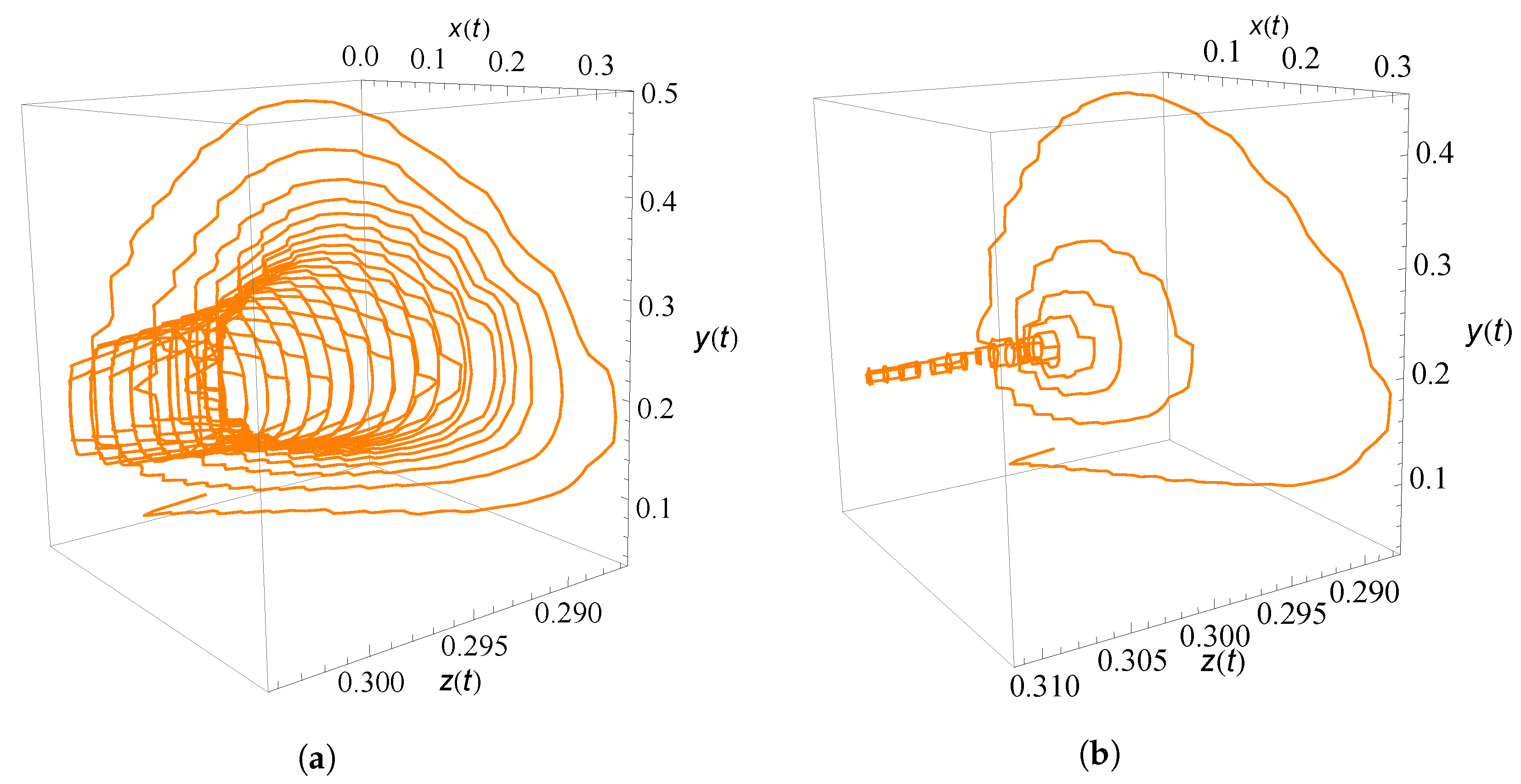
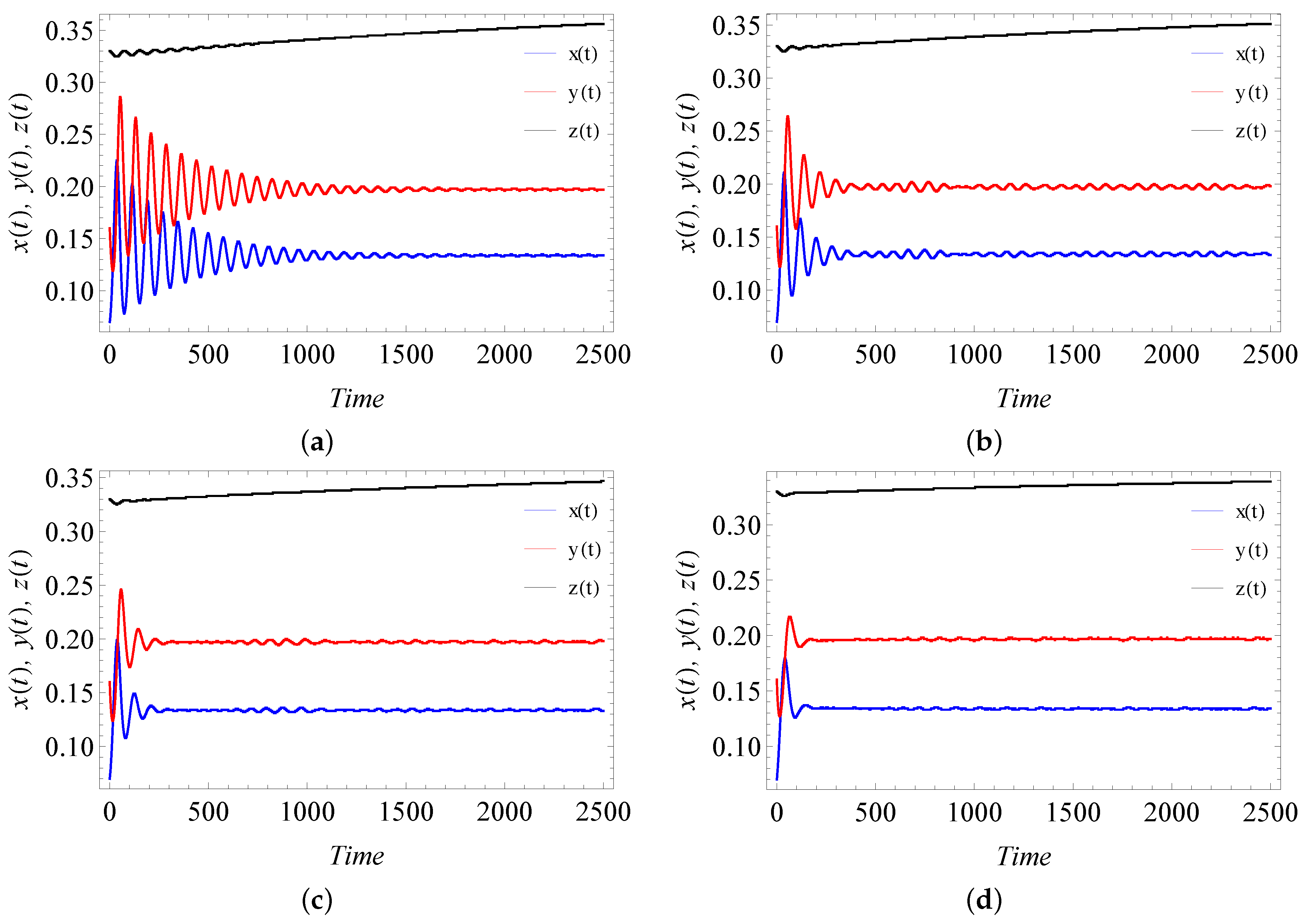
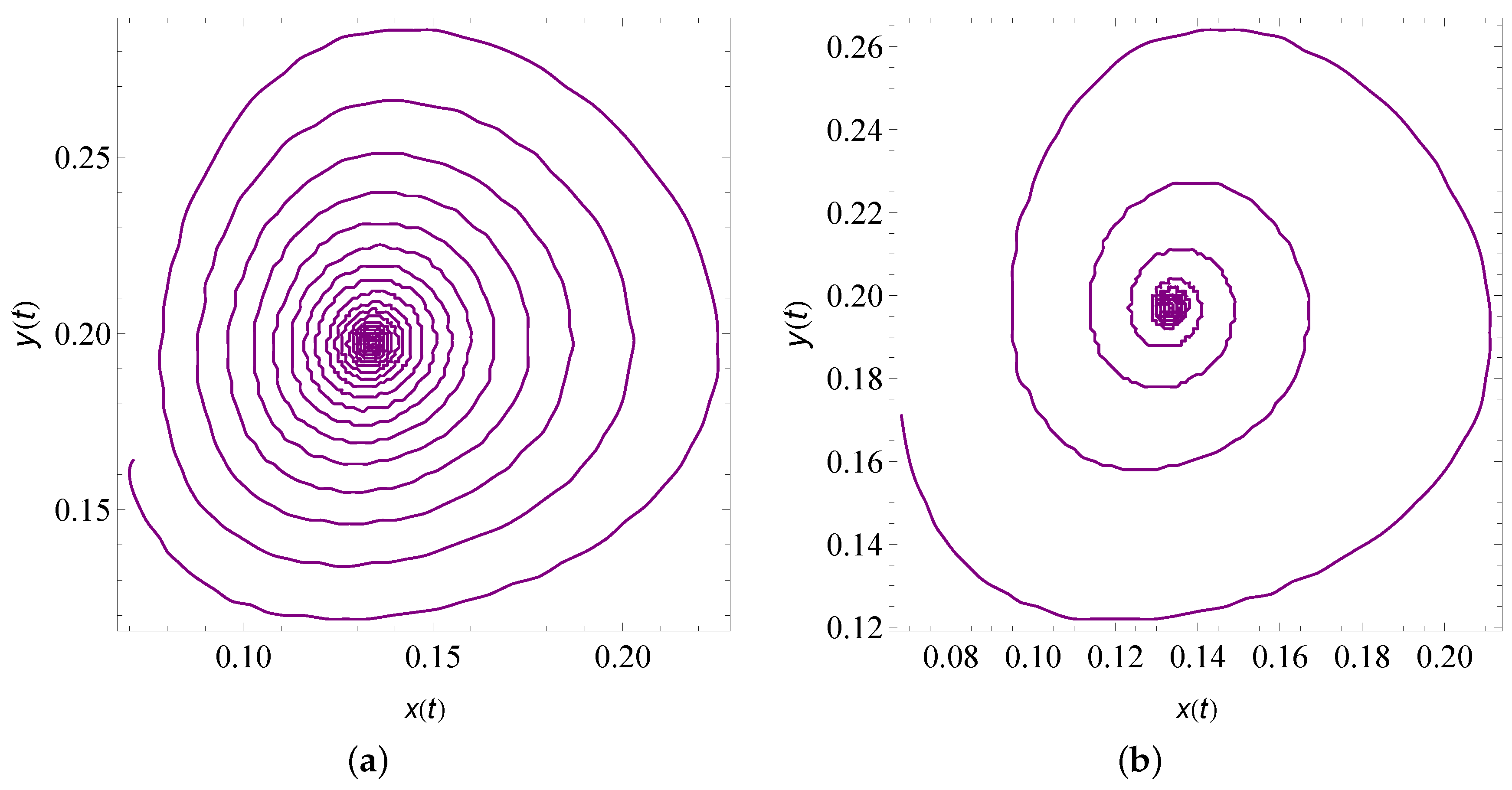
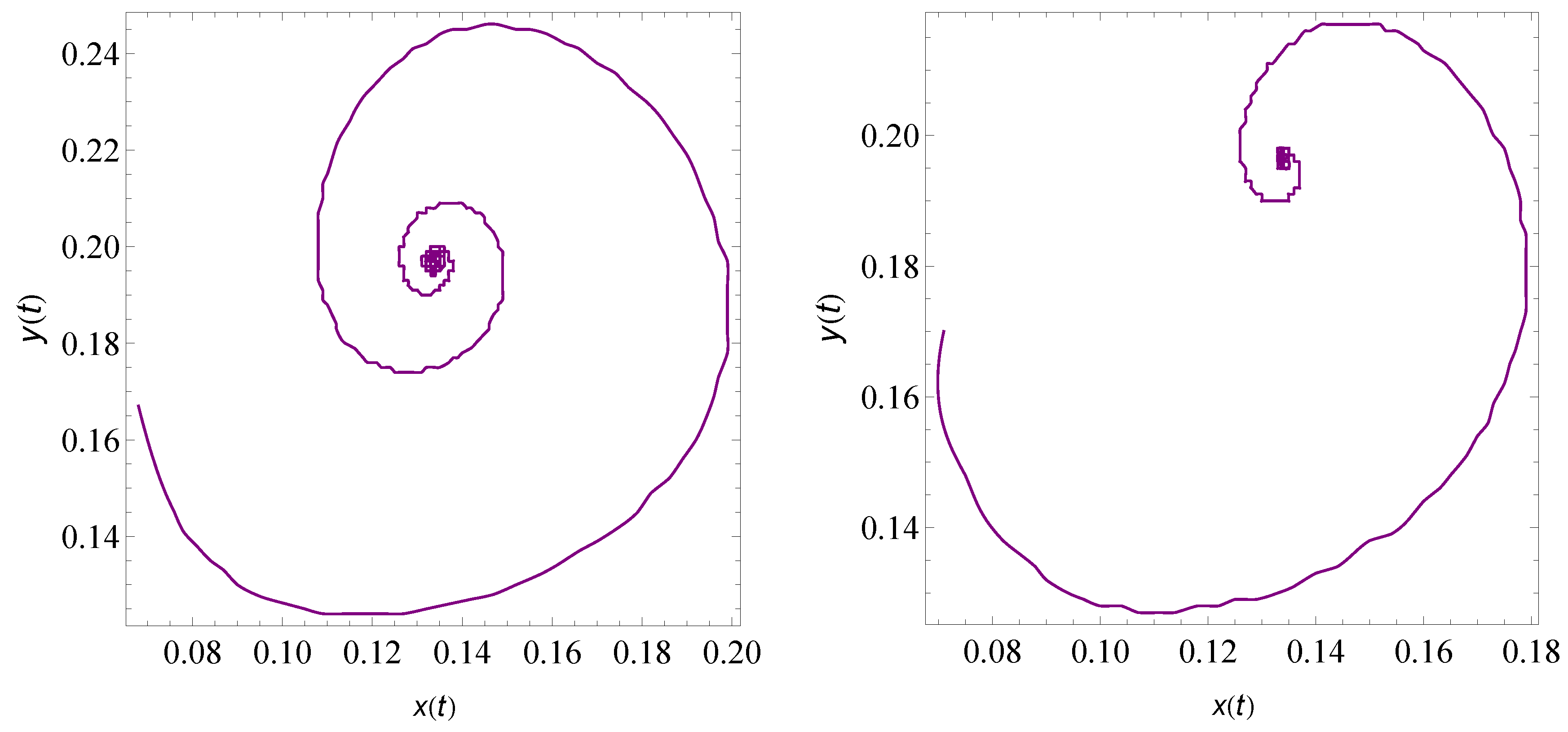
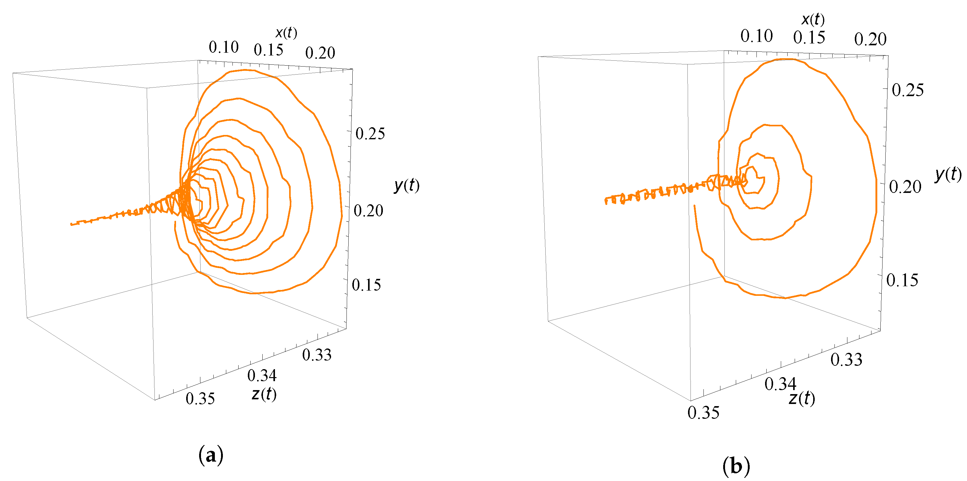
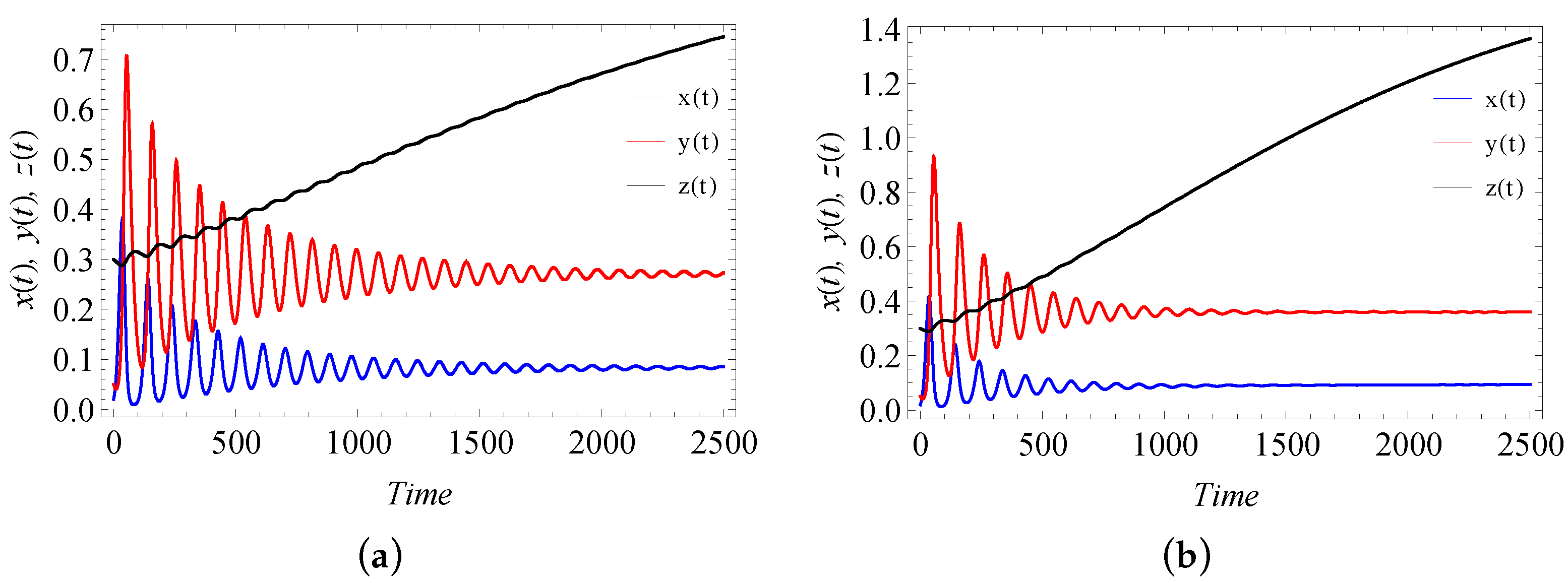
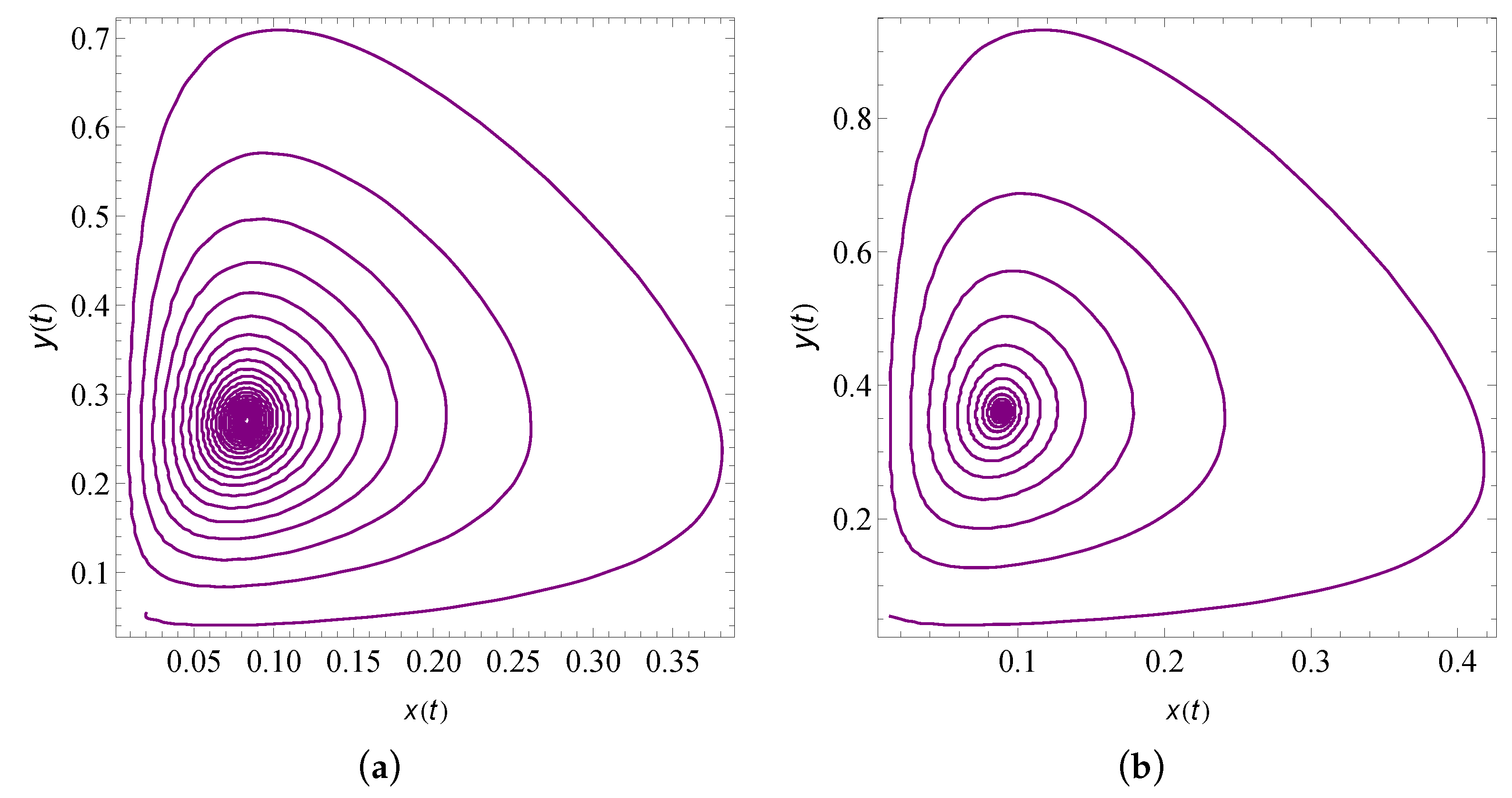
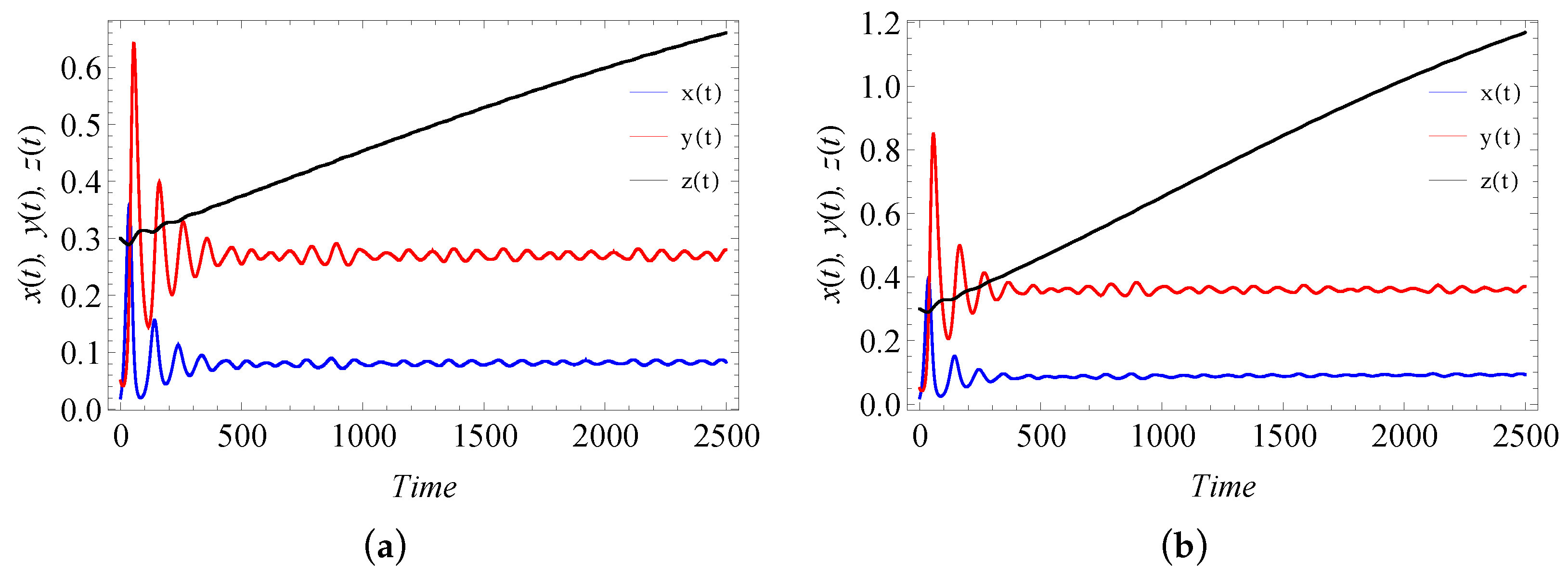
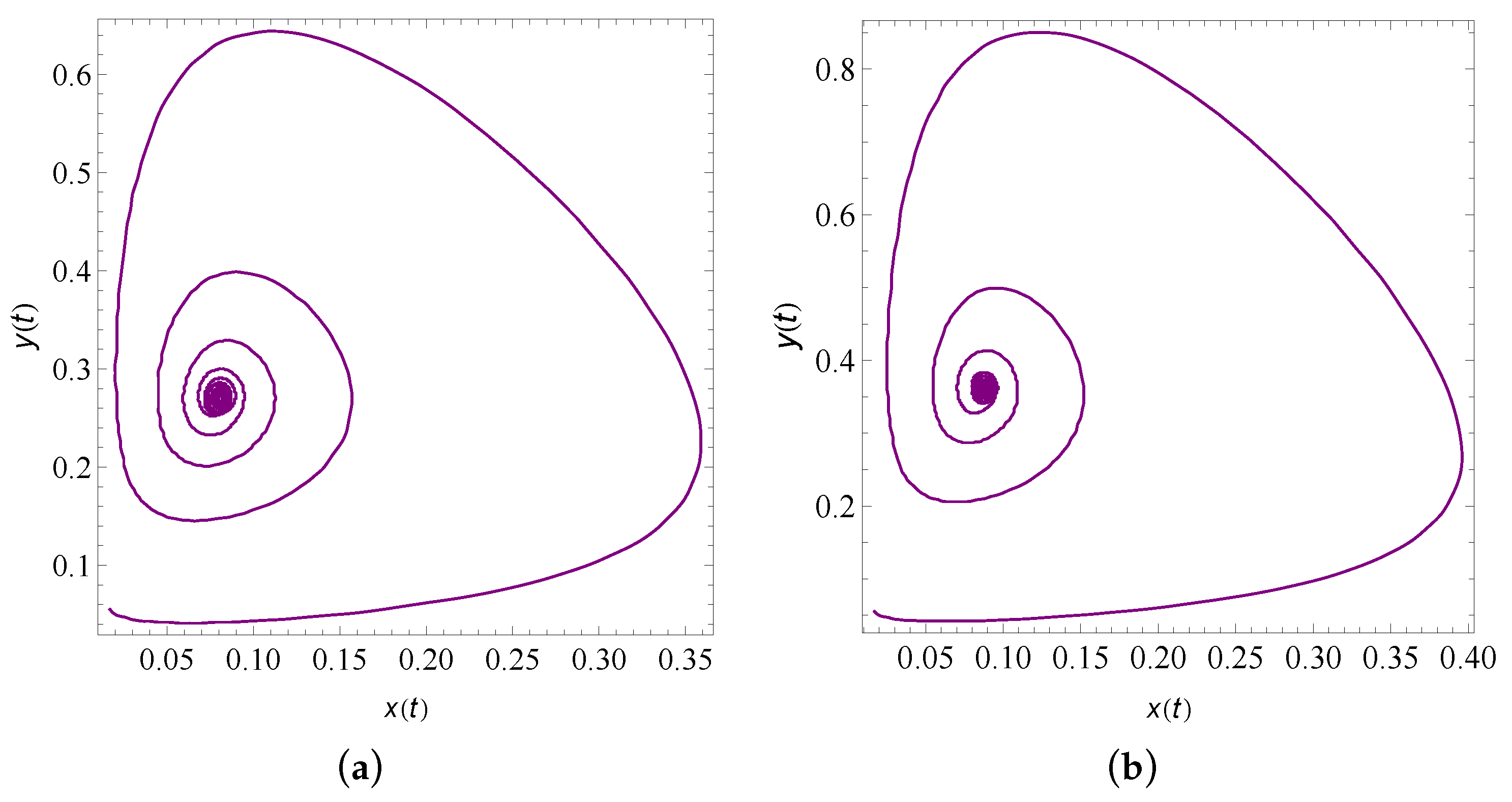
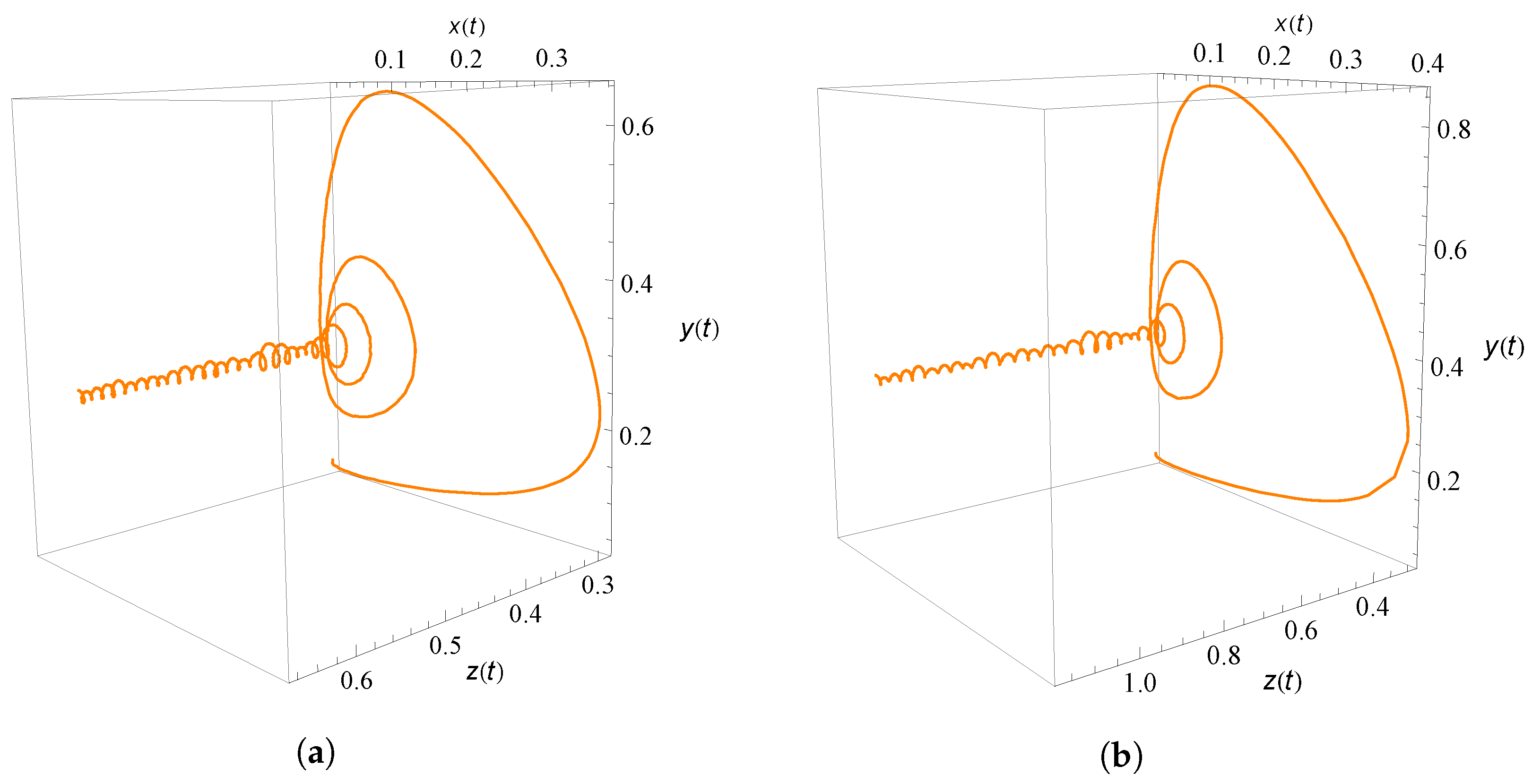
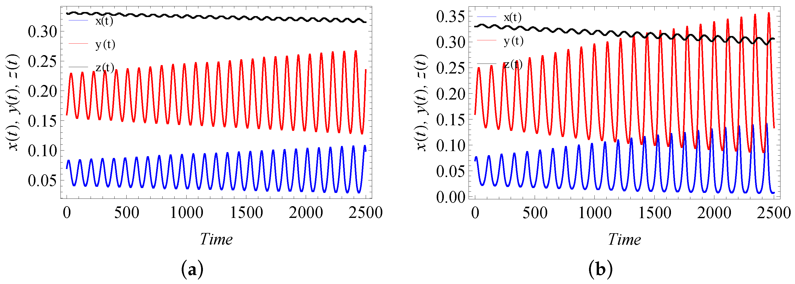
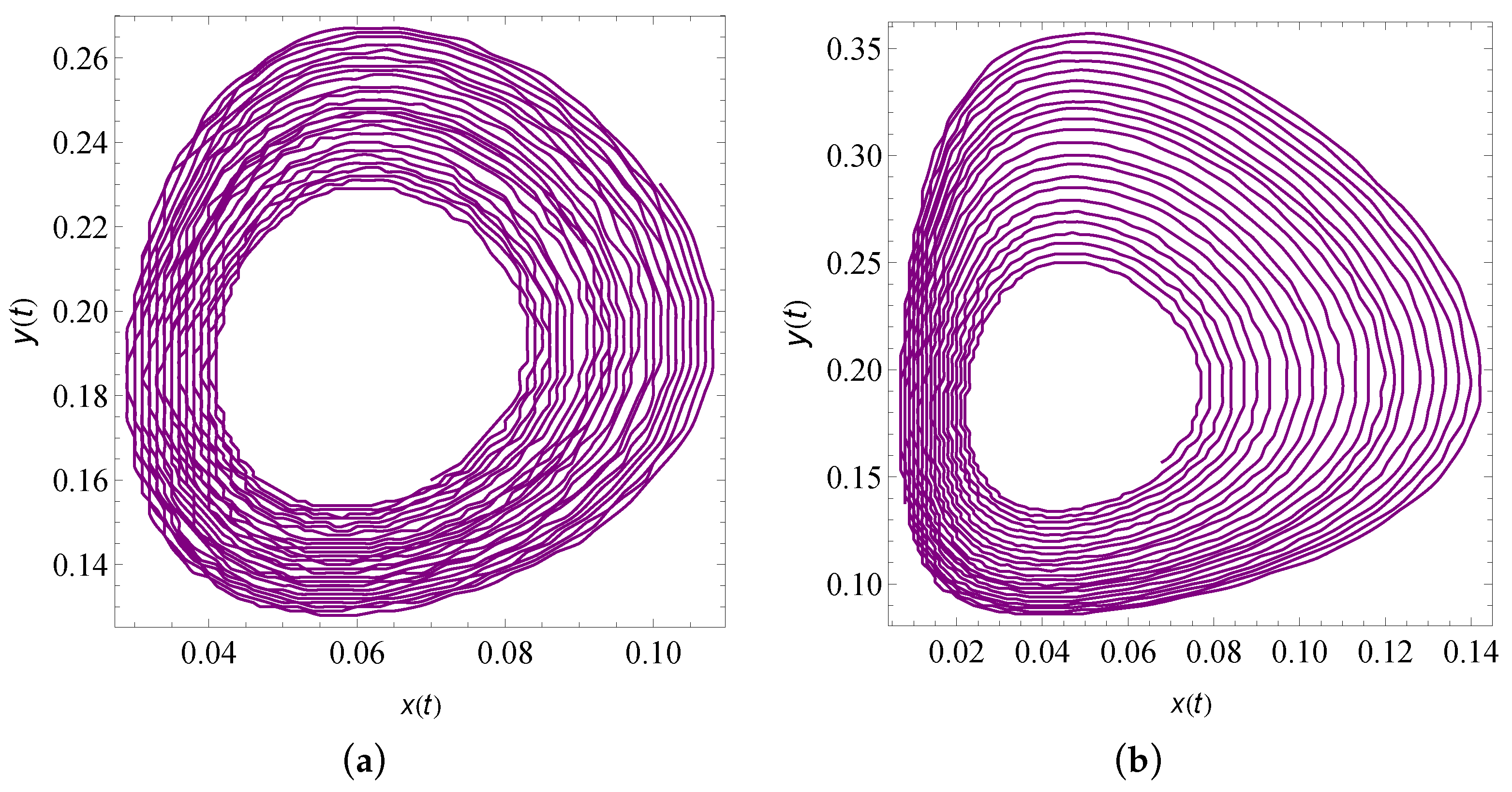
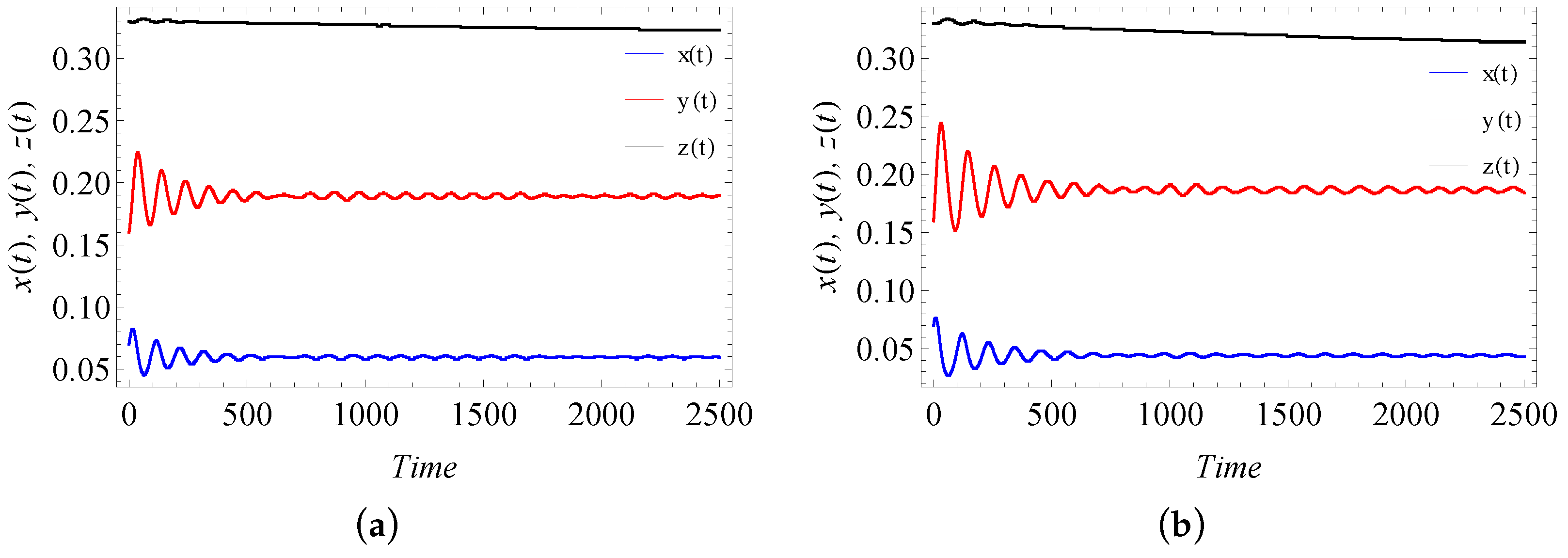
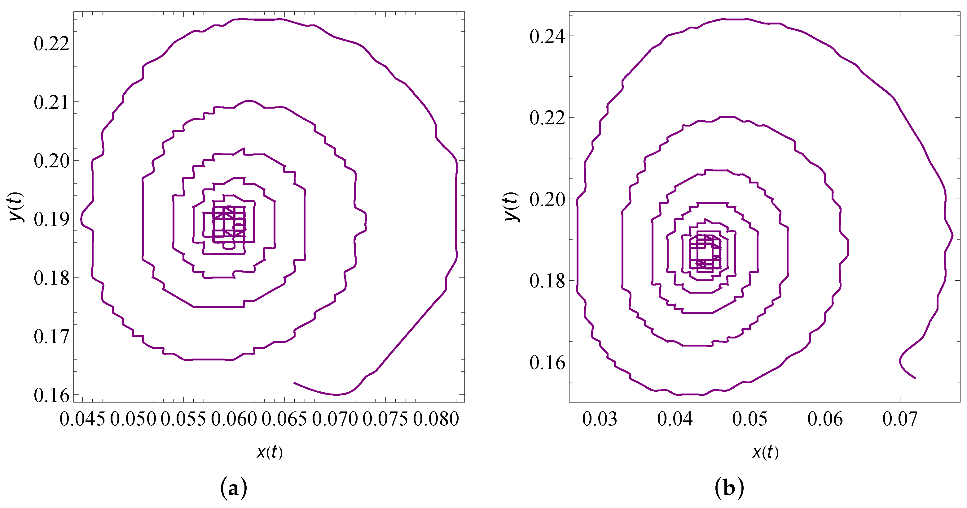
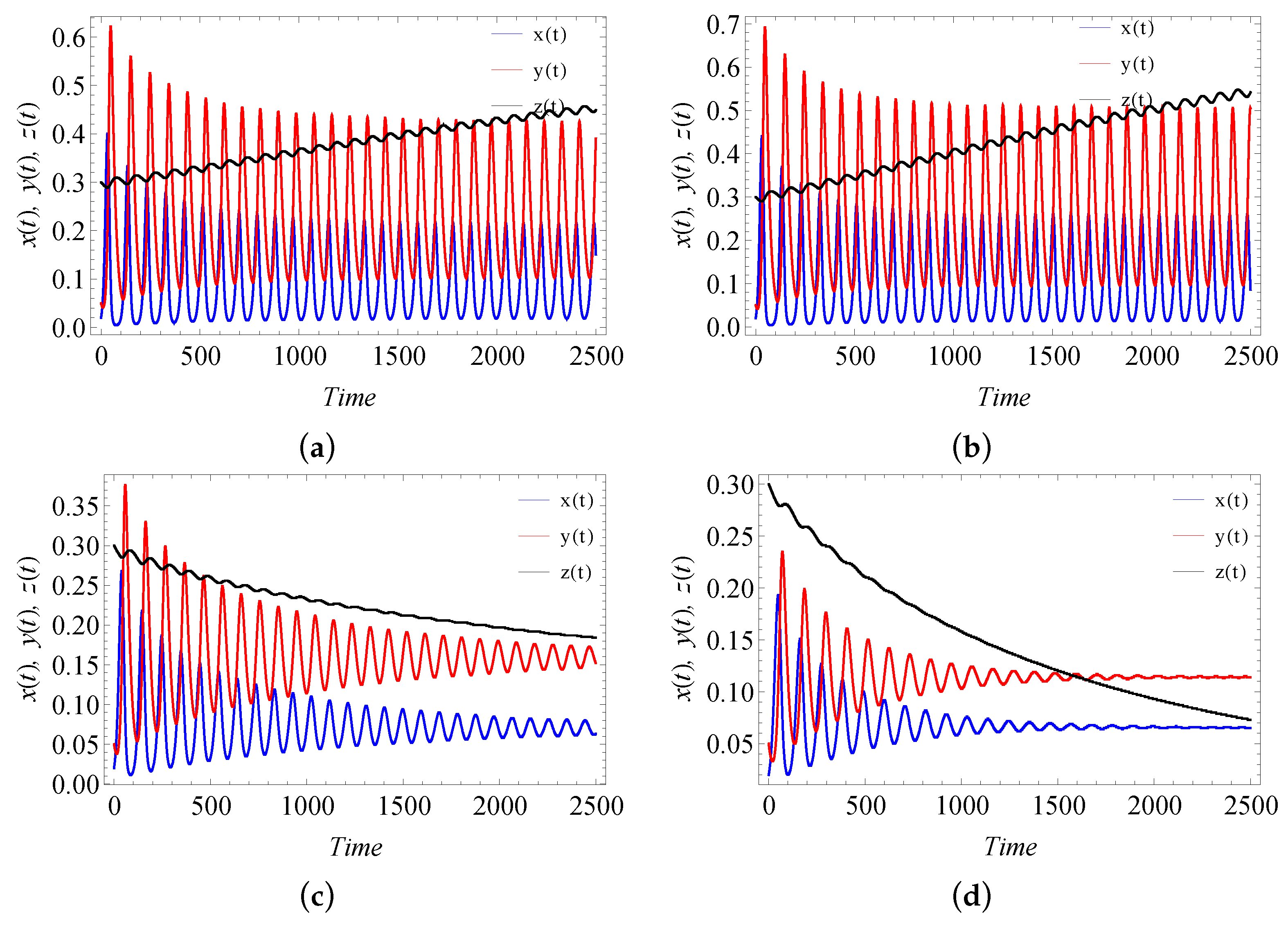
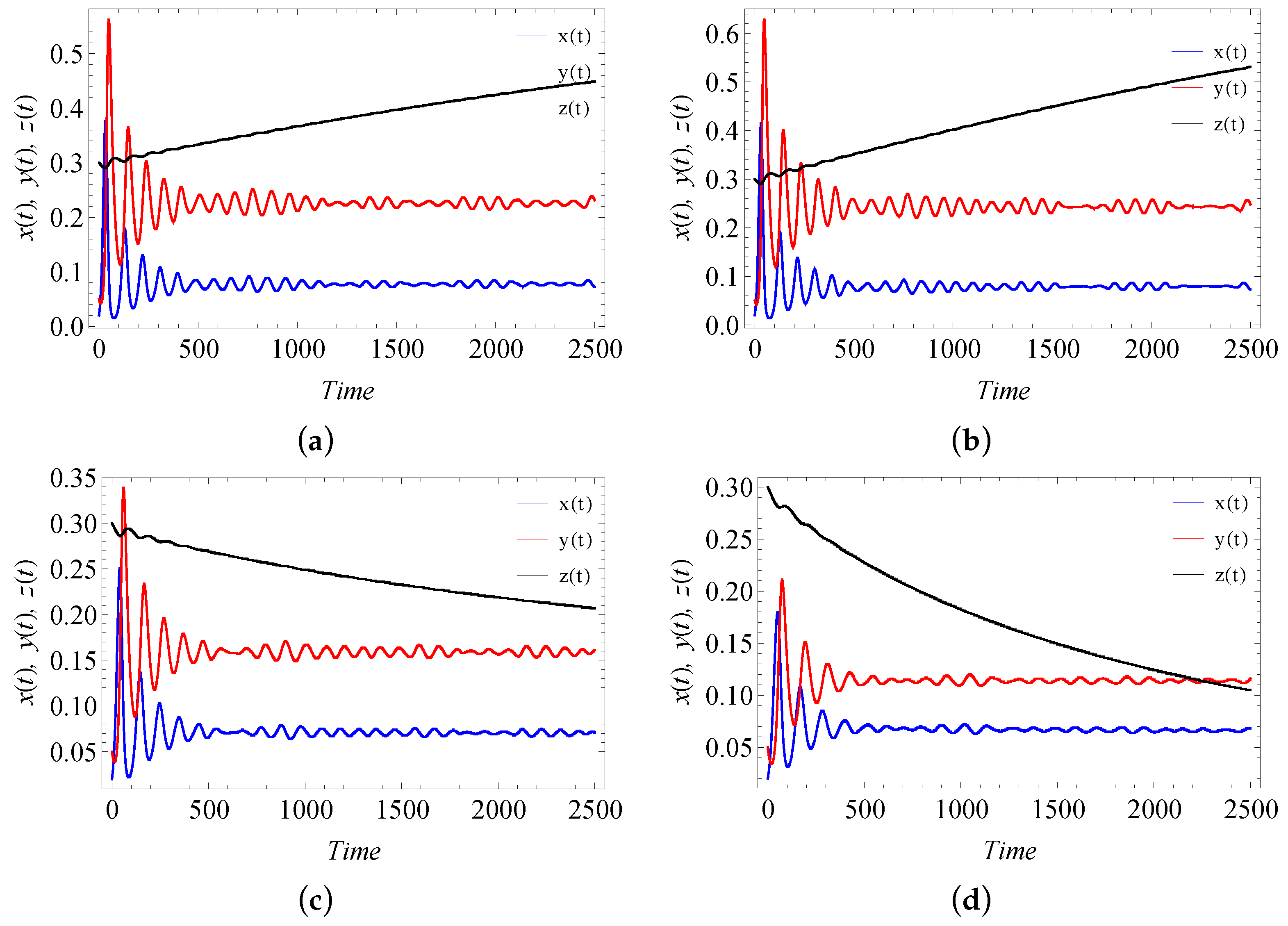
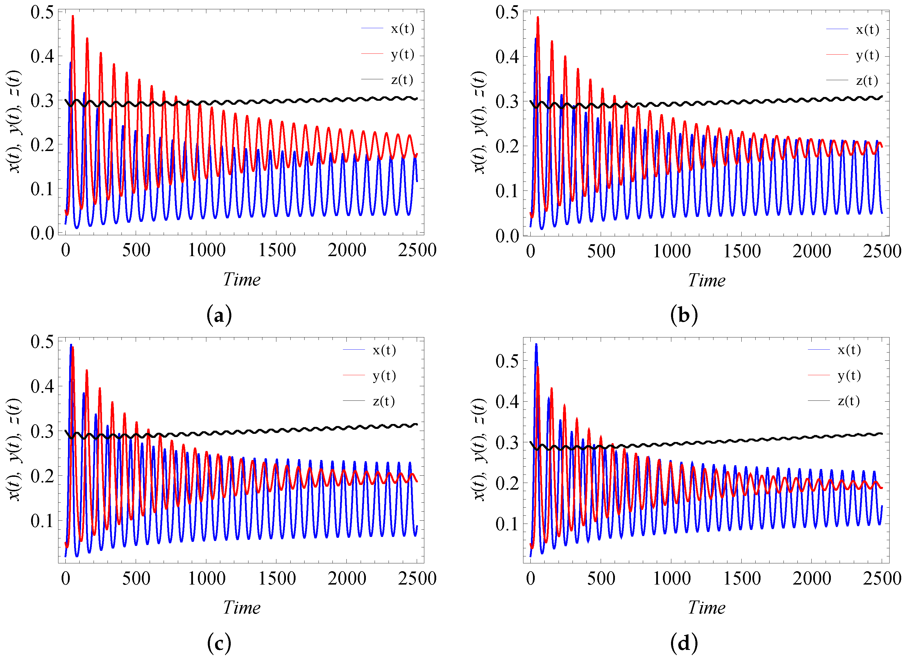
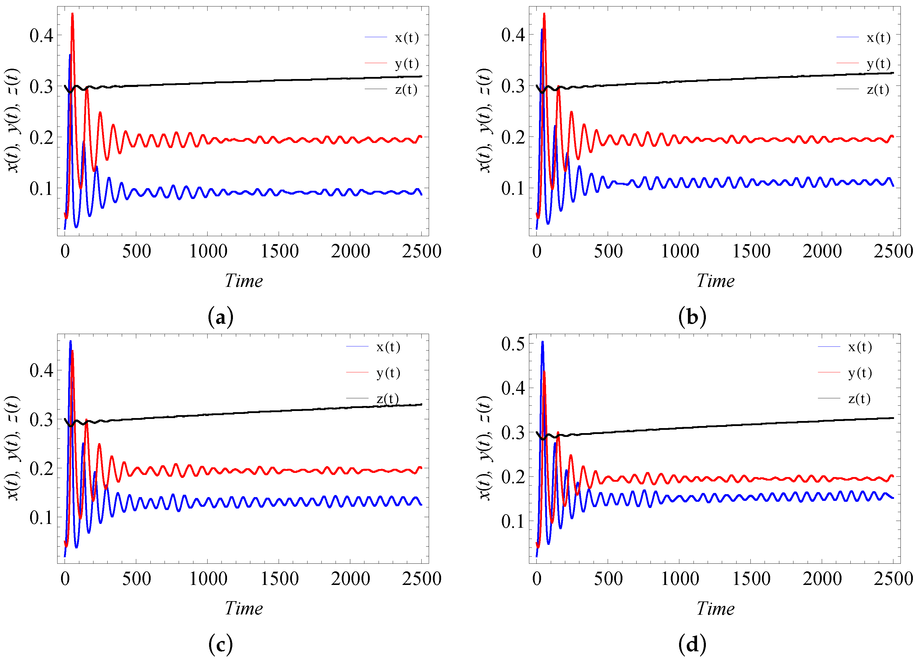
9. Numerical Simulation

In order to discuss the dynamics of the projected fractional order system (8), we have used the generalized Adams–Bashforth–Moulton technique described in Section 7 by considering the parametric values as $r=1$, $c=1$, ${\lambda }_1\in (0.997,1.667)$, $b_0=0.334$, $a_0=0.334$, ${\lambda }_2=1.667$, ${\lambda }_3\in (0.05,0.65)$, $e\in (0.1,0.5)$, $b_1=0.5$, $a_1=0.6$, ${\delta }_1\in (0.15,0.4)$, ${\delta }_2=0.01$ and ${\lambda }_4=0.05$. For Figure 3, Figure 4 and Figure 5, the parametric values are considered as $r=1$, $c=1$, ${\lambda }_1=1.667$, $b_0=0.334$, $a_0=0.334$, ${\lambda }_2=1.667$, ${\lambda }_3=0.05$, $e=0.25$, $b_1=0.5$, $a_1=0.6$, ${\delta }_1=0.2443$, ${\delta }_2=0.01$ and ${\lambda }_4=0.05.$ Unstable behavior of the system (8) can be observed from Figure 3a for the integer order derivative. In Figure 3b–d, it can be noticed that, as the value of the derivative attains fractional value, unstable behavior converges towards spiral stability. The parametric representation presented in Figure 4 and Figure 5 give a very clear view of this observation. It can be inferred that the dynamics of the system (8) can transform from unstable to stable by the amalgamation of fractional derivative.

In Figure 6, Figure 7 and Figure 8, we notice the changing profile of the system (8) from stable spiral to stable focus with the combination of fractional derivative for the set of parameter values $r=1$, $c=1$, ${\lambda }_1=1.667$, $b_0=0.334$, $a_0=0.334$, ${\lambda }_2=1.667$, ${\lambda }_3=0.05$, $e=0.25$, $b_1=0.5$, $a_1=0.6$, ${\delta }_1=0.4$, ${\delta }_2=0.01$ and ${\lambda }_4=0.05$.

In Figure 9, Figure 10, Figure 11, Figure 12, Figure 13 and Figure 14, we have projected the influence of the fractional derivative and the rate of attack on tea plants by pests. We observe that the fractional derivative helps in attaining the stability for the system (8). Again, a notable observation from Figure 9 and Figure 12 is that, as the rate of attack on tea plants by pests decreases, pests population also decreases due to a lack of food and, as a result, tea plants have stable growth.

In Figure 15, Figure 16, Figure 17, Figure 18 and Figure 19, we portray the connection among the three populations with changing death rate ${\delta }_1$ of pests and the fractional derivative. Once again it is established that incorporation of the fractional derivative speeds up the convergence of the solution of the system (8). In Figure 15, we observe that the death rate of the pests impacts the population of pests and the growth of tea plants.

Harvesting the tea plants on time to protect them from pests is a very important phenomenon. Figure 20 and Figure 21 represent the influence of the harvesting parameter e on the three species represented in the system (8). As the amount of harvesting of tea plant increases, the good quality tea leaves are harvested and hence the population of the tea leaves decreases. As a result, the pest population also decreases. Because of the decrease in the pest population, the natural enemies do not get sufficient food and hence their population also decreases.

Figure 22 and Figure 23 represent the effect of the attack rate of natural enemies on the pests’ population in the presence of the fractional derivative. As the attack rate, ${\lambda }_3$, is increased, there is a drop in the population of the pests. Since the pest population decreases, there are fewer attacks from them on the tea leaves. As a result, the population of tea plants increases.

10. Conclusions

In this paper, we have analyzed a three-species food chain model connecting tea plants, pests, and their natural enemies under the influence of the Caputo fractional derivative. We have evaluated the non-negativity of the solutions, conditions for boundedness, and the existence and uniqueness of the projected model. Conditions for the existence and the local stability of the axial, natural, enemy-free and coaxial equilibrium points have been examined. Impacts of pests attack tea plant, pests natural death, tea plant harvesting, and natural enemies attack pests are analyzed in the presence of the fractional derivative. The simulated results of the projected mathematical model reveal that when the order of fractional derivative increases from 0 to 1, system tends to move away from unstable behavior. From the numerical results, it is shown that the numerical method applied in this work is an efficient tool for analyzing the fractional differential equations of a complex nature. In the future, we intend to expand the model to include data fitting and parameter estimates, as well as additional features of the infestation. The three species fractional model can also be adopted with the various functional responses and their dynamical differences compared to the existing models can be observed.

References

1. Biological Control: An Eco-Friendly Way of Pest Management in Tea. 2018. Available online: https://gmsciencein.com/2018/04/23/biological-control-pest-management-tea (accessed on 13 September 2021).
2. Basu Majumder, A.; Bera, B.; Rajan, A. Tea statistics: Global scenario. Inc. J. Tea Sci. 2010, 8, 121–124. [Google Scholar]
3. Cranham, J.E. Tea pests and their control. Annu. Rev. Entomol. 1966, 11, 491–514. [Google Scholar] [CrossRef]
4. Zafar, Z.U.A.; Shah, Z.; Ali, N.; Alzahrani, E.O.; Shutaywi, M. Mathematical and stability Analysis of Fractional Order Model for Spread of Pests in Tea Plants. Fractals 2021, 29, 2150008. [Google Scholar] [CrossRef]
5. Hazarika, L.K.; Bhuyan, M.; Hazarika, B.N. Insect pests of tea and their management. Annu. Rev. Entomol. 2009, 54, 267–284. [Google Scholar] [CrossRef] [Green Version]
6. Hazarika, L.K.; Puzari, K.C.; Wahab, S. Biological control of tea pests. In Biocontrol Potential and Its Exploitation in Sustainable Agriculture; Springer: Boston, MA, USA, 2001; pp. 159–180. [Google Scholar]
7. Maiti, A.; Patra, B.; Samanta, G.P. Sterile insect release method as a control measure of insect pests: A mathematical model. J. Appl. Math. Comput. 2006, 22, 71–86. [Google Scholar] [CrossRef]
8. Pathak, S.; Maiti, A. Microbial pest control: A mathematical model. J. Biol. Syst. 2010, 18, 455–478. [Google Scholar] [CrossRef]
9. Mamun, M.S.A.; Ahmed, M.; Paul, S.K. Integrated approaches in tea pest management for sustainable tea production. In Proceedings of the Workshop on Tea Production Technology Updated, Dhaka, Bangladesh, 24 December 2014; Bangladesh Tea Research Institute, Srimangal, Moulvibazar and Krishi Gobeshona Foundation, BARC Campus: Dhaka, Bangladesh, 2014; Volume 24, pp. 18–32. [Google Scholar]
10. Muraleedharan, N. Pest control in Asia. In Tea; Springer: Dordrecht, The Netherlands, 1992; pp. 375–412. [Google Scholar]
11. Liu, S.S.; Rao, A.; Vinson, S.B. Biological control in china: Past, present and future—An introduction to this special issue. Biol. Control 2014, 68, 1–5. [Google Scholar] [CrossRef]
12. Landis, D.A.; Orr, D.B. Biological Control: Approaches and Applications. 1996. Available online: https://ipmworld.umn.edu/landis (accessed on 13 September 2021).
13. The Advantages and Disadvantages of Pesticides. Available online: https://www.chefsbest.com/advantages-disadvantages-pesticides/ (accessed on 13 September 2021).
14. Aktar, M.W.; Sengupta, D.; Chowdhury, A. Impact of pesticides use in agriculture: Their benefits and hazards. Interdiscip. Toxicol. 2009, 2, 1–12. [Google Scholar] [CrossRef] [Green Version]
15. Wahab, S. Tea pests and their management with bio-pesticides. Int. J. Tea Sci. 2004, 3, 1–10. [Google Scholar]
16. Nakai, M. Biological control of tortricidae in tea fields in Japan using insect viruses and parasitoids. Virol. Sin. 2009, 24, 323–332. [Google Scholar] [CrossRef]
17. Stoner, K. Approaches to the Biological Control of Insect Pests. Available online: https://portal.ct.gov/CAES/Fact-Sheets/Entomology/Approaches-to-the-Biological-Control-of-Insect-Pests (accessed on 14 September 2021).
18. Hastings, A.; Powell, T. Chaos in a three-species food chain. Ecology 1991, 72, 896–903. [Google Scholar] [CrossRef]
19. Panja, P.; Mondal, S.K.; Jana, D.K. Effects of toxicants on Phytoplankton-Zooplankton-Fish dynamics and harvesting. Chaos Solitons Fractals 2017, 104, 389–399. [Google Scholar] [CrossRef]
20. Panja, P. Stability and dynamics of a fractional-order three-species predator–prey model. Theory Biosci. 2019, 138, 251–259. [Google Scholar] [CrossRef]
21. Baishya, C.; Veeresha, P. Laguerre polynomial-based operational matrix of integration for solving fractional differential equations with non-singular kernel. Proc. R. Soc. A 2021, 477, 20210438. [Google Scholar] [CrossRef]
22. Sun, H.; Zhang, Y.; Baleanu, D.; Chen, W.; Chen, Y. A new collection of real world applications of fractional calculus in science and engineering. Commun. Nonlinear Sci. Numer. Simul. 2018, 64, 213–231. [Google Scholar] [CrossRef]
23. Baishya, C. An operational matrix based on the Independence polynomial of a complete bipartite graph for the Caputo fractional derivative. SeMA J. 2021. [Google Scholar] [CrossRef]
24. Akinyemi, L.; Iyiola, O.S. Exact and approximate solutions of time-fractional models arising from physics via Shehu transform. Math. Methods Appl. Sci. 2020, 43, 7442–7464. [Google Scholar] [CrossRef]
25. Baishya, C.; Achar, S.J.; Veeresha, P.; Prakasha, D.G. Dynamics of a fractional epidemiological model with disease infection in both the populations. Chaos 2021, 31, 043130. [Google Scholar] [CrossRef]
26. Owusu-Mensah, I.; Akinyemi, L.; Oduro, B.; Iyiola, O.S. A fractional order approach to modeling and simulations of the novel COVID-19. Adv. Differ. Equs. 2020, 2020, 683. [Google Scholar] [CrossRef]
27. Veeresha, P.; Baleanu, D. A unifying computational framework for fractional Gross-Pitaevskii equations. Phys. Scr. 2021, 96, 125010. [Google Scholar]
28. Iyiola, O.; Oduro, B.; Akinyemi, L. Analysis and solutions of generalized Chagas vectors re-infestation model of fractional order type. Chaos Solitons Fractals 2021, 145, 110797. [Google Scholar] [CrossRef]
29. Bagley, R.L.; Torvik, P.J. A theoretical basis for the application of fractional calculus to viscoelasticity. J. Rheol. 1983, 27, 201–210. [Google Scholar] [CrossRef]
30. Veeresha, P.; Akinyemi, L.; Oluwasegun, K.; Şenol, M.; Oduro, B. Numerical surfaces of fractional Zika virus model with diffusion effect of mosquito-borne and sexually transmitted disease. In Mathematical Methods in the Applied Sciences; Wiley: Hoboken, NJ, USA, 2021. [Google Scholar]
31. Sokolov, I.M. Models of anomalous diffusion in crowded environments. Soft Matter 2012, 8, 9043–9052. [Google Scholar] [CrossRef]
32. Metzler, R.; Jeon, J.H.; Cherstvy, A.G.; Barkai, E. Anomalous diffusion models and their properties: Non-stationarity, non-ergodicity, and ageing at the centenary of single particle tracking. Phys. Chem. Chem. Phys. 2014, 16, 24128–24164. [Google Scholar] [CrossRef] [Green Version]
33. Kepten, E.; Weron, A.; Sikora, G.; Burnecki, K.; Garini, Y. Guidelines for the fitting of anomalous diffusion mean square displacement graphs from single particle tracking experiments. PLoS ONE 2015, 10, e0117722. [Google Scholar] [CrossRef] [PubMed]
34. Kumar, S.; Kumar, R.; Cattani, C.; Samet, B. Chaotic behaviour of fractional predator-prey dynamical system. Chaos Solitons Fractals 2020, 135, 109811. [Google Scholar] [CrossRef]
35. Huang, C.; Li, H.; Cao, J. A novel strategy of bifurcation control for a delayed fractional predator-prey model. Appl. Math. Comput. 2019, 347, 808–838. [Google Scholar] [CrossRef]
36. Ghanbari, B.; Kumar, D. Numerical solution of predator-prey model with Beddington-DeAngelis functional response and fractional derivatives with Mittag-Leffler kernel. Chaos Interdiscip. J. Nonlinear Sci. 2019, 29, 063103. [Google Scholar] [CrossRef] [PubMed]
37. Kumar, S.; Kumar, A.; Jleli, M. A numerical analysis for fractional model of the spread of pests in tea plants. In Numerical Methods for Partial Differential Equations; Wiley: Hoboken, NJ, USA, 2020. [Google Scholar]
38. Lopes, A.M.; Machado, J.T. Fractional order models of leaves. J. Vib. Control 2014, 20, 998–1008. [Google Scholar] [CrossRef] [Green Version]
39. El-Shahed, M.; Ahmed, A.M.; Abdelstar, I.M. A fractional-order Model for the spread of Pests in tea plants. Adv. Anal. 2016, 1, 68–79. [Google Scholar] [CrossRef]
40. Podlubny, I. Fractional Differential Equations: An Introduction to Fractional Derivatives, Fractional Differential Equations, to Methods of Their Solution and Some of Their Applications; Elsevier: Amsterdam, The Netherlands, 1998. [Google Scholar]
41. Wang, B.; Chen, L.Q. Asymptotic stability analysis with numerical confirmation of an axially accelerating beam constituted by the standard linear solid model. J. Sound Vib. 2009, 328, 456–466. [Google Scholar] [CrossRef]
42. Li, H.L.; Zhang, L.; Hu, C.; Jiang, Y.L.; Teng, Z. Dynamical analysis of a fractional-order predator-prey model incorporating a prey refuge. J. Appl. Math. Comput. 2017, 54, 435–449. [Google Scholar] [CrossRef]
43. Agarwal, M.; Pathak, R. Harvesting, Hopf bifurcation and chaos in three species food chain model with Beddington-DeAngelis type functional response. J. Glob. Res. Math. Arch. 2013, 1, 49–62. [Google Scholar]
44. Diethelm, K. An algorithm for the numerical solution of differential equations of fractional order. Electron. Trans. Numer. Anal. 1997, 5, 1–6. [Google Scholar]
45. Diethelm, K.; Ford, N.J. Analysis of fractional differential equations. J. Math. Anal. Appl. 2002, 265, 229–248. [Google Scholar] [CrossRef] [Green Version]
46. Diethelm, K.; Ford, N.J.; Freed, A.D. A predictor-corrector approach for the numerical solution of fractional differential equations. Nonlinear Dyn. 2002, 29, 3–22. [Google Scholar] [CrossRef]
Figure 1. Tea pests and damages [1,5].
Fractalfract 06 00001 g001
Figure 2. Natural enemies of (a) Looper, (b) Aphid, (c) Red spider [1,5].
Fractalfract 06 00001 g002
Figure 3. Unstable to stable profile of the system (8) for (a) α = 1 , (b) α = 0.95 , (c) α = 0.9 , and (d) α = 0.8 .
Fractalfract 06 00001 g003
Figure 4. Two dimensional (2D) view of unstable to stable profile of the system (8) for (a) α = 1 , (b) α = 0.95 , (c) α = 0.9 , and (d) α = 0.8 .
Fractalfract 06 00001 g004
Figure 5. Three dimensional (3D) view of convergence from unstable to stable solution of the system (8) for (a) α = 1 and (b) α = 0.95 .
Fractalfract 06 00001 g005
Figure 6. Profile of the system (8) from stable spiral to stable focus for (a) α = 1 , (b) α = 0.95 , (c) α = 0.9 , and (d) α = 0.8 .
Fractalfract 06 00001 g006
Figure 7. Profile of the system (8) from stable spiral to stable focus for (a) α = 1 , (b) α = 0.95 , (c) α = 0.9 , and (d) α = 0.8 .
Fractalfract 06 00001 g007aFractalfract 06 00001 g007b
Figure 8. Profile of the system (8) for (a) α = 1 and (b) α = 0.95 .
Fractalfract 06 00001 g008
Figure 9. Influence of the rate of attack on tea plants by pests (a) λ 1 = 1.251 and (b) λ 1 = 0.997 for α = 1 .
Fractalfract 06 00001 g009
Figure 10. Influence of the rate of attack on tea plants by pests (a) λ 1 = 1.251 and (b) λ 1 = 0.997 for α = 1 .
Fractalfract 06 00001 g010
Figure 11. Influence of the rate of attack on tea plants by pests (a) λ 1 = 1.251 and (b) λ 1 = 0.997 for α = 1 .
Fractalfract 06 00001 g011
Figure 12. Influence of the rate of attack on tea plants by pests (a) λ 1 = 1.251 and (b) λ 1 = 0.997 for α = 0.95 .
Fractalfract 06 00001 g012
Figure 13. Influence of the rate of attack on tea plants by pests (a) λ 1 = 1.251 and (b) λ 1 = 0.997 for α = 0.95 .
Fractalfract 06 00001 g013
Figure 14. Influence of the rate of attack on tea plants by pests (a) λ 1 = 1.251 and (b) λ 1 = 0.997 for α = 0.95 .
Fractalfract 06 00001 g014
Figure 15. Influence of death rate δ 1 of pests (a) δ 1 = 0.2 and (b) δ 1 = 0.15 for α = 1 .
Fractalfract 06 00001 g015
Figure 16. Influence of death rate δ 1 of pests (a) δ 1 = 0.2 and (b) δ 1 = 0.15 for α = 1 .
Fractalfract 06 00001 g016
Figure 17. Influence of death rate δ 1 of pests (a) δ 1 = 0.2 and (b) δ 1 = 0.15 for α = 1 .
Fractalfract 06 00001 g017
Figure 18. Influence of death rate δ 1 of pests (a) δ 1 = 0.2 and (b) δ 1 = 0.15 for α = 0.95 .
Fractalfract 06 00001 g018
Figure 19. Influence of death rate δ 1 of pests (a) δ 1 = 0.2 and (b) δ 1 = 0.15 for α = 0.95 .
Fractalfract 06 00001 g019
Figure 20. Effect of tea plant harvesting (a) e = 0.1 , (b) e = 0.15 , (c) e = 0.35 , and (d) e = 0.5 for α = 1 .
Fractalfract 06 00001 g020
Figure 21. Effect of tea plant harvesting (a) e = 0.1 , (b) e = 0.15 , (c) e = 0.35 , and (d) e = 0.5 for α = 0.9 .
Fractalfract 06 00001 g021
Figure 22. Effect of the attack rate of natural enemies (a) λ 3 = 0.2 , (b) λ 3 = 0.35 , (c) λ 3 = 0.5 , and (d) λ 3 = 0.65 for α = 1 .
Fractalfract 06 00001 g022
Figure 23. Effect of the attack rate of natural enemies (a) λ 3 = 0.2 , (b) λ 3 = 0.35 , (c) λ 3 = 0.5 , and (d) λ 3 = 0.65 for α = 0.9 .
Fractalfract 06 00001 g023
Publisher’s Note: MDPI stays neutral with regard to jurisdictional claims in published maps and institutional affiliations.