Article

Between 2D and 3D: Studying Structural Complexity of Urban Fabric Using Voxels and LiDAR-Derived DSMs

1
School of Architecture and Urban Design, RMIT University, Melbourne 3000, Australia
2
Landscape Architecture and Spatial Planning Group, Wageningen University and Research, 6700 HB Wageningen, The Netherlands
3
School of Landscape Architecture, Lincoln University, Lincoln 7647, New Zealand
*
Author to whom correspondence should be addressed.
Fractal Fract. 2021, 5(4), 227; https://doi.org/10.3390/fractalfract5040227
Submission received: 23 September 2021 / Revised: 12 November 2021 / Accepted: 15 November 2021 / Published: 17 November 2021

Abstract

:
Cities are complex systems and their physical forms are the manifestation of cultural, social and economic processes shaped by the geometry of natural and man-made elements. Digital Surface Models (DSM) using LiDAR provide an efficient volumetric transformation of urban fabric including all built and natural elements which allows the study of urban complexity through the lens of fractal dimension (D). Founded on the “box-counting” method, we reveal a voxelization technique developed in GIS (Geographic Information System) to estimate D values of ten DSM samples across central Melbourne. Estimated D values of surface models (between 2 and 3) provide a measure to interpret the structural complexity of different urban characters defined by the pattern of developments and densities. The correlations between D values with other DSM properties such as elevation, volume, solar radiation and surface roughness, showed a strong relationship between DSM volume and mean elevation. Lower strength correlations were recorded with solar radiation and surface roughness. The proposed method provides opportunities for fractal research to study pressing issues in complex urban environments such as declining physical fitness, mental health and urban biodiversity.

1. Introduction

Urban environments are complex systems whose physical forms are the manifestation of cultural, social and economic processes shaped by the geometry of the natural and man-made world [1]. The complexity of urban forms, similar to that of natural systems, cannot be fully determined by Euclidean geometry. However, the concept of a fractal dimension has previously successfully been used to describe this complexity [2]. Indeed, the geometric order created from self-similarity, which is a core characteristic of fractals, can be measured to describe these complex forms [3]. Therefore, fractal geometry is a useful mathematical concept for the spatial analysis of cities, enabling the assemblage of a bigger picture of complex forms that might be of use to social scientists, geographers, economists, planners, engineers and designers.
The discovery of fractal geometry by Mandelbrot [4] changed the appreciation of complex forms and patterns available in nature. Fractal objects are self-similar through an assemblage of rescaled copies of themselves and when rescaling are either anisotropic or dependent on a direction [5]. These objects or forms are too complex to be described in Euclidean space by topological Cartesian dimensions (1D, 2D or 3D). Instead, they can be characterised by a value of fractal dimension, a statistical concept summarising the degree of self-similarity. A higher fractal dimension indicates higher complexity or irregularity than a lower fractal dimension. Therefore, urban environments, as complex geometries resulting from interactions of man-made and natural elements occurring at macro and micro levels, can be successfully analysed.

1.1. Fractal Analysis of Built Environments

The use of fractal geometry in urban studies mainly developed in the 1990s [6]. Indeed, previous studies have shown that cities can be conceptualised as fractals at several, nested and interrelated, scales. In macro-scale analysis, various researchers have used the concept of fractal dimension to analyse urban environments and have articulated the importance of this measure in town planning [1,7,8,9]. For example, Batty and Longley [1] developed a method for adapting measurements of fractal dimensions to analyse the visual growth patterns of large-scale urban settlements. Batty [8] explored the topological properties of multiple complex networks of urban cities. Cardillo et al. [9] analysed the fractal dimension of street networks of 20 different cities in 1-square-mile samples. Other researchers have used fractal geometry to analyse different qualities and elements of urban environments [2,10,11]. Chalup et al. [12], Chalup and Ostwald [13] and Tucker et al. [14] used the concept of fractal dimension as an anthropocentric bio-cybernetic approach to analyse the built environment, by measuring the fractal dimensions of city skylines and identifying different types of cityscapes. Cooper and Oskrochi [10] applied the box-counting method to calculate the fractal dimension of 26 streetscapes to identify any relationship between visual variety in urban design with fractal dimension. They found a significant correlation between D and subjective judgements. Cooper [15] used the fractal assessment of street skylines to assess the character of urban areas in relation to their physical characteristics. He found that streets with higher levels of vegetation, undulating rooflines and narrow buildings would yield higher D values. Following this, Cooper [16] assessed the fractal dimension of street edges by tracing building frontages using 1:2000 plan outlines and derived a typology of street characteristics based on these values. He found that streets would exhibit different D values in relation to the variety of building type and size, with a higher D being a sign of greater variety.
Values of fractal dimension have been found to differentiate between different types of urban characters. For example, looking at Brussels, values of D were significantly different between the city centre and the periphery, illustrating the increase in compactness of urban clusters as the distance to the centre decreases [6]. However, the fractal dimension seems to capture a different aspect of urban morphology than density alone. Indeed, whereas density is represented as mass per surface, D refers to the spatial distribution of this mass [6]. Qin et al. [17] developed a three-dimensional box-counting method to estimate the fractal dimension of urban form change using remote sensing images. Chen [18] explained cities as pre-fractals rather than real fractals as they have a limited hierarchy, indicating a fractal-like geometric form.
At smaller scales, Bovill [19] in Fractal Geometry in Architecture and Design approximate the fractal dimension of built forms. Following this, numerous studies have measured the fractal dimension of architecture [2,10,14,20,21]. Sala [20] applied Bovill’s method to Frank Lloyd Wright’s Robie house. Architectural works of multiple well-known architects such as Le Corbusier, Frank Lloyd Wright, Eileen Gray, Peter Eisenman, Glenn Murcutt and Kazuyo Sejima were analysed using fractal dimension [2,22,23]. Stamps [11] and Ostwald and Vaughan [2] also compared nature and architecture using the fractal dimension to analyse relationships between architecture and its setting.
The application of fractal dimension in built environments is a vibrant area of research. New approaches to estimating fractal dimension and complexity in other fields such as medical [24], geospatial [25] and material science [26,27,28] are inspiring for application in built environments. This requires linking and interpreting measurements to the established concepts in design and planning.

1.2. Structural Complexity and Application

Geometric complexity is a familiar concept to researcher’s in-built environments whilst structural complexity may be a new concept. According to the Oxford Dictionary [29], geometry refers to the spatial attributes of an object, while structure refers to a cohesive whole made up of distinct parts. Structural complexity has been widely studied by ecologists, particularly in studying coral reefs by linking biodiversity to the carrying capacity of habitats [30,31]. Structural complexity is defined as the physical three-dimensional structure of an ecosystem, which reflects the heterogeneity and irregularity levels of structural elements. Although it appears similar to the geometrical complexity, it is applied to an assemblage of elements rather than a single object. A strong correlation has been identified between the structural complexity of coral reefs and species richness. Fractal dimension has been used in studying this diversity in terrestrial and marine environments [31].
The structure of urban environments forms by roads, buildings, streetscape plantings, footpaths, signage, lighting, and many other assembled elements. The combination of these elements in various sizes shapes the urban fabric or physical form of urbanised areas. The collective complexity resulting from the combination of these elements can be studied using fractal dimensions, similar to coral reef ecosystems. The heterogeneity and irregularity of similar urban systems, and their impact on the health of inhabitants, highlights interesting possibilities for research in urban environments. The numerical characterisation of different types of urban characters in a 3-dimensional form would allow the identification of relationships between changing urban environments and human health and well being [32]. Although urban areas often have better health outcomes than rural areas, such outcomes can be eroded by a deteriorating amenity and biodiversity of urban environments [33].

1.3. Tangibility of Urban Environments

Amenity is considered to be a difficult concept to define in planning discourses [33]. The concept of amenity as the pleasantness and attractiveness of urban environments and their effectiveness in utilizing environmental and physical needs are some of the key considerations for city planners and designers. Amenity is considered as a quality that includes tangible and intangible aspects and is like an umbrella that covers a broad range of planning considerations. Tangible aspects are not limited to access (pedestrian and traffic), noise, ventilation, solar access, density, height, number of dwellings, built and open area ratios, and appearance (visual). New measurable and evidence-based approaches and interpretations provide new insights into the understanding of urban environments.

1.3.1. Urban Character and Visual Complexity

Visual amenity refers to the visual pleasantness of a place and is tangled with several urban design terms and concepts, including character, sense of place, place identity, place-making, genius loci, atmosphere, and imageability. While these concepts have different meanings and functions and refer to the different aspects of the place, they are interconnected terms in the field of urban design and planning that connect the way that places work, as well as how they look [34].
Place character, or sense of place, has a broad meaning, similar to the concept of amenity. Landscape character assessment (LCA) proposes a more comprehensive meaning for it, as it includes all distinct, recognisable and consistent patterns of elements and attributes that make one place different to another, rather than being better or worse [35]. Based on this definition, it can be seen that place character includes broader elements and attributes compared to amenity, which is only limited to the perceived pleasant aspects of a place. Although place character is not only restricted to the pleasant aspects of a place, the quality aspects are important as they help to differentiate one area from another.
Visual complexity is related to the number of differences visible to a viewer per unit time whether a pedestrian (5 km/h) or a motorist (60 to 90 km/h) [36]. Many urban designers indicate that visual complexity is an essential determining factor in perceptual satisfaction of urban environments [37]. However, too much information in a short space of time can create sensory overload and too little information produces a sensory deficiency [36]. Lynch [38] referred to visual complexity by defining ‘richness’ in the visual urban context. Cullen [39] focused on visual complexity in his work and conceived the concept of serial vision in urban experience as a series of revelations and delight being simulated by contrasts. However, notions of visual complexity and contrast were explicitly described by Rapoport and Kantor [40]. They defined physical complexity as the sense of intricacy in design and defined the concept of ‘optimal perceptual rate’ as a measure of psychological need for complexity and ambiguity. Complexity is defined as the perceptual property of a group of elements, including the relationships between them [41].
Visual complexity has a long history, going back to the 17th century in both English and Chinese literature and was central to picturesque theorists [37]. Repton [42] recommends visual complexity in landscape design to create a balance between uniformity and chaos. According to Laverick [37], picturesque theorists expressed their desires for more visually complex landscapes. He concluded that similar to the picturesque era, we now need more complex landscapes.
The terms diversity and variety are also used with regard to complexity in the literature. When diversity is greater, complexity will be higher. Several researchers from different fields have investigated the relationships between pleasure and diversity or complexity [11,14,43,44,45,46,47]. Almost all of these researchers identified some relationships between interest, pleasure and complexity. Visual complexity and diversity are calculated by researchers through different methods, from simple calculations to more mathematical and computational approaches. The use of mathematical approaches for quantifying and measuring visual attributes has been more evident since the 1990s. Fractal dimension provides a measurable indicator for quantifying the complexity of physical urban systems, which is suitable for the statistical characterisation of places [10].

1.3.2. Environmental Complexity and Solar Energy

Beyond visual attributes, other environmental aspects of urban environments can be quantified by considering their morphological and microclimatic complexities. Wei et al. identified 48 urban spatial morphology indicators divided into one-dimensional, two-dimensional and three-dimensional, which comprehensively represent the spatial volume characteristics of urban canopies [48]. Adolphe [49] defined multiple morphological indicators related to complexity to assess the environmental performance of urban environments including density, rugosity, porosity, sinuosity, occlusivity, compacity, contiguity, solar admittance, and mineralization. Both macroscopic (city-level) and microscopic (local level) observations are needed to appreciate the homogeneity and heterogeneity of the urban context climatic performance [49]. Moreover, climatic conditions are complex systems as well as a result of both ordered and chaotic behaviours, which are hard to predict [50].
Solar energy is a key consideration of urban morphology and urban fabric as the result of complex interactions of built geometries [51]. Urban form determines the absorption and emission of radiation including the solar trapping effect that collectively contribute to urban heat island [52]. Depending on geographic location, time of day, season, local landscape and weather, the amount of solar energy that reaches any spot on the Earth’s surface can change.
The previous research conducted in the urban context indicates that gross space index, façade-to-site ratio, sky view factor and street canyon height to width ratio have a strong correlation on solar availability on building facades [53,54]. The solar-energy production in urban areas has great importance for climactic considerations and is related to building shapes, sizes, volumes, gross space index, street patterns and spatial distribution of hard and soft surfaces [53,55]. Urban density is an important factor in receiving solar energy and production as the solar capacity of urban morphology [56]. Mohajeri et al. [55] reported a negative correlation between building densities and solar radiation and a positive correlation between the entropy of street lengths and solar radiation. Liang and Gong [57] applied a sparse voxel octree (SVO) to extend solar radiation modelling from 2D to 3D in GIS applications. The potential relationship between solar radiation and complexity can provide further insights into the performance of urban environments in predicting balanced models [52]. As one of the main indicators of urban heat, solar radiation is a particularly critical characteristic to consider.

1.3.3. Roughness

Roughness is the degree of irregularity of the surface texture, which is useful for calculations of the raster morphology, climatology and physical geometry in general. Roughness index, in addition to the fractal dimension, is another descriptor of structural complexity [31]. Urban fabric roughness can affect the urban air ventilation environment, surface drag scales, wind velocity, the intensity of turbulence and the wind profile [58]. Derived indicators from urban morphology, including rugosity and porosity, are considered important indicators to guide the design of block wind environments. This is achievable by considering deep street canyon and frontal area density in shallow street canyons with no height differences [48]. Depending on the climatic conditions, the permeability of urban fabric at the street level is encouraged to achieve conductive urban forms. A fractal dimension was considered as another indicator of surface roughness for extracting and mapping morphometric features [5].
Structural complexity has been linked in ecology in both terrestrial and marine environments to study biodiversity and the carrying capacity of habitats [31]. Rugosity index, coefficient of variation and neighbour’s distance have been compared at different spatial scalings to study natural reefs. Rugosity has been used by coral reef biologists to understand the pattern of coral genera biodiversity and its relationships and to explain the variation of percent live coral cover and richness [59]. The surface roughness demonstrates a potential for quantitative structural complexity measurements of urban fabric considering its build and natural organisations.

1.4. New Approaches to Estimating the Fractal Dimension

There is a wide variety of methods available to estimate the fractal dimension of objects, such as the fractional Brownian model, Fourier transform, triangular prism area or box-counting method. Each method will have its own theoretical and practical limitations and will yield a specific D for the same object [60]. In addition to methodological limitations, other factors such as the choice of input material and analytical parameters may also influence the estimated value of D. Therefore, it is critical to carefully consider which method one might use when conducting fractal analysis.
Applications of these methods in other fields of knowledge have been inspiring for researchers in built environments to study fractals. Due to simplicity, ease of application and computability and empirical estimation, the box-counting dimension is one of the most widely used methods [26]. It can be applied to various objects or patterns with and without self-similarity.
The box-counting is applied in various ways to estimate the fractal dimension of complex lines (between 1D and 2D), surfaces (between 2D and 3D) or volumes (between 3D and 4D). The box-counting method works by superimposing a series of grid squares, at different sizes, to count the number of boxes that are filled by the object. After counting the number of filled boxes for each grid size, the comparison can be plotted on a log-log diagram to estimate the fractal dimension. The fractal dimension (D) can be derived from the relation: D = logNs/log(s) where Ns corresponds to the number of boxes of size (s) needed to cover the structure.
The box-counting method was applied on various data forms extracted from urban environments including points, lines and 2D images or 3D models by tracing or converting data from one form to another. A recent review conducted by Chen [18] reaffirmed the relevance of using fractal geometry to analyse urban landscapes and indicated that a 2D analysis was more appropriate for urban analysis as it was simpler and more effective. However, exponential technological advancements now allow the production of increasingly realistic digital surrogates [61].
Indeed, recent advancements in survey systems, especially airborne Light Detection and Ranging (LiDAR) provide potential to model urban fabric including built and natural elements at an unprecedented resolution and granularity [62]. LiDAR is an active remote sensing method that provides advantages to other survey methods, mainly by penetration through canopy structure and captures terrain elevation by emitting 1 million pulses per second [63]. Since 1980, LiDAR has provided invaluable data used in various geoscience applications. Extraction of features such as building footprints and classification of LiDAR point clouds has been developed extensively with increasing demand for three-dimensional (3D) city models. The three-dimensional form of the city environments—urban morphology—has significant implications for urban studies to study form, characteristics, sustainability and resilience. LiDAR captures in the form of point clouds have been studied extensively for their capabilities in the creation of large scale high-resolution Digital Surface Models (DSM) for urban morphology studies considering environmental factors [64].
The DSM provides an efficient elevation model capturing both natural and man-made features like a canopy model so there is nothing else above it. Earlier artworks of artists Christo and Jeanne-Claude (1968–1969) by wrapping buildings and landscapes in fabric might be an early interpretation of DSM to abstract and transform the form of natural and built elements as one entity, fabric [65]. This transformation allows finding a characteristic dimension to describe the complexity of an urban settings that can be studied through the lens of a fractal dimension. Fractal geometry is a powerful tool for scaling the analysis of urban forms through DSMs [18]. The box-counting method reconceptualised in 3D voxels provides new possibilities for estimating fractal dimensions by considering the three-dimensionality of the urban fabric using DSM.
Therefore, the main objective of this paper is to establish an innovative voxel counting method in GIS-based on LiDAR-derived DSMs. Calculated for multiple samples across central Melbourne, it is expected that the estimated D reflects different numeric values of urban characters. Other properties of urban morphology including solar radiation and surface roughness, which are calculated and correlated to interpret relationships in relation to the structural complexity. The proposed methodology aims to contribute to a deeper understanding of urban contexts, which can inform the future growth and transformation of urban environments.

2. Materials and Methods

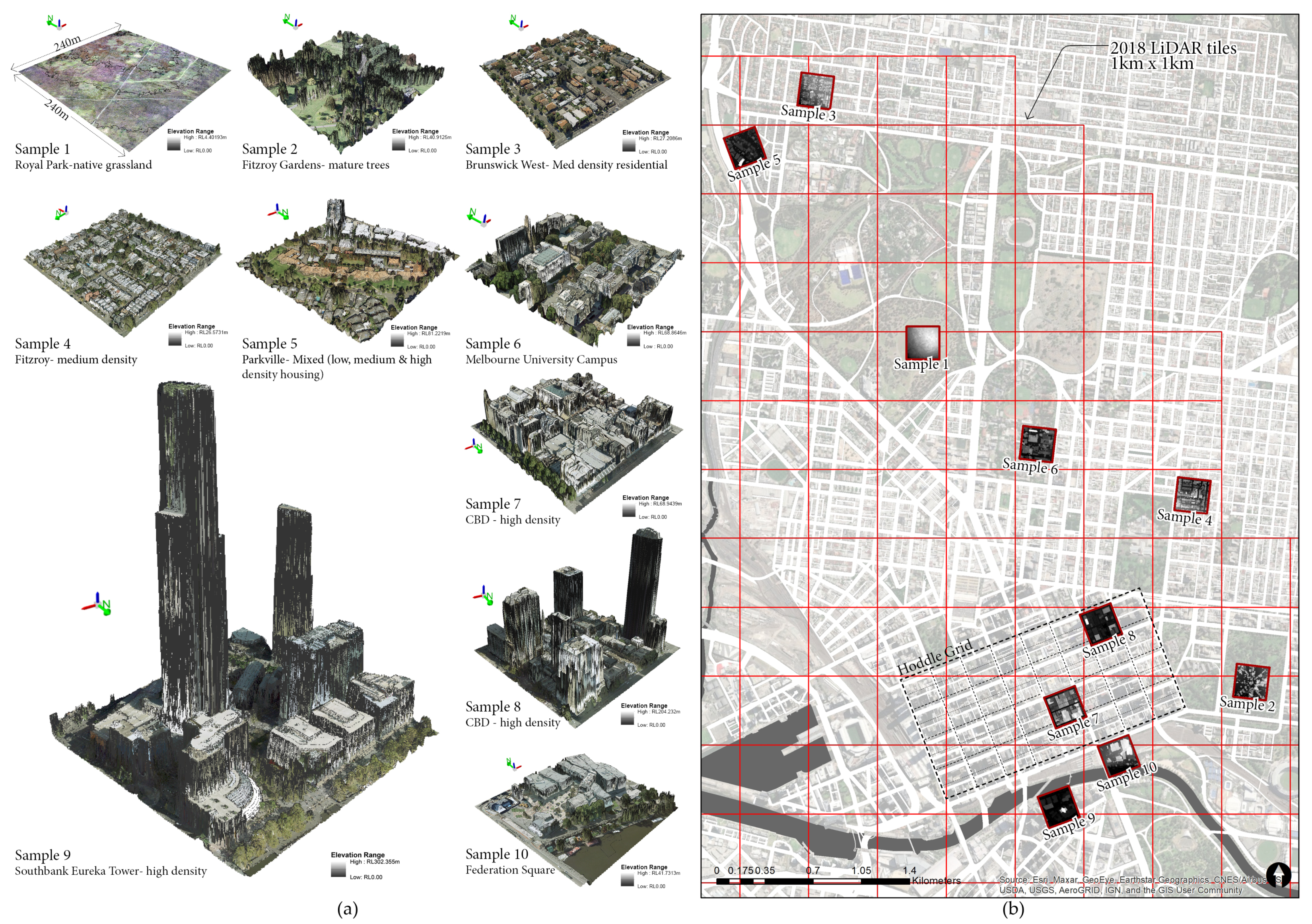
2.1. LiDAR-Derived DSM Samples

LiDAR provides promising applications for the 3D characterization of the earth’s surface [66]. It has distinctive advantages for collecting high-density data containing both vertical and horizontal information for natural and man-made structures and to show their relationships [67]. LiDAR data are extensively available in Australian cities as open data, which are being captured and updated periodically. The Intergovernmental Committee on Surveying and Mapping (ICSM) is the representative of the Australian states, territories and New Zealand and provides unlimited LiDAR data through its platform (ELVIS).
In addition to this, the City of Melbourne provided the 3D point cloud captured in 2018 through its Open Data platform [68]. The 3D point cloud representing all physical features (buildings, trees and terrain) has been encoded into a LAS format containing geospatial coordinates and RGB values for each point for the area of the municipality. The das has been captured in Map Grid of Australia (MGA) Zone 55 projection and saved in the XYZ coordinated in 1 km × 1 km. LAS file format. The capture pixel size in 7.5 cm ground sample distance with 25 cm absolute accuracy. Potentially, LiDAR datasets can be combined with other active or passive sensing techniques to increase the resolution of a point cloud or for other purposes (tree species or canopy capture). However, the sourced LiDAR data were unclassified, which did not allow to separate the vegetation from the built elements or the ground to study separately, while this possibility exists through sourcing classified LAS data.
These data have been used in this research to model a DSM from the point cloud and to study the complexity of urban fabric through fractal dimension. A DSM was created in GIS (ArcMap 10.6) with a raster resolution of 0.5 m by 0.5 m including landform, built and natural elements. The extent of data covers approximately a 1–5 km radius area around the Melbourne central business district (CBD), which includes the centre and inner-city suburbs. This area is characterized by the high-density area near the Yarra River surrounded by public gardens, parks, open spaces and infrastructure corridors. The urban density decreases as the distance increases from CBD and displays a wide range of variations of the urban fabric, from commercial districts to residential subdivisions. This variation provided a suitable context to identify multiple samples for fractal analysis.
The Melbourne CBD is formed by a grid named Hoddle Grid, which was established in 1837. The grid covers an area of 1 × 0.5 mile, using blocks of 10 × 10 chains (approximately 200 m). Hence, a sample of size of 240 m × 240 m was adopted to capture a block of land defined by the road structure. This block size was considered an optimal size to capture different characteristics of the urban fabric across the defined geographic area. Moreover, this sample size was considered a suitable size for the voxelization process to optimize the computation process. The module boundary was rotated to align the urban character, including building arrangements and streetscapes across central Melbourne.
Ten samples across the study area were extracted from the DSM for analysis (Figure 1a). The original elevation data were captured in the Australian Height Datum (AHD), which is relative to an approximate mean sea level (MSL). For this paper, all DSM samples were shifted to zero as a Reduced Level (RL) to create consistency for fractal analysis. These samples vary in terms of characteristics defined by the pattern of built form heights, streetscapes, vegetation, landform, slope and elevation. Moreover, two city landmarks were selected as part of the variations. The characteristics of selected samples are summarized in Table 1. Figure 1b displays the location of samples and their 3D configurations by overlaid aerial imagery on DSM samples.

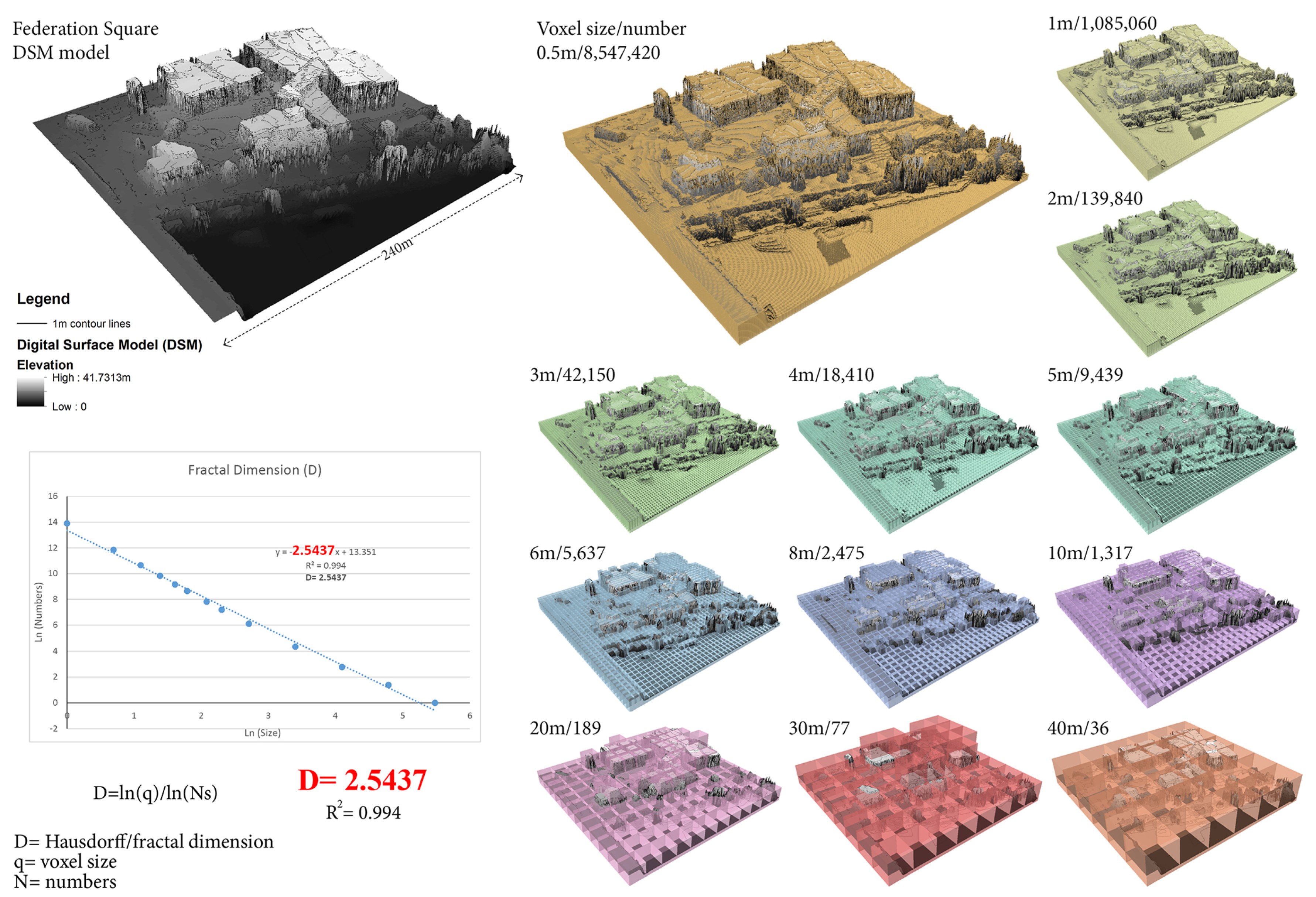
2.2. Estimating D Using Voxels

The voxelization method was previously applied to estimate the complexity of the visual bowl in Melbourne CBD [69]. It was developed in Rhinoceros and Grasshopper as a 3D computer-aided design platform supported by a visual programming language environment. In this paper, the voxelization method is implemented in GIS through resampling functionality and conversions from raster to vector data. The automation of this workflow in ArcGIS 10.6 using Model Builder allowed estimation of D for multiple selected samples.
In this research, the box-counting method was applied to three-dimensional patterns by applying voxel sizes of s(x) × s(y) × s (z) as cubes or voxels to estimate D values of a DSM of urban environments. DSM is a raster data, including cells at certain resolutions that store the elevation of features on the ground, which results in a complex surface. Raster cells replicate the voxels so that their sizes can be changed in the box-counting method to estimate the number of cells that cover the whole raster. In addition to two axes of boxes (x & y), the DSM include z values that need to be covered by voxels to calculate the overall number of voxels required to cover the raster at different resolutions.
The voxelization technique was implemented in GIS (ArcGIS 10.6) through raster operations and transformations of raster data to vector data to visualise voxels in 3D to see how they cover the DSM at different sizes. Determining the most appropriate voxel/grid sizes was considered to be one of the challenges for estimating D. The size of the grids used for the voxelization can be an even or an odd number; the range of grid size can be a succession of integers [5]. In this study, after a series of tests and calibrations, we employed a 240 m by 240 m DSM model at 0.5 m × 0.5 m cell size and estimated the number of the voxel at 0.5 m, 1, 2, 3, 4, 5, 6, 8, 10, 20, 30, 40, 60, 120 and 240 m voxels to estimate D for all samples. Figure 2 displays the voxelization results in 3D at different sizes for Federation Square on the edge of Melbourne CBD (Sample 10). The DSM model includes the built form and surrounding trees adjacent to the Yarra River.

2.3. Raster Analysis and Correlation to D

In addition, other related surface analytical methods were applied on selected samples to compute additional morphological attributes and correlate them with the estimated fractal dimensions. Indeed, in order to evaluate the potential of the method and its relevance for urban morphology studies, several urban form parameters were compared for their correlation with the estimated values of D.

2.3.1. Raster Elevation and Volume

Elevation is the key attribute of LiDAR point clouds and DSMs. The variations of elevation across a DSM reflects the height information of all features including ground, vegetation and buildings as a grid of squares. Moreover, the form of DSM is the reflection of feature volumes under the surface. Although tree canopies are not solid and can be seen through, in the DSM they appear as solid forms without gaps under the canopy. The elevation changes reflect different variations of an urban character represented by building heights and vegetation. Hence, elevation variables, such as maximum, minimum, mean and standard deviations, were calculated for each sample using raster statistics in GIS. The volume under the DSM was calculated using the raster volume function.

2.3.2. Solar Radiation

In this study, we compared solar radiation of DSM samples in relation to the estimated D by the voxelization method. The Area Solar Radiation tool available in ArcGIS 10.6 was used to calculate the insolation across the entire urban landscape. Solar radiation is conducted for multiple days during the summer season in Melbourne (December to February) with 10 days intervals and 30 min intervals. The output radiation rasters are a floating-point type with units of watt-hour per square meter (WH/m2). The latitude for the site area is used in calculations of solar declination and solar position. The calculations are repeated for each sample as the input topographic surface producing insolation maps for DSM samples. The minimum, maximum, mean and standard deviations were recorded for each sample for the correlation analysis.

2.3.3. Roughness

In this study, roughness is quantified by the deviation of the normal vector from its ideal form. In GIS, surface roughness is calculated by the largest inter-cell difference of a central pixel and its neighbouring cells. The calculation of the roughness plays a role in the analysis of elevation data. The algorithm is derived from the GDAL DEM utility available in QGIS 3.2. The maximum mean value and standard deviation were calculated for each sample. The roughness raster visually highlights the edges of DSM of a model including all elements. As the height changes become more dramatic, the defined edges become more evident in the resulted raster.
Therefore, the chosen parameters to be compared to D were:
  • the maximum and average elevation in each sample, as well as the standard deviation.
  • the volume of the digital elevation model (DEM) of each sample;
  • the minimum, maximum and average solar radiation observed on each sample as well as the standard deviation.
  • their maximum and average roughness as well as the standard deviation.
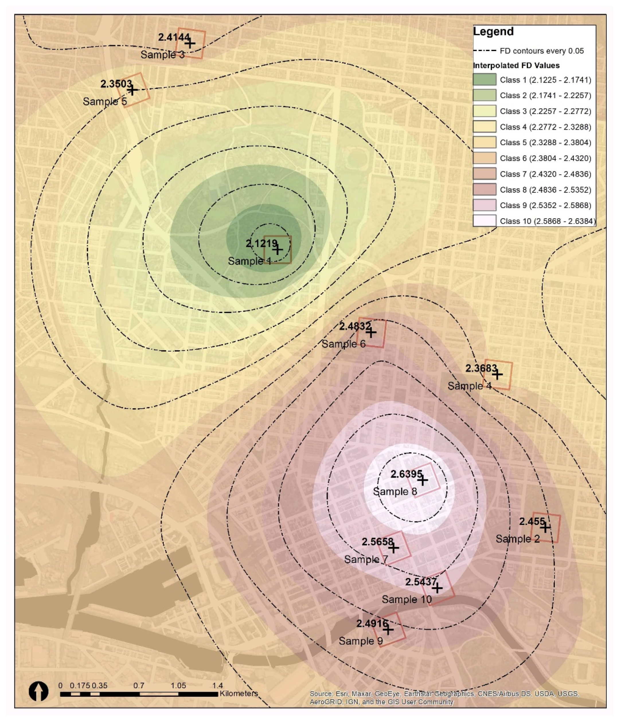
Statistically significant correlations were estimated using a non-parametric correlation test Spearman’s rho on SPSS. Additionally, Kriging interpolation was applied to understand the distribution of D values across central Melbourne.

3. Results

3.1. Fractal Dimension

The fractal dimension (D) was estimated for all ten DSM samples (Figure 1a) using the voxelization method in GIS (Table 2) with a consistent size of samples (240 m by 240 m). The voxelization method resulted in a set of D values that could be used to compare other sample attributes. Estimated D values for all samples ranged between 2.1219 (lowest) and 2.6396 (highest). The inclusion of a nearly flat surface (sample 1) allowed us to have a control sample to relate the effect of built and natural elements to changing D values. The calculated coefficient of determination (R2) was estimated between 0.9891 to 0.9956, which indicates that strong linear scaling relationships occur across all DSM samples due to their having a high fractal quality.
A visual comparison of DSM samples based on their D values indicated the potential for D to be a descriptor of urban character. Visually, D values increased with the intensification of features (built and vegetation) across all samples, as well as with landform changes. Higher D values were estimated for dense areas (samples 7, 8 and 9) compared to medium density samples (samples 3 and 4). Very close-range D values were estimated for similar character samples (samples 3 and 4 or samples 6 and 7). Minor differences in urban character, such as with built form style, tree canopy size or street layout, resulted in slightly different D values. Sample 10 showed the effect of landform change (from the river to street level) that increased the D value.
The estimated D values revealed the effectiveness of the proposed method for numeric characterisation of urban areas. D values reflect the distinct, recognisable pattern of elements and attributes that make one sample different from the other. The numerical characterisation of selected samples supports the serial vision experience of the urban context presented in Figure 3 using Kriging interpolation of FD values. Although it is a coarse representation of D values across central Melbourne, based on only 10 samples, it reflects the variations of character from low to high urban density in association with open spaces, which correlates with the physical form of the city. Therefore, the CBD results in the highest D values.

3.2. DSM Analysis and Measurements

The variations of DSM elevations were plotted in a hypsometric curve (Figure 4a). The curve reflects the differences in elevation across each DSM sample due to their different characteristics, including natural and built elements. The graph highlights sample 8 as the highest D and potential volume created by the DSM. The area under the curve highlighted the volume under the curve that can be another relative variable to D values. Hence, maximum, mean, standard deviation and volume were calculated for all samples for comparison with D (Table 2).
Solar radiation area was calculated in ArcGIS 10.6. The sample alignments to the north direction are slightly inconsistent across all samples, which can reduce the confidence of the judgement. The solar radiation was simulated for all samples in GIS during the summer months.
The surface roughness analysis conducted in QGIS 3.2.3 provided another layer of raster analysis in this study (Figure 4b). The result of the analysis provided an interesting visual output to reflect the effect of DSM components, including built and natural elements resulting in surface irregularities. As the normal deviation increases with vertical building surfaces, the roughness measure increases. The maximum surface roughness was estimated for samples 8 and 9, which had the tallest built forms compared to other samples. Maximum, mean and standard deviation were recorded for surface roughness for correlation analysis with D.

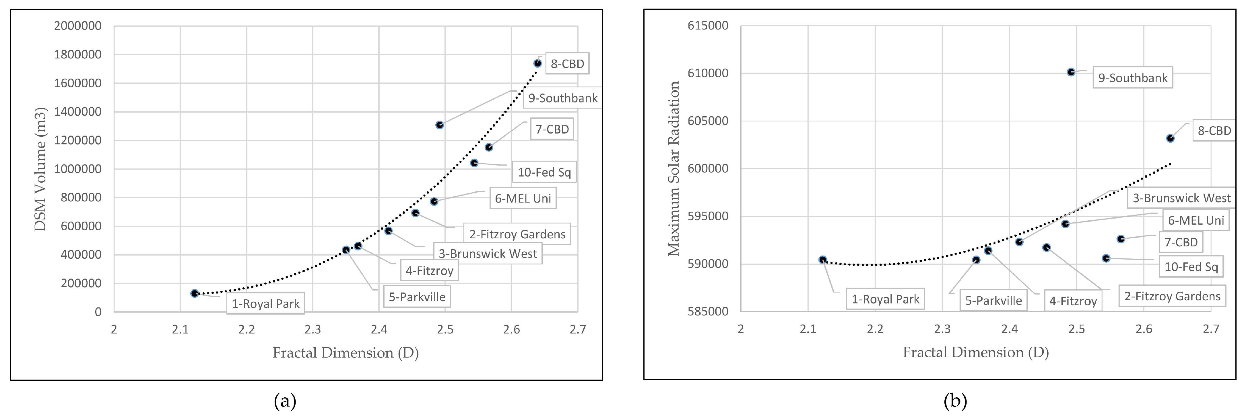
3.3. Correlation of D to Other Urban Form Parameters

The analysis of correlations between D and other urban form parameters across the samples revealed a strong association between variables. Overall, D was found to be significantly correlated to each parameter, to various degrees (Table 3).
Specifically, the correlation between D and the elevation parameters indicated that, while there was no relationship between D and maximum building height, D has a strong correlation between mean height across samples and the DSM volume (Figure 5a). The importance of mean height and volume highlights the positive effect of consolidation and compactness of an urban context in driving D values and overall visual complexity.
Although the values of the estimated solar radiation were found to be correlated to other estimated parameters, such as elevation and roughness, only the maximum solar radiation was found to be significantly correlated with D (Figure 5b). The estimated D values based on the voxelization method did not show any correlation with modelled roughness surfaces, except for the standard deviation of values within the sample.
Surface roughness appeared to be an independent variable compared to the estimated fractal dimension. Hence, roughness, as another descriptor of structural complexity, was correlated with the raster measurements. This indicates that roughness mean values presented positive correlations with elevation (std. d.) and raster volume and strong negative relationships with the mean solar radiation (Table 4).

4. Discussion and Conclusions

The application of the ‘box-counting’ method in 3D using voxels on DSMs provides new possibilities to analyse urban landscapes. It allowed studying the complexity of urban fabric in a 3-dimensional fashion to study urban character. The analysis applied at a broader geographical area to include a larger coverage of distinct, recognisable and consistent patterns of elements and attributes for numerical comparison. This has as yet received little attention in the literature where urban character has not been systematically and empirically studied before in an urban context using high-quality remote sensing data. Estimated D values provided a numerical characterization for comparison of urban environments.
The results revealed that the fractal dimension calculated using the voxelization method is significantly influenced by the physical volume of the space. Increasing building heights across the sample area has a positive effect on increasing complexity as reported similarly in previous research [69]. The voxelization technique developed in GIS provided higher control and accuracy over the voxelization process compared to the previous workflow presented by Tara et al. [69] This provides opportunities to implement it on larger scale elevation models by leveraging the possibilities in GIS using open data, DEM, DSM and satellite imagery. DSM models and voxelization provide new methods of interpretation and understanding previously subjective concepts of built environments. The capabilities of classified LiDAR data to separate urban features provides other opportunities for analysis of urban form through its separate built and natural elements.
Furthermore, the fractal analysis in this study was conducted on ten urban character samples to understand the variations of complexity across different parts of Melbourne Central. This was a very different approach to previous research [69]. In this paper, attention was given specifically to samples of different urban forms, which differed from analysing the user experience through a visibility factor, which previously simulated viewshed or visual bowl interpretation in 3D.
The proposed research provides a new approach to studying the fractal dimension in urban environments compared to the previous research [2,10,11,12,47,70]. Using a LiDAR-derived DSM for fractal analysis by using a 3D box-counting method, this work provides a novel approach to studying urban and non-urban environments. Studying complexity by a volumetric approach appears to be a suitable approach to study urban environments due to the volumetric nature of urban contexts with considerable variation in built form and vegetation. The level of voxelization can be adjusted to suit raster models on any scale to estimate fractal dimensions.

4.1. Limitations of the Method

This paper intends to present a new method of fractal analysis and its potential for future research. The results presented here should be understood as preliminary. In this context, the values of other urban form parameters, which were chosen for the raster analysis, should also be regarded critically. In particular, in the case of the estimation of solar radiation area, the sample alignments to the north are slightly inconsistent across all samples, which could reduce confidence in the measurement of solar radiation area.
Furthermore, multiple limitations were identified during the course of this research which could be considered opportunities for future testing and experimentation. Firstly, the sourced open LiDAR was unclassified, which did not allow the separation of landform, buildings and vegetation for the study of the effect of each entity on D values separately. Potentially a classified LiDAR file can be sourced from municipalities to test this scenario. Secondly, the developed voxelization workflow was semi-automated, which made it a slightly time-consuming process to estimate each D value. Potential future automation of this process would allow us to test it on higher numbers of samples across the city and increase the resolution of fractal dimensions estimated in different scales (Figure 3).
In general, the DSM provides a simplistic representation of the urban fabric, which omits a considerable amount of detail, including architectural and vegetation details. Moreover, it does not differentiate between hard and soft surfaces. It is unable to present gaps under bridges or tree canopies due to vertical projection of planar heights or elevations. However, it was capable of representing a simplified structural form of an urban context for the purpose of this study.

4.2. Potential for Applications

The proposed research has potential applications in the current context of Australian cities. With a fast-growing population and climate change impacts, Australian cities are aiming to transform from low-density suburban to more compact and become more sustainable, liveable, resilient and inclusive places to live. Greater urban density is considered to be more effective in providing lower per capita infrastructure costs, a wider variety of housing types and greater affordability [71]. However, achieving this will be a constant challenge for state and local governments, the property development industry and the community. Infill development, urban consolidation and intensification are some of the strategies being used in these cities to increase density around defined centres or along corridors, which results in a significant change to the urban form. Moreover, the concept of the 20-min neighbourhood [72] in established suburbs or greenfield developments could be investigated using the proposed method to speculate on optimum urban forms in relation to liveability, physical and mental health factors. This research proposes that the higher the D value, the more structurally complex is an urban environment. Complexity linked to ambiguity in urban environments has the potential to inform future environmental design and planning [40].
Likewise, this research could be extended to study the evolution and change of urban fabric similar to Qin et al. [17] or for comparing the urban form of different cities. The collective differences of social, cultural and political processes in shaping cities can be studied using fractal analysis, voxelization and DSMs. The proposed method can be used in impact assessments to study the impact of new developments in an existing urban context.
Furthermore, the proposed method has implications for studying peri-urban, rural and regional landscapes. Considering the novel aspects of this research, it can be considered as a continuation and evolution of previous research in estimating D values in 3D [17,73,74]. Similarly, the voxelization method could be used with different landforms in rural areas to understand variations of landform and complexity, which are likely to evoke different human preferences and experiences. Finally, this fractal research could be extended to climate change research by considering the complexity of the physical landscape, whether natural or built, in relation to performance factors, environmental or biodiversity indicators.

Author Contributions

Conceptualization, A.T. and A.P.; Data curation, A.T.; Formal analysis, A.T. and A.P.; Investigation, A.T. and A.P.; Methodology, A.T.; Software, A.T.; Supervision, G.L.; Visualization, A.T.; Writing—original draft, A.T. and A.P.; Writing—review and editing, G.L. All authors have read and agreed to the published version of the manuscript.

Funding

The research had no funding.

Institutional Review Board Statement

Not applicable.

Informed Consent Statement

Not applicable.

Data Availability Statement

The data presented in this study are available on request to the corresponding author.

Acknowledgments

The authors would like to thank the City of Melbourne for providing LiDAR data 2018 as an open-source that allowed conducting the research.

Conflicts of Interest

The authors declare no conflict of interest.

References

  1. Batty, M.; Longley, M. Fractal Cities—A Geometry of Form and Function; Academic Press: London, UK, 1994. [Google Scholar]
  2. Vaughan, J.; Ostwald, M.J. Using fractal analysis to compare the characteristic complexity of nature and architecture: Re-examining the evidence. Archit. Sci. Rev. 2010, 53, 323–332. [Google Scholar] [CrossRef]
  3. Perry, S. The Unfinished Landscape—Fractal Geometry and the Aesthetic of Ecological Design. Ph.D. Thesis, Queensland University of Technology, Brisbane City, Austrilia, 2012. [Google Scholar]
  4. Mandelbrot, B.B. The Fractal Geometry of Nature, Henry Holt and Company; Cambridge University Press: Cambrige, UK, 1982. [Google Scholar]
  5. Taud, H.; Parrot, J.-F. Measurement of DEM roughness using the local fractal dimension. Géomorphol. Relief Process. Environ. 2006, 11, 327–338. [Google Scholar] [CrossRef] [Green Version]
  6. Thomas, I.; Frankhauser, P.; De Keersmaecker, M.-L. Fractal dimension versus density of built-up surfaces in the periphery of Brussels. Pap. Reg. Sci. 2007, 86, 287–308. [Google Scholar] [CrossRef]
  7. Cartwright, T.J. Planning and Chaos Theory. J. Am. Plan. Assoc. 1991, 57, 44–56. [Google Scholar] [CrossRef]
  8. Batty, M. Cities and Complexity: Understanding Cities with Cellular Automata, Agent-Based Models, and Fractals; MIT Press: Cambridge, MA, USA, 2005. [Google Scholar]
  9. Cardillo, A.; Scellato, S.; Latora, V.; Porta, S. Structural properties of planar graphs of urban street patterns. Phys. Rev. E 2006, 73, 066107. [Google Scholar] [CrossRef] [Green Version]
  10. Cooper, J.; Oskrochi, R. Fractal Analysis of Street Vistas: A Potential Tool for Assessing Levels of Visual Variety in Everyday Street Scenes. Environ. Plan. B Plan. Des. 2008, 35, 349–363. [Google Scholar] [CrossRef] [Green Version]
  11. Stamps, A.E. Fractals, skylines, nature and beauty. Landsc. Urban Plan. 2002, 60, 163–184. [Google Scholar] [CrossRef]
  12. Chalup, S.K.; Henderson, N.; Ostwald, M.J.; Wiklendt, L. A Computational Approach to Fractal Analysis of a Cityscape’s Skyline. Archit. Sci. Rev. 2009, 52, 126–134. [Google Scholar] [CrossRef]
  13. Chalup, S.K.; Ostwald, M.J. Anthropocentric Biocybernetic Approaches to Architectural Analysis: New Methods for Investigating the Built Environment. In Built Environment: Design Management and Applications; The University of Newcastle: Callaghan, Australia, 2010. [Google Scholar]
  14. Tucker, C. Developing Computational Image Segmentation Techniques for the Analysis of the Visual Properties of Dwelling Facades within a Streetscape. Ph.D. Thesis, University of Newcastle, Callaghan, Australia, 2004. [Google Scholar]
  15. Cooper, J. Fractal Assessment of Street-level Skylines: A Possible Means of Assessing and Comparing Character. Urban Morphol. 2003, 7, 73–82. [Google Scholar]
  16. Cooper, J. Assessing Urban Character: The use of fractal analysis of street edges. Urban Morphol. 2005, 9, 95–107. [Google Scholar]
  17. Qin, J.; Fang, C.; Wang, Y.; Li, Q.; Zhang, Y.A. three dimensional box-counting method for estimating fractal dimension of urban form. Geogr. Res. 2015, 34, 85–96. [Google Scholar]
  18. Chen, Y. Fractal Modeling and Fractal Dimension Description of Urban Morphology. Entropy 2020, 22, 961. [Google Scholar] [CrossRef] [PubMed]
  19. Bovill, C. Fractal Geometry in Architecture and Design, Birkhäuser; Birkhäuser: Boston, MA, USA, 1996. [Google Scholar]
  20. Sala, N. Fractals in Architecture: Some Examples. In Fractals in Biology and Medicine; Losa, G.A., Merlini, D., Nonnenmacher, T.F., Weibel, E.R., Eds.; Birkhäuser: Basel, Switzerland, 2002. [Google Scholar]
  21. Ostwald, M.J.; Tucker, C. Calculating Characteristic Visual Complexity in the Built Environment: An Analysis of Bovill’s Method; CIB WO92 Procurement: Hunter Valley, NSW, Australia, 2007. [Google Scholar]
  22. Ostwald, M.J.; Vaughan, J.; Tucker, C. Characteristic Visual Complexity: Fractal Dimensions in the Architecture of Frank Lloyd Wright and Le Corbusier; Birkhäuser: Cham, Switzerland, 2008. [Google Scholar]
  23. Ostwald, M.J.; Vaughan, J. The Fractal Dimension of Architecture; Springer International Publishing: Newcastle, Australia, 2016. [Google Scholar]
  24. Jiménez, J.; López, A.M.; Cruz, J.; Esteban, F.J.; Navas, J.; Villoslada, P.; Ruiz De Miras, J. A Web platform for the interactive visualization and analysis of the 3D fractal dimension of MRI data. J. Biomed. Inform. 2014, 51, 176–190. [Google Scholar] [CrossRef] [Green Version]
  25. Gao, P.; Cushman, S.A.; Liu, G.; Ye, S.; Shen, S.; Cheng, C. FracL: A Tool for Characterizing the Fractality of Landscape Gradients from a New Perspective. ISPRS Int. J. Geo-Inf. 2019, 8, 466. [Google Scholar] [CrossRef] [Green Version]
  26. Ai, T.; Ru, Z.; Zhou, H.; Pei, J.L. Box-counting methods to directly estimate the fractal dimension of a rock surface. Appl. Surf. Sci. 2014, 314, 610–621. [Google Scholar] [CrossRef]
  27. Liu, Y.; Chen, L.; Wang, H.; Jiang, L.; Zhang, Y.; Zhao, J.; Wang, D.; Zhao, Y.; Song, Y. An improved differential box-counting method to estimate fractal dimensions of gray-level images. J. Vis. Commun. Image Represent. 2014, 25, 1102–1111. [Google Scholar] [CrossRef]
  28. Wang, Q.; Liang, Z.; Wang, X.; Zhao, W.; Wu, Y.; Zhou, T. Fractal analysis of surface topography in ground monocrystal sapphire. Appl. Surf. Sci. 2015, 327, 182–189. [Google Scholar] [CrossRef]
  29. Oxford English Dictionary, 2nd ed.; Oxford University Press: Oxford, UK, 2004.
  30. Graham, N.A.J.; Nash, K.L. The importance of structural complexity in coral reef ecosystems. Coral Reefs 2012, 32, 315–326. [Google Scholar] [CrossRef]
  31. Yanovski, R.; Nelson, P.A.; Abelson, A. Structural Complexity in Coral Reefs: Examination of a Novel Evaluation Tool on Different Spatial Scales. Front. Ecol. Evol. 2017, 5, 27. [Google Scholar] [CrossRef] [Green Version]
  32. Bai, X.; Nath, I.; Capon, A.; Hasan, N.; Jaron, D. Health and wellbeing in the changing urban environment: Complex challenges, scientific responses, and the way forward. Curr. Opin. Environ. Sustain. 2012, 4, 465–472. [Google Scholar] [CrossRef] [Green Version]
  33. Ives, C.D.; Kelly, A.H. The coexistence of amenity and biodiversity in urban landscapes. Landsc. Res. 2016, 41, 495–509. [Google Scholar] [CrossRef]
  34. Sepe, M.; Pitt, M. The characters of place in urban design. Urban Des. Int. 2014, 19, 215–227. [Google Scholar] [CrossRef]
  35. Ode, Å.; Tveit, M.S.; Fry, G. Capturing Landscape Visual Character Using Indicators: Touching Base with Landscape Aesthetic Theory. Landsc. Res. 2008, 33, 89–117. [Google Scholar] [CrossRef]
  36. Ewing, R.; Handy, S. Measuring the Unmeasurable: Urban Design Qualities Related to Walkability. J. Urban Des. 2009, 14, 65–84. [Google Scholar] [CrossRef]
  37. Laverick, C. Visual complexity in the urban landscape. Landsc. Res. 1980, 5, 14–15. [Google Scholar] [CrossRef]
  38. Lynch, K. The Image of the City, Cambridge, Mass; The MIT Press: Cambridge, MA, USA, 1960. [Google Scholar]
  39. Cullen, G. The Concise Townscape; Architectural Press: Hudson, NY, USA, 1971. [Google Scholar]
  40. Rapoport, A.; Kantor, R.E. Complexity and Ambiguity in Environmental Design. J. Am. Inst. Plan. 1967, 33, 210–221. [Google Scholar] [CrossRef]
  41. Rapoport, A.; Hawkes, R. The Perception of Urban Complexity. J. Am. Inst. Plan. 1970, 36, 106–111. [Google Scholar] [CrossRef]
  42. Repton, H. Observations on the Theory and Practice of Landscape Gardening: Including Some Remarks on Grecian and Gothic Architecture, Collected from Various Manuscripts, in the Possession of the Different Noblemen and Gentlemen, for Whose Use They Were Originally Written; the Whole Tending to Establish Fixed Principles in the Respective Arts; T. Bensley: London, UK, 1803. [Google Scholar]
  43. Eisenman, R.; Rappaport, J. Complexity preference and semantic differential ratings of complexity-simplicity and symmetry-asymmetry. Psychon. Sci. 1967, 7, 147–148. [Google Scholar] [CrossRef]
  44. Vitz, P.C.; Todd, T.C. A coded element model of the perceptual processing of sequential stimuli. Psychol. Rev. 1969, 76, 433–449. [Google Scholar] [CrossRef]
  45. Nasar, J.L. Environmental Aesthetics: Theory, Research, and Application; Cambridge University Press: Cambridge, UK, 1992. [Google Scholar]
  46. Nasar, J.L. The Evaluative Image of the City; Sage Publications: Thousand Oaks, CA, USA, 1998. [Google Scholar]
  47. Stamps, A.E., III. Entropy, visual diversity, and preference. J. Gen. Psychol. 2002, 129, 300–320. [Google Scholar] [CrossRef]
  48. Wei, D.; Hu, X.; Chen, Y.; Li, B.; Chen, H. An Investigation of the Quantitative Correlation between Urban Spatial Morphology Indicators and Block Wind Environment. Atmosphere 2021, 12, 234. [Google Scholar] [CrossRef]
  49. Adolphe, L. A Simplified Model of Urban Morphology: Application to an Analysis of the Environmental Performance of Cities. Environ. Plan. B Plan. Des. 2001, 28, 183–200. [Google Scholar] [CrossRef]
  50. Rind, D. Complexity and Climate. Science 1999, 284, 105–107. [Google Scholar] [CrossRef] [PubMed] [Green Version]
  51. Sarralde, J.J.; Quinn, D.J.; Wiesmann, D.; Steemers, K. Solar energy and urban morphology: Scenarios for increasing the renewable energy potential of neighbourhoods in London. Renew. Energy 2015, 73, 10–17. [Google Scholar] [CrossRef] [Green Version]
  52. Bernabé, A.; Musy, M.; Andrieu, H.; Calmet, I. Radiative properties of the urban fabric derived from surface form analysis: A simplified solar balance model. Sol. Energy 2015, 122, 156–168. [Google Scholar] [CrossRef]
  53. Morganti, M.; Salvati, A.; Coch, H.; Cecere, C. Urban morphology indicators for solar energy analysis. Energy Procedia 2017, 134, 807–814. [Google Scholar] [CrossRef]
  54. Robinson, D. Urban morphology and indicators of radiation availability. Sol. Energy 2006, 80, 1643–1648. [Google Scholar] [CrossRef]
  55. Mohajeri, N.; Gudmundsson, A.; Upadhyay, G.; Assouline, D.; Scartezzini, J.-L. Neighbourhood morphology and solar irradiance in relation to urban climate. In Proceedings of the 9th International Conference on Urban Climate jointly with 12th Symposium on the Urban Environment, Toulouse, France, 20–24 July 2015. [Google Scholar]
  56. Zhu, D.; Song, D.; Shi, J.; Fang, J.; Zhou, Y. The Effect of Morphology on Solar Potential of High-Density Residential Area: A Case Study of Shanghai. Energies 2020, 13, 2215. [Google Scholar] [CrossRef]
  57. Liang, J.; Gong, J. A Sparse Voxel Octree-Based Framework for Computing Solar Radiation Using 3D City Models. ISPRS Int. J. Geo-Inf. 2017, 6, 106. [Google Scholar] [CrossRef] [Green Version]
  58. Ng, E.; Yuan, C.; Chen, L.; Ren, C.; Fung, J.C.H. Improving the wind environment in high-density cities by understanding urban morphology and surface roughness: A study in Hong Kong. Landsc. Urban Plan. 2011, 101, 59–74. [Google Scholar] [CrossRef]
  59. Fuad, M. Coral Reef Rugosity and Coral Biodiversity; ITC Faculty Geo-Information Science and Earth Observation: North Sulawesi, Indonesia, 2010. [Google Scholar]
  60. Sun, W.; Xu, G.; Gong, P.; Liang, S. Fractal analysis of remotely sensed images: A review of methods and applications. Int. J. Remote. Sens. 2006, 27, 4963–4990. [Google Scholar] [CrossRef]
  61. Patuano, A.; Tara, A. Fractal Geometry for Landscape Architecture: Review of Methodologies and Interpretations. Landsc. Archit. 2020, 2020, 72–80. [Google Scholar]
  62. Bonczak, B.; Kontokosta, C.E. Large-scale parameterization of 3D building morphology in complex urban landscapes using aerial LiDAR and city administrative data. Comput. Environ. Urban Syst. 2019, 73, 126–142. [Google Scholar] [CrossRef]
  63. Dong, P.; Chen, Q. LiDAR Remote Sensing and Applications; Taylor Francis Group: Boca Raton, FL, USA, 2017. [Google Scholar]
  64. Panagiotakis, E.; Chrysoulakis, N.; Charalampopoulou, V.; Poursanidis, D. Validation of Pleiades Tri-Stereo DSM in Urban Areas. ISPRS Int. J. Geo-Inf. 2018, 7, 118. [Google Scholar] [CrossRef] [Green Version]
  65. Kaldor Public Art Projects 2021. Christo and Jeanne-Claude. Available online: https://kaldorartprojects.org.au/projects/project-1-christo-jeanne-claude/ (accessed on 8 June 2021).
  66. Kulawardhana, R.W.; Popescu, S.C.; Feagin, R.A. Airborne lidar remote sensing applications in non-forested short stature environments: A review. Ann. For. Res. 2017, 60, 173–196. [Google Scholar] [CrossRef] [Green Version]
  67. Wang, M.Z.; Merrick, J.R. Urban forest corridors in Australia: Policy, management and technology. Nat. Resour. Forum 2013, 37, 189–199. [Google Scholar] [CrossRef]
  68. City of Melbourne. 3D Point Cloud 2018. 2018. Available online: https://data.melbourne.vic.gov.au/City-Council/City-of-Melbourne-3D-Point-Cloud-2018/2dqj-9ydd (accessed on 8 November 2021).
  69. Tara, A.; Belesky, P.; Ninsalam, Y. Towards Managing Visual Impacts on Public Spaces: A Quantitative Approach to Studying Visual Complexity and Enclosure Using Visual Bowl and Fractal Dimension. J. Digit. Landsc. Archit. 2019, 4, 12. [Google Scholar]
  70. Hagerhall, C.M.; Purcell, T.; Taylor, R. Fractal dimension of landscape silhouette outlines as a predictor of landscape preference. J. Environ. Psychol. 2004, 24, 247–255. [Google Scholar] [CrossRef]
  71. Searle, G. Densifying the City? Government Policies and Accelerating Densification in Sydney; Edward Elgar Publishing: Cheltenham, UK, 2020. [Google Scholar]
  72. Victoria Government. Plan Melbourne (2017–2050). 2017. Available online: https://www.planning.vic.gov.au/policy-and-strategy/planning-for-melbourne/plan-melbourne (accessed on 2 February 2021).
  73. Goodchild, M.F.; Mark, D.M. The Fractal Nature of Geographic Phenomena. Ann. Assoc. Am. Geogr. 1987, 77, 265–278. [Google Scholar] [CrossRef]
  74. Goodchild, M.F. Fractals and the accuracy of geographical measures. J. Int. Assoc. Math. Geol. 1980, 12, 85–98. [Google Scholar] [CrossRef]
Figure 1. (a) Selected 10 DSM samples (240 m × 240 m) in a perspective view, showing the composition of landform, vegetation and built forms; (b) Location of selected samples in Melbourne covered by LiDAR tiles 2018.
Fractalfract 05 00227 g001
Figure 2. Sample voxelization of DSM (Federation Square) in GIS and estimation of Fractal Dimension (D).
Fractalfract 05 00227 g002
Figure 3. Kriging interpolation of D values of 10 samples across central Melbourne.
Fractalfract 05 00227 g003
Figure 4. (a) Plot of the hypsometric curve showing the proportions of sample area that exist at various elevations. (b) Raster analysis in GIS including solar radiation and surface roughness for ten studied samples.
Fractalfract 05 00227 g004
Figure 5. (a) Correlation of D and DSM Volume; (b) Correlation of D and Max. Solar Radiation (showing the measurements and polynomial regression line).
Fractalfract 05 00227 g005
Table 1. Summary of sample’s characteristics.
SampleCharacteristics [Elevation]
Sample 1Royal park native grassland, a very gentle slope without any features [RL0.0 to RL4.4 m]
Sample 2Centre of Fitzroy Gardens, mostly mature trees natural setting [RL0.0 to RL 40.9 m]
Sample 3Brunswick West-medium density residential [RL0.0 to RL27.2 m]
Sample 4Fitzroy-medium density residential [RL0.0 to RL26.57 m]
Sample 5Parkville- Mixed density, low to a high residential density [RL0.0 to RL81.20 m]
Sample 6Melbourne University Campus represents a medium to high-density context with mature trees [RL0.0 to RL68.86 m]
Sample 7CBD high-density area [RL0.0 to RL68.94 m]
Sample 8CBD high-density area [RL0.0 to RL204.23 m]
Sample 9Southbank high-density area including city landmark Eureka Tower [RL0.0 to RL302.23 m]
Sample 10Federation Square- a landmark in CBD [RL0.0 to RL41.73 m]
Table 2. DSM measurements (elevation max, mean, standard deviation and volume).
SampleEstimated DElevation Max. (m)Elevation Mean (m)Elevation (std. d.)Volume (m3)
Sample 12.12194.42.430.79129,369.23
Sample 22.45540.9112.48.39692,034.71
Sample 32.414427.210.183.76566,997.51
Sample 42.368326.58.394.47460,849.63
Sample 52.350381.27.766.77433,921.66
Sample 62.483268.8613.949.01772,763.14
Sample 72.565868.920.3114.381150,447.44
Sample 82.6395204.23231.0733.291,738,956.08
Sample 92.4916302.35523.3742.371,307,388.32
Sample 102.543741.7318.2810.891,041,751.73
Table 3. Correlation table (N = 10). Only significant correlations are included.
Spearman’s RhoFractal Dimension (D)
Correlation CoefficientSig. (2-Tailed)
Elevation Mean (m)0.9640.000
Elevation std. d. (m)0.8790.001
Volume (m3)0.9640.000
Solar Radiation Max. (WH/m2)0.6970.025
Roughness (std. d.)0.6850.029
Table 4. Correlation table (N = 10). Only significant correlations are included.
Spearman’s RhoRoughness (Mean)
Correlation CoefficientSig. (2-Tailed)
Elevation std. d. (m)0.721<0.05
Volume (m3)0.636<0.05
Solar Radiation Mean. (WH/m2)−0.988<0.005
Publisher’s Note: MDPI stays neutral with regard to jurisdictional claims in published maps and institutional affiliations.

