Fractal Methods and Power Spectral Density as Means to Explore EEG Patterns in Patients Undertaking Mental Tasks

Abstract

Brain electrical activity recorded as electroencephalogram data provides relevant information that can contribute to a better understanding of pathologies and human behaviour. This study explores extant electroencephalogram (EEG) signals in search of patterns that could differentiate subjects undertaking mental tasks and reveals insights on said data. We estimated the power spectral density of the signals and found that the subjects showed stronger gamma brain waves during activity while presenting alpha waves at rest. We also found that subjects who performed better in those tasks seemed to present less power density in high-frequency ranges, which could imply decreased brain activity during tasks. In a time-domain analysis, we used Hall–Wood and Robust–Genton estimators along with the Hurst exponent by means of a detrented fluctuation analysis and found that the first two fractal measures are capable of better differentiating signals between the rest and activity datasets. The statistical results indicated that the brain region corresponding to Fp channels might be more suitable for analysing EEG data from patients conducting arithmetic tasks. In summary, both frequency- and time-based methods employed in the study provided useful insights and should be preferably used together in EEG analysis.

1. Introduction

There is a myriad of physiological processes in biological systems [1] that enable an organism to perform multiple activities. The modelling of these phenomena is a challenging task wherein different mathematical techniques capable of adequately describing such models have been employed [2,3,4,5,6]. The brain is composed of a complex network of actions and reactions working in a coordinated effort to control several processes in the whole body. These networks incorporate a mixture of integration, differentiation, feedback loops, and other regulatory mechanisms that enable an organism to perform multiple activities, a quality typical of complex systems with time-adaptable features. Considering their non-stationary behaviour, modelling these phenomena is a very challenging task. Electrical activity can provide significant information about the dynamics pertaining to the behaviour of brain systems [7].

A record of the brain electrical activity can be obtained by means of an electroencephalogram (EEG). EEG signals are the essence of the synchronous electrical activity of neuronal cells, which change their membrane potentials according to mental, motor, and sensory activities. These signals contain relevant information that can contribute to a better understanding of brain activity and to the diagnosis and treatment of several different pathologies, especially those with psychiatric and neurophysiological origins. In this context, EEG signals comprise valuable information for better understanding brain activity since they are influenced by both physiological and exogenous factors and have random characteristics. Indeed, there is an increasing demand for novel medical therapies with lower costs and higher efficiencies, motivating several researchers from different fields of knowledge, including physicians, physicists, and engineers, towards the same goal.

EEG signals can be obtained through the use of invasive and noninvasive electrodes. Noninvasive electrodes are widely used for their convenience and allow for capturing information with less risk to the patient. Invasive electrodes are mainly used when one needs to capture information from an internal region of the brain where noninvasive electrodes are insufficient. In general, typical EEG equipment uses noninvasive electrodes normally placed in caps or attached to the scalp [8]. Usually, EEG data collection follows standards such as the International 10/20 scheme, which is detailed in Section 3.

EEG analyses can be employed in cases of epilepsy [9,10] or clinical suspicion of this disease [11]; in patients with altered consciousness; and for diagnostic evaluations of patients with other neurological (i.e., infectious [12], degenerative [13]), and psychiatric diseases [14]. Furthermore, EEG can also be employed to investigate behavioural aspects (disease-related or not). It has been used to assess sleep quality, to characterise sleep stages [15], and even to identify underlying disorders [16,17]. Recent fields of study concerning EEG conduct predictions and analyses of the performance pertaining to mobile cognition including sports competition [18], stress and emotional regulation [19], the identification of drowsiness/alertness patterns [20], and even the exploration of the effect of music on the brain [21].

Still concerning performance and cognition, EEG has also been used as a source for exploring and classifying signals during complex mental activities [22], including arithmetic tasks, which usually demand several simultaneous cognitive processes and strategies. Different approaches have been employed for EEG analysis on that note, mostly related to machine learning, such as neural networks based on particle swarm optimisation [23] and other approaches trying to avail real-time performance recognition [24]. In general, several studies have focused on identifying EEG patterns using different methods that can detect and quantify both linear and nonlinear mechanisms and, therefore, somehow reflect patients’ specific characteristics (pertaining to diseases or cognitive aspects) [25,26,27,28,29,30,31,32,33].

Recently, the implementation of computational intelligence towards the analysis of EEG signals in light of brain–computer interfaces has become an increasingly expanding and promising field concerning health and behavioural applications [34]. While this vast field broadens several different tools that have been used to classify and recognise EEG patterns, such as autoregressive models [35], mode decomposition [36], and pattern recognition [37], there seems to be a significant advantage of classifications employing a particular machine learning subfield: deep learning models [38].

Based on multilayer neural networks, deep learning models are a family of supervised-learning algorithms usually tailored very carefully for a specific application or use case. Such design specificity along with an efficient use of computational power enables this category of models to achieve remarkable accuracy rates [39]. Deep learning has been studied to improve the diagnosis of brain diseases, such as Parkinson’s [40]. Some models also proved reliable for classifying epilepsy cases beyond simple binary diagnoses [41] while still fast-responsive and not excessively memory-consuming, thus making them capable of being implemented for real-time clinical settings. Based on EEG time series, deep learning models have also been used to successfully detect fatigue status of pilots [42], to classify driver mental states [43], to identify alcoholic patients, and to recognise emotions [44,45].

In this context, the main advantage of deep learning models seems to be their ability to exploit hidden or unknown particularities in the structure of data, extracting from low-level to high-level features that can be objectively compared and explored [46]. Those features are highly dependent on the application and can be related to several different aspects of the original time series, ranging from power, auto-regressive model coefficients, statistical parameters, fractal coefficients, variance, energy, entropy, and others. Particularly for the automated classification of mental arithmetic tasks, nonlinear entropy features from each multi-channel EEG signal have been used [47]. Overall, the model features can be explored either in time or frequency domains depending on the approach chosen, and it may be complicated to compare them with so-called engineered or hand-designed features from other model approaches, since deep learning models often employ features that cannot be immediately identified or extracted from data using other techniques.

Nonetheless, while machine learning methods have showed high success rates, extracting relevant information from EEG signals is quite a complex challenge and other methods are also important—particularly when there are not a lot of original data to train algorithms. Accordingly, in order to analyse EEG data, it is common to transform the signal to the frequency domain. The power spectral density is a powerful tool that applies Fourier transforms to analyse the amount of power of a signal for determined frequencies, and it can be estimated through different techniques [48,49,50]. In the context of EEG and biomedical systems, it has been applied in several different situations including to analyse the effects of age and gender [51], disruptions caused by Alzheimer’s [52], cognitive alterations when patients are under mental stress [53], and sleep classification [54].

On the other hand, time series analysis [55,56,57] is an important technique that can be applied to a range of physiological measures including respiratory signals [58,59,60], cardiac evaluation [61,62], anaesthesia dosage monitoring [63,64], and electrophysiological signals from the brain [65,66]. Dynamic time series analysis of EEG signals may reveal complex phenomena associated with long-range correlation and distinct classes of nonlinear interactions [65], improving the understanding about brain activity. In this context and based on the inherent complex nature of the brain electrical, EEG signals can also be explored under nonlinear features, such as ARIMA (autoregressive integrated moving average) and ARFIMA (autoregressive fractionally integrated moving average) models [67], the Hurst exponent [68], and fractal dimensions, that might be able to extract hidden complex information within the signals.

In this context, this paper explore an EEG dataset from patients undertaking arithmetic subtractions aiming to obtain insights regarding possible trends and the relation between changes in the randomness pattern of the signal. In this sense, we compare the EEG signal for the subjects at rest and during activity. We also try to identify if the data reveal any hints on the performances of the subjects. In order to approach the analysis from both the frequency and time domains, different tools are employed. First, we apply Welch’s power spectral density [69] to analyse the spectrum of EEG data and how the signal behaves according to each frequency band. Next, we compare the Hurst exponent (H) [70] obtained via the detrented fluctuation analysis (DFA) method [71], and fractional dimensions obtained by means of the Hall–Wood (HW) and Robust–Genton (RG) estimators [72]. By applying the aforementioned methods, we therefore resort to a two-fold approach considering both time (H, DFA, HW, and RG parameters) and frequency (PSD)-domain analyses. We then interpret the results obtained in order to investigate if one or more approaches seems to be more suitable (i) for showing significant differences between the electrical activities for subjects at rest and during activity, (ii) for categorising subjects’ performance groups (good, average, and poor) based solely on EEG data, and (iii) for checking for differences in the activity of different brain areas.

Therefore, this paper is organised as follows: Section 2 describes the EEG data assessed in the study, and Section 3 briefly presents the applied methodology; Section 4 explores and discusses the main results obtained via power spectral density and time-domain analysis; finally, Section 5 provides the authors’ main thoughts and highlights the major trends identified.

2. Data Characteristics

The data herein assessed consists of EEG time series (TS) from 36 healthy patients while they were conducting mental subtractions and originates from an extant study [73], obtained through the PhysioNet database [74]. All patients are equivalently aged and come from the same educational background. They were eligible to enroll in the study if they had normal or corrected-to-normal visual acuity; normal color vision; and no clinical manifestations of mental or cognitive impairment, or verbal or non-verbal learning disabilities. Exclusion criteria were the use of psychoactive medication, drug or alcohol addiction, and psychiatric or neurological complaints.

According to the authors, the EEG collection was conducted following the International 10/20 scheme, with all electrodes referenced to the interconnected ear reference electrodes. The sample rate was 500 Hz per channel. Regarding filters and artifact removal, a high-pass filter with a 0.5 Hz cut-off frequency and low-pass filter with 45 Hz were used. All recordings employed are artifact-free EEG segments of 60 s duration. At the stage of data pre-processing, the Independent Component Analysis (ICA) was used to eliminate artifacts (eyes, muscle, and cardiac overlapping of the cardiac pulsation).

The arithmetic task the continuous subtraction of two numbers (different each time). Each trial started with the verbal communication of four-digit (minuend) and two-digit (subtrahend) numbers (e.g., 2040 and 20). The performance of each subject was calculated based on the number of subtractions and the accuracy of the results during the whole duration of the test (4 min). The EEG signals for each subject were collected during the first 60 s of the activity, with a second same-sized dataset collected while the subjects were resting before the task. It is important to register that the original rest dataset was much larger than the corresponding dataset for activity, since they were collected for a longer duration of time. Regardless, we sliced the data so both datasets were equivalent (60 s, corresponding to 30,000 samples). The two datasets were called “Activity dataset” and “Rest dataset”, respectively, and were compared. Based on their performance during the mental task, the participants were categorised into three groups: good, average, or poor performers. Each group consisted of an equal number of participants (N = 12). Please refer to

Table A1. Subject information and classification.

Subject	Age	Gender	Number of Subtractions	Percentage of the Best Score	Classification
Subject 00	21	F	9.7	28%	Poor
Subject 01	18	F	29.35	85%	Good
Subject 2	19	F	12.88	37%	Average
Subject 3	17	F	31	90%	Good
Subject 4	17	F	8.6	25%	Poor
Subject 5	16	F	20.71	60%	Average
Subject 6	18	M	4.35	13%	Poor
Subject 7	18	F	13.38	39%	Average
Subject 8	26	M	18.24	53%	Average
Subject 9	16	F	7	20%	Poor
Subject 10	17	F	1	3%	Poor
Subject 11	18	F	26	75%	Good
Subject 12	17	F	26.36	76%	Good
Subject 13	24	M	34	98%	Good
Subject 14	17	F	9	26%	Poor
Subject 15	17	F	22.18	64%	Good
Subject 16	17	F	11.59	34%	Poor
Subject 17	17	F	28.7	83%	Good
Subject 18	17	F	20	58%	Average
Subject 19	22	M	7.06	20%	Poor
Subject 20	17	F	15.41	45%	Average
Subject 21	20	F	1	3%	Poor
Subject 22	19	F	4.47	13%	Poor
Subject 23	16	F	27.47	79%	Good
Subject 24	17	M	14.76	43%	Average
Subject 25	17	M	30.53	88%	Good
Subject 26	17	F	13.59	39%	Average
Subject 27	19	F	34.59	100%	Good
Subject 28	19	F	27	78%	Good
Subject 29	19	M	16.59	48%	Average
Subject 30	17	M	10	29%	Poor
Subject 31	19	F	19.88	57%	Average
Subject 32	20	F	13	38%	Average
Subject 33	17	M	21.47	62%	Average
Subject 34	18	F	31	90%	Good
Subject 35	17	F	12.18	35%	Poor

for more information on this classification.

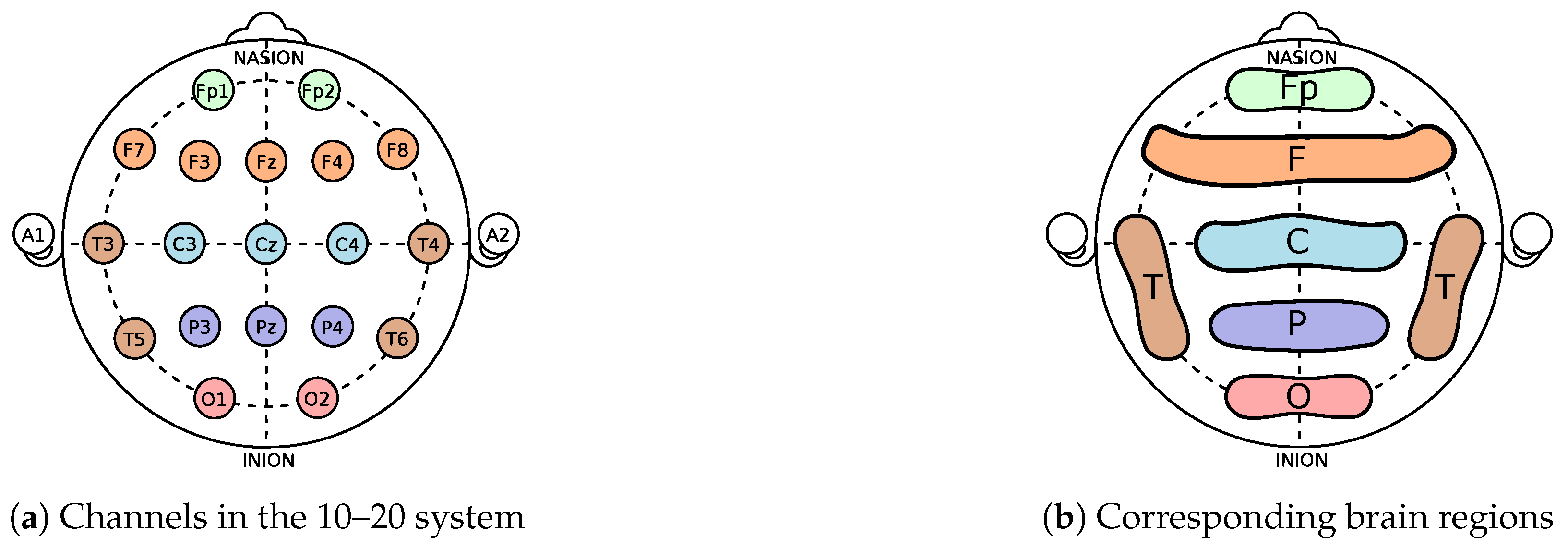
As data collection in the aforementioned study followed the International 10/20 scheme, 19 time series were obtained for every subject, each pertaining a different channel and thus capturing electrical activity in a distinct brain part. Auditory channels were disregarded as they were used for referencing purposes. Instead of using all available signals, in this paper, we use only six TSs for one patient, each one representing the average electric tension for each brain region: central C (C3, Cz, and C4), frontal F (F7, F3, Fz, F4, and F8), pre-frontal Fp (Fp1 and Fp2), occipital O (O1 and O2), parietal P (P3, P4, and Pz), and temporal T (T3, T4, T5, and T6). Please refer to Figure 1 for a graphical representation of this organisation.

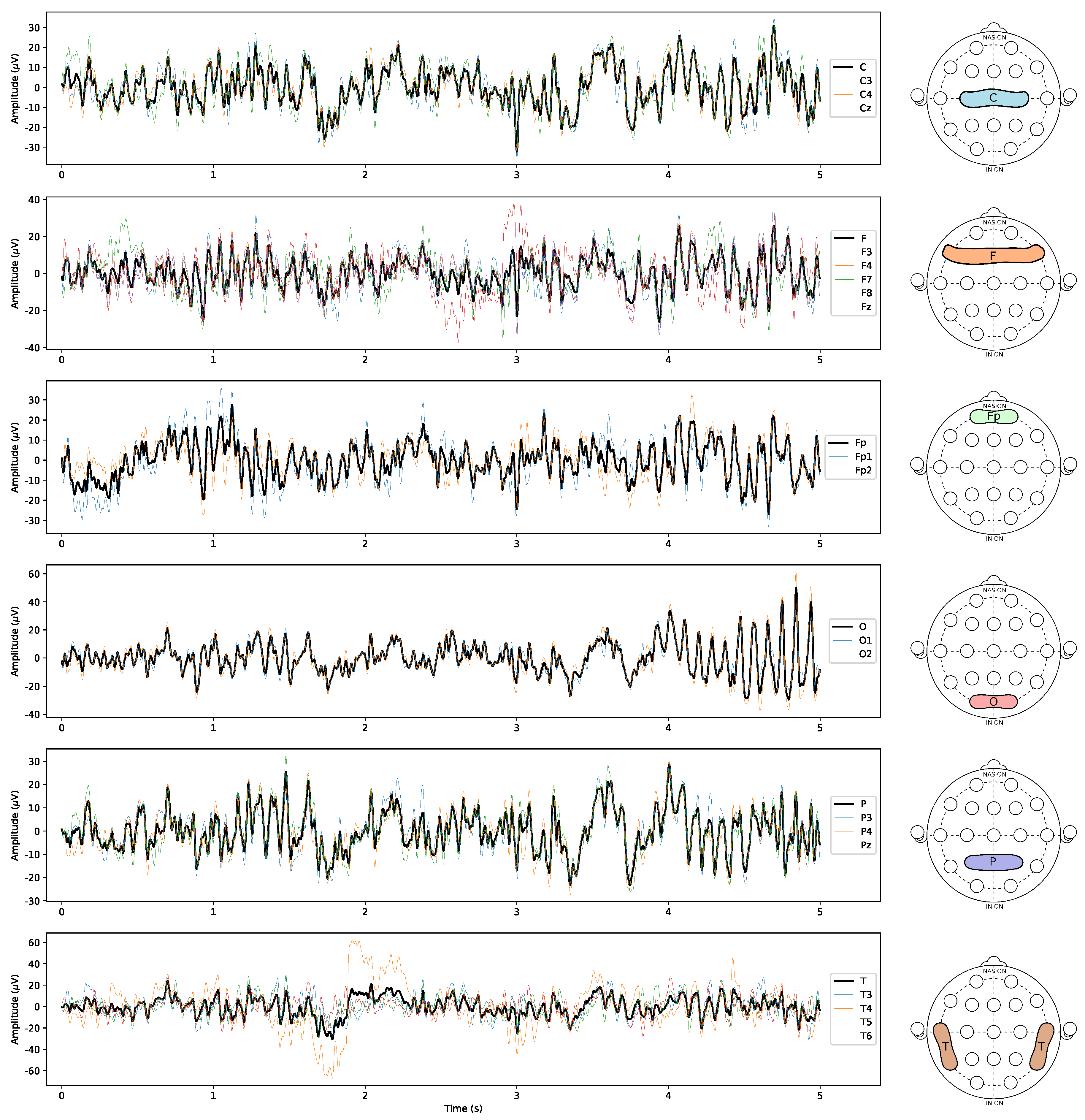
In summary, each of the 36 subjects is represented by 6 time series (each pertaining to an average of the multichannel signals, as illustrated in Figure 1) for each dataset (rest and activity), totalling 432 time series analysed in the paper.The TS dynamics of the aforesaid averages of each channel are presented for a representative subject in Figure 2. More details regarding the EEG records can be found in the original study in which they were collected [73].

3. Proposed Methods

This section briefly presents the methods that were used in the EEG analysis conducted in this paper, both in the frequency domain (the PSD approach, in Section 3.1) and in the time domain (the ARFIMA, DFA, and fractal dimensions, from Section 3.2 to Section 3.4).

3.1. Welch’s Power Spectral Density

Power spectral densities (PSDs) are widely used in signal processing and describe the energy density or power spectral of a signal according to a determined frequency range [48]. In the case of EEG signals, this tool can transform complex time series into directly interpretable information that can be categorised according to frequency bands and brain waves [75]. In summary, Welch’s method [69] partitions the data into smaller segments and computes a widowed discrete Fourier transform (DFT) at a determined frequency for each segment. A complete description of the method can be found in [49].

3.2. ARIMA and ARFIMA Models

In the investigation concerning the time-domain aspect of the EEG time series, we employ the ARFIMA(p,d,q) model, where $p\in N$ is the order (number of time lags) of the autoregressive model, $d\in R$ is the amount of times that past values are subtracted from the data (i.e., the degree of differencing), and $q\in N$ is the order of the moving-average model. In summary, the ARFIMA(p,d,q) [67] is a generalisation of the classical ARIMA(p,d,q) model, where the difference parameter d admits both integer and noninteger values.

Consider the integration of the series $Y_t$ along with a process that combines an auto-regressive (AR), an integrated (I), and a moving average (MA). One can express the ARIMA(p,d,q) with discrepancy operator (B) as

$$\varphi \left(B\right){(1-B)}^d{Y}_t=\mathsf{\Theta }\left(B\right){\epsilon }_t,$$

(1)

where $\varphi \left(B\right)$ = $1-{\phi }_{1}B-\dots -{\phi }_p{B}^p$ and $\mathsf{\Theta }\left(B\right)$ = $1+{\theta }_{1}B+\dots +{\theta }_q{B}^q$ are, respectively, the autoregressive and moving average operators, while ${\epsilon }_t$ is white noise. In order to expand the model to ARFIMA, the parameter d is modified to also assume noninteger values [76].

The ARFIMA(p,d,q) model is capable of capturing the dynamics processes with long-range dependency [76], with a general expression [67,77] defined by

$$\mathsf{\Phi }\left(B\right)y_t=\mathsf{\Theta }\left(B\right){(1-B)}^{-d}{\epsilon }_t,$$

(2)

where once again $\mathsf{\Phi }\left(B\right)=1-{\phi }_{1}B-\dots -{\phi }_p{B}^p$ and $\mathsf{\Theta }\left(B\right)=1+{\theta }_{1}B+\dots +{\theta }_q{B}^q$ are the autoregressive and moving average operators and ${\epsilon }_t$ describes white noise. It is important to highlight that functions $\mathsf{\Phi }\left(B\right)$ and $\mathsf{\Theta }\left(B\right)$ have no common roots, that B is the backward shift operator, and that ${(1-B)}^{-d}$ is the fractional differencing operator given by the following binomial expression [77]:

$${(1-B)}^{-d}=\sum _{j=0}^{\infty }\frac{\Gamma (j+d)}{\Gamma (j+1)T\left(d\right)}{B}^j=\sum _{j=0}^{\infty }{n}_j{B}^j,$$

(3)

where $\Gamma$ is the Gamma function.

One can describe an asymptotic approximation of $n_j$ with

$$n_j=\frac{\Gamma (j+d)}{\Gamma (j+d)\Gamma \left(d\right)}.$$

(4)

In this paper, the ARFIMA model we employ is a means to conduct the DFA of the EEG time series.

3.3. Detrented Fluctuation Analysis (DFA)

As previously discussed, TS concerning human or biosystems potentially have features that reach beyond local dependence [55] and the H index is often used as a means to quantify such dependence [78,79]. The Hurst exponent was introduced by H. E. Hurst [70] and is related to the concept of Brownian motion (Bm) and fractional Brownian motion (fBm).

In summary, the main properties concerning the H index [70,80] are the following:

(a)

0 < H < 1;

(b)

H = 1/2, for a random walk (Bm). The TS does not present a long memory process;

(c)

H > 1/2, for a persistent (long memory or correlated) process. This leads to the concept of the fBm; and

(d)

H < 1/2, for an anti-persistent (short-term memory, anti-correlated) process.

In a nutshell, if H is closer to 1, the probability of the next change being positive if the last change was also positive (i.e., persistent) is higher. One can use many approaches to find H, such as the classical rescaled range analysis originally developed in [81,82], the Fourier Analysis using the FFT algorithm [83,84], and the Detrented Fluctuation Analysis [85,86]. The DFA method avoids the spurious detection of correlation or apparent self-similarity and is capable of evaluating nonstationary series. The DFA involves successive steps to calculate H. The first step [85,87] consists in the following estimation

$$P\left(i\right)=\sum _{i=1}^N(P_t-P),$$

(5)

where N is the number of observations in the TS, $P_t$ represents the value (in this case, electrical tension) observed in time instant t, and P denotes the arithmetic average of this value.

Next, one [85,87] calculates the quantity $F\left(n\right)$ by means of the least squares method:

$$F\left(n\right)=\sqrt{\frac{1}{N}\sum _{i=1}^N{[P\left(i\right)-P_n\left(i\right)]}^2},$$

(6)

in which the trend is removed through the subtraction of the ordinary value $P_n\left(i\right)$ from $P\left(i\right)$.

The process is then repeated, and the slope curve relating $logF\left(n\right)$ with $log\left(n\right)$ determines the scaling H exponent. If the $kth$ order auto-covariance is defined as

$$\gamma \left(k\right)=Covariance[P_t,P_t+k],$$

(7)

then the $kth$ order autocorrelation can be found by using the following equation:

$$\rho =\frac{\gamma \left(k\right)}{\sqrt{Var\left(P_t\right)}\sqrt{Var(P_t+k)}}=\frac{\gamma \left(k\right)}{\gamma \left(0\right)}.$$

(8)

An important relation [88] between H and the autocorrelation function $\rho$ is drawn by

$$\rho =2^{2H-1}-1.$$

(9)

Concerning this relation, the decay speed of the autocorrelation function is also related to the H exponent [88] by

$$H=1/2+d,$$

(10)

where d is the fractional differencing parameter of the corresponding ARFIMA(p,d,q) model.

In Section 4.2, we apply H as a tool to investigate the possible trends in the EEG behaviour of patients.

3.4. Fractal Dimension

The fractal dimension D functions as a measure of local memory of the TS, where $1<\mathit{D}\le$ 2 for univariate series. In addition, the fractal dimension is connected to the long-term memory of a TS so that $\mathit{D}+\mathit{H}=2$, translating a perfect reflection from local (fractal dimension) to global behaviour (long-term memory) [89].

We can also summarise the properties of D [89,90] in TS pertaining to the following conditions: (i) $1<\mathit{D}\le 2$; (ii) $\mathit{D}=1.5$, which characterises TS as a random walk (Bm) phenomenon; (iii) $\mathit{D}<1.5$ indicates a persistent (long memory or correlated) process, leading to the definition of the fBm; and (iv) $\mathit{D}>1.5$ signalises anti-persistent processes (short-term memory, anti correlated).

In this paper, we adopt the Hall–Wood (HW) and Robust–Genton estimators [72,91] to obtain D.

3.4.1. Hall–Wood Estimator

The HW method [92] originates from a box-counting estimator considering small scales. In this approach, the boxes take into account not only their summations but also the areas under the curves. Formally, if one considers a scale ${ϵ}_l=l/n$, where $l=1,2,3,\dots n$, the area becomes

$$\widehat{A}(l/n)=(l/n)\sum _{i=1}^{[n/l]}(x_{il/n}-x_{(i-1)l/n}),$$

(11)

where $[n/l]$ is the integer part of $n/l$.

Hence, the HW estimator is defined as

$${\widehat{D}}_{HW}=2-\left(\sum _{i=1}^L(s_i-\overline{s})log\left(\widehat{A}(l/n)\right)\right){\left(\sum _{i=1}^L{(s_i-\overline{s})}^2\right)}^{-1},$$

(12)

where $L\ge 2$, $s_l=log(l/n)$, and $\overline{s}=(1/L){\sum }_{i=1}^L{s}_i$. In order to avoid bias, Hall and Wood suggested using $L=2$ [92], which entails

$${\widehat{D}}_{HW}=2-\frac{log\left(\widehat{A}(2/n)\right)-log\left(\widehat{A}(l/n)\right)}{log\left(2\right)}.$$

(13)

3.4.2. Robust–Genton Estimator

The RG method consists of a moments estimator of scales, as originally described in [91]. However, said approach is often considered a nonrobust method. In order to circumvent this problem, we herein consider the robust estimator implemented by Genton [91,93]. The calculations are given by

$$\widehat{V_2}(l/n)=\frac{1}{2(l-n)}\sum _{i=l}^n{(X_{i/n}-X_{(i-l)/n})}^2.$$

(14)

Similar to the HW method, one can obtain the RG estimator with the following equation:

$${\widehat{D}}_{RG}=2-\frac{1}{2}\left(\sum _{i=1}^L(s_i-\overline{s})log(\widehat{V_2}(l/n)\right){\left(\sum _{i=1}^L{(s_i-\overline{s})}^2\right)}^{-1},$$

(15)

where $L\ge 2$, $s_l=log(l/n)$ and $\overline{s}=(1/L){\sum }_{i=1}^L{s}_i$. Analogously, we can use $L=2$ to overcome bias drawbacks, thus obtaining

$${\widehat{D}}_{RG}=2-\frac{log\left(\widehat{V_2}(2/n)\right)-log\left(\widehat{V_2}(l/n)\right)}{2log\left(2\right)}.$$

(16)

4. Results and Discussion

This section presents the main results of the analyses conducted in this paper. We first present the PSD estimations in Section 4.1, comparing the activity and rest datasets and the performance groups in light of the brain wave categories. Next, in Section 4.2, we explore a statistical analysis of the results from the fractal approaches for the same datasets and comparisons.

4.1. Power Spectral Density Analysis

All PSD estimations and any graphical tools involving spectral density presented in this subsection were implemented by means of the Scipy and Matplotlib Libraries in Python with generally standard configurations. The sampling frequency was adopted at 500 Hz, chosen in accordance with the original signal. The frequencies herein considered were between 0.5 and 45 Hz since this was the range established by the cut-off filters in the original EEG data.

4.1.1. Comparison between Activity and Rest

The first batch of results compares the average of the PSD estimations for all 36 subjects categorised according to brain region, as presented in each subplot graph of Figure 3. The two curves in each graph describe the brain activity for the subjects while they were undertaking mental tasks and while at rest. As the axes for each graph are all scaled equally, one can see that regions O and P seem to show greater electrical activity in low-frequency ranges, with noticeable peaks for the 10 Hz mark in all brain regions. As for differences between the two curves, although they seem very close, it is worth highlighting that these are semi-log graphs, indicating that the y-axis is on the log scale. Hence, although visually subtle, the differences might be significant.

In this context, Figure 4 presents the same data content as Figure 3 but scaled individually and categorised according to frequency bands pertaining the basic brain waves described in [75], namely the theta (for frequencies between 4 and 8 Hz), alpha (8–12 Hz range), beta (12–35 Hz range), and gamma (35–45 Hz range) bands. Considering the space restrictions, we omitted the delta band (0.5–4 Hz range) in this figure since it is the less relevant frequency range for this study (since it mainly describes sleep and dreaming states).

Through the improved visualisation in Figure 4, one can see that, in general, there is a distinct shift in the prevalence of rest and activity curves as frequencies increase. It is possible to notice that, while the subjects are at rest, they have a higher prevalence of alpha brain waves. This could be expected as these waves are related to brain states in which the subjects are very relaxed with a passive attention (a plausible state for the rest dataset). On the other hand, this trend changes with higher frequencies, as it seems that the subjects present a higher number of beta and gamma waves while in activity. Indeed, those waves concern brain states involving an active mind and problem solving, which agrees with the arithmetic tasks undertaken by the subjects.

As a complementary visual device on the same data, Figure 5 presents the spectrogram of frequencies against time for subjects while performing arithmetic tasks (left) and at rest (right side). In general, we can infer the same conclusions as from Figure 3 with a few new perceptions. For all brain regions, the activity set shows a power peak around the 45 s mark even though the study design exposed in [73] does not specify if anything remarkable occurred at this time-point. The plots describing the T (temporal) region are the ones with most easily noticeable vertical lines, indicating frequent synchronous increases in the power of the signal, particularly in the activity data.

4.1.2. Comparison between Performance Groups

The next test aimed to identify differences in the EEG signal of subjects that obtained good, average, or bad performances in the arithmetic tasks. The 36 subjects were then ranked according to the number of correct subtractions they achieved during the tests and divided into subgroups with 12 participants each, with the name of the subgroups reflecting the patients’ performances. For more information regarding this division, please refer to Table A1. Following the same design choices regarding scales and organisation as in Section 4.1.1, Figure 6 and Figure 7 present the average PSD for these three groups organised according to brain region and frequency band (in the latter figure).

While the interpretation of Figure 6 and Figure 7 are less straight-forward than the rest/activity comparisons, one can identify some trends. In this analysis, we mainly consider the subplots pertaining to beta and gamma bands since we are concerned with the subjects’ performance and those frequencies pertaining to the brain areas related to concentration and problem solving. In addition, there seems to be some clear differences between curves when considering the gamma waves. In general, the curve regarding good performers is usually below the others, especially considering this higher-frequency range. The poor performers’ curves are mostly the highest in the beta band (with peaks around the 29 Hz mark) while the average ones are higher in the gamma range. In summary, these trends could indicate that poor and average performers might need more concentration (and brain effort) to deal with subtraction tasks when compared with good performers, thus generating more EEG activity in higher frequencies. In the work published with this original EEG data [73], the authors also imply that this seems to be the case.

4.2. Time-Domain Analysis and Fractal Indexes

In this subsection, we examine the time-domain analysis of the EGG signals, aiming to extract information oblivious to the PSD results. The indexes calculated, namely the differentiation order, the Hurst index, and the Hall–Wood and the Robust–Genton fractal dimensions, are graphically presented in Figure 8 and Figure 9 for all six brain regions studied in the paper. While the first figure presents the indexes for brain regions C, F, and Fp, the second shows regions O, P, and T. One might notice that the indexes are presented by means of pairs of plots, where data from the activity dataset are on the left and data pertaining to subjects at rest are on the right side.

One can observe that the results are visually very similar amid regions and even between rest and activity for most subjects, especially for indexes $D_{RG}$ and $D_{HW}$. On the other hand, d and H seem to be more volatile among subjects. These trends are confirmed with the mean and deviation values for the indexes, which are summarised in

Table 1. Information on the differentiation order, Hurst index, and Hall–Wood and Robust–Genton fractal dimensions for the EEG signals of the 35 subjects during activity.

Region	${\mathit{d}}_{\mathit{MIN}}$	${\mathit{d}}_{\mathit{MAX}}$	$\overline{\mathit{d}}$	${\mathit{\sigma }}_{\mathit{d}}$	${\mathit{H}}_{\mathit{MIN}}$	${\mathit{H}}_{\mathit{MAX}}$	$\overline{\mathit{H}}$	${\mathit{\sigma }}_{\mathit{H}}$	${\widehat{\overline{\mathit{D}}}}_{\mathit{HW}}$	${\mathit{\sigma }}_{\mathit{HW}}$	${\widehat{\overline{\mathit{D}}}}_{\mathit{RG}}$	${\mathit{\sigma }}_{\mathit{RG}}$
Indexes for subjects at rest
O	$0.0052$	$0.5000$	$0.0557$	$0.0835$	$0.2712$	$0.3574$	$0.3144$	$0.0171$	$1.0131$	$0.0051$	$1.0134$	$0.0051$
P	$0.0052$	$0.1910$	$0.0360$	$0.0325$	$0.2926$	$0.3592$	$0.3234$	$0.0160$	$1.0132$	$0.0038$	$1.0134$	$0.0040$
F	$0.0006$	$0.1288$	$0.0424$	$0.0294$	$0.2818$	$0.3682$	$0.3249$	$0.0225$	$1.0162$	$0.0039$	$1.0162$	$0.0040$
Fp	$0.0013$	$0.1379$	$0.0465$	$0.0304$	$0.2539$	$0.4743$	$0.3288$	$0.0432$	$1.0195$	$0.0051$	$1.0194$	$0.0050$
C	$0.0001$	$0.4845$	$0.0612$	$0.0994$	$0.2886$	$0.3701$	$0.3272$	$0.0170$	$1.0152$	$0.0037$	$1.0152$	$0.0037$
T	$0.0123$	$0.3110$	$0.0516$	$0.0563$	$0.2930$	$0.3737$	$0.3275$	$0.0179$	$1.0183$	$0.0056$	$1.0182$	$0.0056$
Indexes for subjects during activity
O	$0.0058$	$0.3808$	$0.0734$	$0.0924$	$0.2536$	$0.4310$	$0.3130$	$0.0283$	$1.0175$	$0.0111$	$1.0176$	$0.0112$
P	$0.0001$	$0.4982$	$0.0764$	$0.1191$	$0.2885$	$0.3771$	$0.3207$	$0.0197$	$1.0182$	$0.0122$	$1.0181$	$0.0118$
F	$0.0082$	$0.3911$	$0.0671$	$0.0860$	$0.2819$	$0.4202$	$0.3320$	$0.0328$	$1.0207$	$0.0117$	$1.0206$	$0.0114$
Fp	$0.0111$	$0.3536$	$0.0651$	$0.0636$	$0.2233$	$0.4806$	$0.3398$	$0.0614$	$1.0236$	$0.0094$	$1.0235$	$0.0090$
C	$0.0000$	$0.4668$	$0.0498$	$0.0790$	$0.2954$	$0.3857$	$0.3267$	$0.0214$	$1.0193$	$0.0110$	$1.0191$	$0.0108$
T	$0.0073$	$0.4704$	$0.0888$	$0.1208$	$0.2418$	$0.3857$	$0.3183$	$0.0298$	$1.0239$	$0.0147$	$1.0234$	$0.0143$

.

4.2.1. Statistical Comparison between Activity and Rest

In order to test if the indexes are statistically different for the activity and rest datasets, we conducted a Shapiro–Wilk normality test [94] with a significance level of 95% for the signals pertaining to each brain region. According to the results seen in

Table 2. Normality test for time series averages of every brain region considering the sets at activity and rest. A significance level of 95% (p-value < 0.05) rejects the null hypothesis of normality.

Shapiro–Wilk Normality Test: Activity vs. Rest Sets
	$\overline{\mathit{D}}$		$\mathit{H}$		${\mathit{D}}_{\mathit{HW}}$		${\mathit{D}}_{\mathit{RG}}$
Region	W	p-Value	W	p-Value	W	p-Value	W	p-Value
O	$5.84\times {10}^{-1}$	$5.65\times {10}^{-10}$	$8.76\times {10}^{-1}$	$3.74\times {10}^{-3}$	$7.20\times {10}^{-1}$	$2.07\times {10}^{-7}$	$1.75\times {10}^{-1}$	$1.81\times {10}^{-7}$
P	$4.99\times {10}^{-1}$	$2.82\times {10}^{-14}$	$9.71\times {10}^{-1}$	$9.89\times {10}^{-2}$	$5.61\times {10}^{-1}$	$2.38\times {10}^{-10}$	$5.78\times {10}^{-1}$	$4.59\times {10}^{-10}$
F	$5.64\times {10}^{-1}$	$2.64\times {10}^{-10}$	$9.60\times {10}^{-1}$	$2.08\times {10}^{-2}$	$5.92\times {10}^{-1}$	$7.77\times {10}^{-10}$	$5.99\times {10}^{-1}$	$1.01\times {10}^{-9}$
Fp	$6.84\times {10}^{-1}$	$3.71\times {10}^{-8}$	$9.76\times {10}^{-1}$	$1.88\times {10}^{-1}$	$8.05\times {10}^{-1}$	$2.30\times {10}^{-8}$	$8.09\times {10}^{-1}$	$3.04\times {10}^{-5}$
C	$4.85\times {10}^{-1}$	$1.76\times {10}^{-11}$	$9.58\times {10}^{-1}$	$1.66\times {10}^{-2}$	$5.71\times {10}^{-1}$	$3.44\times {10}^{-10}$	$5.67\times {10}^{-1}$	$3.02\times {10}^{-10}$
T	$5.86\times {10}^{-1}$	$6.01\times {10}^{-10}$	$9.45\times {10}^{-1}$	$3.53\times {10}^{-3}$	$6.31\times {10}^{-1}$	$3.70\times {10}^{-12}$	$6.20\times {10}^{-1}$	$2.32\times {10}^{-9}$

, in general, the time series failed the normality test, with two exceptions regarding the Hurst index for regions P and Fp.

Next, we conducted a variance analysis applying ANOVA–Tukey’s HSD and a Kruskal–Wallis–Dunn’s tests based on the normality tests for each time series. The results of this statistical analysis are presented in

Table 3. Variance analysis between the activity and rest sets for every brain region. A significance level of 95% ($p<0.05$) rejects the null hypothesis that the pairs are statistically equal.

ANOVA–Tukey’s HSD/Kruskal–Wallis–Dunn’s Tests: Activity vs. Rest Sets
	$\overline{\mathit{D}}$		$\mathit{H}$		${\mathit{D}}_{\mathit{HW}}$		${\mathit{D}}_{\mathit{RG}}$
Region	Z	p-Value	Mean Difference	p-Value	Z	p-Value	Z	p-Value
O	$-8.62\times {10}^{-1}$	$3.89\times {10}^{-1}$	$\phantom{-}4.28\times {10}^{-1}$	$6.69\times {10}^{-1}$	$-1.82\times {10}^{-0}$	$6.84\times {10}^{-2}$	$-1.76\times {10}^{-0}$	$7.83\times {10}^{-2}$
P	$-9.52\times {10}^{-1}$	$3.41\times {10}^{-1}$	$-2.69\times {10}^{-3}$	$5.31\times {10}^{-1}$	$-2.47\times {10}^{-0}$	$1.36\times {10}^{-2}$	$-2.45\times {10}^{-0}$	$1.45\times {10}^{-2}$
F	$-1.07\times {10}^{-0}$	$2.84\times {10}^{-1}$	$-5.52\times {10}^{-1}$	$5.81\times {10}^{-1}$	$-2.30\times {10}^{-0}$	$2.15\times {10}^{-2}$	$-2.29\times {10}^{-0}$	$2.19\times {10}^{-2}$
Fp	$-1.19\times {10}^{-0}$	$2.32\times {10}^{-1}$	$\phantom{-}1.11\times {10}^{-2}$	$3.86\times {10}^{-1}$	$-2.13\times {10}^{-0}$	$3.34\times {10}^{-2}$	$-2.15\times {10}^{-0}$	$3.15\times {10}^{-2}$
C	$\phantom{-}7.55\times {10}^{-1}$	$4.50\times {10}^{-1}$	$\phantom{-}6.59\times {10}^{-1}$	$5.10\times {10}^{-1}$	$-2.14\times {10}^{-0}$	$3.21\times {10}^{-2}$	$-2.12\times {10}^{-0}$	$3.36\times {10}^{-2}$
T	$-1.03\times {10}^{-0}$	$3.03\times {10}^{-1}$	$\phantom{-}1.66\times {10}^{-0}$	$9.78\times {10}^{-2}$	$-1.95\times {10}^{-0}$	$5.10\times {10}^{-2}$	$-1.81\times {10}^{-0}$	$7.01\times {10}^{-2}$

. Overall, the results cannot provide assertive statistical information differentiating the activity and rest datasets based on d and H indexes. On the other hand, $D_{HW}$ and $D_{RG}$ were capable of setting apart both datasets for most brain regions. A visual analysis of this statistical test is conducted in Section 4.2.4.

4.2.2. Statistical Comparison between Performance Groups

In this subsection, we investigate if a statistical difference between performance groups can be identified from the fractal measures calculated from the EEG activity dataset. Analogous to the procedure followed in Section 4.2.1, we conducted a Shapiro–Wilk normality test [94] with a significance level of 95% considering only the signals of said dataset. According to the results seen in

Table 4. Normality test for time series averages of every brain region considering the sets during activity. A significance level of 95% (p-value < $0.05$) rejects the null hypothesis of normality.

Shapiro–Wilk Normality Test: Activity Sets
	$\overline{\mathit{D}}$		$\mathit{H}$		${\mathit{D}}_{\mathit{HW}}$		${\mathit{D}}_{\mathit{RG}}$
Region	W	p-Value	W	p-Value	W	p-Value	W	p-Value
O	$6.45\times {10}^{-1}$	$4.28\times {10}^{-5}$	$8.29\times {10}^{-1}$	$6.55\times {10}^{-2}$	$7.06\times {10}^{-1}$	$3.52\times {10}^{-4}$	$7.03\times {10}^{-1}$	$3.16\times {10}^{-4}$
P	$5.77\times {10}^{-1}$	$5.31\times {10}^{-9}$	$9.54\times {10}^{-1}$	$1.39\times {10}^{-1}$	$5.66\times {10}^{-1}$	$3.83\times {10}^{-6}$	$5.74\times {10}^{-1}$	$4.80\times {10}^{-6}$
F	$5.66\times {10}^{-1}$	$3.88\times {10}^{-9}$	$9.49\times {10}^{-1}$	$1.00\times {10}^{-1}$	$6.06\times {10}^{-1}$	$1.28\times {10}^{-5}$	$5.95\times {10}^{-1}$	$9.14\times {10}^{-6}$
Fp	$6.60\times {10}^{-1}$	$7.00\times {10}^{-5}$	$9.73\times {10}^{-1}$	$4.98\times {10}^{-1}$	$7.83\times {10}^{-1}$	$7.63\times {10}^{-3}$	$7.91\times {10}^{-1}$	$1.08\times {10}^{-2}$
C	$4.78\times {10}^{-1}$	$3.59\times {10}^{-7}$	$9.18\times {10}^{-1}$	$1.09\times {10}^{-2}$	$5.74\times {10}^{-1}$	$4.89\times {10}^{-6}$	$5.58\times {10}^{-1}$	$3.09\times {10}^{-6}$
T	$6.26\times {10}^{-1}$	$2.35\times {10}^{-5}$	$9.53\times {10}^{-1}$	$1.29\times {10}^{-1}$	$6.16\times {10}^{-1}$	$1.72\times {10}^{-5}$	$5.97\times {10}^{-1}$	$9.65\times {10}^{-6}$

, in general, the time series failed the normality test, with exceptions once again regarding the Hurst index, in which the series are normal for all brain regions but C.

The variance analysis applying ANOVA–Tukey’s HSD and a Kruskal–Wallis–Dunn’s tests based on the normality tests for each time series are presented in

Table 5. Variance analysis between good, average, and poor performers for every brain region. A significance level of 95% ($p<0.05$) rejects the null hypothesis that the pairs are statistically equal.

ANOVA–Tukey’s HSD/Kruskal–Wallis–Dunn’s Tests: Performance Comparisons
	$\overline{\mathit{D}}$		$\mathit{H}$		${\mathit{D}}_{\mathit{HW}}$		${\mathit{D}}_{\mathit{RG}}$
Region	Z	p-Value	Mean-Difference	p-Value	Z	p-Value	Z	p-Value
Good performers vs. Average performers
O	$\phantom{-}4.26\times {10}^{-1}$	$6.70\times {10}^{-1}$	$-1.05\times {10}^{-3}$	$9.95\times {10}^{-1}$	$\phantom{-}6.80\times {10}^{-2}$	$9.46\times {10}^{-1}$	$\phantom{-}2.33\times {10}^{-1}$	$8.16\times {10}^{-1}$
P	$\phantom{-}4.26\times {10}^{-1}$	$6.70\times {10}^{-1}$	$\phantom{-}1.08\times {10}^{-3}$	$9.90\times {10}^{-1}$	$-6.81\times {10}^{-2}$	$9.46\times {10}^{-1}$	$-1.46\times {10}^{-1}$	$8.84\times {10}^{-1}$
F	$\phantom{-}1.54\times {10}^{-0}$	$1.23\times {10}^{-1}$	$-5.90\times {10}^{-3}$	$9.06\times {10}^{-1}$	$-6.31\times {10}^{-1}$	$5.28\times {10}^{-1}$	$-3.89\times {10}^{-1}$	$6.97\times {10}^{-1}$
Fp	$\phantom{-}1.45\times {10}^{-0}$	$1.46\times {10}^{-1}$	$-2.42\times {10}^{-2}$	$6.22\times {10}^{-1}$	$-6.21\times {10}^{-1}$	$5.34\times {10}^{-1}$	$-6.59\times {10}^{-1}$	$5.10\times {10}^{-1}$
C	$-1.45\times {10}^{-1}$	$8.84\times {10}^{-1}$	$-7.46\times {10}^{-1}$	$4.56\times {10}^{-1}$	$-2.14\times {10}^{-1}$	$8.30\times {10}^{-1}$	$-4.87\times {10}^{-2}$	$9.61\times {10}^{-1}$
T	$\phantom{-}1.07\times {10}^{-1}$	$9.15\times {10}^{-1}$	$\phantom{-}1.18\times {10}^{-2}$	$6.09\times {10}^{-1}$	$-2.33\times {10}^{-1}$	$8.16\times {10}^{-1}$	$-1.94\times {10}^{-2}$	$9.85\times {10}^{-1}$
Good performers vs. Poor performers
O	$\phantom{-}1.14\times {10}^{-0}$	$2.53\times {10}^{-1}$	$\phantom{-}1.75\times {10}^{-2}$	$2.96\times {10}^{-1}$	$7.19\times {10}^{-1}$	$4.72\times {10}^{-1}$	$8.16\times {10}^{-1}$	$4.15\times {10}^{-1}$
P	$\phantom{-}1.55\times {10}^{-1}$	$8.77\times {10}^{-1}$	$\phantom{-}1.49\times {10}^{-2}$	$1.55\times {10}^{-1}$	$7.68\times {10}^{-1}$	$4.42\times {10}^{-1}$	$7.59\times {10}^{-1}$	$4.48\times {10}^{-1}$
F	$\phantom{-}1.10\times {10}^{-0}$	$2.69\times {10}^{-1}$	$\phantom{-}3.03\times {10}^{-3}$	$9.74\times {10}^{-1}$	$5.44\times {10}^{-1}$	$5.87\times {10}^{-1}$	$7.68\times {10}^{-1}$	$4.42\times {10}^{-1}$
Fp	$\phantom{-}1.34\times {10}^{-0}$	$1.81\times {10}^{-1}$	$-1.31\times {10}^{-2}$	$8.68\times {10}^{-1}$	$3.59\times {10}^{-1}$	$7.19\times {10}^{-1}$	$3.39\times {10}^{-1}$	$7.35\times {10}^{-1}$
C	$-7.56\times {10}^{-1}$	$4.49\times {10}^{-1}$	$-1.58\times {10}^{-0}$	$1.14\times {10}^{-1}$	$9.16\times {10}^{-1}$	$3.60\times {10}^{-1}$	$9.25\times {10}^{-1}$	$3.55\times {10}^{-1}$
T	$-5.72\times {10}^{-1}$	$5.68\times {10}^{-1}$	$\phantom{-}1.62\times {10}^{-2}$	$4.02\times {10}^{-1}$	$9.32\times {10}^{-1}$	$3.51\times {10}^{-1}$	$1.10\times {10}^{-0}$	$2.73\times {10}^{-1}$
Average performers vs. Poor performers
O	$\phantom{-}7.17\times {10}^{-1}$	$4.73\times {10}^{-1}$	$-1.85\times {10}^{-2}$	$2.56\times {10}^{-1}$	$6.51\times {10}^{-1}$	$5.15\times {10}^{-1}$	$5.83\times {10}^{-1}$	$5.60\times {10}^{-1}$
P	$-2.71\times {10}^{-1}$	$7.86\times {10}^{-1}$	$-1.38\times {10}^{-2}$	$1.99\times {10}^{-1}$	$8.36\times {10}^{-1}$	$4.03\times {10}^{-1}$	$9.05\times {10}^{-1}$	$3.66\times {10}^{-1}$
F	$-4.36\times {10}^{-1}$	$6.63\times {10}^{-1}$	$-8.93\times {10}^{-3}$	$7.98\times {10}^{-1}$	$1.17\times {10}^{-0}$	$2.40\times {10}^{-1}$	$1.16\times {10}^{-0}$	$2.47\times {10}^{-1}$
Fp	$-1.16\times {10}^{-1}$	$9.07\times {10}^{-1}$	$-1.10\times {10}^{-2}$	$9.05\times {10}^{-1}$	$9.81\times {10}^{-1}$	$3.27\times {10}^{-1}$	$9.98\times {10}^{-1}$	$3.18\times {10}^{-1}$
C	$-6.11\times {10}^{-1}$	$5.41\times {10}^{-1}$	$-8.33\times {10}^{-1}$	$4.05\times {10}^{-1}$	$1.13\times {10}^{-0}$	$2.58\times {10}^{-1}$	$9.73\times {10}^{-1}$	$3.30\times {10}^{-1}$
T	$-6.78\times {10}^{-1}$	$4.98\times {10}^{-1}$	$-4.33\times {10}^{-3}$	$9.35\times {10}^{-1}$	$1.16\times {10}^{-0}$	$2.44\times {10}^{-1}$	$1.12\times {10}^{-0}$	$2.64\times {10}^{-1}$

, organised by performance comparisons. The results obtained suggest that the measures of differencing order, the Hurst exponent, and fractional dimensions are similar for good, average, and bad performers in the datasets considered. Therefore, the results cannot provide assertive statistical information to whether one group was more successful than other based on solely the time-domain data herein considered.

4.2.3. Statistical Comparison between Brain Regions during Activity

Finally, we apply the same procedure conducted in the previous instances to analyse whether there are significant statistical changes between the behaviour of electrical activity in the different brain regions analysed. The results of the variance analysis with a significance level of 95% are presented in

Table 6. Variance analysis between brain regions for the activity set. A significance level of 95% ($p<0.05$) rejects the null hypothesis that the pairs are statistically equal.

ANOVA–Tukey’s HSD/Kruskal–Wallis–Dunn’s Tests: Comparison between Regions of Task Sets
	$\overline{\mathit{D}}$		$\mathit{H}$		${\mathit{D}}_{\mathit{HW}}$		${\mathit{D}}_{\mathit{RG}}$
Regions	Z	p-Value	Mean-Difference	p-Value	Z	p-Value	Z	p-Value
F-C	$-1.92\times {10}^{-0}$	$5.50\times {10}^{-2}$	$-2.24\times {10}^{-1}$	$8.22\times {10}^{-1}$	$-8.17\times {10}^{-1}$	$4.14\times {10}^{-1}$	$-8.57\times {10}^{-1}$	$3.91\times {10}^{-1}$
Fp-C	$-2.64\times {10}^{-0}$	$8.22\times {10}^{-3}$	$-2.95\times {10}^{-1}$	$7.68\times {10}^{-1}$	$-2.84\times {10}^{-0}$	$4.56\times {10}^{-3}$	$-2.97\times {10}^{-0}$	$3.02\times {10}^{-3}$
O-C	$-7.24\times {10}^{-1}$	$4.69\times {10}^{-1}$	$-7.07\times {10}^{-2}$	$9.44\times {10}^{-1}$	$-2.02\times {10}^{-0}$	$4.34\times {10}^{-2}$	$-2.11\times {10}^{-0}$	$3.50\times {10}^{-2}$
P-C	$-1.69\times {10}^{-0}$	$9.20\times {10}^{-2}$	$\phantom{-}2.21\times {10}^{-0}$	$2.74\times {10}^{-2}$	$\phantom{-}1.04\times {10}^{-0}$	$3.00\times {10}^{-1}$	$\phantom{-}8.90\times {10}^{-1}$	$3.73\times {10}^{-1}$
T-C	$\phantom{-}2.34\times {10}^{-1}$	$8.15\times {10}^{-1}$	$\phantom{-}2.43\times {10}^{-0}$	$1.51\times {10}^{-2}$	$\phantom{-}1.85\times {10}^{-0}$	$6.38\times {10}^{-2}$	$\phantom{-}1.75\times {10}^{-0}$	$8.06\times {10}^{-2}$
Fp-F	$\phantom{-}9.58\times {10}^{-1}$	$3.38\times {10}^{-1}$	$\phantom{-}2.50\times {10}^{-0}$	$1.24\times {10}^{-2}$	$\phantom{-}3.87\times {10}^{-0}$	$1.07\times {10}^{-4}$	$\phantom{-}3.86\times {10}^{-0}$	$1.15\times {10}^{-4}$
O-F	$-9.29\times {10}^{-1}$	$3.53\times {10}^{-1}$	$\phantom{-}1.01\times {10}^{-0}$	$3.11\times {10}^{-1}$	$\phantom{-}7.93\times {10}^{-1}$	$4.28\times {10}^{-1}$	$\phantom{-}6.81\times {10}^{-1}$	$4.96\times {10}^{-1}$
P-F	$\phantom{-}9.90\times {10}^{-1}$	$3.22\times {10}^{-1}$	$\phantom{-}1.24\times {10}^{-0}$	$2.16\times {10}^{-1}$	$\phantom{-}1.61\times {10}^{-0}$	$1.07\times {10}^{-1}$	$\phantom{-}1.54\times {10}^{-0}$	$1.24\times {10}^{-1}$
T-F	$\phantom{-}1.71\times {10}^{-0}$	$8.65\times {10}^{-2}$	$\phantom{-}1.31\times {10}^{-0}$	$1.91\times {10}^{-1}$	$\phantom{-}3.63\times {10}^{-0}$	$2.83\times {10}^{-4}$	$\phantom{-}3.65\times {10}^{-0}$	$2.65\times {10}^{-4}$
O-Fp	$\phantom{-}7.56\times {10}^{-1}$	$4.50\times {10}^{-1}$	$-1.19\times {10}^{-0}$	$2.33\times {10}^{-1}$	$-2.44\times {10}^{-1}$	$8.08\times {10}^{-1}$	$-2.09\times {10}^{-1}$	$8.35\times {10}^{-1}$
P-Fp	$-1.88\times {10}^{-0}$	$6.06\times {10}^{-2}$	$\phantom{-}1.19\times {10}^{-0}$	$2.33\times {10}^{-1}$	$-2.04\times {10}^{-0}$	$4.13\times {10}^{-2}$	$-2.12\times {10}^{-0}$	$3.44\times {10}^{-2}$
T-Fp	$\phantom{-}4.24\times {10}^{-2}$	$9.66\times {10}^{-1}$	$\phantom{-}1.42\times {10}^{-0}$	$1.57\times {10}^{-1}$	$-1.22\times {10}^{-0}$	$2.21\times {10}^{-1}$	$-1.26\times {10}^{-0}$	$2.08\times {10}^{-1}$
P-O	$\phantom{-}7.67\times {10}^{-1}$	$4.43\times {10}^{-1}$	$\phantom{-}1.49\times {10}^{-0}$	$1.37\times {10}^{-1}$	$\phantom{-}7.96\times {10}^{-1}$	$4.26\times {10}^{-1}$	$\phantom{-}8.50\times {10}^{-1}$	$3.95\times {10}^{-1}$
T-O	$-1.91\times {10}^{-1}$	$8.48\times {10}^{-1}$	$-1.01\times {10}^{-0}$	$3.10\times {10}^{-1}$	$-3.08\times {10}^{-0}$	$2.09\times {10}^{-3}$	$-3.01\times {10}^{-0}$	$2.65\times {10}^{-3}$
T-P	$-9.48\times {10}^{-1}$	$3.43\times {10}^{-1}$	$\phantom{-}1.78\times {10}^{-1}$	$8.59\times {10}^{-1}$	$-2.83\times {10}^{-0}$	$4.60\times {10}^{-3}$	$-2.80\times {10}^{-0}$	$5.16\times {10}^{-3}$

, where each region was compared bilaterally. The index $\overline{D}$ could only identify a statistical difference between regions Fp and C, while H found differences between P and C, between T and C, and between Fp and F. The analysis concerning $D_{HW}$ and $D_{RG}$ found equivalent results for the two indexes, where they were capable of finding differences between the following pairs of brain regions: Fp–C, O–C, Fp–F, T–F, P–Fp, T–O, and T–P.

4.2.4. Graphical Analysis of Results

In this subsection, we propose a graphical summary of the main results pertaining the statistical analyses conducted in Section 4.2 as a straightforward approach to visualising the main results presented in Table 3, Table 5 and Table 6. Figure 10a presents the number of times that each fractal measure could differentiate datasets according to activity (vs. rest), performance, and between brain regions. As previously discussed, no index could identify differences between good, average, and bad performers while only $D_{HW}$ and $D_{RG}$ were capable of setting apart rest and activity data. All indexes found differences between regions at least one time. Considering the data illustrated in Figure 10a, $D_{HW}$ and $D_{RG}$ should be the measures chosen to evaluate data in comparison with the other indexes.

Figure 10b illustrates the number of times each region was differentiated in comparison with the others. The colours indicate the fractal measures, and the numbers inside each column show the amount of times a determined index was able to set that specific brain region apart from another. Overall, Fp seems to be the most distinct region from the others, meaning that, in comparison with others, it could be a good choice to investigate the EEG data of patients undertaking mental tasks. On the other hand, O was the least differentiated brain region, potentially indicating that the electrical activity in its correspondent channels might not be suitable for the analysis conducted in this paper.

5. Conclusions

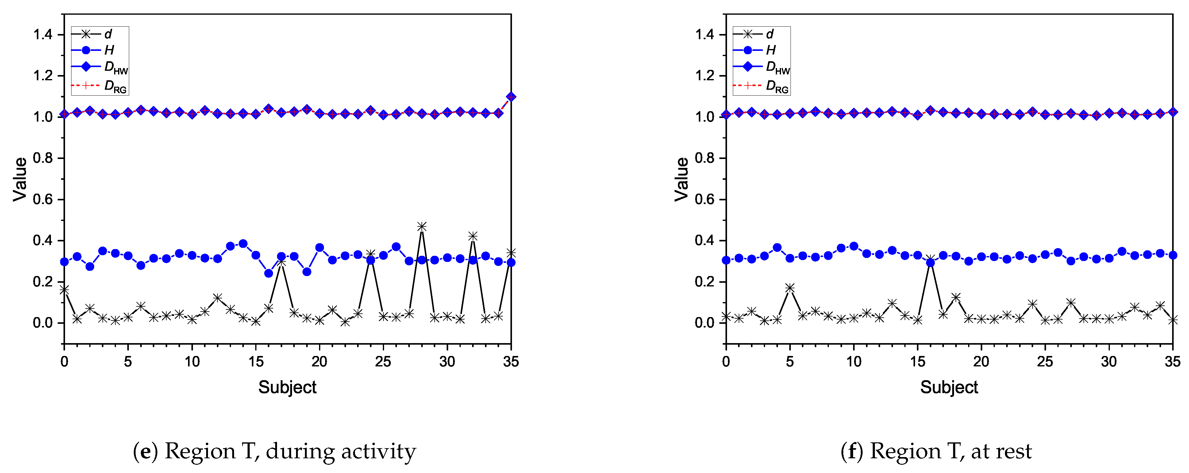
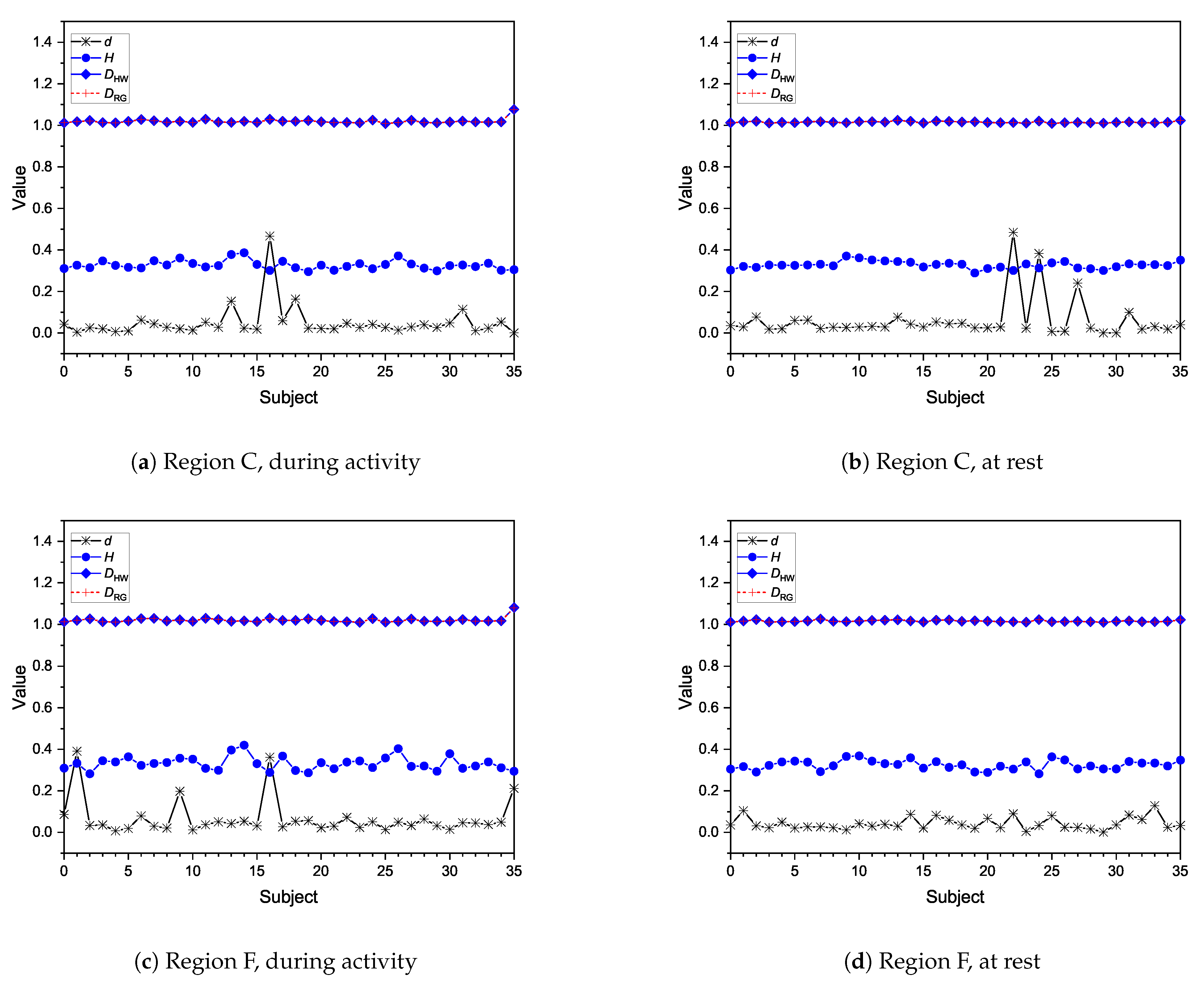
This study employed frequency- and time-based methods to explore extant EEG data in search of patterns that could differentiate signals of subjects undertaking a mental task (i) while at rest and during activity, (ii) in respect of how well the subjects performed during the arithmetic tests, and (iii) with spatial differences in the electrical activity in the brain. We chose to organise the EEG data for every patient into six time series, each corresponding to a brain region, which are averages according to the EEG channels in that area of the brain.

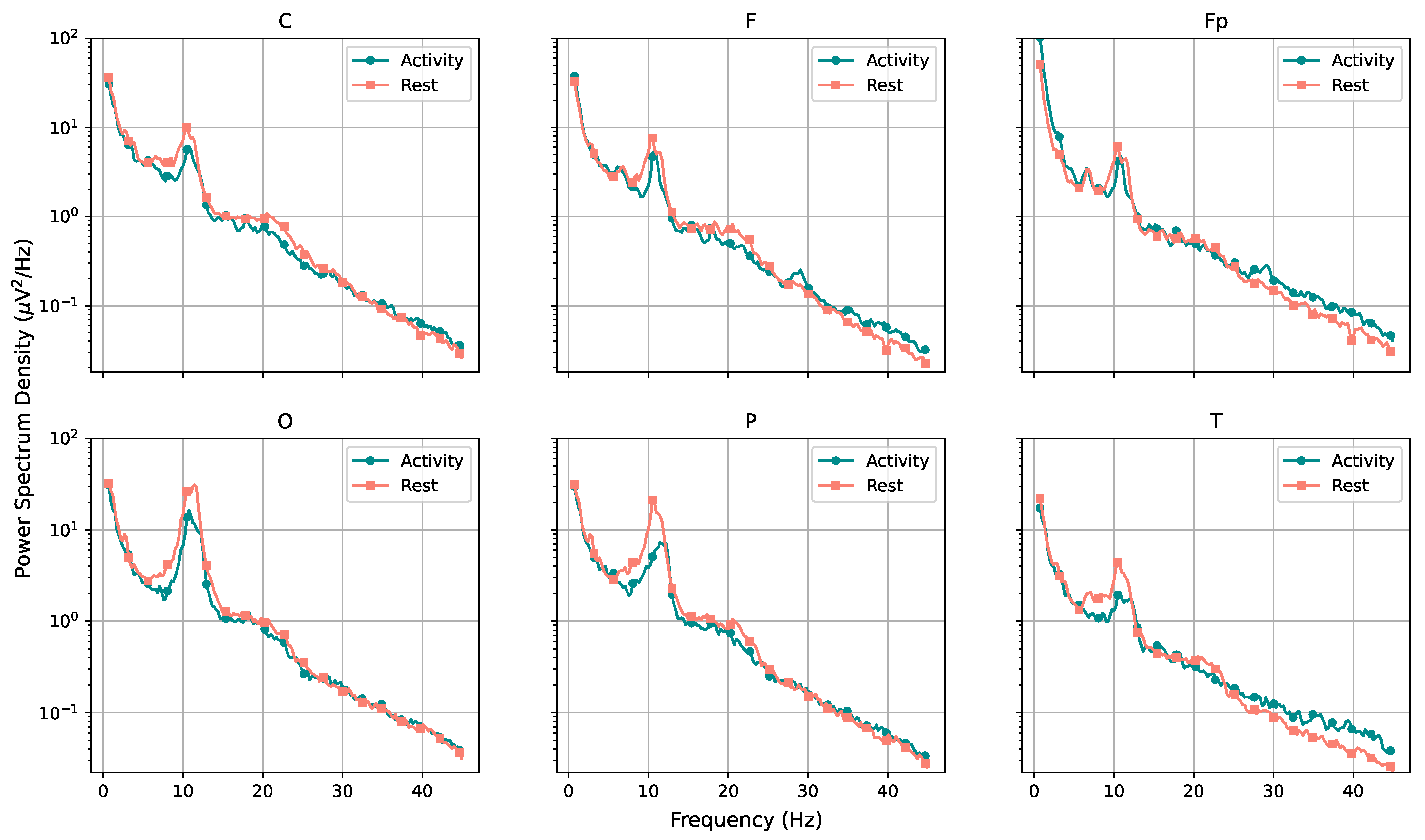
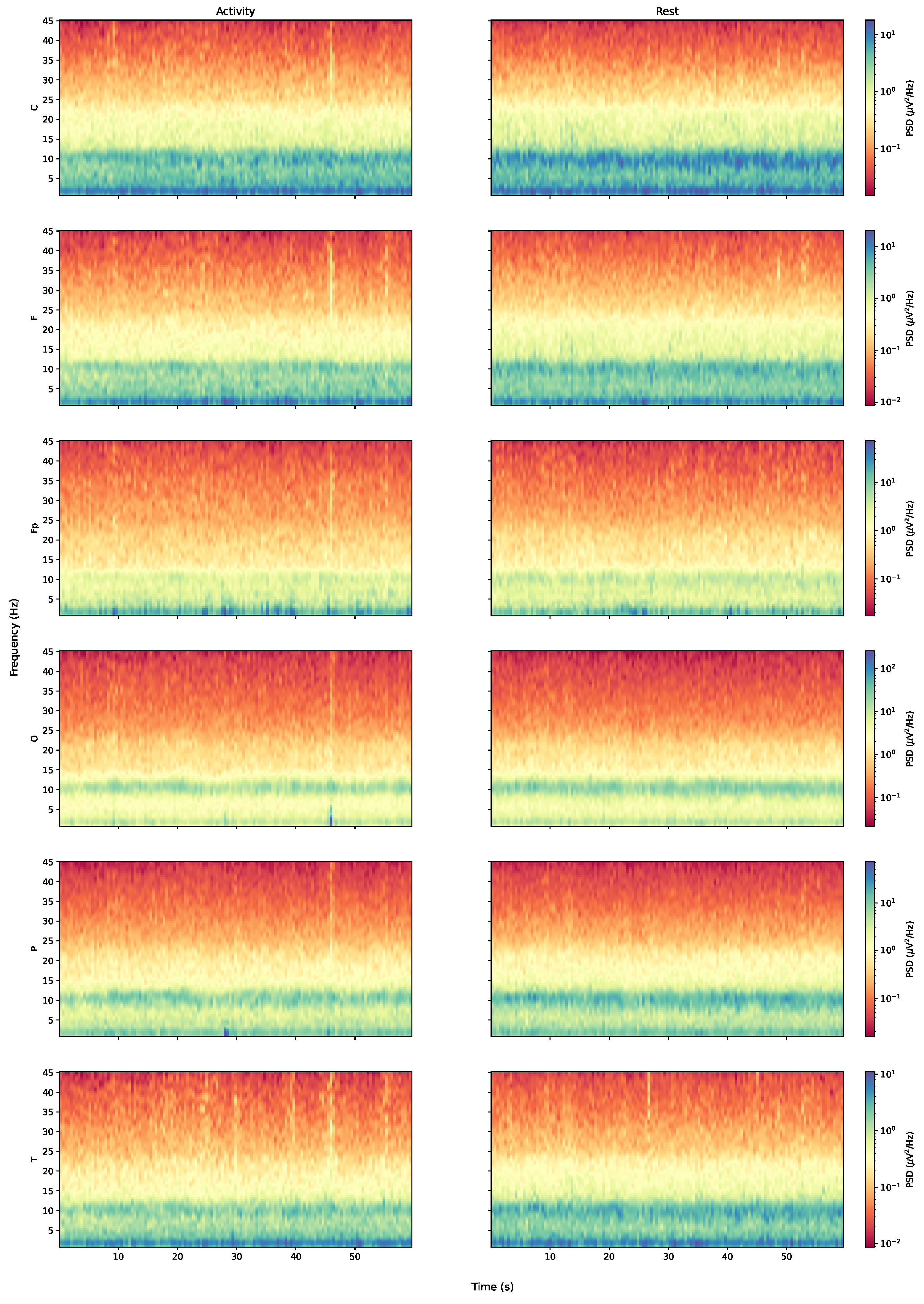
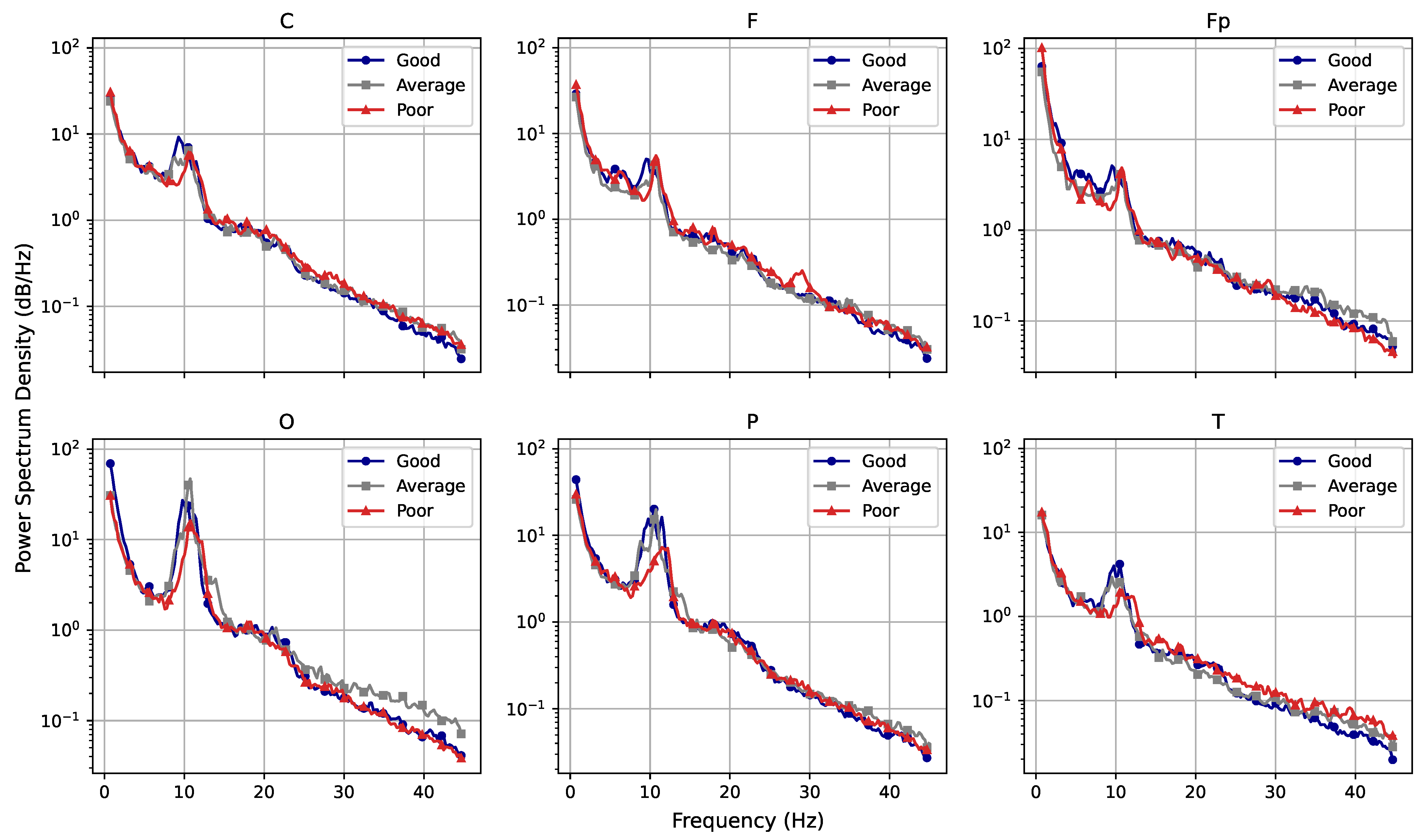
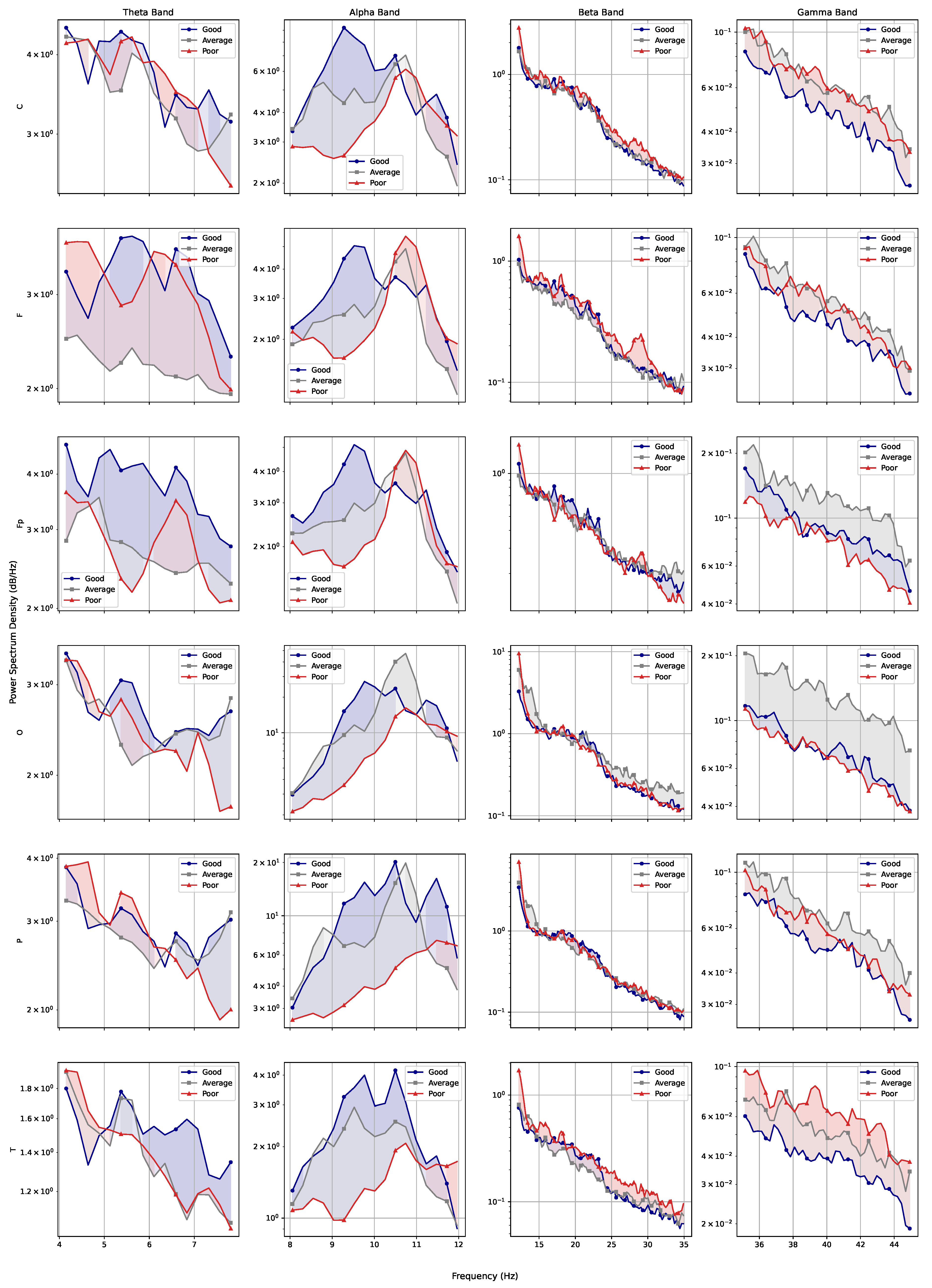
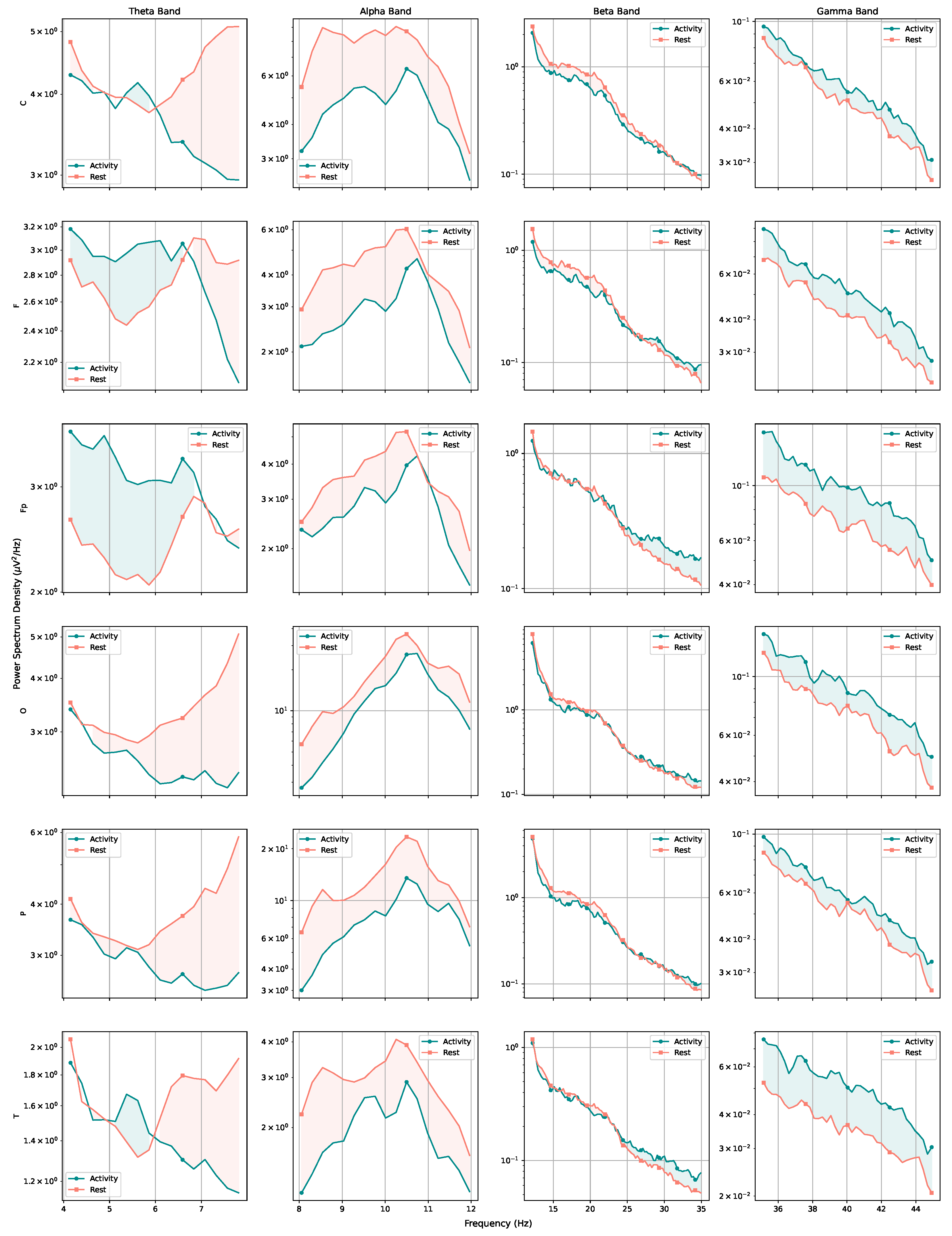
Considering the frequency domain, we estimated the power spectral density of the signals and found that, while the rest and activity datasets seem very close on a first analysis, the full picture changes when the amount of power pertaining each type of brain waves (theta, alpha, beta, and gamma) is considered. The results obtained through the estimations indicate that the subjects seem to have greater alpha-wave activity while at rest and increased gamma-wave activity while performing mental tasks. The spectrogram also reveals that the T region presents a larger number of synchronous frequency peaks when compared with other regions. The PSD curves for each region also indicated a few trends for performance curves, with average and poor performers apparently showing increased brain effort when compared with good performers (particularly when considering high-frequency ranges).

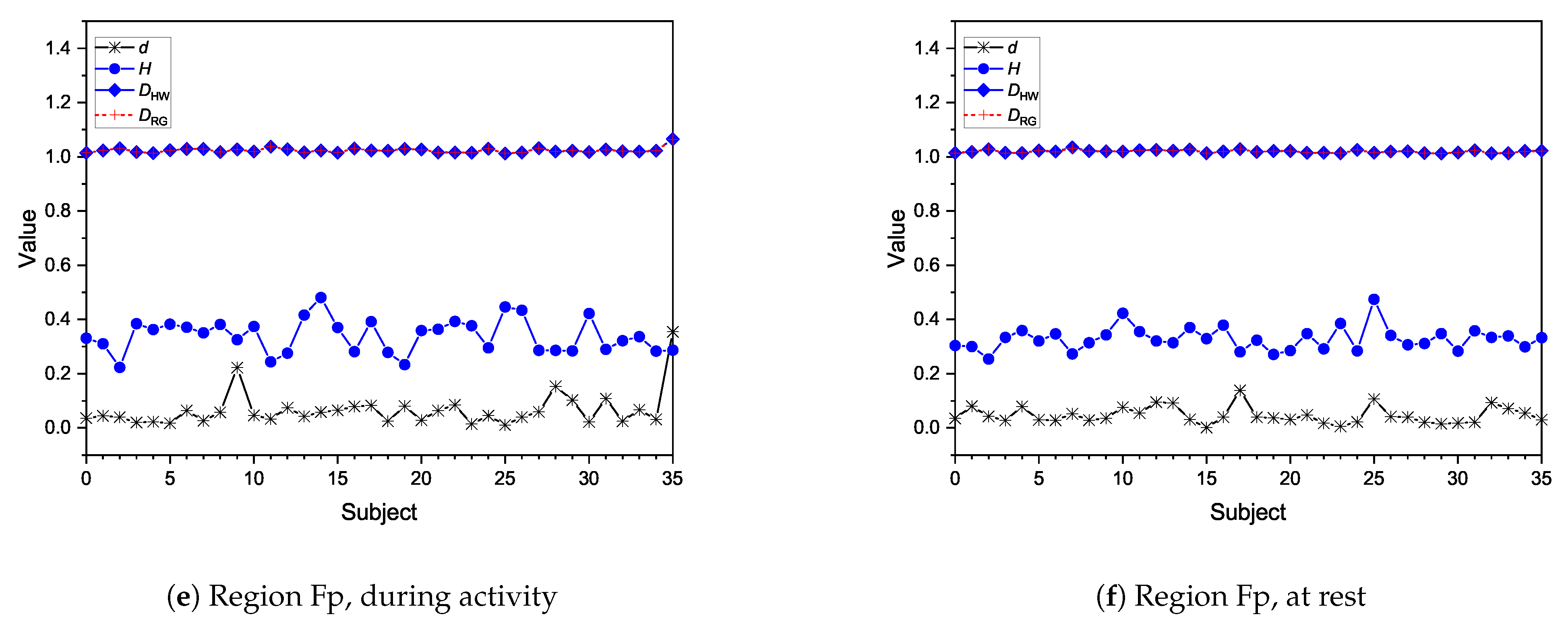
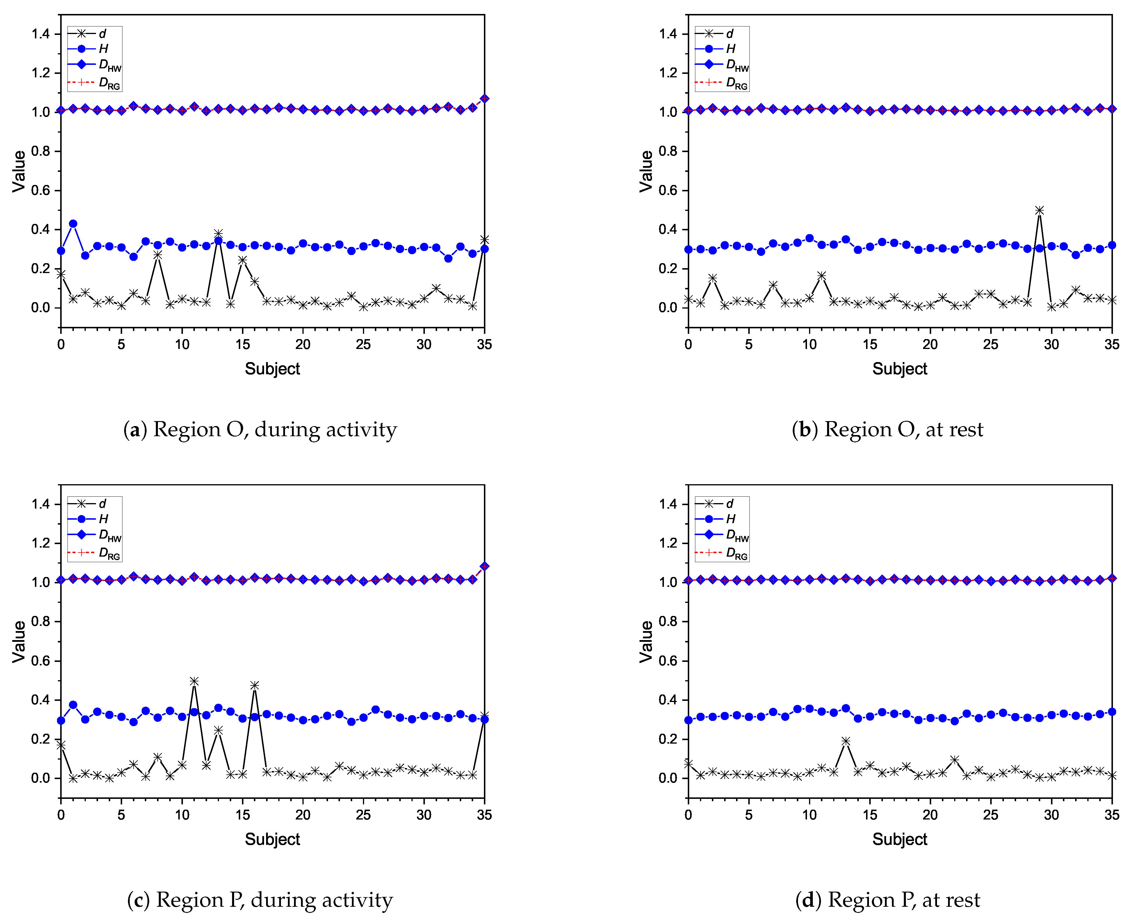
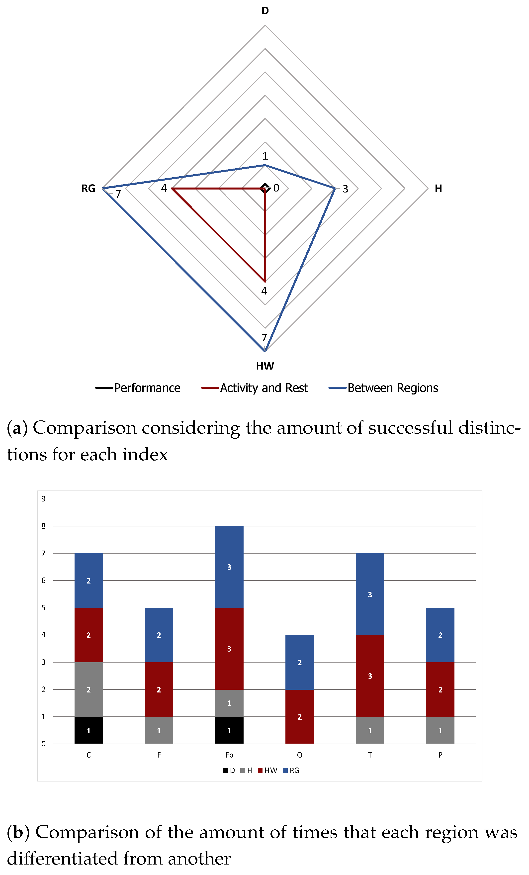
Moreover, fractional dimensions using the HW and RG estimators in addition to the H exponent by means of the DFA method were also explored. We adopted the Shapiro–Wilk normality test and variance analysis to assess if these indexes could offer any assertive statistical information regarding the three analyses in question. The aforementioned methods showed that the results achieved were very similar when comparing performance groups, with no statistical difference identified. As for differences between performance and brain regions, HW and RG estimators seemed to be better indicators. We also found that Fp seems to be the most differentiable brain region while O is the least differentiable, indicating that the former might be the most appropriate for analysing EEG data of patients undertaking mental tasks.

In conclusion, we believe that both frequency- and time-based methods were useful in the analysis and recommend that they should be used together in order to gain insights towards building a classifier of EEG data regarding mental tasks. In order to further investigate the matter and to exhaust related possibilities, in future work, we intend to explore some of the following options: (i) an analysis of the signals from other kinds of mental tasks; (ii) a consideration of the EEG channels individually (i.e., not using averages for each brain region); (iii) an extention of the number of mathematical tools, both within the scope of fractal dimensions as the frequency domain; (iv) the design of distinct analyses involving Lyapunov exponents applied to time series; and (v) the employment of machine learning approaches, such as deep learning and parametric models to extract features and to compare it with the results herein obtained.

References

1. Rideout, V.C. Mathematical and Computer Modeling of Physiological Systems; Prentice Hall: Englewood Cliffs, NJ, USA, 1991. [Google Scholar]
2. Debbouche, A.; Polovinkina, M.; Polovinkin, I.; Valentim, C.; David, S. On the stability of stationary solutions in diffusion models of oncological processes. Eur. Phys. J. Plus 2021, 136, 1–18. [Google Scholar] [CrossRef]
3. Valentim, C.A.; Rabi, J.A.; David, S.A.; Machado, J.A.T. On multistep tumor growth models of fractional variable-order. Biosystems 2021, 199, 104294. [Google Scholar] [CrossRef] [PubMed]
4. Lahmiri, S. Generalized Hurst exponent estimates differentiate EEG signals of healthy and epileptic patients. Phys. A Stat. Mech. Its Appl. 2018, 490, 378–385. [Google Scholar] [CrossRef]
5. Bhaduri, S.; Ghosh, D. Electroencephalographic data analysis with visibility graph technique for quantitative assessment of brain dysfunction. Clin. EEG Neurosci. 2015, 46, 218–223. [Google Scholar] [CrossRef] [PubMed]
6. Ghosh, D.; Dutta, S.; Chakraborty, S. Multifractal detrended cross-correlation analysis for epileptic patient in seizure and seizure free status. Chaos Solitons Fractals 2014, 67, 1–10. [Google Scholar] [CrossRef]
7. Frackowiak, R.S. Human Brain Function; Elsevier: Amsterdam, The Netherlands, 2004. [Google Scholar]
8. Sanei, S.; Chambers, J.A. EEG Signal Processing; John Wiley & Sons: Hoboken, NJ, USA, 2013. [Google Scholar]
9. Jayakar, P.; Gotman, J.; Harvey, A.S.; Palmini, A.; Tassi, L.; Schomer, D.; Dubeau, F.; Bartolomei, F.; Yu, A.; Kršek, P.; et al. Diagnostic utility of invasive EEG for epilepsy surgery: Indications, modalities, and techniques. Epilepsia 2016, 57, 1735–1747. [Google Scholar] [CrossRef]
10. David, S.A.; Cassela, C.I., Jr. Detrended fluctuation analysis and Hurst exponent as a measure to differentiate EEG signals. Biomath Commun. Suppl. 2018, 5. [Google Scholar]
11. Acharya, U.R.; Fujita, H.; Sudarshan, V.K.; Bhat, S.; Koh, J.E. Application of entropies for automated diagnosis of epilepsy using EEG signals: A review. Knowl.-Based Syst. 2015, 88, 85–96. [Google Scholar] [CrossRef]
12. Pellinen, J.; Carroll, E.; Friedman, D.; Boffa, M.; Dugan, P.; Friedman, D.E.; Gazzola, D.; Jongeling, A.; Rodriguez, A.J.; Holmes, M. Continuous EEG findings in patients with COVID-19 infection admitted to a New York academic hospital system. Epilepsia 2020, 61, 2097–2105. [Google Scholar] [CrossRef]
13. Miraglia, F.; Vecchio, F.; Bramanti, P.; Rossini, P.M. EEG characteristics in “eyes-open” versus “eyes-closed” conditions: Small-world network architecture in healthy aging and age-related brain degeneration. Clin. Neurophysiol. 2016, 127, 1261–1268. [Google Scholar] [CrossRef] [PubMed]
14. Canuet, L.; Ishii, R.; Pascual-Marqui, R.D.; Iwase, M.; Kurimoto, R.; Aoki, Y.; Ikeda, S.; Takahashi, H.; Nakahachi, T.; Takeda, M. Resting-state EEG source localization and functional connectivity in schizophrenia-like psychosis of epilepsy. PLoS ONE 2011, 6, e27863. [Google Scholar] [CrossRef] [PubMed] [Green Version]
15. Aboalayon, K.A.; Ocbagabir, H.T.; Faezipour, M. Efficient sleep stage classification based on EEG signals. In Proceedings of the IEEE Long Island Systems, Applications and Technology (LISAT) Conference 2014, Farmingdale, NY, USA, 2 May 2014; pp. 1–6. [Google Scholar]
16. Platt, B.; Riedel, G. The cholinergic system, EEG and sleep. Behav. Brain Res. 2011, 221, 499–504. [Google Scholar] [CrossRef]
17. Gibbs, S.A.; Proserpio, P.; Terzaghi, M.; Pigorini, A.; Sarasso, S.; Russo, G.L.; Tassi, L.; Nobili, L. Sleep-related epileptic behaviors and non-REM-related parasomnias: Insights from stereo-EEG. Sleep Med. Rev. 2016, 25, 4–20. [Google Scholar] [CrossRef] [PubMed] [Green Version]
18. Park, J.L.; Fairweather, M.M.; Donaldson, D.I. Making the case for mobile cognition: EEG and sports performance. Neurosci. Biobehav. Rev. 2015, 52, 117–130. [Google Scholar] [CrossRef] [Green Version]
19. Goodman, R.N.; Rietschel, J.C.; Lo, L.C.; Costanzo, M.E.; Hatfield, B.D. Stress, emotion regulation and cognitive performance: The predictive contributions of trait and state relative frontal EEG alpha asymmetry. Int. J. Psychophysiol. 2013, 87, 115–123. [Google Scholar] [CrossRef] [PubMed]
20. Johnson, R.R.; Popovic, D.P.; Olmstead, R.E.; Stikic, M.; Levendowski, D.J.; Berka, C. Drowsiness/alertness algorithm development and validation using synchronized EEG and cognitive performance to individualize a generalized model. Biol. Psychol. 2011, 87, 241–250. [Google Scholar] [CrossRef] [PubMed] [Green Version]
21. Sanyal, S.; Nag, S.; Banerjee, A.; Sengupta, R.; Ghosh, D. Music of brain and music on brain: A novel EEG sonification approach. Cogn. Neurodynamics 2019, 13, 13–31. [Google Scholar] [CrossRef] [PubMed]
22. Jaušovec, N.; Jaušovec, K. EEG activity during the performance of complex mental problems. Int. J. Psychophysiol. 2000, 36, 73–88. [Google Scholar] [CrossRef]
23. Lin, C.J.; Hsieh, M.H. Classification of mental task from EEG data using neural networks based on particle swarm optimization. Neurocomputing 2009, 72, 1121–1130. [Google Scholar] [CrossRef]
24. Wang, Q.; Sourina, O. Real-time mental arithmetic task recognition from EEG signals. IEEE Trans. Neural Syst. Rehabil. Eng. 2013, 21, 225–232. [Google Scholar] [CrossRef] [PubMed]
25. Müller-Putz, G.R.; Scherer, R.; Pfurtscheller, G.; Rupp, R. EEG-based neuroprosthesis control: A step towards clinical practice. Neurosci. Lett. 2005, 382, 169–174. [Google Scholar] [CrossRef]
26. del R Millan, J.; Mouriño, J.; Franzé, M.; Cincotti, F.; Varsta, M.; Heikkonen, J.; Babiloni, F. A local neural classifier for the recognition of EEG patterns associated to mental tasks. IEEE Trans. Neural Netw. 2002, 13, 678–686. [Google Scholar] [CrossRef] [Green Version]
27. Lotte, F.; Larrue, F.; Mühl, C. Flaws in current human training protocols for spontaneous brain-computer interfaces: Lessons learned from instructional design. Front. Hum. Neurosci. 2013, 7, 568. [Google Scholar] [CrossRef] [Green Version]
28. Acharya, U.R.; Molinari, F.; Sree, S.V.; Chattopadhyay, S.; Ng, K.H.; Suri, J.S. Automated diagnosis of epileptic EEG using entropies. Biomed. Signal Process. Control 2012, 7, 401–408. [Google Scholar] [CrossRef] [Green Version]
29. Yuan, Q.; Zhou, W.; Li, S.; Cai, D. Epileptic EEG classification based on extreme learning machine and nonlinear features. Epilepsy Res. 2011, 96, 29–38. [Google Scholar] [CrossRef] [PubMed]
30. Ruiz, R.A.S.; Ranta, R.; Louis-Dorr, V. EEG montage analysis in the blind source separation framework. Biomed. Signal Process. Control 2011, 6, 77–84. [Google Scholar] [CrossRef]
31. Coyle, D.; McGinnity, T.M.; Prasad, G. Improving the separability of multiple EEG features for a BCI by neural-time-series-prediction-preprocessing. Biomed. Signal Process. Control 2010, 5, 196–204. [Google Scholar] [CrossRef]
32. Ince, N.F.; Goksu, F.; Tewfik, A.H.; Arica, S. Adapting subject specific motor imagery EEG patterns in space–time–frequency for a brain computer interface. Biomed. Signal Process. Control 2009, 4, 236–246. [Google Scholar] [CrossRef]
33. Accardo, A.; Affinito, M.; Carrozzi, M.; Bouquet, F. Use of the fractal dimension for the analysis of electroencephalographic time series. Biol. Cybern. 1997, 77, 339–350. [Google Scholar]
34. Al-Nafjan, A.; Hosny, M.; Al-Ohali, Y.; Al-Wabil, A. Review and Classification of Emotion Recognition Based on EEG Brain-Computer Interface System Research: A Systematic Review. Appl. Sci. 2017, 7, 1239. [Google Scholar] [CrossRef] [Green Version]
35. Zhang, Y.; Zhang, S.; Ji, X. EEG-Based Classification of Emotions Using Empirical Mode Decomposition and Autoregressive Model. Multimed. Tools Appl. 2018, 77, 26697–26710. [Google Scholar] [CrossRef]
36. Pachori, R.B.; Sharma, R.; Patidar, S. Classification of Normal and Epileptic Seizure EEG Signals Based on Empirical Mode Decomposition. In Complex System Modelling and Control Through Intelligent Soft Computations; Zhu, Q., Azar, A.T., Eds.; Springer International Publishing: Cham, Switzerland, 2015; Volume 319, pp. 367–388. [Google Scholar]
37. Amin, H.U.; Mumtaz, W.; Subhani, A.R.; Saad, M.N.M.; Malik, A.S. Classification of EEG Signals Based on Pattern Recognition Approach. Front. Comput. Neurosci. 2017, 11, 103. [Google Scholar] [CrossRef] [Green Version]
38. Merlin Praveena, D.; Angelin Sarah, D.; Thomas George, S. Deep Learning Techniques for EEG Signal Applications—A Review. IETE J. Res. 2020, 1–8. [Google Scholar] [CrossRef]
39. Craik, A.; He, Y.; Contreras-Vidal, J.L. Deep Learning for Electroencephalogram (EEG) Classification Tasks: A Review. J. Neural Eng. 2019, 16, 031001. [Google Scholar] [CrossRef] [PubMed]
40. Oh, S.L.; Hagiwara, Y.; Raghavendra, U.; Yuvaraj, R.; Arunkumar, N.; Murugappan, M.; Acharya, U.R. A Deep Learning Approach for Parkinson’s Disease Diagnosis from EEG Signals. Neural Comput. Appl. 2020, 32, 10927–10933. [Google Scholar] [CrossRef]
41. Ullah, I.; Hussain, M.; Qazi, E.u.H.; Aboalsamh, H. An Automated System for Epilepsy Detection Using EEG Brain Signals Based on Deep Learning Approach. Expert Syst. Appl. 2018, 107, 61–71. [Google Scholar] [CrossRef] [Green Version]
42. Wu, E.Q.; Deng, P.Y.; Qiu, X.Y.; Tang, Z.; Zhang, W.M.; Zhu, L.M.; Ren, H.; Zhou, G.R.; Sheng, R.S.F. Detecting Fatigue Status of Pilots Based on Deep Learning Network Using EEG Signals. IEEE Trans. Cogn. Dev. Syst. 2021, 13, 575–585. [Google Scholar] [CrossRef]
43. Zeng, H.; Yang, C.; Dai, G.; Qin, F.; Zhang, J.; Kong, W. EEG Classification of Driver Mental States by Deep Learning. Cogn. Neurodynamics 2018, 12, 597–606. [Google Scholar] [CrossRef] [PubMed]
44. Tao, W.; Li, C.; Song, R.; Cheng, J.; Liu, Y.; Wan, F.; Chen, X. EEG-Based Emotion Recognition via Channel-Wise Attention and Self Attention. IEEE Trans. Affect. Comput. 2020. [Google Scholar] [CrossRef]
45. Gannouni, S.; Aledaily, A.; Belwafi, K.; Aboalsamh, H. Emotion Detection Using Electroencephalography Signals and a Zero-Time Windowing-Based Epoch Estimation and Relevant Electrode Identification. Sci. Rep. 2021, 11, 7071. [Google Scholar] [CrossRef] [PubMed]
46. Zheng, X.; Chen, W.; You, Y.; Jiang, Y.; Li, M.; Zhang, T. Ensemble Deep Learning for Automated Visual Classification Using EEG Signals. Pattern Recognit. 2020, 102, 107147. [Google Scholar] [CrossRef]
47. Varshney, A.; Ghosh, S.K.; Padhy, S.; Tripathy, R.K.; Acharya, U.R. Automated Classification of Mental Arithmetic Tasks Using Recurrent Neural Network and Entropy Features Obtained from Multi-Channel EEG Signals. Electronics 2021, 10, 1079. [Google Scholar] [CrossRef]
48. Youngworth, R.N.; Gallagher, B.B.; Stamper, B.L. An overview of power spectral density (PSD) calculations. In Optical Manufacturing and Testing VI; International Society for Optics and Photonics: San Diego, CA, USA, 2005; Volume 5869, p. 58690U. [Google Scholar]
49. Solomon, O.M., Jr. PSD Computations Using Welch’s Method. [Power Spectral Density (PSD)]; Technical report; Sandia National Labs: Albuquerque, NM, USA, 1991. [Google Scholar]
50. Demuru, M.; La Cava, S.M.; Pani, S.M.; Fraschini, M. A comparison between power spectral density and network metrics: An EEG study. Biomed. Signal Process. Control 2020, 57, 101760. [Google Scholar] [CrossRef]
51. Carrier, J.; Land, S.; Buysse, D.J.; Kupfer, D.J.; Monk, T.H. The effects of age and gender on sleep EEG power spectral density in the middle years of life (ages 20–60 years old). Psychophysiology 2001, 38, 232–242. [Google Scholar] [CrossRef] [PubMed]
52. Wang, R.; Wang, J.; Yu, H.; Wei, X.; Yang, C.; Deng, B. Power spectral density and coherence analysis of Alzheimer’s EEG. Cogn. Neurodynamics 2015, 9, 291–304. [Google Scholar] [CrossRef] [PubMed]
53. Glass, A.; Kwiatkowski, A. Power spectral density changes in the EEG during mental arithmetic and eye-opening. Psychol. Forsch. 1970, 33, 85–99. [Google Scholar] [CrossRef]
54. Hasan, M.J.; Shon, D.; Im, K.; Choi, H.K.; Yoo, D.S.; Kim, J.M. Sleep state classification using power spectral density and residual neural network with multichannel EEG signals. Appl. Sci. 2020, 10, 7639. [Google Scholar] [CrossRef]
55. Granger, C.W.; Joyeux, R. An introduction to long-memory time series models and fractional differencing. J. Time Ser. Anal. 1980, 1, 15–29. [Google Scholar] [CrossRef]
56. David, S.A.; Machado, J.; Trevisan, L.R.; Inácio, C., Jr.; Lopes, A.M. Dynamics of Commodities Prices: Integer and Fractional Models. Fundam. Inform. 2017, 151, 389–408. [Google Scholar] [CrossRef]
57. David, S.; Inácio, C., Jr.; Quintino, D.; Machado, J. Measuring the Brazilian ethanol and gasoline market efficiency using DFA-Hurst and fractal dimension. Energy Econ. 2020, 85, 104614. [Google Scholar] [CrossRef]
58. Ionescu, C.M. The Human Respiratory System: An Analysis of the Interplay between Anatomy, Structure, Breathing and Fractal Dynamics; Springer Science & Business Media: Cham, Switzerland, 2013. [Google Scholar]
59. Ionescu, C.M.; Copot, D. Monitoring respiratory impedance by wearable sensor device: Protocol and methodology. Biomed. Signal Process. Control 2017, 36, 57–62. [Google Scholar] [CrossRef]
60. Assadi, I.; Charef, A.; Copot, D.; De Keyser, R.; Bensouici, T.; Ionescu, C. Evaluation of respiratory properties by means of fractional order models. Biomed. Signal Process. Control 2017, 34, 206–213. [Google Scholar] [CrossRef]
61. Braeken, M.A.K.A.; Jones, A.; Otte, R.A.; Widjaja, D.; Van Huffel, S.; Monsieur, G.J.Y.J.; Van Oirschot, C.M.; den Bergh, B.R.H. Anxious women do not show the expected decrease in cardiovascular stress responsiveness as pregnancy advances. Biol. Psychol. 2015, 111, 83–89. [Google Scholar] [CrossRef]
62. Aubert, A.E.; Vandeput, S.; Beckers, F.; Liu, J.; Verheyden, B.; Van Huffel, S. Complexity of cardiovascular regulation in small animals. Philos. Trans. R. Soc. A Math. Phys. Eng. Sci. 2009, 367, 1239–1250. [Google Scholar] [CrossRef]
63. Mortier, E.; Struys, M.; De Smet, T.; Versichelen, L.; Rolly, G. Closed-loop controlled administration of propofol using bispectral analysis. Anaesthesia 1998, 53, 749–754. [Google Scholar] [CrossRef] [PubMed]
64. Jameson, L.C.; Sloan, T.B. Using EEG to monitor anesthesia drug effects during surgery. J. Clin. Monit. Comput. 2006, 20, 445–472. [Google Scholar] [CrossRef]
65. David, S.A.; Machado, J.A.T.; Inácio, C.M.; Valentim, C. A combined measure to differentiate EEG signals using fractal dimension and MFDFA-Hurst. Commun. Nonlinear Sci. Numer. Simul. 2020, 84, 105170. [Google Scholar] [CrossRef]
66. Fraschini, M.; Demuru, M.; Crobe, A.; Marrosu, F.; Stam, C.J.; Hillebrand, A. The effect of epoch length on estimated EEG functional connectivity and brain network organisation. J. Neural Eng. 2016, 13, 036015. [Google Scholar] [CrossRef] [PubMed]
67. Box, G.; Jenkins, G.M.; Reinsel, G. Time Series Analysis: Forecasting & Control; Prentice Hall: Upper Saddle River, NJ, USA, 1994. [Google Scholar]
68. Xu, L.; Ivanov, P.C.; Hu, K.; Chen, Z.; Carbone, A.; Stanley, H.E. Quantifying signals with power-law correlations: A comparative study of detrended fluctuation analysis and detrended moving average techniques. Phys. Rev. E 2005, 71, 051101. [Google Scholar] [CrossRef] [Green Version]
69. Welch, P.D. A direct digital method of power spectrum estimation. IBM J. Res. Dev. 1961, 5, 141–156. [Google Scholar] [CrossRef]
70. Hurst, H. The long-term dependence in stock returns. Trans. Am. Soc. Civ. Eng. 1951, 116, 77–99. [Google Scholar] [CrossRef]
71. Bryce, R.; Sprague, K. Revisiting detrended fluctuation analysis. Sci. Rep. 2012, 2, 315. [Google Scholar] [CrossRef] [Green Version]
72. Gneiting, T.; Ševčíková, H.; Percival, D.B. Estimators of fractal dimension: Assessing the roughness of time series and spatial data. Stat. Sci. 2012, 27, 247–277. [Google Scholar] [CrossRef]
73. Zyma, I.; Tukaev, S.; Seleznov, I.; Kiyono, K.; Popov, A.; Chernykh, M.; Shpenkov, O. Electroencephalograms during mental arithmetic task performance. Data 2019, 4, 14. [Google Scholar] [CrossRef] [Green Version]
74. Goldberger, A.; Amaral, L.; Glass, L.; Hausdorff, J.; Ivanov, P.; Mark, R.; Mietus, J.; Moody, G.; Peng, C.; Stanley, H. PhysioBank, PhysioToolkit, and PhysioNet: Components of a new research resource for complex physiologic signals. Circulation 2000, 101, e215–e220. [Google Scholar] [CrossRef] [PubMed] [Green Version]
75. Abhang, P.A.; Gawali, B.W.; Mehrotra, S.C. Chapter 2—Technological Basics of EEG Recording and Operation of Apparatus. In Introduction to EEG- and Speech-Based Emotion Recognition; Abhang, P.A., Gawali, B.W., Mehrotra, S.C., Eds.; Academic Press: Cambridge, MA, USA, 2016; pp. 19–50. [Google Scholar]
76. Baillie, R.T. Long memory processes and fractional integration in econometrics. J. Econom. 1996, 73, 5–59. [Google Scholar] [CrossRef]
77. Franco, G.C.; Reisen, V.A. Bootstrap approaches and confidence intervals for stationary and non-stationary long-range dependence processes. Phys. A Stat. Mech. Its Appl. 2007, 375, 546–562. [Google Scholar] [CrossRef]
78. Cizeau, P.; Liu, Y.; Meyer, M.; Peng, C.K.; Stanley, H.E. Volatility distribution in the S&P500 stock index. Phys. A Stat. Mech. Its Appl. 1997, 245, 441–445. [Google Scholar]
79. Ausloos, M.; Vandewalle, N.; Boveroux, P.; Minguet, A.; Ivanova, K. Applications of statistical physics to economic and financial topics. Phys. A Stat. Mech. Its Appl. 1999, 274, 229–240. [Google Scholar] [CrossRef]
80. Tarnopolski, M. On the relationship between the Hurst exponent, the ratio of the mean square successive difference to the variance, and the number of turning points. Phys. A Stat. Mech. Its Appl. 2016, 461, 662–673. [Google Scholar] [CrossRef] [Green Version]
81. Mandelbrot, B. Statistical methodology for nonperiodic cycles: From the covariance to R/S analysis. In Annals of Economic and Social Measurement; NBER: Cambridge, MA, USA, 1972; pp. 259–290. [Google Scholar]
82. Mandelbrot, B.B.; Wallis, J.R. Robustness of the rescaled range R/S in the measurement of noncyclic long run statistical dependence. Water Resour. Res. 1969, 5, 967–988. [Google Scholar] [CrossRef]
83. Welch, P. The use of fast Fourier transform for the estimation of power spectra: A method based on time averaging over short, modified periodograms. IEEE Trans. Audio Electroacoust. 1967, 15, 70–73. [Google Scholar] [CrossRef] [Green Version]
84. Roerink, G.J.; Menenti, M.; Verhoef, W. Reconstructing cloudfree NDVI composites using Fourier analysis of time series. Int. J. Remote Sens. 2000, 21, 1911–1917. [Google Scholar] [CrossRef]
85. Peng, C.K.; Buldyrev, S.V.; Havlin, S.; Simons, M.; Stanley, H.E.; Goldberger, A.L. Mosaic organization of DNA nucleotides. Phys. Rev. E 1994, 49, 1685–1689. [Google Scholar] [CrossRef] [Green Version]
86. Shieh, S.J. Long memory and sampling frequencies: Evidence in stock index futures markets. Int. J. Theor. Appl. Financ. 2006, 9, 787–799. [Google Scholar] [CrossRef]
87. Serinaldi, F. Use and misuse of some Hurst parameter estimators applied to stationary and non-stationary financial time series. Phys. A Stat. Mech. Its Appl. 2010, 389, 2770–2781. [Google Scholar] [CrossRef]
88. Peters, E.E. Chaos and Order in the Capital Markets: A New View of Cycles, Prices, and Market Volatility; John Wiley & Sons: Hoboken, NJ, USA, 1996; Volume 1. [Google Scholar]
89. Kristoufek, L.; Vosvrda, M. Measuring capital market efficiency: Global and local correlations structure. Phys. A Stat. Mech. Its Appl. 2013, 392, 184–193. [Google Scholar] [CrossRef] [Green Version]
90. Kristoufek, L. How are rescaled range analyses affected by different memory and distributional properties? A Monte Carlo study. Phys. A Stat. Mech. Its Appl. 2012, 391, 4252–4260. [Google Scholar] [CrossRef]
91. Genton, M.G. Variogram fitting by generalized least squares using an explicit formula for the covariance structure. Math. Geol. 1998, 30, 323–345. [Google Scholar] [CrossRef]
92. Hall, P.; Wood, A. On the performance of box-counting estimators of fractal dimension. Biometrika 1993, 80, 246–251. [Google Scholar] [CrossRef]
93. Ma, Y.; Genton, M.G. Highly Robust Estimation of the Autocovariance Function. J. Time Ser. Anal. 2000, 21, 663–684. [Google Scholar] [CrossRef]
94. Shapiro, S.S.; Wilk, M.B. An analysis of variance test for normality (complete samples). Biometrika 1965, 52, 591–611. [Google Scholar] [CrossRef]
Figure 1. Representation of the International 10–20 EEG scheme with a colour distinction for each average TS considered in this paper: C (C3, Cz, and C4), F (F7, F3, Fz, F4, and F8), Fp (Fp1 and Fp2), O (O1 and O2), P (P3, P4, and Pz), and T (T3, T4, T5, and T6). The reader can notice that each of the six averages corresponds to a specific brain region.
Fractalfract 05 00225 g001
Figure 2. Representation of the EEG TS of a random patient (Subject 00) during the mental task (activity dataset). For visualisation purposes, only the interval between 0 and 5 s is shown. Each subplot concerns one of the six brain areas presented in Figure 1. The black lines represent the average signal for each area, and the colored ones represent the original channel signals.
Fractalfract 05 00225 g002
Figure 3. Comparison of the power spectral density between the activity and rest datasets (considering the average for all 36 subjects).
Fractalfract 05 00225 g003
Figure 4. Comparison of the power spectral density between the activity and rest datasets (considering the average for all 36 subjects). Visualisation improved through individual scaling and frequency-band classification.
Fractalfract 05 00225 g004
Figure 5. Comparison of the spectrograms between activity (left) and rest (right) datasets (considering the average for all 36 subjects).
Fractalfract 05 00225 g005
Figure 6. Comparison of the power spectral density between good, average, and poor performers (considering the average for each group of 12 subjects).
Fractalfract 05 00225 g006
Figure 7. Comparison of the power spectral density between good, average, and poor performers (considering the average for each group of 12 subjects). Visualisation improved for each frequency band.
Fractalfract 05 00225 g007
Figure 8. Fractal measures comparing the activity (left) and rest (right) datasets for all 36 patients according to brain region: (a,b) region C, (c,d) region F, and (e,f) region Fp.
Fractalfract 05 00225 g008aFractalfract 05 00225 g008b
Figure 9. Fractal measures comparing the activity (left) and rest (right) datasets for all 36 patients according to brain region: (a,b) region O, (c,d) region P, and (e,f) region T.
Fractalfract 05 00225 g009aFractalfract 05 00225 g009b
Figure 10. Graphical representation of the findings concerning the statistical analysis conducted in Section 4.2.
Fractalfract 05 00225 g010