Asymptotics of Karhunen–Loève Eigenvalues for Sub-Fractional Brownian Motion and Its Application

Abstract

In the present paper, the Karhunen–Loève eigenvalues for a sub-fractional Brownian motion are considered. Rigorous large n asymptotics for those eigenvalues are shown, based on the functional analysis method. By virtue of these asymptotics, along with some standard large deviations results, asymptotical estimates for the small $L^2$-ball probabilities for a sub-fractional Brownian motion are derived. Asymptotic analysis on the Karhunen–Loève eigenvalues for the corresponding “derivative” process is also established.

1. Introduction

The eigenproblem for a centered stochastic process $X={\left(X\left(t\right)\right)}_{t\in [0,1]}$ over a probability space $(\Omega ,\mathcal{F},P)$ with covariance function $K(s,t)=\mathrm{E}\left[X\right(s\left)X\right(t\left)\right]$ consists of finding all pairs $(\lambda ,\phi )$ satisfying the equation

$$K\phi =\lambda \phi$$

(1)

in $L^2\left([0,1]\right)$, where the corresponding linear operator is defined by the following:

$$\left(K\phi \right)\left(t\right)\triangleq {\int }_0^{1}K(s,t)\phi \left(s\right)\mathrm{d}s,\forall t\in [0,1].$$

(2)

If $K(s,t)$ is square integrable, then $K:L^2\left([0,1]\right)\to L^2\left([0,1]\right)$ is self-adjoint, positive and compact. Hence, the eigenvalues $\left\{{\lambda }_n\right\}$ for the operator K are nonnegative and converge to zero after being arranged in decreasing order. The corresponding normalized eigenfunctions $\left\{{\phi }_n\right\}$ form a complete orthonormal basis in $L^2\left([0,1]\right)$.

In addition, if ${\left(X\left(t\right)\right)}_{t\in [0,1]}$ is a square-integrable process with zero mean and continuous covariance, there exists a Karhunen–Loève expansion(cf. [1]). More precisely, it admits a representation over $[0,1]$ as a uniformly $L^2(\Omega )$-convergent series:

$$X\left(t\right)=\sum _{n=0}^{\infty }\sqrt{{\lambda }_n}{\xi }_n{\phi }_n\left(t\right),$$

(3)

where $\left\{{\xi }_n\right\}$ are orthonormal (i.e., $\mathrm{E}\left[{\xi }_j{\xi }_k\right]={\delta }_{jk}$) random variables in $L^2(\Omega )$ with zero mean. Since the Karhunen–Loève expansion is an influential tool in analyzing the properties of stochastic processes, $\left\{{\lambda }_n\right\}$ are also called Karhunen–Loève eigenvalues for ${\left(X\left(t\right)\right)}_{t\in [0,1]}$.

There are many applications relevant to the eigenproblems for stochastic processes: asymptotics of the small ball probabilities(cf. [2]), sampling from heavy tailed distributions(cf. [3]) and so on.

On most occasions, such kinds of eigenvalues and eigenfunctions are notoriously hard to find explicitly. One exception is for the standard Brownian motion $B={\left(B_t\right)}_{t\in [0,1]}$, where

$${\lambda }_n=\frac{1}{{(n+1/2)}^2{\pi }^2}$$

(4)

and

$${\phi }_n\left(t\right)=\sqrt{2}sin(n+1/2)\pi t$$

(5)

hold for $n=0,1,2,\cdots$. This problem can be easily solved by reducing (1) to a simple boundary value problem for an ordinary differential equation (cf. [1]).

A widely used extension of Brownian motion is fractional Brownian motion $B^H={\left(B^H\left(t\right)\right)}_{t\in [0,1]}$. Its covariance function is as follows:

$$K^H(s,t)=\frac{1}{2}(s^{2H}+t^{2H}-{\left|s-t\right|}^{2H}),$$

(6)

where $H\in (0,1)$ is called its Hurst exponent. The case $H=\frac{1}{2}$ corresponds to Brownian motion. There are some important properties of fractional Brownian motion. For examples, it has self-similarity and stationary increments (cf. [4]). The eigenproblem of fractional Brownian motion is discussed in several papers (cf. [5,6]).

The author in [5] used the functional analysis method, and obtained the asymptotics of the eigenvalues for fractional Brownian motion. The following is just a rephrasing of one of his results:

Theorem 1

(J. C. Bronski, 2003). For the fractional Brownian motion with Hurst exponent $H\in (0,1)$, its Karhunen–Loève eigenvalues satisfy the following large n asymptotics:

$${\lambda }_n=\frac{sin\left(\pi H\right)\Gamma (2H+1)}{{\left(n\pi \right)}^{2H+1}}+o\left(n^{-\frac{(2H+2)(4H+3)}{4H+5}+\delta }\right)$$

(7)

for every $\delta >0$, where Γ denotes the usual Euler gamma function.

The authors in [6] converted the eigenproblem for fractional Brownian motion into an integro-algebraic system by using Laplace transform, and solved it by taking the inversion of the Laplace transform. Some other processes derived by Brownian motion, such as Brownian bridge (cf. [7]), the Ornstein–Uhlenbeck process (cf. [8]), etc., can be solved in a similar way. Compared to [5], the profile of the eigenpair analyzed with the method in [6] is more complete and accurate.

Similar to the fractional Brownian motion, the sub-fractional Brownian motion also presents the properties of self-similarity and long-range dependence (when the Hurst exponent $H>\frac{1}{2}$). Different from the fractional Brownian motion, there is an additional term ${|t+s|}^{2H}$ in its covariance, and the increment is not stationary as a result. From this point of view, it was expected that the idea in [6] could also work for sub-fractional Brownian motion. However, it seems that it does not work for sub-fractional Brownian motion because of the loss of some translation structure.

Consequently, the main results in this paper are based on the idea in [5]. It should be pointed out that there are some flaws in [5]. To some extent, the results (see Remark 2 in Section 5) in this paper are supplements and corrections of the ones in [5].

This paper is organized as follows. In the next section, the asymptotics of eigenvalues for sub-fractional Brownian motion and its derivative process are stated. As an application of those results, the small ball estimates for sub-fractional Brownian motion are presented in Section 3, but its proof is omitted since it is just a duplication of the one in [5]. Some technical lemmas are presented in Section 4. Section 5 concludes with the details of the proofs of the main results.

2. The Main Results

Sub-fractional Brownian motion(sfBm) $B_{sub}^H={\left(B_{sub}^H\left(t\right)\right)}_{t\in [0,1]}$ is a centered long-range dependence Gaussian process. Like fractional Brownian motion, its covariance function is as follows:

$$K_{sub}^H(s,t)=s^{2H}+t^{2H}-\frac{1}{2}{[(s+t)}^{2H}+{\left|s-t\right|}^{2H}]$$

(8)

with an exponent $H\in (0,1)$. The case $H=\frac{1}{2}$ also corresponds to Brownian motion. To some extent, sfBm is intermediate between Brownian motion and fractional Brownian motion (cf. [9]). This is reflected in the nonstationarity and correlation of the increments and the covariance of the non-overlapping intervals. The increments on non-overlapping intervals are more weakly correlated than fractional Brownian motion, and the covariance decays polynomially at a higher rate.

In this paper, the eigenproblems for the following two operators are studied:

$$\begin{array}{cc}\hfill \left(K_{sub}^H\phi \right)\left(t\right)& ={\int }_0^1(s^{2H}+t^{2H}-\frac{1}{2}{[(s+t)}^{2H}+{\left|s-t\right|}^{2H}\left]\right)\phi \left(s\right)\mathrm{d}s,\hfill \end{array}$$

(9)

$$\begin{array}{cc}\hfill \left({\tilde{K}}_{sub}^H\phi \right)\left(t\right)& ={\int }_0^1{H(2H-1)\left(\right|s-t|}^{2H-2}-{(s+t)}^{2H-2})\phi \left(s\right)\mathrm{d}s\hfill \end{array}$$

(10)

The operator in (9) for $H\in (0,1)$ is related to sfBm itself, and the one in (10) for $H\in (\frac{1}{2},1)$ corresponds to the formal derivative of the sfBm. In fact, the operator ${\tilde{K}}_{sub}^H$ determines the correlation structure of Wiener integrals of square-integrable deterministic functions through the following formula:

$$\mathrm{E}\left[{\int }_0^{1}f\mathrm{d}{B}_{sub}^H{\int }_0^{1}g\mathrm{d}{B}_{sub}^H\right]={\int }_0^{1}f\left(t\right)\left({\tilde{K}}_{sub}^{H}g\right)\left(t\right)\mathrm{d}t.$$

(11)

To the best of the authors’ knowledge, those eigenproblems have not been rigorously considered before. Borrowed the idea from [5], rough asymptotics of eigenvalues of sub-fractional Brownian motion are derived as follows.

Theorem 2.

The Karhunen–Loève eigenvalues of sub-fractional Brownian motion with exponent $H\in (0,1)$ satisfies the following:

• Case $0<H<\frac{-1+\sqrt{74}}{8}$:

  $${\lambda }_n=\frac{{\gamma }_H}{n^{2H+1}}+o\left(n^{-\frac{(2H+2)(4H+3)}{4H+5}+\delta }\right)$$

  (12)
  for every $\delta >0$ and $n\gg 1$;
• Case $\frac{-1+\sqrt{74}}{8}\le H<1$:

  $${\lambda }_n=\frac{{\gamma }_H}{n^{2H+1}}+O\left(n^{-3}\right)$$

  (13)

for every $n\gg 1$, where ${\gamma }_H=\frac{2sin\left(\pi H\right)\Gamma (2H+1)}{{\pi }^{2H+1}}$.

Specifically, given an orthonormal basis in $L^2\left([0,1]\right)$, the operator $K_{sub}^H$ in (9) over $L^2\left([0,1]\right)$ is of a representation as a linear operator over ${\ell }^2$, which is essentially an infinite-dimensional matrix. Asymptotic analysis on matrix elements is performed, based on some technical lemmas, some of which (see Lemma 3) are improvements of the ones in [5]. Afterward, Theorem 2 is obtained in terms of the theory of compact operators. However, the asymptotics in Theorem 2 are rough by simple observation or through numerical simulation, although the details of the simulation are not provided here.

Next, the conclusion is about the eigenvalues of the derivative process of sub-fractional Brownian. Unlike [6], the case $H\in (0,\frac{1}{2})$ is skipped.

Theorem 3.

The Karhunen–Loève eigenvalues of the derivative process of sub-fractional Brownian with $H\in (\frac{1}{2},1)$ satisfy the following:

$${\lambda }_n=\frac{{\kappa }_H}{n^{2H-1}}+o\left(n^{-\frac{2H(4H-1)}{4H+1}+\delta }\right)$$

(14)

for every $\delta >0$ and $n\gg 1$, where ${\kappa }_H=\frac{2sin\left(\pi H\right)\Gamma (2H+1)}{{\pi }^{2H-1}}$.

3. An Application: Small $L^2$-Ball Estimate

The small ball estimate is an interesting topic in probability theory, and also has important applications in statistical mechanic models. It yields estimates of the probability that some stochastic process $X={\left(X\left(t\right)\right)}_{t\in [0,1]}$ will lie inside a ball of radius $\epsilon$ in a certain given norm $\left|\right|·\left|\right|.$ As for the $L^2\left([0,1]\right)$-norm, if X is a centered Gaussian process with continuous covariance, there holds the following:

$${\left|\right|X\left|\right|}_{L^2}^2={\int }_0^{1}X{\left(t\right)}^2\mathrm{d}t=\sum _{n=0}^{\infty }{\lambda }_n{\xi }_n^2,$$

(15)

where $\left\{{\xi }_n\right\}$ are i.i.d. $N(0,1)$ random variables. As pointed out in [5], a crucial quantity to derive the small ball estimate for fractional Brownian motion is the following determinant:

$$D^H\left(\lambda \right)=\prod _{n=0}^{\infty }(1+2\lambda {\lambda }_n)$$

(16)

which is a variant of the Fredholm determinant of $K^H$.

Now, the small $L^2\left([0,1]\right)$-ball estimate of sfBm is carried out. Let $D_{sub}^H\left(\lambda \right)$ be the corresponding determinant with respect to sfBm. Note that the dominant terms of the eigenvalues of sfBm(see Theorem 2) are just twice the ones of fractional Brownian motion (see Theorem 1) when $n\gg 1$. Through a slight modification of the proof of Corollary 1 in Appendix C of [5], the logarithmic asymptotics of $D_{sub}^H\left(\lambda \right)$ read as follows:

Lemma 1.

There holds the following:

• Case $H\in (0,\frac{-1+\sqrt{74}}{8})$:

  $$log\left(D_{sub}^H\left(\lambda \right)\right)=\frac{{(4sin\left(\pi H\right)\Gamma (2H+1))}^{\frac{1}{2H+1}}}{sin\left(\frac{\pi }{2H+1}\right)}{\lambda }^{\frac{1}{2H+1}}+o\left({\lambda }^{\frac{4H+4}{(4H+5)(2H+1)}+\delta }\right)$$

  (17)
  for every $\delta >0$ and $\lambda \gg 1$;
• Case $H\in [\frac{-1+\sqrt{74}}{8},1)$:

  $$log\left(D_{sub}^H\left(\lambda \right)\right)=\frac{{(4sin\left(\pi H\right)\Gamma (2H+1))}^{\frac{1}{2H+1}}}{sin\left(\frac{\pi }{2H+1}\right)}{\lambda }^{\frac{1}{2H+1}}+O\left({\lambda }^{\frac{2H-1}{2H+1}}\right)$$

  (18)
  for every $\lambda \gg 1$.

Thereafter, the small $L^2\left([0,1]\right)$-ball estimate of sfBm can be directly established by using standard large deviations calculation and de Bruijn’s exponential Tauberian theorem (cf. [10]), which is exactly the same procedure as the one in [5].

Theorem 4.

For $0<\epsilon \ll 1$, the small ball probability $P\left(\right|\left|B_{sub}^H\right|{|}_{L^2}^2\le \epsilon )$ of a sub-fractional Brownian motion satisfies the following:

• Case $H\in (0,\frac{-1+\sqrt{74}}{8})$:

  $$log\left(P\right(\left|\right|B_{sub}^H{\left|\right|}_{L^2}^2\le \epsilon \left)\right)=-H{\left(\frac{2sin\left(\pi H\right)\Gamma (2H+1)}{{((2H+1)sin\left(\frac{\pi }{2H+1}\right))}^{2H+1}}\right)}^{\frac{1}{2H}}{\epsilon }^{-\frac{1}{2H}}+o\left({\epsilon }^{-\frac{4H+4}{(4H+5)2H}+\delta }\right)$$

  (19)
  for every $\delta >0$;
• Case $H\in [\frac{-1+\sqrt{74}}{8},1)$:

  $$log\left(P\right(\left|\right|B_{sub}^H{\left|\right|}_{L^2}^2\le \epsilon \left)\right)=-H{\left(\frac{2sin\left(\pi H\right)\Gamma (2H+1)}{{((2H+1)sin\left(\frac{\pi }{2H+1}\right))}^{2H+1}}\right)}^{\frac{1}{2H}}{\epsilon }^{-\frac{1}{2H}}+o\left({\epsilon }^{-\frac{2H-1}{2H}}\right)$$

  (20)

Remark 1.

The proofs of Lemma 1 and Theorem 4 are almost the same as the ones in [5], except for some constants. It is necessary to emphasize the derivation of the number $\frac{-1+\sqrt{74}}{8}$. It comes from the classified discussion (namely, the derivations of (81) and (82)) in the proof of Theorem 2.

4. Technical Lemmas

Some lemmas will be used in the proofs of the main results; they should be illustrated firstly.

Lemma 2.

Letting a be a real number, there holds the following:

$$\begin{array}{cc}\hfill {\int }_1^2{u}^{a}cos\left(\omega u\right)\mathrm{d}u& =\frac{2^{a}sin\left(2\omega \right)-sin\omega }{\omega }+O\left(\frac{1}{{\omega }^2}\right),\hfill \end{array}$$

(21)

$$\begin{array}{cc}\hfill {\int }_1^2{u}^{a}sin\left(\omega u\right)\mathrm{d}u& =-\frac{2^{a}cos\left(2\omega \right)-cos\omega }{\omega }+O\left(\frac{1}{{\omega }^2}\right)\hfill \end{array}$$

(22)

for $\omega \gg 1$.

Proof. 

It is necessary to prove the first identity since the second could be proved in a similar way. Noticing that

$$\frac{1}{\omega }{\int }_1^2\mathrm{d}(u^{a}sin\left(\omega u\right))=\frac{2^{a}sin\left(2\omega \right)-sin\omega }{\omega }$$

(23)

it implies the following:

$${\int }_1^2{u}^{a}cos\left(\omega u\right)\mathrm{d}u=\frac{2^{a}sin\left(2\omega \right)-sin\omega }{\omega }-\frac{a}{\omega }{\int }_1^2{u}^{a-1}sin\left(\omega u\right)\mathrm{d}u.$$

(24)

Combining with the second mean value theorem for Riemann integrals, the desired result is obtained. □

Lemma 3.

If $a\in (0,1)$, there holds the following:

$$\begin{array}{cc}\hfill {\int }_0^1{x}^{a-1}cos\left(\omega x\right)\mathrm{d}x& =\frac{\Gamma \left(a\right)cos\left(\frac{\pi }{2}a\right)}{{\omega }^a}+\frac{sin\omega }{\omega }+O\left(\frac{1}{{\omega }^2}\right),\hfill \end{array}$$

(25)

$$\begin{array}{cc}\hfill {\int }_0^1{x}^{a-1}sin\left(\omega x\right)\mathrm{d}x& =\frac{\Gamma \left(a\right)sin\left(\frac{\pi }{2}a\right)}{{\omega }^a}-\frac{cos\omega }{\omega }+O\left(\frac{1}{{\omega }^2}\right)\hfill \end{array}$$

(26)

for $\omega \gg 1$.

Proof. 

It is sufficient to prove the first identity. The proof of the second identity is similar to the first one. First, by changing of variable in integration, the following can be deduced:

$${\int }_0^1{x}^{a-1}cos\left(\omega x\right)\mathrm{d}x=\frac{1}{{\omega }^a}\left({\int }_0^{+\infty }{t}^{a-1}cost\mathrm{d}t-{\int }_{\omega }^{+\infty }{t}^{a-1}cost\mathrm{d}t\right).$$

(27)

On the one hand, by using contour integration, it is easy to verify the following:

$${\int }_0^{\infty }{t}^{a-1}cost\mathrm{d}t=\Gamma \left(a\right)cos\left(\frac{\pi }{2}a\right).$$

(28)

On the other hand, by using the integration by parts and the second mean value theorem for Riemann integrals, the following is valid:

$$\begin{array}{cc}\hfill {\int }_{\omega }^{\infty }{t}^{a-1}cost\mathrm{d}t=& -{\omega }^{a-1}sin\omega -(a-1){\int }_{\omega }^{\infty }{t}^{a-2}sint\mathrm{d}t\hfill \\ \hfill =& -{\omega }^{a-1}sin\omega +O\left({\omega }^{a-2}\right).\hfill \end{array}$$

(29)

The proof is completed. □

Next, two lemmas are taken from [11].

Lemma 4

(Porter and Stirling). If T, K are compact and K is self-adjoint, then the eigenvalues of $T^{\ast }KT$ satisfy the following:

$$|{\lambda }_n\left(T^{\ast }KT\right)|\le \underset{j\in \{1,\cdots ,n\}}{min}\left|{\lambda }_j\left(K\right)\right|{\lambda }_{n-j+1}\left(T^{\ast }T\right).$$

(30)

Lemma 5

(Porter and Stirling). If $K_1,K_2$ are compact and self-adjoint, then we have the following:

$${\lambda }_n(K_1+K_2)\le \underset{j\in \{1,\cdots ,n\}}{min}|{\lambda }_{n-j+1}\left(K_1\right)|+|{\lambda }_j\left(K_2\right)|.$$

(31)

5. Proofs of the Main Results

Throughout this section, the eigenfunctions $\left\{{\phi }_n\right\}$ in (5) are chosen as an orthonormal basis in $L^2\left([0,1]\right)$. Therefore, any bounded linear operator K over $L^2\left([0,1]\right)$ is one-to-one corresponding to the operator A over ${\ell }^2$ with the same operator norm. The linear operator A over ${\ell }^2$ is essentially an infinite-dimensional matrix $\left(A_{m,n}\right)$, whose element is given by the following:

$$A_{m,n}={\int }_0^1{\int }_0^{1}K(x,y){\phi }_m\left(x\right){\phi }_n\left(y\right)\mathrm{d}x\mathrm{d}y.$$

(32)

Actually, such kind of mapping K to A is a topologically isomorphism. It implies that, if K is compact (Hilbert–Schmidt, etc.) in $L^2\left([0,1]\right)$, then $A=\left(A_{m,n}\right)$ is also compact (Hilbert–Schmidt, etc.) in ${\ell }^2$ and vice versa.

For the sake of simplicity, denote the following in the sequel:

$$m^{\ast }=(m+\frac{1}{2})\pi ,n^{\ast }=(n+\frac{1}{2})\pi ,m,n=0,1,2,\cdots$$

(33)

Now, the eigenfunctions for Brownian motion could be rewritten as follows:

$${\phi }_n\left(t\right)=\sqrt{2}sin\left(n^{\ast }t\right),n=0,1,2,\cdots .$$

(34)

It is ready to prove the main results in this paper.

5.1. Proof of Theorem 2

Here, the eigenproblem is $K_{sub}^H\phi =\lambda \phi$. The proof is finished in five steps. In the first four steps, $H\in (\frac{1}{2},1)$ is imposed temporarily, but this condition is dropped off in Remark 3.

Step 1. Obviously, for the operator $K_{sub}^H$ in $L^2\left([0,1]\right)$, there exists a linear operator $A_{sub}^H=\left({\left(A_{sub}^H\right)}_{m,n}\right)$ in ${\ell }^2$ with the same operator norm, whose element is as follows:

$${\left(A_{sub}^H\right)}_{n,m}={\int }_0^1{\int }_0^{1}2\left[x^{2H}+y^{2H}-\frac{1}{2}\left({(x+y)}^{2H}+{\left|x-y\right|}^{2H}\right)\right]sin\left(n^{\ast }x\right)sin\left(m^{\ast }y\right)\mathrm{d}x\mathrm{d}y.$$

(35)

It is easy to see that for every $m,n=0,1,2,\cdots$, there holds the following:

$${\left(A_{sub}^H\right)}_{n,m}=\frac{2H(2H-1)}{n^{\ast }{m}^{\ast }}{\int }_0^1{\int }_0^1{\left(\right|x-y|}^{2H-2}-{(x+y)}^{2H-2})cos\left(n^{\ast }x\right)cos\left(m^{\ast }y\right)\mathrm{d}x\mathrm{d}y.$$

(36)

by utilizing the integration by parts since $H>\frac{1}{2}$. Splitting the right hand side of (36) into two integrals, the linear operator $A_{sub}^H$ has a decomposition $A_{sub}^H=2A-A^{\left(1\right)}$, where their corresponding elements share the same relations, i.e., ${\left(A_{sub}^H\right)}_{n,m}=2A_{n,m}-A_{n,m}^{\left(1\right)}$ for every $m,n=0,1,2,\cdots$.

Step 2. It is worth mentioning that the linear operator $A=\left(A_{m,n}\right)$ in ${\ell }^2$ with its elements of the forms

$$A_{n,m}=\frac{H(2H-1)}{n^{\ast }{m}^{\ast }}{\int }_0^1{\int }_0^1{\left|x-y\right|}^{2H-2}cos\left(n^{\ast }x\right)cos\left(m^{\ast }y\right)\mathrm{d}x\mathrm{d}y$$

(37)

which was discussed in [5]. There exists a decomposition $A=D+O$, where the linear operators D and O are corresponding to infinite-dimensional matrices, whose elements are respectively a leading order diagonal piece and a higher order off-diagonal piece of $\left(A_{m,n}\right)$. Accurately speaking, according to the proof of Theorem 1 in Appendix A in [5], there holds the following:

$$\begin{array}{cc}\hfill D_{n,m}& =\left(\frac{sin\left(\pi H\right)\Gamma (2H+1)}{n^{\ast 2H+1}}+O\left(\frac{1}{n^{2(H+1)}}\right)\right){\delta }_{n,m},\hfill \end{array}$$

(38)

$$\begin{array}{cc}\hfill O_{n,m}& =\frac{cos\left(\pi H\right)\Gamma (2H+1)}{n^{\ast }{m}^{\ast }(n^{\ast }+{(-1)}^{n+m+1}{m}^{\ast })}\left(\frac{1}{n^{\ast 2H-1}}+{(-1)}^{n+m+1}\frac{1}{m^{\ast 2H-1}}\right)+O\left(\frac{1}{n^2{m}^2}\right)\hfill \end{array}$$

(39)

for $m,n\gg 1$, where $O_{n,n}=0$ for every $n=0,1,2,\cdots$.

Remark 2.

By applying Lemma 3 above, it is accidentally found that the remainder order of $D_{n,n}$ in [5] (or see (38) above) is not correct, while (56) is the right one instead.

In order to obtain the exact rate of convergence of O, (39) could be rewritten as follows:

$$O_{n,m}=\left\{\begin{array}{c}\frac{cos\left(\pi H\right)\Gamma (2H+1)}{n^{\ast }{m}^{\ast }(n^{\ast }-m^{\ast })}(\frac{1}{n^{\ast 2H-1}}-\frac{1}{m^{\ast 2H-1}})+O\left(\frac{1}{n^2{m}^2}\right)m+n\mathrm{even}\hfill \\ \frac{cos\left(\pi H\right)\Gamma (2H+1)}{n^{\ast }{m}^{\ast }(n^{\ast }+m^{\ast })}(\frac{1}{n^{\ast 2H-1}}+\frac{1}{m^{\ast 2H-1}})+O\left(\frac{1}{n^2{m}^2}\right)m+n\mathrm{odd}.\hfill \end{array}\right.$$

(40)

It is sufficient to discuss the case of $m>n\gg 1$ because of the symmetry with respect to the subscripts m and n in (37). Whenever $m+n$ is even or not, it is clear that the following holds:

$$\frac{1}{n^{\ast }{m}^{\ast }(n^{\ast }\pm m^{\ast })}(\frac{1}{n^{\ast 2H-1}}\pm \frac{1}{m^{\ast 2H-1}})=\pm \frac{1}{m^{\ast 2}{n}^{\ast 2H}}\frac{1\pm {\left(\frac{n^{\ast }}{m^{\ast }}\right)}^{2H-1}}{1\pm \frac{n^{\ast }}{m^{\ast }}}$$

(41)

which leads to the following (the notation $f\asymp g$ means f and g are the same order of magnitude):

$$O_{n,m}\asymp \frac{1}{m^2{n}^{2H}},m>n\gg 1$$

(42)

by noticing the boundedness of $f\left(t\right)=\frac{1\pm t^{2H-1}}{1\pm t}$ in $t\in (0,1)$.

Step 3. It is time to deal with the linear operator $A^{\left(1\right)}=\left(A_{n,m}^{\left(1\right)}\right)$, whose element is as follows:

$$A_{n,m}^{\left(1\right)}=\frac{2H(2H-1)}{n^{\ast }{m}^{\ast }}{\int }_0^1{\int }_0^1{(x+y)}^{2H-2}cos\left(n^{\ast }x\right)cos\left(m^{\ast }y\right)\mathrm{d}x\mathrm{d}y,$$

(43)

Simply decompose $A^{\left(1\right)}$ into $A^{\left(1\right)}=D^{\left(1\right)}+O^{\left(1\right)}$ as done in Step 2, where $D_{n,m}^{\left(1\right)}\triangleq A_{n,m}^{\left(1\right)}{\delta }_{n,m}$, and $O_{n,m}^{\left(1\right)}\triangleq A_{n,m}^{\left(1\right)}-D_{n,m}^{\left(1\right)}$.

Step 3.1. To calculate the elements of $A^{\left(1\right)}=\left(A_{n,m}^{\left(1\right)}\right)$, firstly divide the square $[0,1]\times [0,1]$ into two sub-domains $I_1$, $I_2$ (see Figure 1), where $I_1$ represents the triangle enclosed by the lines $x=0$, $y=0$ and $x+y=1$; $I_2$ is the triangle enclosed by $x=1$, $y=1$ and $x+y=1$. It leads to the following:

$$\begin{array}{cc}\hfill & {\int }_0^1{\int }_0^1{(x+y)}^{2H-2}cos\left(n^{\ast }x\right)cos\left(m^{\ast }y\right)\mathrm{d}x\mathrm{d}y\hfill \\ \hfill =& \left({\int \int }_{I_1}+{\int \int }_{I_2}\right){(x+y)}^{2H-2}cos\left(n^{\ast }x\right)cos\left(m^{\ast }y\right)\mathrm{d}x\mathrm{d}y.\hfill \end{array}$$

(44)

Figure 1. Domains for calculating $A_{n,m}^{\left(1\right)}$.

Through the change of variables,

$$\left\{\begin{array}{c}u=x+y\hfill \\ v=x-y,\hfill \end{array}\right.$$

(45)

it maps $I_1$ and $I_2$ to $J_1$ and $J_2$ respectively. By the changing of variables in the double integration, it implies the following:

$$\begin{array}{cc}\hfill & 2{\int }_0^1{\int }_0^1{(x+y)}^{2H-2}cos\left(n^{\ast }x\right)cos\left(m^{\ast }y\right)\mathrm{d}x\mathrm{d}y\hfill \\ \hfill =& \left({\int }_0^1\mathrm{d}u{\int }_{-u}^u+{\int }_1^2\mathrm{d}u{\int }_{u-2}^{-u+2}\right)u^{2H-2}cos\left(n^{\ast }\left(\frac{u+v}{2}\right)\right)cos\left(m^{\ast }\left(\frac{u-v}{2}\right)\right)\mathrm{d}v.\hfill \end{array}$$

(46)

It is convenient to denote two integral terms on the right hand side of (46) by $Q_{n,m}^1$ and $Q_{n,m}^2$.

Combined with the formulae for trigeometric functions, it implies the following:

$$Q_{n,m}^1=\frac{1}{2}{\int }_0^1{u}^{2H-2}\mathrm{d}u{\int }_{-u}^u\left(cos(\frac{m^{\ast }+n^{\ast }}{2}u-\frac{m^{\ast }-n^{\ast }}{2}v)+cos(\frac{m^{\ast }-n^{\ast }}{2}u-\frac{m^{\ast }+n^{\ast }}{2}v)\right)\mathrm{d}v,$$

(47)

$$\begin{array}{cc}\hfill Q_{n,m}^2& =\frac{1}{2}{\int }_1^2{u}^{2H-2}\mathrm{d}u{\int }_{u-2}^{-u+2}\left(cos(\frac{m^{\ast }+n^{\ast }}{2}u-\frac{m^{\ast }-n^{\ast }}{2}v)+cos(\frac{m^{\ast }-n^{\ast }}{2}u-\frac{m^{\ast }+n^{\ast }}{2}v)\right)\mathrm{d}v.\hfill \end{array}$$

(48)

Substituting the above identities into $A^{\left(1\right)}$, it can be deduced the following:

$$A_{n,m}^{\left(1\right)}=\frac{H(2H-1)}{n^{\ast }{m}^{\ast }}\left(Q_{n,m}^1+Q_{n,m}^2\right).$$

(49)

Step 3.2. Since the singularity among the integrands in $A_{m,n}^{\left(1\right)}$ only occurs at $(0,0)$, it seems that the contribution of $Q_{m,n}^1$ should be much greater than the one of $Q_{m,n}^2$. [id=ADD,comment=appending]. To see it, the following integral identities are needed. They are mainly based on Lemma 2 and Lemma 3.

To calculate $Q_{n,m}^2$, the order of ${\int }_1^2{u}^{2H-2}sin\left(m^{\ast }u\right)\mathrm{d}u$ needs to be estimated. By setting $a=2H-2$ and $\omega =m^{\ast }$, Lemma 2 gives the following:

$$\begin{array}{cc}\hfill {\int }_1^2{u}^{2H-2}cos\left(m^{\ast }u\right)\mathrm{d}u& =\frac{{(-1)}^{m+1}}{m^{\ast }}+O\left(\frac{1}{m^2}\right),\hfill \end{array}$$

(50)

$$\begin{array}{cc}\hfill {\int }_1^2{u}^{2H-2}sin\left(m^{\ast }u\right)\mathrm{d}u& =\frac{2^{2H-2}}{m^{\ast }}+O\left(\frac{1}{m^2}\right)\hfill \end{array}$$

(51)

for $m\gg 1$. Based on the same idea, the order of the remainder term can be improved. For example, the following is true for $m\gg 1$:

$$\begin{array}{c}\hfill \begin{array}{cc}\hfill {\int }_1^2{u}^{2H-1}cos\left(m^{\ast }u\right)\mathrm{d}u=& -\frac{2H-1}{m^{\ast }}{\int }_1^2{u}^{2H-2}sin\left(m^{\ast }u\right)\mathrm{d}u-\frac{{(-1)}^m}{m^{\ast }}\hfill \\ \hfill =& \frac{{(-1)}^{m+1}}{m^{\ast }}+O\left(\frac{1}{m^2}\right)\hfill \end{array}\end{array}$$

(52)

Moreover, there holds the following:

$$\frac{1}{m^{\ast }-n^{\ast }}{\int }_1^2{u}^{2H-2}(sin\left(m^{\ast }u\right)-sin\left(n^{\ast }u\right))\mathrm{d}u=\frac{1}{m^{\ast }-n^{\ast }}\left(\frac{2^{2H-2}}{m^{\ast }}-\frac{2^{2H-2}}{n^{\ast }}\right)+O\left(\frac{1}{mn}\right)$$

(53)

for $m>n\gg 1$.

By setting $a=2H-1$ and $\omega =m^{\ast }$, the two identities in Lemma 3 are turned into the following:

$$\begin{array}{cc}\hfill {\int }_0^1{x}^{2H-2}cos\left(m^{\ast }x\right)\mathrm{d}x& =\frac{\Gamma (2H-1)sin\left(\pi H\right)}{m^{\ast 2H-1}}+\frac{{(-1)}^m}{m^{\ast }}+O\left(\frac{1}{m^2}\right),\hfill \end{array}$$

(54)

$$\begin{array}{cc}\hfill {\int }_0^1{x}^{2H-2}sin\left(m^{\ast }x\right)\mathrm{d}x& =-\frac{\Gamma (2H-1)cos\left(\pi H\right)}{m^{\ast 2H-1}}+O\left(\frac{1}{m^2}\right).\hfill \end{array}$$

(55)

for $m\gg 1$, in order to calculate $Q_{n,m}^1$.

On the one hand, it is mentioned in Remark 2 that the asymptotics in (38) are not correct. As a matter of fact, using Lemma 3, the correct ones can be deduced. That is, the diagonal part of the matrix corresponding to fractional Brownian motion can be revised as follows:

$$D_{n,n}=\frac{sin\left(\pi H\right)\Gamma (2H+1)}{n^{\ast 2H+1}}+\frac{{(-1)}^n}{n^{\ast 3}}+O\left(\frac{1}{n^4}\right)$$

(56)

for $n\gg 1$.

On the other hand, by using the integration by parts (see the proof of Lemma 3) and the second mean value theorem for Riemann integrals, the following is valid:

$${\int }_0^1{u}^{2H-1}cos\left(m^{\ast }u\right)\mathrm{d}u=\frac{{(-1)}^m}{m^{\ast }}+\frac{\Gamma \left(2H\right)cos\left(\pi H\right)}{m^{\ast 2H}}+O\left(\frac{1}{m^3}\right),$$

(57)

for $m\gg 1$. Furthermore, there holds the following:

$$\frac{1}{m^{\ast }-n^{\ast }}{\int }_0^1{x}^{2H-2}sin\left(m^{\ast }x\right)\mathrm{d}x=-\frac{\Gamma (2H-1)cos\left(\pi H\right)}{m^{\ast }-n^{\ast }}(\frac{1}{m^{\ast 2H-1}}-\frac{1}{n^{\ast 2H-1}})+O\left(\frac{1}{mn}\right)$$

(58)

for $m>n\gg 1$.

Step 3.3. Calculate $Q_{n,m}^1$ and $Q_{n,m}^2$ in the case of $m>n\gg 1$. Firstly, using the fundamental theorem for Riemann integrals in (47), it implies the following:

$$\begin{array}{cc}\hfill Q_{n,m}^1=& \frac{1}{m^{\ast }+n^{\ast }}{\int }_0^1{u}^{2H-2}(sin\left(m^{\ast }u\right)+sin\left(n^{\ast }u\right))\mathrm{d}u\hfill \\ \hfill & +\frac{1}{m^{\ast }-n^{\ast }}{\int }_0^1{u}^{2H-2}(sin\left(m^{\ast }u\right)-sin\left(n^{\ast }u\right))\mathrm{d}u\hfill \end{array}$$

(59)

which gives the following:

$$\begin{array}{cc}\hfill Q_{n,m}^1=& -\frac{\Gamma (2H-1)cos\left(\pi H\right)}{m^{\ast }+n^{\ast }}(\frac{1}{m^{\ast 2H-1}}+\frac{1}{n^{\ast 2H-1}}+O\left(\frac{1}{m^2}\right)+O\left(\frac{1}{n^2}\right))\hfill \\ & -\frac{\Gamma (2H-1)cos\left(\pi H\right)}{m^{\ast }-n^{\ast }}(\frac{1}{m^{\ast 2H-1}}-\frac{1}{n^{\ast 2H-1}})+O\left(\frac{1}{mn}\right)\hfill \end{array}$$

(60)

in terms of Lemma 3 (see (55) and (58)). Observing that for $m>n\gg 1$,

$$\frac{1}{m^{\ast }+n^{\ast }}(O(\frac{1}{m^2}+O\left(\frac{1}{n^2}\right))=O\left(\frac{1}{mn}\right)$$

(61)

it means that

$$\begin{array}{cc}\hfill Q_{n,m}^1=& -\frac{\Gamma (2H-1)cos\left(\pi H\right)}{m^{\ast }+n^{\ast }}(\frac{1}{m^{\ast 2H-1}}+\frac{1}{n^{\ast 2H-1}})\hfill \\ \hfill & -\frac{\Gamma (2H-1)cos\left(\pi H\right)}{m^{\ast }-n^{\ast }}(\frac{1}{m^{\ast 2H-1}}-\frac{1}{n^{\ast 2H-1}})+O\left(\frac{1}{mn}\right)\hfill \end{array}$$

(62)

i.e., the order of $Q_{n,m}^1$ is the same as $m^{-1}{n}^{-(2H-1)}$.

Next, the goal is to calculate $Q_{n,m}^2$. It is clear that the following holds:

$$\begin{array}{cc}\hfill Q_{n,m}^2=& \frac{{(-1)}^{m+n+1}}{m^{\ast }+n^{\ast }}{\int }_1^2{u}^{2H-2}(sin\left(m^{\ast }u\right)+sin\left(m^{\ast }u\right))\mathrm{d}u\hfill \\ \hfill & +\frac{{(-1)}^{m+n+1}}{m^{\ast }-n^{\ast }}{\int }_1^2{u}^{2H-2}(sin\left(m^{\ast }u\right)-sin\left(n^{\ast }u\right))\mathrm{d}u\hfill \end{array}$$

(63)

which leads to the following:

$$\begin{array}{cc}\hfill Q_{n,m}^2=& \frac{{(-1)}^{m+n+1}}{m^{\ast }+n^{\ast }}(\frac{2^{2H-2}}{m^{\ast }}+\frac{2^{2H-2}}{n^{\ast }}+O\left(\frac{1}{m^2}\right)+O\left(\frac{1}{n^2}\right))\hfill \\ \hfill & +\frac{{(-1)}^{m+n+1}}{m^{\ast }-n^{\ast }}(\frac{2^{2H-2}}{m^{\ast }}-\frac{2^{2H-2}}{n^{\ast }})+O\left(\frac{1}{mn}\right)\hfill \end{array}$$

(64)

in terms of Lemma 2 (see (51) and (53)). After all, it gives the following:

$$Q_{n,m}^2=O\left(\frac{1}{mn}\right)$$

(65)

which verifies that the contribution of $Q_{n,m}^2$ is smaller than the one of $Q_{n,m}^1$.

Since

$$O_{n,m}^{\left(1\right)}=A_{n,m}^{\left(1\right)}=\frac{H(2H-1)}{n^{\ast }{m}^{\ast }}\left(Q_{n,m}^1+Q_{n,m}^2\right)$$

(66)

for $m\ne n$, $O_{n,m}^{\left(1\right)}$ is the same order as $m^{-2}{n}^{-2H}$ for $m>n\gg 1$.

Step 3.4. Calculate $Q_{n,m}^1$ and $Q_{n,m}^2$ in the case of $m=n\gg 1$. At first, (47) can be transformed into the following:

$$Q_{m,m}^1={\int }_0^1{u}^{2H-1}cos\left(m^{\ast }u\right)\mathrm{d}u+\frac{1}{m^{\ast }}{\int }_0^1{u}^{2H-2}sin\left(m^{\ast }u\right)\mathrm{d}u$$

(67)

which gives the following:

$$Q_{m,m}^1=\frac{{(-1)}^m}{m^{\ast }}+\frac{cos\left(\pi H\right)}{m^{\ast 2H}}(\Gamma \left(2H\right)-\Gamma (2H-1))+O\left(\frac{1}{m^3}\right)$$

(68)

by virtue of (57) and (55). Secondly, the following is valid:

$$Q_{m,m}^2=-{\int }_1^2{u}^{2H-1}cos\left(m^{\ast }u\right)\mathrm{d}u+2{\int }_1^2{u}^{2H-2}cos\left(m^{\ast }u\right)\mathrm{d}u+\frac{1}{m^{\ast }}{\int }_1^2{u}^{2H-2}sin\left(m^{\ast }u\right)\mathrm{d}u$$

(69)

which implies the following:

$$Q_{m,m}^2=\frac{{(-1)}^{m+1}}{m^{\ast }}+O\left(\frac{1}{m^2}\right)$$

(70)

by using (50)–(52). Since

$$D_{m,m}^{\left(1\right)}=A_{m,m}^{\left(1\right)}=\frac{H(2H-1)}{m^{\ast 2}}\left(Q_{m,m}^1+Q_{m,m}^2\right)$$

(71)

it implies the following:

$$D_{m,m}^{\left(1\right)}=\frac{(H-1)cos\left(\pi H\right)\Gamma (2H+1)}{m^{\ast 2H+2}}+O\left(\frac{1}{m^4}\right)$$

(72)

i.e., $D_{m,m}^{\left(1\right)}$ is the same order as $m^{-2H-2}$ for $m\gg 1$.

Step 4. Summarize all asymptotic information for $A_{sub}$. Noting that $A_{sub}=2A-A^{\left(1\right)}$ and $A^{\left(1\right)}=D^{\left(1\right)}+O^{\left(1\right)}$, $A_{sub}$ has also a decomposition $A_{sub}=D_{sub}+O_{sub}$, just like the linear operator A in Step 2, if $D_{sub}=2D-D^{\left(1\right)}$ and $O_{sub}=2O-O^{\left(1\right)}$ are set.

The orders of the elements of $A_{sub}$ are as follows. As for the diagonal piece, combined (56) with (72), it gives the following:

$$\begin{array}{cc}\hfill {\left(D_{sub}\right)}_{m,m}=& \frac{2sin\left(\pi H\right)\Gamma (2H+1)}{m^{\ast 2H+1}}+\frac{{(-1)}^m}{m^{\ast 3}}\hfill \\ \hfill & +\frac{(H-1)cos\left(\pi H\right)\Gamma (2H+1)}{m^{\ast 2H+2}}+O\left(\frac{1}{m^4}\right)\hfill \end{array}$$

(73)

for $m\gg 1$. As for the off-diagonal piece, noticing (42) and (66), it implies the following:

$${\left(O_{sub}\right)}_{n,m}\asymp \frac{1}{m^2{n}^{2H}}$$

(74)

for $m>n\gg 1$.

Indeed, it is easily found (See Remark 3) that the results for the orders of the elements of $A_{sub}$ are still true for $H\in (0,1)$ since every function on both sides of (73) and (74) is holomorphic in (0,1).

Step 5. It is clear that $D_{sub}$ is self-adjoint, positive and compact in ${\ell }^2$. For any fixed $\beta \in (0,1)$, $D_{sub}^{\beta }$ is well-defined by the spectral decomposition theorem. Hence, $O_{sub}$ can be turned into the following:

$$O_{sub}=D_{sub}^{\beta }{\widehat{O}}_{sub}{D}_{sub}^{\beta },$$

(75)

where

$${\widehat{O}}_{sub}=D_{sub}^{-\beta }{O}_{sub}{D}_{sub}^{-\beta }.$$

(76)

The order of the elements of $D_{sub}^{-\beta }$ is $m^{\beta (2H+1)}$ for $m\gg 1$, so the order of the ones of ${\widehat{O}}_{sub}$ is $n^{(2H+1)\beta -2}{m}^{(2H+1)\beta -2H}$ for $m>n\gg 1$. If $\beta \in (0,\frac{1}{2})$, the elements of ${\widehat{O}}_{sub}$ are square summable. Therefore, ${\widehat{O}}_{sub}$ is a Hilbert–Schmidt operator (and thus compact). The eigenvalues of ${\widehat{O}}_{sub}$ are square summable, and thus (arranged in order of decreasing magnitude) satisfy the following:

$$|{\lambda }_n\left({\widehat{O}}_{sub}\right)|\lesssim n^{-\frac{1}{2}}.$$

(77)

Given any $\delta \in (0,\frac{1}{2})$, by setting $\beta =\frac{1}{2}-\delta$, the following is true:

$$\begin{array}{cc}\hfill |{\lambda }_n\left(O_{sub}\right)|=& |{\lambda }_n\left(D_{sub}^{\beta }{\widehat{O}}_{sub}{D}_{sub}^{\beta }\right)|\le |{\lambda }_{n-j}\left({\widehat{O}}_{sub}\right)\left|\right|{\lambda }_j\left(D_{sub}^{2\beta }\right)|\hfill \\ \hfill \lesssim & n^{-\frac{1}{2}}{n}^{-2\beta (2H+1)}=n^{-2H-\frac{3}{2}+(4H+2)\delta }\hfill \end{array}$$

in terms of Lemma 4. Since $\delta \in (0,\frac{1}{2})$ is arbitrarily chosen, the above inequality can be rewritten as follows:

$$|{\lambda }_n\left(O_{sub}\right)|\lesssim n^{-2H-\frac{3}{2}+\delta }.$$

(78)

Now, Lemma 5 yields the following:

$$\begin{array}{cc}\hfill {\lambda }_n\left(A_{sub}\right)& \le |{\lambda }_{n-n^{\alpha }}\left(D_{sub}\right)|+|{\lambda }_{n^{\alpha }}\left(O_{sub}\right)|\hfill \\ \hfill & \le \frac{{\gamma }_H}{n^{2H+1}}{(1+\frac{n^{\alpha }}{n-n^{\alpha }})}^{2H+1}+O\left({(n-n^{\alpha })}^{-3}\right)+O\left(n^{-\alpha (2H+\frac{3}{2}-\delta )}\right)\hfill \\ \hfill & =\frac{{\gamma }_H}{n^{2H+1}}(1+(2H+1)\frac{n^{\alpha }}{n-n^{\alpha }}+O\left(\frac{n^{2\alpha }}{{(n-n^{\alpha })}^2}\right))\hfill \\ \hfill & +O\left({(n-n^{\alpha })}^{-3}\right)+O\left(n^{-\alpha (2H+\frac{3}{2}-\delta )}\right)\hfill \\ \hfill & =\frac{{\gamma }_H}{n^{2H+1}}+O\left(n^{-2H-2+\alpha }\right)+O\left(n^{-3}\right)+O\left(n^{-\alpha (2H+\frac{3}{2}-\delta )}\right)\hfill \end{array}$$

(79)

by setting $K_1=D_{sub}$, $K_2=O_{sub}$ and $j=n^{\alpha }$. Letting $2H+2-\alpha =\alpha (2H+\frac{3}{2})$(i.e., $\alpha =\frac{2H+2}{2H+\frac{5}{2}}$) and making use of the arbitrariness of $\delta \in (0,\frac{1}{2})$, it implies the following:

$${\lambda }_n\left(A_{sub}\right)\le \frac{{\gamma }_H}{n^{2H+1}}+o\left(n^{-\frac{(2H+2)(4H+3)}{4H+5}+\delta }\right)+O\left(n^{-3}\right).$$

(80)

There are two error terms in the above inequality. It is necessary to merge them together. Obviously, the orders of the error terms need to be compared, which leads to the following two cases:

1.

If $\frac{(2H+2)(4H+3)}{4H+5}<3$ (i.e., $0<H<\frac{-1+\sqrt{74}}{8}$), there holds the following:

$${\lambda }_n\left(A_{sub}\right)\le \frac{{\gamma }_H}{n^{2H+1}}+o\left(n^{-\frac{(2H+2)(4H+3)}{4H+5}+\delta }\right);$$

(81)

2.

If $\frac{(2H+2)(4H+3)}{4H+5}\ge 3$ (i.e., $\frac{-1+\sqrt{74}}{8}\le H<1$), there holds the following:

$${\lambda }_n\left(A_{sub}\right)\le \frac{{\gamma }_H}{n^{2H+1}}+O\left(n^{-3}\right).$$

(82)

Repeating the above argument with $K_1=A_{sub}$, $K_2=-O_{sub}$ gives the following:

1.

If $0<H<\frac{-1+\sqrt{74}}{8}$, there holds the following:

$${\lambda }_n\left(A_{sub}\right)\ge \frac{{\gamma }_H}{n^{2H+1}}+o\left(n^{-\frac{(2H+2)(4H+3)}{4H+5}+\delta }\right);$$

(83)

2.

If $\frac{-1+\sqrt{74}}{8}\le H<1$, there holds the following:

$${\lambda }_n\left(A_{sub}\right)\ge \frac{{\gamma }_H}{n^{2H+1}}+O\left(n^{-3}\right).$$

(84)

The proof is completed.□

Remark 3.

During processing the proof of Theorem 2, $H\in (\frac{1}{2},1)$ is imposed. In fact, $A_{n,m}$(see (35)) is holomorphic with respect to the variable H in $(0,1)$, and so are $D_{n,m}$ and $O_{n,m}$. Moreover, the first three terms on the right hand side of (73) are holomorphic in $H\in (0,1)$, and so is the remaining term in (73). In terms of the principle of analytic continuation, (73) is still valid for $H\in (0,1)$. The same argument works for the off-diagonal piece in the case of $H\in (0,1)$.

5.2. Proof of Theorem 3

Following the lines in the proof of Theorem 2, it is easy to justify Theorem 3. Here, the sketch of its proof is given, and the different parts from the steps in the proof of Theorem 2 are emphasized. Step 3.2. in the proof of Theorem 2 is skipped since the technical lemmas are exhibited there.

Formally speaking, the covariance function ${\tilde{K}}_{sub}^H$ is the “mixed partial derivative” of $K_{sub}^H$. From the point of view of the general white noise theory (cf. [4]), the sfBm is the integral process of the one related to ${\tilde{K}}_{sub}^H$ in a rigorous sense since the following holds:

$${\int }_0^s{\int }_0^t{\tilde{K}}_{sub}^H(x,y)\mathrm{d}x\mathrm{d}y=K_{sub}^H(s,t)$$

(85)

if $H>\frac{1}{2}$. Hence, it is reasonable to study the eigenproblem ${\tilde{K}}_{sub}^H\phi =\lambda \phi$.

Step 1. The matrix element related to the linear operator ${\tilde{K}}_{sub}^H$ becomes the following:

$${\left({\tilde{A}}_{sub}\right)}_{n,m}=2H(2H-1){\int }_0^1{\int }_0^1{\left(\right|x-y|}^{2H-2}-{(x+y)}^{2H-2})sin\left(n^{\ast }x\right)sin\left(m^{\ast }y\right)\mathrm{d}x\mathrm{d}y.$$

(86)

By splitting the right hand side of the above identity into two integrals, ${\left({\tilde{A}}_{sub}\right)}_{n,m}$ has a decomposition ${\left({\tilde{A}}_{sub}\right)}_{n,m}=2{\tilde{A}}_{n,m}-{\tilde{A}}_{n,m}^{\left(1\right)}$, where ${\tilde{A}}_{n,m}$ corresponds to the part of fractional Brownian noise (cf. [5,6]).

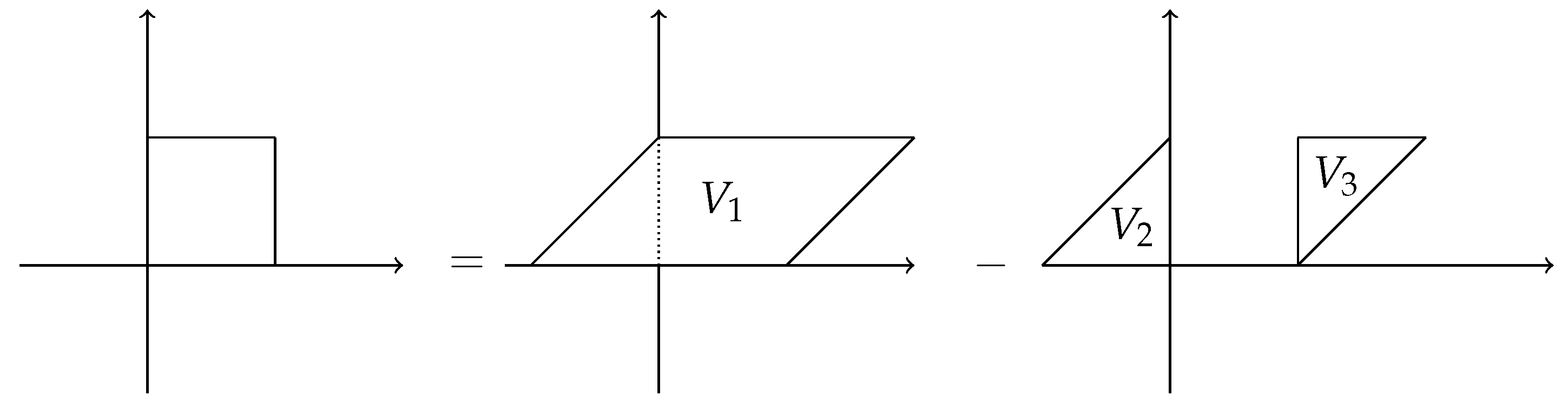
To calculate ${\tilde{A}}_{n,m}$, through imitating the method in [5], $[0,1]\times [0,1]$ can be represented by a parallelogram $V_1$ minus two triangles $V_2$ and $V_3$ (see Figure 2), where $V_1$ is enclosed by the lines $y=0$, $y=1$, $y-x=1$ and $y-x=-1$; $V_2$ is enclosed by $x=0$, $y=0$ and $y-x=1$; and $V_3$ is enclosed by $x=1$, $y=1$ and $y-x=-1$.

Figure 2. Domains for calculating ${\tilde{A}}_{n,m}$.

By denoting

$$\begin{array}{cc}\hfill {\tilde{R}}_{n,m}^1& ={\int \int }_{V_1}{|x-y|}^{2H-2}sin\left(n^{\ast }x\right)sin\left(m^{\ast }y\right)\mathrm{d}x\mathrm{d}y\hfill \end{array}$$

(87)

$$\begin{array}{cc}\hfill {\tilde{R}}_{n,m}^{2,3}& ={\int \int }_{V_2\cup V_3}{|x-y|}^{2H-2}sin\left(n^{\ast }x\right)sin\left(m^{\ast }y\right)\mathrm{d}x\mathrm{d}y,\hfill \end{array}$$

(88)

it’s clear that

$${\tilde{A}}_{n,m}=H(2H-1)({\tilde{R}}_{n,m}^1-{\tilde{R}}_{n,m}^{2,3}).$$

(89)

By changing the variables $u=y-x$, $v=y$ in double integral, the following can be deduced:

$${\tilde{R}}_{nm}^1={\int }_0^{1}sin\left(m^{\ast }v\right)sin\left(n^{\ast }v\right)\mathrm{d}v{\int }_{-1}^1{\left|u\right|}^{2H-2}cos\left(n^{\ast }u\right)\mathrm{d}u.$$

(90)

To calculate ${\tilde{R}}_{n,m}^{2,3}$, first of all, perform the mapping $V_3$ to $V_2$ by changing variables $x^{\prime }=1-x$, and $y^{\prime }=1-y$. Then, the integral over this region is greatly simplified under the change of variables $u=x+y$, $v=x-y$, which gives the following:

$${\tilde{R}}_{n,m}^{2,3}=\frac{{(-1)}^{m+n+1}}{2}{\int }_0^1{u}^{2H-2}\mathrm{d}u{\int }_{-u}^{u}cos(n^{\ast }\frac{u-v}{2}+{(-1)}^{m+n}{m}^{\ast }\frac{v+u}{2})\mathrm{d}v.$$

To calculate ${\tilde{A}}_{n,m}^{\left(1\right)}$, two sub-domains $I_1$, $I_2$ are chosen as is done in Step 3.1. of Section 5.1. Designating

$$\begin{array}{c}\hfill {\tilde{Q}}_{n,m}^1={\int \int }_{I_1}{(x+y)}^{2H-2}sin\left(n^{\ast }x\right)sin\left(m^{\ast }y\right)\mathrm{d}x\mathrm{d}y\end{array}$$

(91)

$$\begin{array}{c}\hfill {\tilde{Q}}_{n,m}^2={\int \int }_{I_2}{(x+y)}^{2H-2}sin\left(n^{\ast }x\right)sin\left(m^{\ast }y\right)\mathrm{d}x\mathrm{d}y\end{array}$$

(92)

it gives the following:

$${\tilde{A}}_{n,m}^{\left(1\right)}=2H(2H-1)({\tilde{Q}}_{n,m}^1+{\tilde{Q}}_{n,m}^2).$$

(93)

Step 2. Now, it is time to extract diagonal and off-diagonal information from ${\left({\tilde{A}}_{sub}\right)}_{n,m}$. By setting ${\left({\tilde{D}}_{sub}\right)}_{n,m}={\left({\tilde{A}}_{sub}\right)}_{n,m}{\delta }_{n,m}$, and ${\left({\tilde{O}}_{sub}\right)}_{n,m}={\left({\tilde{A}}_{sub}\right)}_{n,m}-{\tilde{D}}_{n,m}$, a decomposition ${\left({\tilde{A}}_{sub}\right)}_{n,m}={\left({\tilde{D}}_{sub}\right)}_{n,m}+{\left({\tilde{O}}_{sub}\right)}_{n,m}$ is obtained. Moreover, there hold the following:

$$\begin{array}{cc}\hfill {\left({\tilde{D}}_{sub}\right)}_{n,n}=& 2H(2H-1)({\tilde{R}}_{n,n}^1-{\tilde{R}}_{n,n}^{2,3}-{\tilde{Q}}_{n,n}^1-{\tilde{Q}}_{n,n}^2),\hfill \end{array}$$

(94)

$$\begin{array}{cc}\hfill {\left({\tilde{O}}_{sub}\right)}_{n,m}=& 2H(2H-1)({\tilde{R}}_{n,m}^1-{\tilde{R}}_{n,m}^{2,3}-{\tilde{Q}}_{n,m}^1-{\tilde{Q}}_{n,m}^2),n\ne m.\hfill \end{array}$$

(95)

The details for handling the ${\tilde{A}}_{n,m}$ part are emphasized, but the ones for ${\tilde{A}}_{n,m}^{\left(1\right)}$ are omitted, except for the conclusions.

Step 2.1. Calculate ${\tilde{A}}_{n,m}$ and ${\tilde{A}}_{n,m}^{\left(1\right)}$ in the case of $m>n\gg 1$. Simple calculations show the following:

$$\begin{array}{cc}\hfill {\tilde{R}}_{n,m}^1& =0.\hfill \end{array}$$

(96)

$$\begin{array}{cc}\hfill {\tilde{R}}_{n,m}^{2,3}& =\frac{{(-1)}^{m+n+1}}{m^{\ast }+{(-1)}^{m+n}{n}^{\ast }}{\int }_0^1{u}^{2H-2}(sin\left(m^{\ast }u\right)+{(-1)}^{m+n}sin\left(n^{\ast }u\right))\mathrm{d}u.\hfill \end{array}$$

(97)

Processing, as in Step 3 in Section 5.1, it is no trouble to verify the following:

$$\begin{array}{cc}\hfill & \begin{array}{cc}\hfill {\tilde{Q}}_{n,m}^1=& -\frac{1}{2(m^{\ast }+n^{\ast })}{\int }_0^1{u}^{2H-2}(sin\left(m^{\ast }u\right)+sin\left(n^{\ast }u\right))\mathrm{d}u\hfill \\ \hfill & +\frac{1}{2(m^{\ast }-n^{\ast })}{\int }_0^1{u}^{2H-2}(sin\left(m^{\ast }u\right)-sin\left(n^{\ast }u\right))\mathrm{d}u.\hfill \end{array}\hfill \end{array}$$

(98)

$$\begin{array}{cc}\hfill & \begin{array}{cc}\hfill {\tilde{Q}}_{n,m}^2=& \frac{{(-1)}^{m+n}}{2(m^{\ast }+n^{\ast })}{\int }_1^2{u}^{2H-2}(sin\left(m^{\ast }u\right)+sin\left(n^{\ast }u\right))\mathrm{d}u\hfill \\ \hfill & +\frac{{(-1)}^{m-n}}{2(m^{\ast }-n^{\ast })}{\int }_1^2{u}^{2H-2}(sin\left(m^{\ast }u\right)-sin\left(n^{\ast }u\right))\mathrm{d}u.\hfill \end{array}\hfill \end{array}$$

(99)

Using (51), (53), (55) and (58), it implies the following:

$$\begin{array}{cc}\hfill & {\tilde{R}}_{n,m}^1-{\tilde{R}}_{n,m}^{2,3}-{\tilde{Q}}_{n,m}^1-{\tilde{Q}}_{n,m}^2\hfill \\ \hfill =& \frac{3{(-1)}^{m+n}\Gamma (2H-1)cos\left(\pi H\right)}{2(m^{\ast }+{(-1)}^{m+n}{n}^{\ast })}(\frac{1}{m^{\ast 2H-1}}+{(-1)}^{m+n}\frac{1}{n^{\ast 2H-1}})\hfill \\ \hfill & +{(-1)}^{m+n}\frac{\Gamma (2H-1)cos\left(\pi H\right)}{2(m^{\ast }-{(-1)}^{m+n}{n}^{\ast })}(\frac{1}{m^{\ast 2H-1}}-{(-1)}^{m+n}\frac{1}{n^{\ast 2H-1}})+O\left(\frac{1}{mn}\right).\hfill \end{array}$$

(100)

Using the same techniques as Step 3.3 with Lemma 3, it is obvious that ${\tilde{R}}_{n,m}^1-{\tilde{R}}_{n,m}^{2,3}-{\tilde{Q}}_{n,m}^1-{\tilde{Q}}_{n,m}^2\asymp m^{-1}{n}^{2H-1}.$

Step 2.2. Calculate ${\tilde{A}}_{n,m}$ and ${\tilde{A}}_{n,m}^{\left(1\right)}$ in the case of $m=n\gg 1$. It is easy to check the following:

$$\begin{array}{cc}\hfill & \begin{array}{cc}\hfill {\tilde{R}}_{m,m}^1=& {\int }_0^{1}sin\left(m^{\ast }v\right)sin\left(m^{\ast }v\right)\mathrm{d}v{\int }_{-1}^1{\left|u\right|}^{2H-2}cos\left(m^{\ast }u\right)\mathrm{d}u\hfill \\ \hfill =& 2(\frac{\Gamma (2H-1)sin\left(\pi H\right)}{m^{\ast 2H-1}}+\frac{{(-1)}^m}{m^{\ast }}+O\left(\frac{1}{m^2}\right))\hfill \end{array}\hfill \end{array}$$

(101)

$$\begin{array}{cc}\hfill & \begin{array}{cc}\hfill {\tilde{R}}_{m,m}^{2,3}=& -\frac{1}{m^{\ast }}{\int }_0^1{u}^{2H-2}sin\left(m^{\ast }u\right)\mathrm{d}u\hfill \\ \hfill =& \frac{\Gamma (2H-1)cos\left(\pi H\right)}{m^{\ast 2H}}+O\left(\frac{1}{m^3}\right).\hfill \end{array}\hfill \end{array}$$

(102)

Following the similar procedures as Step 3. in Section 5.1, there holds the following:

$$\begin{array}{cc}\hfill {\tilde{Q}}_{m,m}^1=& \frac{1}{2}{\int }_0^1{u}^{2H-1}cos\left(m^{\ast }u\right)\mathrm{d}u-\frac{1}{2m^{\ast }}{\int }_0^1{u}^{2H-2}sin\left(m^{\ast }u\right)\mathrm{d}u.\hfill \end{array}$$

(103)

$$\begin{array}{cc}\hfill {\tilde{Q}}_{m,m}^2=& \frac{1}{2m^{\ast }}{\int }_1^2{u}^{2H-2}sin\left(m^{\ast }u\right)\mathrm{d}u+\frac{1}{2}{\int }_1^2{u}^{2H-1}cos\left(m^{\ast }u\right)\mathrm{d}u-{\int }_1^2{u}^{2H-2}cos\left(m^{\ast }u\right)\mathrm{d}u.\hfill \end{array}$$

(104)

Using (50)–(52) and (57), it leads to the following:

$$\begin{array}{cc}& {\tilde{R}}_{n,n}^1-{\tilde{R}}_{n,n}^{2,3}-{\tilde{Q}}_{n,n}^1-{\tilde{Q}}_{n,n}^2\hfill \\ \hfill =& \frac{2\Gamma (2H-1)sin\left(\pi H\right)}{n^{\ast 2H-1}}-\frac{(2\Gamma (2H)+3\Gamma (2H-1\left)\right)cos\left(\pi H\right)}{2n^{\ast 2H}}+O\left(\frac{1}{n^2}\right).\hfill \end{array}$$

Step 2.3. Summarize the asymptotic information for the matrix elements of ${\tilde{A}}_{sub}$. The asymptotics for the diagonal piece of ${\left({\tilde{A}}_{sub}\right)}_{n,m}$ are as follows:

$${\left({\tilde{D}}_{sub}\right)}_{m,m}=\frac{2\Gamma (2H+1)sin\left(\pi H\right)}{m^{\ast 2H-1}}-\frac{(4H+1)\Gamma (2H+1)cos\left(\pi H\right)}{2m^{\ast 2H}}+O\left(\frac{1}{m^2}\right)$$

(105)

if $m\gg 1$, and the ones for the off-diagonal piece are as follows:

$${\left({\tilde{O}}_{sub}\right)}_{n,m}\asymp \frac{1}{m{n}^{2H-1}}$$

(106)

if $m>n\gg 1$.

Step 3. Noticing that ${\tilde{D}}_{sub}$ is self-adjoint and positive, given any $\beta \in (0,1)$, ${\tilde{O}}_{sub}$ can also be written as ${\tilde{O}}_{sub}={\tilde{D}}_{sub}^{\beta }{\widehat{O}}_{der}{\tilde{D}}_{sub}^{\beta }$ with ${\widehat{O}}_{der}={\tilde{D}}_{sub}^{-\beta }{\tilde{O}}_{sub}{\tilde{D}}_{sub}^{-\beta }$. Since the order of the elements of ${\tilde{D}}_{sub}^{-\beta }$ is $m^{\beta (2H-1)}$ when $m\gg 1$, the order of the ones of ${\widehat{O}}_{der}$ is $m^{(2H-1)\beta -1}{n}^{(2H-1)\beta -2H+1}$ when $m>n\gg 1$. If $\beta \in (0,\frac{1}{2})$, it is easy to verify whether the elements of ${\widehat{O}}_{der}$ are square summable. In fact,

$$\begin{array}{cc}\hfill \sum _{m>n}{\left({\widehat{O}}_{der}\right)}_{n,m}^2\lesssim & \sum _{m>n}{m}^{2(2H-1)\beta -2}{n}^{2(2H-1)\beta -4H+2}\hfill \\ \hfill =& \sum _n{n}^{2(2H-1)\beta -4H+2}\sum _{m=n+1}^{\infty }{m}^{2(2H-1)\beta -2}\hfill \\ \hfill \lesssim & \sum _n{n}^{4(2H-1)\beta -4H+1}.\hfill \end{array}$$

The square summability of ${\widehat{O}}_{der}$ is verified since $4(2H-1)\beta -4H+1\in (-4H+1,-1)$ when $\beta \in (0,\frac{1}{2})$. Therefore, ${\widehat{O}}_{der}$ is a Hilbert–Schmidt operator (and thus compact). Using Lemma 4, it is immediately obtained the following:

$$|{\lambda }_n\left({\tilde{O}}_{sub}\right)|\lesssim n^{-2H+\frac{1}{2}+\delta }.$$

(107)

Setting $K_1={\tilde{D}}_{sub}$, $K_2={\tilde{O}}_{sub}$ and $j=n^{\alpha }$ in Lemma 5, it can be deduced the following:

$${\lambda }_n\left({\tilde{A}}_{sub}\right)\le \frac{{\kappa }_H}{n^{2H-1}}+O\left(n^{-2H+\alpha }\right)+O\left(n^{-\alpha (2H-\frac{1}{2}-\delta )}\right).$$

(108)

Choosing $2H-\alpha =\alpha (2H-\frac{1}{2})$(i.e., $\alpha =\frac{2H}{2H+\frac{1}{2}}$), it implies the following:

$${\lambda }_n\left({\tilde{A}}_{sub}\right)\le \frac{{\kappa }_H}{n^{2H-1}}+o\left(n^{-\frac{2H(4H-1)}{4H+1}+\delta }\right).$$

(109)

Repeating the argument with $K_1={\tilde{A}}_{sub}$, $K_2=-{\tilde{O}}_{sub}$ gives the following:

$${\lambda }_n\left({\tilde{A}}_{sub}\right)\ge \frac{{\kappa }_H}{n^{2H-1}}+o\left(n^{-\frac{2H(4H-1)}{4H+1}+\delta }\right).$$

(110)

The proof is completed.□

6. Discussion

Asymptotics for the Karhunen–Loève eigenvalues for a sub-fractional Brownian motion are proved, based on functional analysis method. However, those asymptotics are too rough to be simulated since the magnitude of data storage for the discretization of the corresponding eigenproblem is so huge, even for the small precision. The authors believe that it is limited by the current method to obtain those asympotics. It was expected that more accurate asympotics would be established if the idea in [6] could be applicable in this case. In principle, a circumvention of loss of translation structure in this eigenproblem should exist. To find an effective asymptotics method of analysis for the eigenproblem is our next goal.

7. Comments

At first, the authors were inspired by the idea in [6] and tried to use that method to solve the eigenproblem for sub-fractional Brownian motion. However, the algebraic structure of the Laplace transform of the eigenequation turned out to be different. Hence, the authors thought that the method in [6] was possibly unapplicable in the case of sub-fractional Brownian motion. In [12], the covariance of Brownian motion is considered a “perturbation” of the one of fractional Brownian motion. It inspired the authors to consider the term ${(s+t)}^{2H}$ in the covariance function to be a “perturbation” of the covariance of fractional Brownian motion. It still did not work after the elementary trial. This could also be an important part of our further research.