FPAA-Based Realization of Filters with Fractional Laplace Operators of Different Orders

Abstract

A simple and direct procedure for implementing fractional-order filters with transfer functions that contain Laplace operators of different fractional orders is presented in this work. Based on a general fractional-order transfer function that describes fractional-order low-pass, high-pass, band-pass, band-stop and all-pass filters, the introduced concept deals with the consideration of this function as a whole, with its approximation being performed using a curve-fitting-based technique. Compared to the conventional procedure, where each fractional-order Laplace operator of the transfer function is individually approximated, the main offered benefit is the significant reduction in the order of the resulting rational function. Experimental results, obtained using a field-programmable analog array device, verify the validity of this concept.

1. Introduction

Fractional-order filters have thrust the scientific field of filtering into a new era, making it applicable in a wide range of interdisciplinary fields, such as control systems, bio-impedance spectroscopy, acoustic applications and filter applications [1]. The insertion of one or more fractional exponents in a filter function provides additional degrees of freedom that allow precise adjustment of the filter’s characteristics, including the cutoff frequency and the slope of the transition from the pass band to stop band.

A general transfer function, able to describe fractional-order low-pass (LP), high-pass (HP), band-pass (BP), band-stop (BS) and all-pass (AP) filters, is given in (1)

$$H\left(s\right) = \frac{K_{HP}{\left(\tau s\right)}^{\alpha +\beta }+K_{BP}{\left(\tau s\right)}^{\beta }+K_{LP}}{{\left(\tau s\right)}^{\alpha +\beta }+{\left(\tau s\right)}^{\beta }+1},$$

(1)

where $\alpha ,\beta \in \left(0,1\right)$ are fractional orders; s is the Laplace operator; $\tau$ is a characteristic time constant; and $K_{LP}$, $K_{HP}$ and $K_{BP}$ are real coefficients denoting the gain factors of the LP, HP and BP filters, respectively. The BS filter is obtained by the sum of the LP and HP filter functions, and the AP filter by the subtraction of the LP from the HP filter function [2].

The implementation of the filter functions, generated from (1), cannot be directly performed using conventional elements. Therefore, the following alternative methods are exploited:

(a)

Employment of fractional-order capacitors, which substitute the conventional (i.e., integer-order) capacitors in the topologies of integer-order standard filters. Due to the absence of commercial availability of such elements, they are approximated by RC schemes, such as the Foster and Cauer networks. The price paid for the offered quick design procedure is the absence of on-the-fly tuning of the filter’s characteristics, making it suitable only for cases of filters with pre-defined type and frequency characteristics [3,4,5].

(b)

Approximation of the fractional-order Laplace operators in (1) using appropriate tools, such as Continued Fraction Expansion, Oustaloup, Matsuda and Carlson [6], and then substitution of the resulting rational function approximations of these operators. The derived filter function is an integer-order polynomial ratio that can be implemented utilizing classical filter design techniques, such as cascade connection of elementary filter stages and multi-feedback structures. This design procedure is more complicated than the previous one, but it offers the advantage of electronic tuning capability of the derived filter structures, considering that active elements with electronically controlled characteristics (e.g., transconductance) are utilized [2,7,8,9,10,11]. However, this approach is efficient only for approximations of filter functions with a single fractional order. In the case of functions, such as the one in (1), the order of the derived rational function will be at least double the applied order of approximation [2].

The contribution made in this work is summarized as follows:

(a)

Instead of individually approximating the fractional-order Laplace operators, the magnitude and phase frequency responses of the whole filter function in (1) are fitted by a suitable integer-order transfer function derived through the employment of specialized Symbolic Math Toolbox™ built-in functions.

(b)

The order of the derived rational function is always equal to the order of the employed approximation, and thus, this approach offers the advantage of minimizing the circuit complexity, compared to the aforementioned conventional approach.

The paper is organized as follows: an investigation of the problem regarding the approximation of the general filter function following the conventional and the proposed procedures is discussed in Section 2, and a design example for comparison purposes is given in Section 3. The validity of the suggested procedure was experimentally evaluated using a field-programmable analog array (FPAA) device [12] and the results are presented in Section 4.

2. Proposed Design Procedure

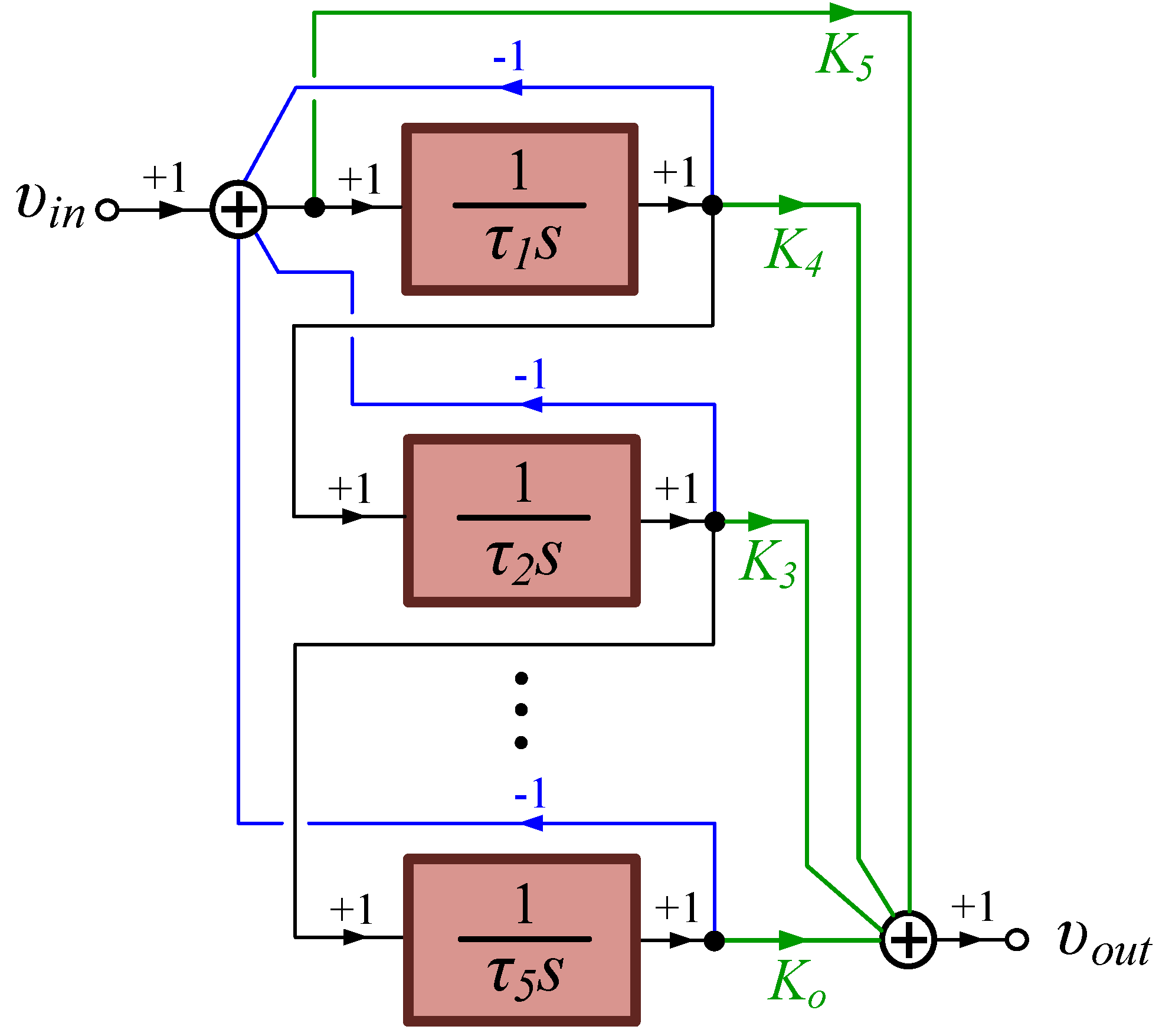
Using any of the continued fraction expansion, Oustaloup, Matsuda or Carlson methods, for the approximation of the Laplace operators in (1), the transfer function in (2) is derived this way:

$${\left(\tau s\right)}^r\simeq \frac{A_n{s}^n+A_{n-1}{s}^{n-1}+\dots +A_{1}s+A_0}{s^n+B_{n-1}{s}^{n-1}+\dots +B_{1}s+B_0},$$

(2)

where $r = \{\beta ,\alpha +\beta \}$ is the order of the operator; n is the order of the applied approximation; and $A_i$$(i = 0,1,\dots n)$, $B_j$$(j = 0,1,\dots n-1)$ are real, positive coefficients.

By approximating each one of the fractional terms ${\left(\tau s\right)}^{\beta }$ and ${\left(\tau s\right)}^{\alpha +\beta }$ of (1) using (2), the resulting approximated filter function will have the form of a rational, integer-order polynomial ratio, is that given in (3):

$$H_{approx}\left(s\right)\simeq \frac{C_p{s}^p+C_{p-1}{s}^{p-1}+\dots +C_{1}s+C_0}{s^q+D_{q-1}{s}^{q-1}+\dots +D_{1}s+D_0},$$

(3)

where $\left[p,q\right]$ is the order of the ratio’s polynomials and $C_k$, $(k = 0,1,\dots p)$, $D_l$, $(l = 0,1,\dots q-1)$ are real coefficients.

In the case that $\alpha +\beta \in \left(0,1\right)$, the nth-order approximation of the fractional terms ${\left(\tau s\right)}^{\beta }$ and ${\left(\tau s\right)}^{\alpha +\beta }$ is performed by transfer functions of the form of (2) with order equal to n. Therefore, the transfer function in (3) will be of order $2n$, due to the different values of the coefficients of the corresponding intermediate transfer functions used for approximating the Laplace operators. In the case that $\alpha +\beta \in \left(1,2\right)$, the approximation of the term ${\left(\tau s\right)}^{\alpha +\beta }$ is performed through the utilization of the product ${\left(\tau s\right)}^{(\alpha +\beta )-1}·\left(\tau s\right)$, and the resulting orders of the transfer function in (3) are summarized in

Table 1. Order of the functions in (3) for different types of filters using conventional approximation methods.

Filter	Order
	$\mathit{\alpha }\mathbf{+}\mathit{\beta }\mathbf{\in }\left(\mathbf{0}\mathbf{,}\mathbf{1}\right)$	$\mathit{\alpha }\mathbf{+}\mathit{\beta }\mathbf{\in }\left(\mathbf{1}\mathbf{,}\mathbf{2}\right)$
LP	$\left[p,q\right] = \left[2n,2n\right]$	$\left[p,q\right] = \left[2n,2n+1\right]$
HP		$\left[p,q\right] = \left[2n+1,2n+1\right]$
BP		$\left[p,q\right] = \left[2n,2n+1\right]$
BS		$\left[p,q\right] = \left[2n+1,2n+1\right]$
AP		$\left[p,q\right] = \left[2n+1,2n+1\right]$

.

The main derivation is that, for a given order of approximation $\left(n\right)$, the order of the final filter function will be at least the double, which means increased circuit complexity. The proposed concept suggests the exploitation of a curve-fitting-based approximation technique, which is based on the Sanathanan–Koerner (SK) least square iterative method, for approaching the filter function in (1) [8,9]. The application of this technique is simple, considering that it is supported by MATLAB software and specialized Symbolic Math Toolbox™ built-in functions. The main advantage of this method, compared to conventional approximation tools, is the capability of approaching a whole transfer function, leading to an expression that always has the simple form of (3). In addition, this method has already been compared with other relevant frequency response-based approximation algorithms, and it has proven to be more efficient in terms of accuracy [8,13].

The steps of the algorithm are:

step #1:

Extraction of the frequency response data of (1) within a specific frequency range of interest, a process that is performed using the frd built-in function.

step #2:

Approximation of the obtained data, based on the fitfrd built-in function, which forms the state-space model of the data for a given order of approximation $\left(n\right)$.

step #3:

Conversion of the model to an integer-order transfer function of the form in (3) using the ss2tf built-in function.

Therefore, the final approximated filter function, for an nth-order approximation, will be of order $\left[n,n\right]$ independent of the type of the filter, and this is the most attractive benefit offered by the proposed procedure. As the transfer function in (3) will have a constant form, the selection of the type of filter, as well as the tuning of its characteristics, will be performed through the adjustment of the values of the coefficients $C_k$ and $D_l$. This results in a versatile structure whose behavior can be externally determined without any change in its core. In other words, following the proposed procedure, an electronically adjustable or programmable structure can be employed for simultaneously offering the elementary LP, HP, BP, BS and AP filter functions with minimized active component count, and therefore, reduced circuit complexity, compared to the structures presented in [2].

3. Design Example and Comparative Results

The initial function in (1) was approximated using the proposed procedure, based on the curve-fitting technique, for order $n = 5$ within the frequency range $f = \left[10,100k\right]$ Hz for the filter cases given in

Table 2. Values of parameters in (1) for realizing various filter cases.

Filter	Parameter
	$\left(\mathit{\alpha },\mathit{\beta }\right)$	$\left({\mathit{K}}_{\mathit{LP}},{\mathit{K}}_{\mathit{HP}},{\mathit{K}}_{\mathit{BP}}\right)$	$\mathit{\tau }$
LP	$\left(0.3,0.5\right)$	$\left(1,0,0\right)$	$22.91\left(\mathsf{\mu }\mathrm{s}\right)$
	$\left(0.3,0.8\right)$		$69.97\left(\mathsf{\mu }\mathrm{s}\right)$
HP	$\left(0.5,0.3\right)$	$\left(0,1,0\right)$	$1.106\left({m}\mathrm{s}\right)$
	$\left(0.8,0.3\right)$		$362\left(\mathsf{\mu }\mathrm{s}\right)$
BP	$\left(0.4,0.7\right)$	$\left(0,0,1\right)$	$186.7\left(\mathsf{\mu }\mathrm{s}\right)$
	$\left(0.7,0.4\right)$		$135.7\left(\mathsf{\mu }\mathrm{s}\right)$
BS	$\left(0.4,0.7\right)$	$\left(1,1,0\right)$	$205\left(\mathsf{\mu }\mathrm{s}\right)$
	$\left(0.7,0.4\right)$		$123.5\left(\mathsf{\mu }\mathrm{s}\right)$
AP	$\left(0.3,0.5\right)$	$\left(-1,1,0\right)$	$184.8\left(\mathsf{\mu }\mathrm{s}\right)$
	$\left(0.6,0.8\right)$		$547.8\left(\mathsf{\mu }\mathrm{s}\right)$

. In order to prove the efficiency of the proposed concept, a comparison with the Oustaloup approximation method of the same order $\left(n = 5\right)$ was also performed.

The final filter function, derived following the proposed approximation process, is that given in (3) with $\left[p,q\right] = \left[5,5\right]$ for all types of filters. This is not the case following the Oustaloup method, where, by consulting the Table 1, the order of the obtained function is $\left[p,q\right] = \left[10,11\right]$ for the LP and BP types, and $\left[p,q\right] = \left[11,11\right]$ for the HP, BS and AP types. Therefore, the Oustaloup method leads to double the hardware compared to that required for the curve-fitting-based method. In addition, the fact that the derived filter function in the case of the proposed procedure has a common form in all filter types makes it possible to implement different types of filters with variable order using the same controllable core.

The efficiency of each approximation method was evaluated through the gain and phase frequency responses of Figure 1, obtained using the MATLAB software, where the Oustaloup results are indicated by dashed-dotted lines and the curve-fitting-based results by solid lines. Considering the associated ideal responses, which are indicated by dashed lines, the difference between the accuracy of the two methods is evident. In particular, the maximum integral absolute error (IAE) on the gain for the LP, HP, BP, BS and AP filter types was about $1.94\times {10}^4$ dB·Hz and in the phase $1.01\times {10}^7$ °·Hz in the case of the Oustaloup method. The corresponding values, in the case of the proposed approximation procedure, were $4.22\times {10}^3$ dB·Hz and $1.43\times {10}^6$ °·Hz. Consequently, the proposed approximation process offers not only a considerably compact transfer function that can be implemented with the requirement of minimum circuitry, but also a sufficiently accurate approximation over the entire frequency range of interest.

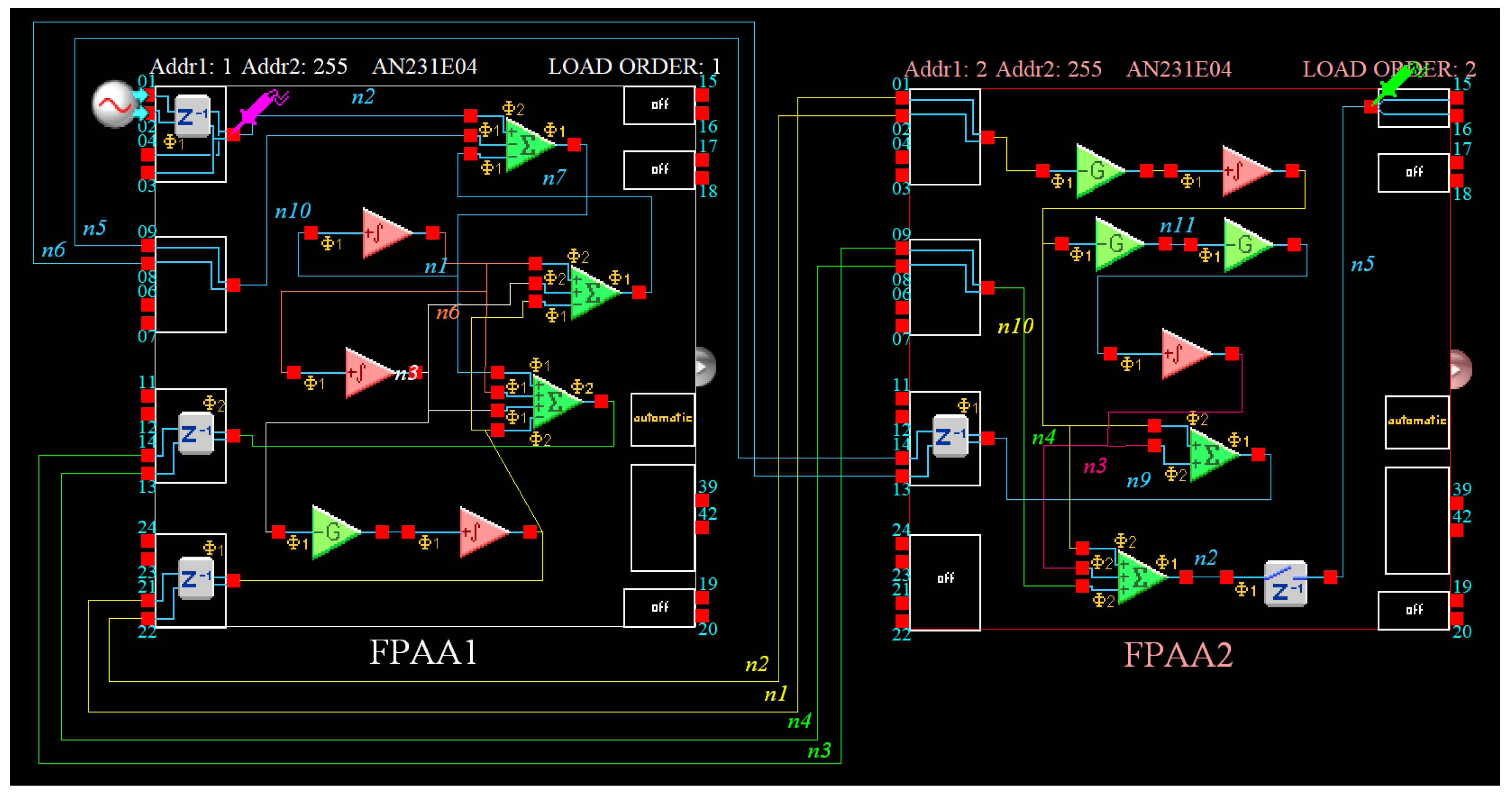
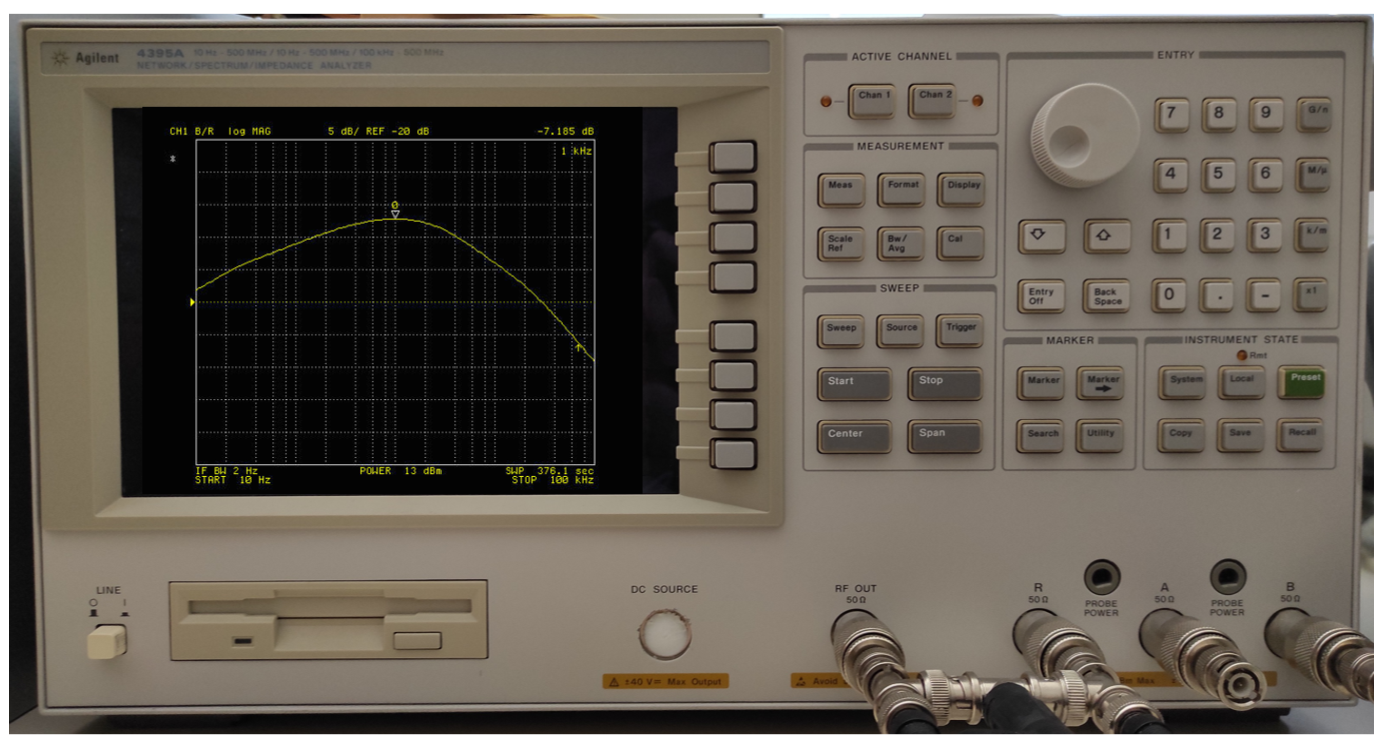
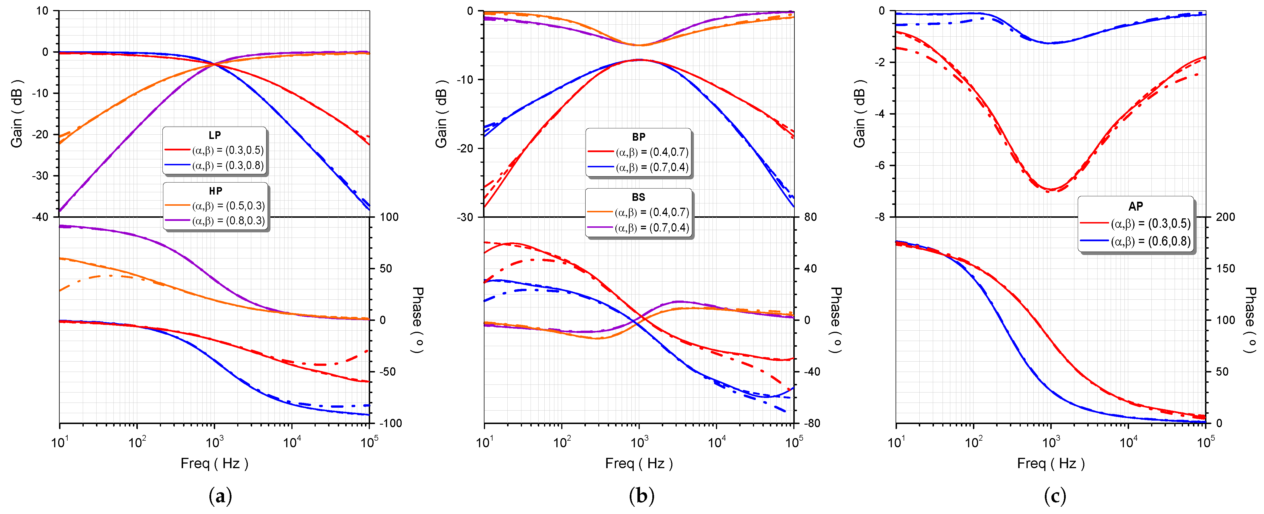
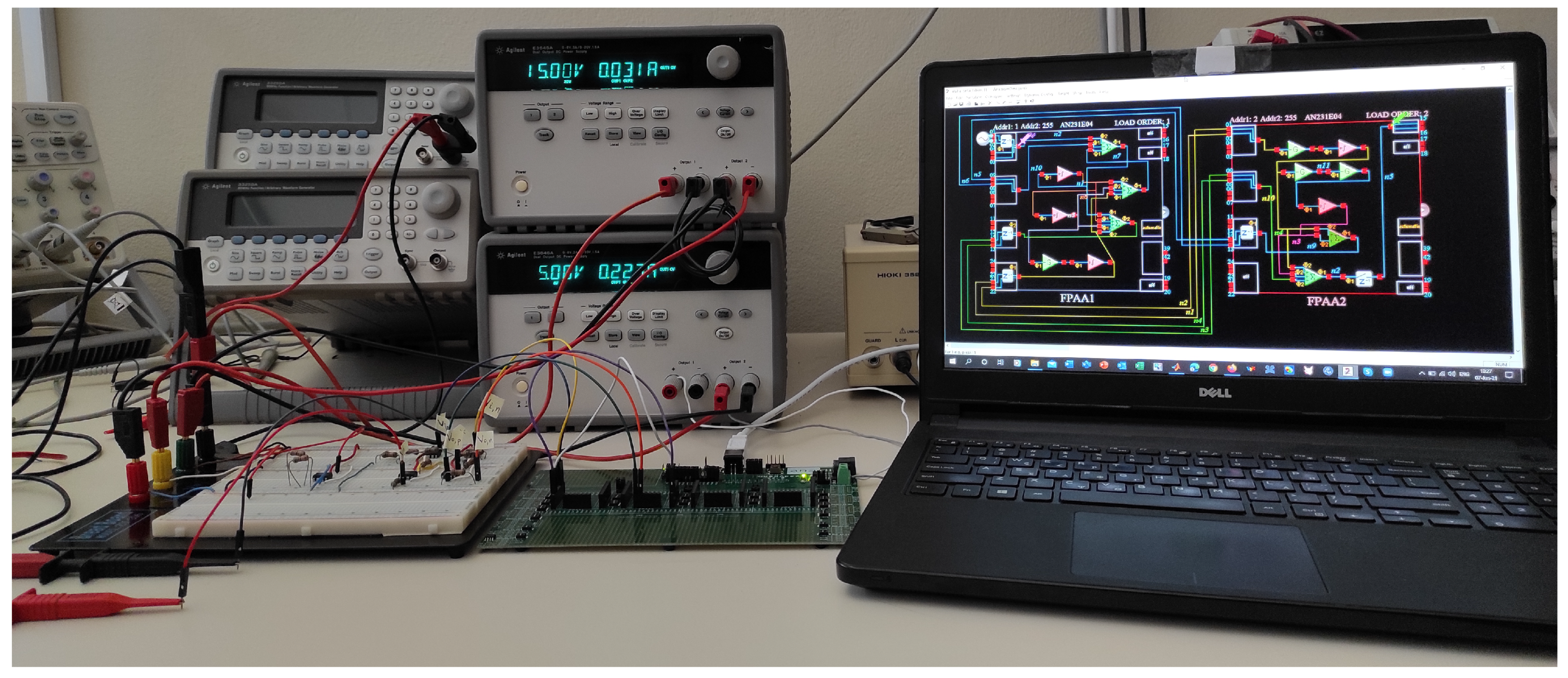
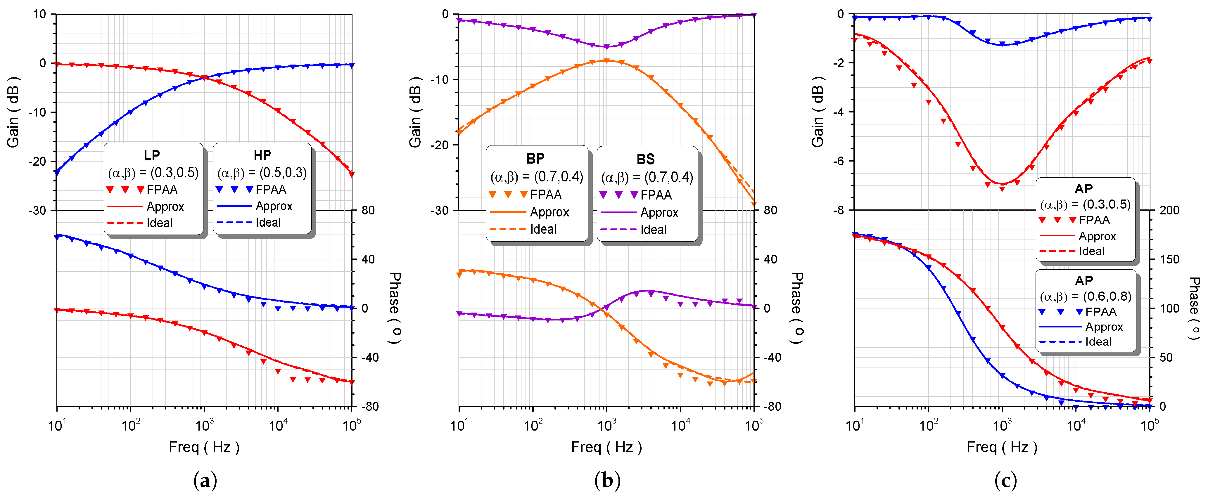
4. Experimental Results

The proposed concept was experimentally evaluated using FPAA hardware, and in particular, an Anadigm QUAD AN231K04 development kit, which is controlled through the AnadigmDesigner 2 EDA software [14,15,16,17,18]. Employing an integrator-based follow-the-leader feedback (FLF) structure, which is depicted in Figure 2, considering a 5th-order approximation, the transfer function that describes this functional block diagram is the following:

$$H_{FLF}\left(s\right) = \frac{K_5{s}^5+K_4{s}^4+\dots +K_{1}s+K_0}{s^5+\frac{1}{{\tau }_1}{s}^4+\dots +\frac{1}{{\tau }_1{\tau }_2\dots {\tau }_4}s+\frac{1}{{\tau }_1{\tau }_2\dots {\tau }_5}},$$

(4)

and the time constants ($\tau$) and scaling factors $\left(K\right)$ are calculated by equating the coefficients of (3) and (4). Therefore, the design equations, considering that $D_5 = 1$, becomes as follows:

$$K_i = {\displaystyle \frac{C_i}{D_i}},\left(i = 0,1,\dots 5\right){\tau }_{i+1} = {\displaystyle \frac{D_{5-i}}{D_{4-i}}},\left(i = 0,1,\dots 4\right).$$

(5)

For demonstration purposes, six of the cases, given in Table 2, were examined: (i) LP filter with $\left(\alpha ,\beta \right) = \left(0.3,0.5\right)$, (ii) HP filter with $\left(\alpha ,\beta \right) = \left(0.5,0.3\right)$, (iii) BP filter with $\left(\alpha ,\beta \right) = \left(0.7,0.4\right)$, (iv) BS filter with $\left(\alpha ,\beta \right) = \left(0.7,0.4\right)$, (v) AP filter with $\left(\alpha ,\beta \right) = \left(0.3,0.5\right)$ and (vi) AP filter with $\left(\alpha ,\beta \right) = \left(0.6,0.8\right)$. The coefficients of the derived approximated filter functions are provided in

Table 3. Values of the coefficients in (3) derived from the 5th-order approximation of the initial function in (1) for various filter types.

Coefficient	Filter
	LP	HP	BP	BS	AP
	$\left(\mathbf{0}.\mathbf{3},\mathbf{0}.\mathbf{5}\right)$	$\left(\mathbf{0}.\mathbf{5},\mathbf{0}.\mathbf{3}\right)$	$\left(\mathbf{0}.\mathbf{7},\mathbf{0}.\mathbf{4}\right)$	$\left(\mathbf{0}.\mathbf{7},\mathbf{0}.\mathbf{4}\right)$	$\left(\mathbf{0}.\mathbf{3},\mathbf{0}.\mathbf{5}\right)$	$\left(\mathbf{0}.\mathbf{6},\mathbf{0}.\mathbf{8}\right)$
${\mathit{C}}_{\mathbf{0}}$	$1.812\times {10}^{20}$	$2.383\times {10}^{15}$	$4.68\times {10}^{16}$	$6.689\times {10}^{17}$	$-1.026\times {10}^{19}$	$-1.146\times {10}^{19}$
${\mathit{C}}_{\mathbf{1}}$	$4.361\times {10}^{17}$	$1.811\times {10}^{14}$	$1.101\times {10}^{15}$	$5.767\times {10}^{15}$	$-3.783\times {10}^{16}$	$-6.374\times {10}^{15}$
${\mathit{C}}_{\mathbf{2}}$	$1.317\times {10}^{14}$	$8.018\times {10}^{11}$	$2.705\times {10}^{12}$	$7.219\times {10}^{12}$	$-8.754\times {10}^{12}$	$2.488\times {10}^{12}$
${\mathit{C}}_{\mathbf{3}}$	$6.778\times {10}^9$	$5.37\times {10}^8$	$1.139\times {10}^9$	$1.886\times {10}^9$	$2.109\times {10}^9$	$2.18\times {10}^9$
${\mathit{C}}_{\mathbf{4}}$	$5.138\times {10}^4$	$6.26\times {10}^4$	$2.169\times {10}^4$	$1.237\times {10}^5$	$1.555\times {10}^5$	$1.386\times {10}^5$
${\mathit{C}}_{\mathbf{5}}$	$0.02145$	$0.9617$	$0.01929$	$0.9802$	$0.8324$	$0.9842$
${\mathit{D}}_{\mathbf{0}}$	$1.871\times {10}^{20}$	$1.296\times {10}^{17}$	$5.653\times {10}^{17}$	$7.264\times {10}^{17}$	$1.11\times {10}^{19}$	$1.165\times {10}^{19}$
${\mathit{D}}_{\mathbf{1}}$	$5.069\times {10}^{17}$	$1.296\times {10}^{15}$	$5.51\times {10}^{15}$	$7.152\times {10}^{15}$	$5.894\times {10}^{16}$	$1.961\times {10}^{16}$
${\mathit{D}}_{\mathbf{2}}$	$1.966\times {10}^{14}$	$2.196\times {10}^{12}$	$8.418\times {10}^{12}$	$1.059\times {10}^{13}$	$4.652\times {10}^{13}$	$1.243\times {10}^{13}$
${\mathit{D}}_{\mathbf{3}}$	$1.65\times {10}^{10}$	$8.576\times {10}^8$	$2.753\times {10}^9$	$3.223\times {10}^9$	$7.759\times {10}^9$	$3.067\times {10}^9$
${\mathit{D}}_{\mathbf{4}}$	$3.144\times {10}^5$	$7.504\times {10}^4$	$1.368\times {10}^5$	$1.473\times {10}^5$	$2.532\times {10}^5$	$1.528\times {10}^5$

.

Using the values of Table 3 and the design equations in (5), the calculated values of time constants and scaling factors are summarized in

Table 4. Values of time constants and scaling factors in (4), calculated using the values of Table 3 and the design equations in (5).

Coefficient	Filter
	LP	P	BP	BS	AP
	$\left(\mathbf{0}.\mathbf{3},\mathbf{0}.\mathbf{5}\right)$	$\left(\mathbf{0}.\mathbf{5},\mathbf{0}.\mathbf{3}\right)$	$\left(\mathbf{0}.\mathbf{7},\mathbf{0}.\mathbf{4}\right)$	$\left(\mathbf{0}.\mathbf{7},\mathbf{0}.\mathbf{4}\right)$	$\left(\mathbf{0}.\mathbf{3},\mathbf{0}.\mathbf{5}\right)$	$\left(\mathbf{0}.\mathbf{6},\mathbf{0}.\mathbf{8}\right)$
${\mathit{K}}_{\mathbf{0}}$	$0.969$	$0.018$	$0.083$	$0.921$	$-0.924$	$-0.984$
${\mathit{K}}_{\mathbf{1}}$	$0.86$	$0.14$	$0.2$	$0.806$	$-0.642$	$-0.325$
${\mathit{K}}_{\mathbf{2}}$	$0.67$	$0.365$	$0.321$	$0.682$	$-0.188$	$0.2$
${\mathit{K}}_{\mathbf{3}}$	$0.41$	$0.626$	$0.414$	$0.585$	$0.272$	$0.711$
${\mathit{K}}_{\mathbf{4}}$	$0.163$	$0.834$	$0.158$	$0.84$	$0.614$	$0.907$
${\mathit{K}}_{\mathbf{5}}$	$0.021$	$0.962$	$0.019$	$0.98$	$0.832$	$0.984$
${\mathit{\tau }}_{\mathbf{1}}$	3.18 ($\mathsf{\mu }$s)	13.32 ($\mathsf{\mu }$s)	7.31 ($\mathsf{\mu }$s)	6.79 ($\mathsf{\mu }$s)	3.95 ($\mathsf{\mu }$s)	6.546 ($\mathsf{\mu }$s)
${\mathit{\tau }}_{\mathbf{2}}$	19.05 ($\mathsf{\mu }$s)	87.5  ($\mathsf{\mu }$s)	49.7 ($\mathsf{\mu }$s)	45.71 ($\mathsf{\mu }$s)	32.63 ($\mathsf{\mu }$s)	49.81 ($\mathsf{\mu }$s)
${\mathit{\tau }}_{\mathbf{3}}$	83.92 ($\mathsf{\mu }$s)	390.5 ($\mathsf{\mu }$s)	327 ($\mathsf{\mu }$s)	304.2 ($\mathsf{\mu }$s)	166.8 ($\mathsf{\mu }$s)	246.6 ($\mathsf{\mu }$s)
${\mathit{\tau }}_{\mathbf{4}}$	387.9 ($\mathsf{\mu }$s)	1.69 (ms)	1.53 (ms)	1.78 (ms)	789.25 ($\mathsf{\mu }$s)	634.1 ($\mathsf{\mu }$s)
${\mathit{\tau }}_{\mathbf{5}}$	2.71 (ms)	10 (ms)	9.75 (ms)	9.85 (ms)	5.31 (ms)	1.68 (ms)

.

The implementation of the FLF structure in Figure 2, using the FPAA hardware, was based on the configuration that is demonstrated in the Anadigm design of Figure 3. Two FPAA chips were required when Integrator, GainHold and SumDiff Configurable Analogue Blocks (CABs) were utilized to implement the integration and scaling stages, and the chip clock was set at $2$ MHz. The experimental setup that was used is shown in Figure 4.

The experimental gain and phase were measured using an Agilent 4395A spectrum analyzer within the frequency range $f = \left[10,100k\right]$ Hz, and the resulting responses are given in Figure 5a for the LP and HP filter types; in Figure 5b for the BP and BS types; and in Figure 5c for the AP filter type, indicated by triangle symbols, along with the respective results obtained from the curve-fitting-based approximation (solid lines) and the theory (dashed lines).

Indicatively, a screenshot of the analyzer, showing the gain frequency response during the measurement of the BP type of filter for orders $\left(\alpha ,\beta \right) = \left(0.7,0.4\right)$, is demonstrated in Figure 6. From these plots, the versatile features of the implemented FPAA-based structure were verified, making the presented procedure attractive from the design flexibility point of view.

The experimental values of the critical frequencies for each case are tabulated in

Table 5. Critical frequencies for the filter cases in Figure 5, along with the theoretical values given between parentheses.

Frequency	Filter
	LP	HP	BP	BS	AP
$f_c/f_{peak}$ (kHz)	1 (1)	1 (1)	1 (1)	1 (1)	1 (1)
$f_{low}$ (Hz)	–	–	142.5 (140.7)	173.8 (174.1)	–
$f_{high}$ (kHz)	–	–	4.36 (4.32)	3.48 (3.37)	–

, with the respective theoretically calculated values being given between parentheses, verifying the accurate behavior of the implemented filter functions.

5. Conclusions

The proposed concept for the implementation of fractional-order filter transfer functions with Laplace operators of multiple fractional orders, based on the exploitation of a curve-fitting-based approximation process, provides simultaneously an efficient and compact realization. The reduction in the order of the derived approximated rational transfer function was significant, compared to the case where conventional approximation methods were followed. The provided design example shows that, according to the presented procedure, the derived order of the transfer function for a 5th-order approximation was $\left[p,q\right] = \left[5,5\right]$ for all filter types with a maximum error of about $10\%$ in the frequency range $\left[10,100k\right]$ Hz. When employing the Oustaloup approximation, the order of the function was $\left[p,q\right] = \left[10,11\right]$ for the LP and BP types and $\left[11,11\right]$ for the HP, BS and AP types. The maximum observed error in the aforementioned frequency range was about $50\%$. Another resulting benefit is that all types of filters with variable orders can be implemented by the same core, making the presented structure a generalized filter scheme. This was experimentally verified through the utilization of the Anadigm QUAD AN231K04 development kit.

The employed algorithm offers the advantage of quick design procedure in the sense that the whole transfer function is considered, instead of the intermediate fractional-order Laplace terms. In addition, it approximates the fractional-order function within a frequency range defined by the user, as in the case of the Oustaloup method. The same also holds for similar MATLAB software Symbolic Math Toolbox™ built-in functions, such as tfest. On the other hand, a drawback is that these curve-fitting approximation methods are only available in MATLAB software. Another option could be employing the Padé tool, which performs approximation of the transfer function around a center frequency specified by the user, as in the case of the continued fraction expansion method. A comparison among all the aforementioned methods showed that the Sanathanan–Koerner (SK) least square iterative method employed in this work outperforms any of the other approximation tools [8,13].

The presented design procedure is versatile and can be also applied for the approximation of various types of fractional-order transfer functions, including control systems [19,20] and biological/biomedical systems [21], and these are undergoing research exploitation steps.

References

1. Tsirimokou, G.; Psychalinos, C.; Elwakil, A. Design of CMOS Analog Integrated Fractional-Order Circuits: Applications in Medicine and Biology; Springer: Berlin/Heidelberg, Germany, 2017. [Google Scholar]
2. Tsirimokou, G.; Psychalinos, C.; Elwakil, A.S. Fractional-order electronically controlled generalized filters. Int. J. Circuit Theory Appl. 2017, 45, 595–612. [Google Scholar] [CrossRef]
3. Sladok, O.; Koton, J.; Kubanek, D.; Dvorak, J.; Psychalinos, C. Pseudo-differential (2 + α)-order Butterworth frequency filter. IEEE Access 2021, 1. [Google Scholar] [CrossRef]
4. Biswal, K.; Tripathy, M.C.; Kar, S. Performance analysis of fractional order low-pass filter. In Advances in Intelligent Computing and Communication; Springer: Berlin/Heidelberg, Germany, 2020; pp. 224–231. [Google Scholar]
5. Mijat, N.; Jurisic, D.; Moschytz, G.S. Analog Modeling of Fractional-Order Elements: A Classical Circuit Theory Approach. IEEE Access 2021, 9, 110309–110331. [Google Scholar] [CrossRef]
6. Hamed, E.M.; AbdelAty, A.M.; Said, L.A.; Radwan, A.G. Effect of different approximation techniques on fractional-order KHN filter design. Circuits Syst. Signal Process. 2018, 37, 5222–5252. [Google Scholar] [CrossRef]
7. Langhammer, L.; Dvorak, J.; Sotner, R.; Jerabek, J.; Bertsias, P. Reconnection–less reconfigurable low–pass filtering topology suitable for higher–order fractional–order design. J. Adv. Res. 2020, 25, 257–274. [Google Scholar] [CrossRef] [PubMed]
8. Kapoulea, S.; Psychalinos, C.; Elwakil, A.S. Double exponent fractional-order filters: Approximation methods and realization. Circuits Syst. Signal Process. 2021, 40, 993–1004. [Google Scholar] [CrossRef]
9. Kapoulea, S.; Psychalinos, C.; Elwakil, A.S. Power law filters: A new class of fractional-order filters without a fractional-order Laplacian operator. AEU-Int. J. Electron. Commun. 2021, 129, 153537. [Google Scholar] [CrossRef]
10. Jerabek, J.; Sotner, R.; Dvorak, J.; Polak, J.; Kubanek, D.; Herencsar, N.; Koton, J. Reconfigurable fractional-order filter with electronically controllable slope of attenuation, pole frequency and type of approximation. J. Circuits Syst. Comput. 2017, 26, 1750157. [Google Scholar] [CrossRef] [Green Version]
11. Mahata, S.; Herencsar, N.; Kubanek, D. Optimal Approximation of Fractional-Order Butterworth Filter Based on Weighted Sum of Classical Butterworth Filters. IEEE Access 2021, 9, 81097–81114. [Google Scholar] [CrossRef]
12. Hasler, J.; Shah, S. An SoC FPAA based programmable, ladder-filter based, linear-phase analog filter. IEEE Trans. Circuits Syst. Regul. Pap. 2020, 68, 592–602. [Google Scholar] [CrossRef]
13. Xue, D. Fractional-Order Control Systems; de Gruyter: Berlin, Germany, 2017. [Google Scholar]
14. Anadigm. AN231E04 dpASP: The AN231E04 dpASP Dynamically Reconfigurable Analog Signal Processor. Available online: https://anadigm.com/an231e04.asp (accessed on 5 November 2021).
15. Freeborn, T.J.; Maundy, B.; Elwakil, A.S. Field programmable analogue array implementation of fractional step filters. IET Circuits Devices Syst. 2010, 4, 514–524. [Google Scholar] [CrossRef]
16. Freeborn, T.J.; Maundy, B. Incorporating FPAAs into laboratory exercises for analogue filter design. Int. J. Electr. Eng. Educ. 2013, 50, 188–200. [Google Scholar] [CrossRef]
17. Muñiz-Montero, C.; García-Jiménez, L.V.; Sánchez-Gaspariano, L.A.; Sánchez-López, C.; González-Díaz, V.R.; Tlelo-Cuautle, E. New alternatives for analog implementation of fractional-order integrators, differentiators and PID controllers based on integer-order integrators. Nonlinear Dyn. 2017, 90, 241–256. [Google Scholar] [CrossRef]
18. Tlelo-Cuautle, E.; Pano-Azucena, A.D.; Guillén-Fernández, O.; Silva-Juárez, A. Analog/Digital Implementation of Fractional Order Chaotic Circuits and Applications; Springer: Berlin/Heidelberg, Germany, 2020. [Google Scholar]
19. Lino, P.; Maione, G.; Stasi, S.; Padula, F.; Visioli, A. Synthesis of fractional-order PI controllers and fractional-order filters for industrial electrical drives. IEEE/CAA J. Autom. Sin. 2017, 4, 58–69. [Google Scholar] [CrossRef] [Green Version]
20. Azar, A.T.; Radwan, A.G.; Vaidyanathan, S. Fractional Order Systems: Optimization, Control, Circuit Realizations and Applications; Academic Press: Cambridge, MA, USA, 2018. [Google Scholar]
21. Mohsen, M.; Said, L.A.; Madian, A.H.; Radwan, A.G.; Elwakil, A.S. Fractional-Order Bio-Impedance Modeling for Interdisciplinary Applications: A Review. IEEE Access 2021, 9, 33158–33168. [Google Scholar] [CrossRef]
Figure 1. Gain and phase frequency responses, derived from 5th-order Oustaloup (dashed-dotted lines) and 5th-order curve-fitting-based (solid lines) approximation methods, for the (a) LP and HP, (b) BP and BS and (c) AP filter cases given in Table 2, along with the corresponding ideal responses (dashed lines).
Fractalfract 05 00218 g001
Figure 2. FLF block diagram for implementing LP, HP, BP, BS and AP filter functions.
Fractalfract 05 00218 g002
Figure 3. FPAA-based realization of the functional block diagram in Figure 2.
Fractalfract 05 00218 g003
Figure 4. Experimental setup for evaluating the performances of the filters.
Fractalfract 05 00218 g004
Figure 5. Experimental gain and phase frequency responses (triangle symbols), along with the corresponding approximated (solid lines) and ideal (dashed lines) responses, for (a) LP and HP, (b) BP and BS and (c) AP filter cases.
Fractalfract 05 00218 g005
Figure 6. Screenshot of the Agilent 4395A spectrum analyzer, showing the gain frequency response during the measurement of the BP type of filter for orders α , β   =   0.7 , 0.4 .
Fractalfract 05 00218 g006