A New Three-Step Root-Finding Numerical Method and Its Fractal Global Behavior

Abstract

There is an increasing demand for numerical methods to obtain accurate approximate solutions for nonlinear models based upon polynomials and transcendental equations under both single and multivariate variables. Keeping in mind the high demand within the scientific literature, we attempt to devise a new nonlinear three-step method with tenth-order convergence while using six functional evaluations (three functions and three first-order derivatives) per iteration. The method has an efficiency index of about 1.4678, which is higher than most optimal methods. Convergence analysis for single and systems of nonlinear equations is also carried out. The same is verified with the approximated computational order of convergence in the absence of an exact solution. To observe the global fractal behavior of the proposed method, different types of complex functions are considered under basins of attraction. When compared with various well-known methods, it is observed that the proposed method achieves prespecified tolerance in the minimum number of iterations while assuming different initial guesses. Nonlinear models include those employed in science and engineering, including chemical, electrical, biochemical, geometrical, and meteorological models.

1. Introduction

The study of iterative methods for solving nonlinear equations and systems appears to be a very important area in theory and practice. Such problems appear not only in applied mathematics but also in many branches of science including engineering (design of an electric circuit), physics (pipe friction), chemistry (greenhouse gases and rainwater), biology (steady-state of Lotka–Volterra system), fluid dynamics (combined conductive–radiative heat transfer), environmental engineering (oxygen level in a river downstream from a sewage discharge), finance (option pricing), and many more. The study of nonlinear models is a vital area of research in numerical analysis. Interesting applications in pure and applied sciences can be studied in the general construction of the nonlinear equations expressed in the form $g\left(x\right)=0$. Due to their significance, several iterative methods have been devised under certain situations since it is near to impossible to obtain exact solutions of models that are nonlinear in nature. These iterative methods have been constructed using different existing methods such as Taylor expansion, the perturbation method, the homotopy perturbation method, Adomian decomposition method, quadrature formula, multi-point iterative methods, the Steffensen-type methods adapted to multidimensional cases, and the variational iteration method. For detailed information, see [1,2,3,4,5,6,7,8]. Among existing iterative methods, the optimal methods are considered those that satisfy the condition for an order of convergence of $2^{k-1}$, where k stands for the number of function evaluations per iteration as suggested in [9]. In this way, Newton’s classical method $x_{n+1}=x_n-\frac{g\left(x_n\right)}{g^{\prime }\left(x_n\right)}$ is the optimal method with quadratic convergence. Various attempts have been made to improve the efficiency of Newton’s classical method in past and recent research, as can be seen in [10,11,12,13,14,15] and most of the references cited therein.

2. Materials and Methods

In a general form, the uni-variate nonlinear equation can be expressed as $g\left(x\right)=0$, where x is the desired quantity. It is extremely difficult to solve the nonlinear equation to find the value of x. Therefore, we attempt to devise a new, highly convergent iterative method to obtain an accurate approximate x that could yield the smallest possible error in the numerical solution. Before we continue with a discussion and derivation of the proposed method, we present some of the methods that are frequently used in the available literature. Later, we use these methods to compare the results obtained under these methods and the results obtained via the method we plan to propose.

2.1. Some Existing Methods

The iterative method, called the Newton Rahpson method $N{R}_2$ [1,16,17] with quadratic convergence, is shown below and uses two function evaluations: one for the function $g\left(x\right)$ itself and 1 for the first derivative $g^{\prime }\left(x\right)$:

$$x_{n+1}=x_n-{\displaystyle \frac{g\left(x_n\right)}{g^{\prime }\left(x_n\right)}},n=0,1,2,\dots ,$$

(1)

where $g^{\prime }\left(x_n\right)\ne 0.$

In [2], the authors proposed an iterative method with fifth-order convergence as abbreviated by $MH{M}_5$. The method requires four function evaluations per iteration: two for the function itself and two first derivatives. The computational steps for the two-step method $MH{M}_5$ is described below:

$$\begin{array}{cc}\hfill y_n& =x_n-{\displaystyle \frac{g\left(x_n\right)}{g^{\prime }\left(x_n\right)}},\hfill \\ \hfill x_{n+1}& =y_n-{\displaystyle \frac{g^{\prime }\left(y_n\right)+3g^{\prime }\left(x_n\right)}{5g^{\prime }\left(y_n\right)-g^{\prime }\left(x_n\right)}}.{\displaystyle \frac{g\left(y_n\right)}{g^{\prime }\left(x_n\right)}},\hfill \end{array}\begin{array}{c}n=0,1,2,\dots ,\hfill \end{array}$$

(2)

where $g^{\prime }\left(x_n\right)\ne 0$ and $5g^{\prime }\left(y_n\right)\ne g^{\prime }\left(x_n\right).$

An efficient three-step iterative method with sixth-order convergence is proposed in [3]. This method is the combination of two different methods from [1,18] with second and third-order convergence, respectively. The method requires five function evaluations: three evaluations of the function itself and two evaluations of the first-order derivative per iteration. We represent the method as $H{M}_6$. The computational steps of the method can be described as follows:

$$\begin{array}{cc}\hfill y_n& =x_n-{\displaystyle \frac{g\left(x_n\right)}{g^{\prime }\left(x_n\right)}},\hfill \\ \hfill z_n& =y_n-{\displaystyle \frac{g\left(y_n\right)}{g^{\prime }\left(y_n\right)}},\hfill \\ \hfill x_{x+1}& =y_n-{\displaystyle \frac{g\left(y_n\right)+g\left(z_n\right)}{g^{\prime }\left(y_n\right)}}.\hfill \end{array}\begin{array}{c}n=0,1,2,\dots ,\hfill \end{array}$$

(3)

The three-step method with eighth-order convergence as denoted by $W{O}_8$ is proposed in [19]. The method requires four function evaluations: three evaluations of the function itself and one evaluation of the first-order derivative per iteration. The computational steps of $W{O}_8$ can be described as follows:

$$\begin{array}{cc}\hfill y_n& =x_n-{\displaystyle \frac{g\left(x_n\right)}{g^{\prime }\left(x_n\right)}},\hfill \\ \hfill z_n& =x_n-{\displaystyle \frac{g\left(x_n\right)}{g^{\prime }\left(x_n\right)}}{\displaystyle \frac{4g{\left(x_n\right)}^2-5g\left(x_n\right)g\left(y_n\right)-g{\left(y_n\right)}^2}{4g{\left(x_n\right)}^2-9g\left(x_n\right)g\left(y_n\right)}},\hfill \\ \hfill x_{n+1}& =z_n-{\displaystyle \frac{g\left(z_n\right)}{g^{\prime }\left(x_n\right)}}\left[1+4{\displaystyle \frac{g\left(z_n\right)}{g\left(x_n\right)}}\right]\left[{\displaystyle \frac{8g\left(y_n\right)}{4g\left(x_n\right)-11g\left(y_n\right)}}+1+{\displaystyle \frac{g\left(z_n\right)}{g\left(y_n\right)}}\right].\hfill \end{array}\begin{array}{c}n=0,1,2,\dots ,\hfill \end{array}$$

(4)

The iterative method with ninth-order convergence can be seen in [20]. The method requires five function evaluations: three evaluations of function itself and two evaluations of the first-order derivative per iteration. This method is abbreviated as $N{M}_9$. The computational steps of the method are described as follows:

$$\begin{array}{cc}\hfill y_n& =x_n-{\displaystyle \frac{g\left(x_n\right)}{g^{\prime }\left(x_n\right)}},\hfill \\ \hfill z_n& =y_n-\left[1+{\left({\displaystyle \frac{g\left(y_n\right)}{g\left(x_n\right)}}\right)}^2\right]{\displaystyle \frac{g\left(y_n\right)}{g^{\prime }\left(y_n\right)}},\hfill \\ \hfill x_{n+1}& =z_n-\left[1+2{\left({\displaystyle \frac{g\left(y_n\right)}{g\left(x_n\right)}}\right)}^2+2{\displaystyle \frac{g\left(z_n\right)}{g\left(y_n\right)}}\right]{\displaystyle \frac{g\left(z_n\right)}{g^{\prime }\left(y_n\right)}}.\hfill \end{array}\begin{array}{c}n=0,1,2,\dots ,\hfill \end{array}$$

(5)

The predictor–corrector modified Householder’s method with tenth order convergence, as denoted by $M{H}_{10}$, is proposed in [21]. The method is free from the second derivative and requires only five function evaluations per iteration: three evaluations of the function itself and two evaluations of the first-order derivative. The computational steps of $M{H}_{10}$ can be described as

$$\begin{array}{cc}\hfill y_n& =x_n-{\displaystyle \frac{g\left(x_n\right)}{g^{\prime }\left(x_n\right)}},\hfill \\ \hfill z_n& =y_n-{\displaystyle \frac{g\left(y_n\right)}{g^{\prime }\left(y_n\right)}}-{\displaystyle \frac{g^2\left(y_n\right)P\left(y_n\right)}{2g^{\prime 3}\left(y_n\right)}},\hfill \\ \hfill x_{n+1}& =z_n-{\displaystyle \frac{g\left(z_n\right)}{g[z_n,y_n]+(z_n-y_n)g[z_n,y_n,y_n]}},\hfill \end{array}\begin{array}{c}n=0,1,2,\dots ,\hfill \end{array}$$

(6)

where

$$\begin{array}{cc}\hfill P\left(y_n\right)& =g^{″}\left(y_n\right)={\displaystyle \frac{2}{x_n-y_n}}\left[3{\displaystyle \frac{g\left(x_n\right)-g\left(y_n\right)}{x_n-y_n}}-2g^{\prime }\left(y_n\right)-g^{\prime }\left(x_n\right)\right],\hfill \\ \hfill g[z_n,y_n]& ={\displaystyle \frac{g\left(z_n\right)-g\left(y_n\right)}{z_n-y_n}},\hfill \\ \hfill g[z_n,y_n,y_n]& ={\displaystyle \frac{g[z_n,y_n]-g^{\prime }\left(y_n\right)}{z_n-y_n}}.\hfill \end{array}$$

(7)

2.2. Proposed Iterative Method

There are many recent research studies wherein researchers have presented modified iterative methods to solve nonlinear models of the form $g\left(x\right)=0$. In some of these methods, modification is based on the idea of combining two existing methods to develop a new method with a better order of convergence. After being motivated by such an idea as observed in [3,22,23,24], we have developed a new method with tenth-order convergence via the blending of two different iterative methods with second (Newton method) and fifth-order (modified Halley method) convergence as given in [1,2], respectively. We recommended the higher-order convergent method of the convergence order $2\times 5=10$. The choice of the methods in the present work is suitable because the resultant iterative method with tenth order convergence uses only 6 function evaluations (3 function evaluations and three evaluations of the first-order derivative) per iteration. It may be noted that the choice of blending of methods is extremely important to avoid extra function evaluations that could bring additional computational cost, as can be seen in [25,26]. Hence, the proposed iterative method not only confirms higher-order convergence but also employs fewer function evaluations, as can be described by the following proposed three-step method abbreviated as $P{M}_{10}$:

$$\begin{array}{cc}\hfill y_n& =x_n-{\displaystyle \frac{g\left(x_n\right)}{g^{\prime }\left(x_n\right)}},\hfill \\ \hfill z_n& =y_n-{\displaystyle \frac{g\left(y_n\right)}{g^{\prime }\left(y_n\right)}},\hfill \\ \hfill x_{x+1}& =z_n-{\displaystyle \frac{g^{\prime }\left(z_n\right)+3g^{\prime }\left(y_n\right)}{5g^{\prime }\left(z_n\right)-g^{\prime }\left(y_n\right)}}\left({\displaystyle \frac{g\left(z_n\right)}{g^{\prime }\left(y_n\right)}}\right).\hfill \end{array}\begin{array}{c}n=0,1,2,\dots ,\hfill \end{array}$$

(8)

The proposed iterative three-step method given in (8) is discussed in the flowchart presented in Figure 1.

Furthermore, the efficiency index e is also computed for the proposed iterative method as ${10}^{1/6}\approx 1.4678$, whereas it would generally be shown as ${10}^{1/3(n+n^2)}$ for $n\ge 1$. The following

Table 1. Comparison of efficiency indices for methods under consideration.

Method	Order	FV	EI	New Function Evaluations per Iteration for $\mathit{n}\ge 1$.
$P{M}_{10}$	10	6	1.4678$\times {10}^0$	$3(n+n^2)$
$M{H}_{10}$	10	5	1.5849$\times {10}^0$	$3n+2n^2$
$N{M}_9$	9	5	1.5518$\times {10}^0$	$3n+2n^2$
$W{O}_8$	8	4	1.6818$\times {10}^0$	$3n+n^2$
$H{M}_6$	6	5	1.4310$\times {10}^0$	$3n+2n^2$
$MH{M}_5$	5	4	1.4953$\times {10}^0$	$2(n+n^2)$
$N{R}_2$	2	2	1.4142$\times {10}^0$	$n+n^2$

and the Figure 2 can be consulted for the computation and comparison of all iterative methods taken for comparison in the present research work. Although the function evaluations (FV) of $P{M}_{10}$ in the Table 1 seem to be more than some of the methods under consideration, to achieve the desired accuracy regarding the performance of the latter under different initial guesses (IG), the number of iterations (N) and CPU time (seconds) are better than most of the methods. This discussion is presented in Section 5.

3. Convergence Analysis

This section has been devoted to the proof of local convergence analysis for the proposed tenth-order method under both scalar and vector (systems) cases. Single and multivariate Taylor’s series expansion have been used to obtain the required order of local convergence. It is worth noting that the convergence analysis is addressed in a similar manner to many other existing articles, and the main interest in developing higher-order methods is of the academic type. Even if higher-order methods are more complicated, the efficiency can be measured, and this is why we have included the CPU time, as found in Section 5. The theorems stated below are later used for the theoretical analysis of the convergence.

Theorem 1.

(Single real variable Taylor’s series expansion): Suppose that $r\ge 1$ is an integer and further suppose that $g:\mathbb{R}\to \mathbb{R}$ is an r-times differentiable function at some finite point $\alpha \in \mathbb{R}$. Then, there exists the following expression:

$$g\left(x_n\right)=g\left(\alpha \right)+g^{\prime }\left(\alpha \right){\delta }_n+{\displaystyle \frac{1}{2!}}{g}^{″}\left(\alpha \right){\delta }_n^2+·+{\displaystyle \frac{1}{r!}}{g}^{\left(r\right)}\left(\alpha \right){\delta }_n^r+R_r\left(x_n\right),$$

(9)

where $R_r\left(x\right)$ is the remainder term, whose integral form is

$$R_r\left(x_n\right)={\int }_{\alpha }^{x_n}{\displaystyle \frac{1}{(r+1)!}}{g}^{(r+1)}\left(t\right){(x_n-t)}^{r}dt.$$

(10)

Theorem 2.

(Multivariable Taylor’s series expansion): Suppose that $\mathit{G}:P\subseteq {\mathbb{R}}^n\to {\mathbb{R}}^n$ is an r-times Frechet differentiable system of functions in a convex set $P\subseteq {\mathbb{R}}^n$; then, for any $\mathit{x}$ and $k\in {\mathbb{R}}^n$ the equation given below is true:

$$\mathit{G}(\mathit{x}+k)=\mathit{G}\left(\mathit{x}\right)+k{\mathit{G}}^{\prime }\left(\mathit{x}\right)+{\displaystyle \frac{k^2}{2!}}{\mathit{G}}^{″}\left(\mathit{x}\right)+{\displaystyle \frac{k^3}{3!}}{\mathit{G}}^{″}\left(\mathit{x}\right)+\dots +{\displaystyle \frac{k^{r-1}}{r!}}{\mathit{G}}^{(r-1)}\left(\mathit{x}\right)+R_r,$$

(11)

where $\left|\right|R_r\left|\right|\le \frac{1}{r!}{sup}_{0<t<1}\left|\right|{\mathit{G}}^{\left(r\right)}{(\mathit{x}+kt)\left|\right|\left|\right|k\left|\right|}^r$ and ${\mathit{G}}^{\left(q\right)}\left(\mathit{x}\right)k^q=(\dots \left({\mathit{G}}^{\left(q\right)}\left(\mathit{x}\right)k\right)\stackrel{q}{\cdots })k\in {\mathbb{R}}^n$.

3.1. Convergence under Scalar Case

In this subsection, we theoretically prove the local order of convergence for $P{M}_{10}.$

Theorem 3.

Suppose that $\alpha \in P$ is the required simple root for a differentiable function $g:P\subseteq \mathbb{R}\to \mathbb{R}$ within an open real interval P. Then, the proposed three-step numerical method (8) possesses tenth-order convergence, and the asymptotic error term is given by

$${ϵ}_{x_{n+1}}={\displaystyle \frac{g^{″7}\left(\alpha \right)}{4096g^{\prime 9}\left(\alpha \right)}}\left(52g^{\prime }\left(\alpha \right)g^{‴}\left(\alpha \right)-35g^{″2}\left(\alpha \right)\right){ϵ}_{x_n}^{10}+\mathcal{O}\left({ϵ}_{x_n}^{11}\right).$$

(12)

Proof. 

Suppose $\alpha$ is the root of $g\left(x_n\right)$, where $x_n$ is the nth approximation for the root by the proposed method (8), and ${ϵ}_{x_n}=x_n-\alpha$ is the error term in variable x at the nth iteration step. Employing the single real variable Taylor’s series given in the theorem (1) for $g\left(x_n\right)$ around $\alpha$, we obtain

$$g\left(x_n\right)=g^{\prime }\left(\alpha \right){ϵ}_{x_n}+{\displaystyle \frac{1}{2!}}{g}^{″}\left(\alpha \right){ϵ}_{x_n}^2+\mathcal{O}\left({ϵ}_{x_n}^3\right).$$

(13)

Similarly, using the Taylor’s series for $1/g^{\prime }\left(x_n\right)$ around $\alpha$, we obtain

$${\displaystyle \frac{1}{g^{\prime }\left(x_n\right)}}={\displaystyle \frac{1}{g^{\prime }\left(\alpha \right)}}-{\displaystyle \frac{g^{″}\left(\alpha \right)}{g^{\prime 2}\left(\alpha \right)}}{ϵ}_{x_n}+{\displaystyle \frac{1}{g^{\prime }\left(\alpha \right)}}\left({\displaystyle \frac{g^{″2}\left(\alpha \right)}{g^{\prime 2}\left(\alpha \right)}}-{\displaystyle \frac{g^{‴}\left(\alpha \right)}{2g^{\prime }\left(\alpha \right)}}\right){ϵ}_{x_n}^2+\mathcal{O}\left({ϵ}_{x_n}^3\right).$$

(14)

Multiplying (13) and (14), we obtain

$${\displaystyle \frac{g\left(x_n\right)}{g^{\prime }\left(x_n\right)}}={ϵ}_{x_n}-{\displaystyle \frac{g^{″}\left(\alpha \right)}{2g^{\prime }\left(\alpha \right)}}{ϵ}_{x_n}^2+\left({\displaystyle \frac{g^{″2}\left(\alpha \right)}{2g^{\prime 2}\left(\alpha \right)}}-{\displaystyle \frac{g^{″}\left(\alpha \right)}{2g^{\prime }\left(\alpha \right)}}\right){ϵ}_{x_n}^3+\mathcal{O}\left({ϵ}_{x_n}^4\right).$$

(15)

Now, substituting (15) in the first step of (8), we obtain

$${ϵ}_{y_n}={\displaystyle \frac{g^{″}\left(\alpha \right)}{2g^{\prime }\left(\alpha \right)}}{ϵ}_{x_n}^2+{\displaystyle \frac{1}{2g^{\prime 2}\left(\alpha \right)}}\left(g^{\prime }\left(\alpha \right)g^{‴}\left(\alpha \right)-g^{″2}\left(\alpha \right)\right){ϵ}_{x_n}^3+\mathcal{O}\left({ϵ}_{x_n}^4\right),$$

(16)

where ${ϵ}_{y_n}=y_n-\alpha .$ Using the Taylor’s series (1) for $g\left(y_n\right)$ around $\alpha$, we obtain

$$g\left(y_n\right)=g^{\prime }\left(\alpha \right){ϵ}_{y_n}+{\displaystyle \frac{1}{2!}}{g}^{″}\left(\alpha \right){ϵ}_{y_n}^2+\mathcal{O}\left({ϵ}_{y_n}^3\right).$$

(17)

Similarly, using the Taylor’s series for ${\displaystyle \frac{1}{g^{\prime }\left(y_n\right)}}$ around $\alpha$, we obtain

$${\displaystyle \frac{1}{g^{\prime }\left(y_n\right)}}={\displaystyle \frac{1}{g^{\prime }\left(\alpha \right)}}-{\displaystyle \frac{g^{″}\left(\alpha \right)}{g^{\prime 2}\left(\alpha \right)}}{ϵ}_{y_n}+{\displaystyle \frac{1}{g^{\prime }\left(\alpha \right)}}\left({\displaystyle \frac{g^{″2}\left(\alpha \right)}{g^{\prime 2}\left(\alpha \right)}}-{\displaystyle \frac{g^{″}\left(\alpha \right)}{2g^{\prime }\left(\alpha \right)}}\right){ϵ}_{y_n}^2+\mathcal{O}\left({ϵ}_{y_n}^3\right).$$

(18)

Multiplying (17) and (18), we obtain

$${\displaystyle \frac{g\left(y_n\right)}{g^{\prime }\left(y_n\right)}}={ϵ}_{y_n}-{\displaystyle \frac{g^{″}\left(\alpha \right)}{2g^{\prime }\left(\alpha \right)}}{ϵ}_{y_n}^2+\left({\displaystyle \frac{g^{″2}\left(\alpha \right)}{2g^{\prime 2}\left(\alpha \right)}}-{\displaystyle \frac{g^{″}\left(\alpha \right)}{2g^{\prime }\left(\alpha \right)}}\right){ϵ}_{y_n}^3+\mathcal{O}\left({ϵ}_{y_n}^4\right).$$

(19)

Now, substituting (19) in the second step of (8), we obtain

$${ϵ}_{z_n}={\displaystyle \frac{g^{″}\left(\alpha \right)}{2g^{\prime }\left(\alpha \right)}}{ϵ}_{y_n}^2+{\displaystyle \frac{1}{2g^{\prime 2}\left(\alpha \right)}}\left(g^{\prime }\left(\alpha \right)g^{‴}\left(\alpha \right)-g^{″2}\left(\alpha \right)\right){ϵ}_{y_n}^3+\mathcal{O}\left({ϵ}_{y_n}^4\right),$$

(20)

where ${ϵ}_{z_n}=z_n-\alpha .$ Using the Taylor’s series (1) for $g\left(z_n\right)$ around $\alpha$, we obtain

$$g\left(z_n\right)=g^{\prime }\left(\alpha \right){ϵ}_{z_n}+{\displaystyle \frac{1}{2}}{g}^{″}\left(\alpha \right){ϵ}_{z_n}^2+\mathcal{O}\left({ϵ}_{z_n}^3\right).$$

(21)

Using the Taylor’s series (1) for $g^{\prime }\left(y_n\right)$ around $\alpha$, we obtain

$$g^{\prime }\left(y_n\right)=g^{\prime }\left(\alpha \right)+g^{″}\left(\alpha \right){ϵ}_{y_n}+{\displaystyle \frac{1}{2}}{g}^{‴}\left(\alpha \right){ϵ}_{y_n}^2+\mathcal{O}\left({ϵ}_{y_n}^3\right).$$

(22)

Using the Taylor’s series (1) for $g^{\prime }\left(z_n\right)$ around $\alpha$, we obtain

$$g^{\prime }\left(z_n\right)=g^{\prime }\left(\alpha \right)+g^{″}\left(\alpha \right){ϵ}_{z_n}+{\displaystyle \frac{1}{2}}{g}^{‴}\left(\alpha \right){ϵ}_{z_n}^2++\mathcal{O}\left({ϵ}_{z_n}^3\right).$$

(23)

Expanding the Taylor series ${\displaystyle \frac{1}{5g^{\prime }\left(z_n\right)-g^{\prime }\left(y_n\right)}}$ and using Equations (22) and (23), we obtain

$$\begin{array}{cc}\hfill & {\displaystyle \frac{g^{\prime }\left(z_n\right)+3g^{\prime }\left(y_n\right)}{5g^{\prime }\left(z_n\right)-g^{\prime }\left(y_n\right)}}=1+{\displaystyle \frac{g^{″}\left(\alpha \right)}{g^{\prime }\left(\alpha \right)}}\left({ϵ}_{y_n}-{ϵ}_{z_n}\right)+\left({\displaystyle \frac{g^{‴}\left(\alpha \right)}{2g^{\prime }\left(\alpha \right)}}+{\displaystyle \frac{g^{″2}\left(\alpha \right)}{4g^{\prime 2}\left(\alpha \right)}}\right){ϵ}_{y_n}^2-\left({\displaystyle \frac{g^{‴}\left(\alpha \right)}{2g^{\prime }\left(\alpha \right)}}-{\displaystyle \frac{5g^{″2}\left(\alpha \right)}{4g^{\prime 2}\left(\alpha \right)}}\right){ϵ}_{z_n}^2\hfill \\ \hfill & -{\displaystyle \frac{3g^{″2}\left(\alpha \right)}{2g^{\prime 2}\left(\alpha \right)}}{ϵ}_{y_n}{ϵ}_{z_n}+\mathcal{O}\left({ϵ}_{z_n}^3\right).\hfill \end{array}$$

(24)

Finally, substituting (24) in the third step of (8) and using Equations (16), (18), (20) and (21), we obtain

$${ϵ}_{x_{n+1}}={\displaystyle \frac{g^{″7}\left(\alpha \right)}{4096g^{\prime 9}\left(\alpha \right)}}\left(52g^{\prime }\left(\alpha \right)g^{‴}\left(\alpha \right)-35g^{″2}\left(\alpha \right)\right){ϵ}_{x_n}^{10}+\mathcal{O}\left({ϵ}_{x_n}^{11}\right).$$

(25)

Hence, the tenth-order convergence of the proposed method $P{M}_{10}$ given by (8) for $g\left(x\right)=0$ is proved. □

3.2. Convergence under Vector Case

This subsection extends the proof for the tenth-order convergence of the proposed method $P{M}_{10}$ given in (8) regarding solving the system of nonlinear functions $\mathit{G}\left(\mathit{x}\right)=\mathbf{0},$ where $\mathit{G}={[g_1\left(\mathit{x}\right),g_2\left(\mathit{x}\right),\dots ,g_n\left(\mathit{x}\right)]}^{\prime }$ from ${\mathit{R}}^n$ to ${\mathit{R}}^n$. For the system of nonlinear functions, $P{M}_{10}$ can be described as follows:

$$\begin{array}{cc}\hfill {\mathit{y}}_n& ={\mathit{x}}_n-{\mathit{G}}^{\prime }{\left({\mathit{x}}_n\right)}^{-1}\mathit{G}\left({\mathit{x}}_n\right),\hfill \\ \hfill {\mathit{z}}_n& ={\mathit{y}}_n-{\mathit{G}}^{\prime }{\left({\mathit{y}}_n\right)}^{-1}\mathit{G}\left({\mathit{y}}_n\right),\hfill \\ \hfill {\mathit{x}}_{n+1}& ={\mathit{z}}_n-{\left[5{\mathit{G}}^{\prime }\left({\mathit{z}}_n\right)-{\mathit{G}}^{\prime }\left({\mathit{y}}_n\right)\right]}^{-1}\left[{\mathit{G}}^{\prime }\left({\mathit{z}}_n\right)+3{\mathit{G}}^{\prime }\left({\mathit{y}}_n\right)\right]\left[{\mathit{G}}^{\prime }{\left({\mathit{y}}_n\right)}^{-1}\mathit{G}\left({\mathit{z}}_n\right)\right].\hfill \end{array}\begin{array}{c}n=0,1,2,\dots .\hfill \end{array}$$

(26)

We present the following theorem to obtain the asymptotic error term and the order of convergence for $P{M}_{10}$.

Theorem 4.

Let the function $\mathit{G}:P^n\subset {\mathit{R}}^n\to {\mathit{R}}^n$ be sufficiently differentiable in a convex set $P^n$ containing the zero α of $\mathit{G}\left(\mathit{x}\right)$. Let us consider that ${\mathit{G}}^{\prime }\left(\mathit{x}\right)$ is continuous and nonsingular in α. Then, the solution $\mathit{x}$ obtained by using proposed three-step method $P{M}_{10}$ converging to α has tenth-order convergence, if an initial guess ${\mathit{x}}_0$ is chosen close to α.

Proof. 

Suppose that ${ϵ}_{{\mathit{x}}_n}=\left|\right|{\mathit{x}}_n-\mathit{\alpha }\left|\right|$. Now, using the Taylor series described in the Theorem (2) for $\mathit{G}\left({\mathit{x}}_n\right)$, we obtain

$$\mathit{G}\left({\mathit{x}}_n\right)={\mathit{G}}^{\prime }\left(\mathit{\alpha }\right){ϵ}_{{\mathit{x}}_n}+{\displaystyle \frac{1}{2!}}{\mathit{G}}^{″}\left(\mathit{\alpha }\right){ϵ}_{{\mathit{x}}_n}^2+\mathcal{O}\left({ϵ}_{{\mathit{x}}_n}^3\right).$$

(27)

Similarly, using the Taylor’s series for ${\mathit{G}}^{\prime }\left({\mathit{x}}_n\right)$ around $\mathit{\alpha }$, we obtain

$${\mathit{G}}^{\prime }\left({\mathit{x}}_n\right)={\mathit{G}}^{\prime }\left(\mathit{\alpha }\right)+{\mathit{G}}^{″}\left(\mathit{\alpha }\right){ϵ}_{{\mathit{x}}_n}+{\displaystyle \frac{1}{2!}}{\mathit{G}}^{‴}\left(\mathit{\alpha }\right){ϵ}_{{\mathit{x}}_n}^2+\mathcal{O}\left({ϵ}_{{\mathit{x}}_n}^3\right).$$

(28)

Employing the Taylor’s series for the inverted Jacobian matrix ${\mathit{G}}^{\prime }{\left({\mathit{x}}_n\right)}^{-1}$ around $\mathit{\alpha }$, we obtain

$$\begin{array}{c}\hfill {\mathit{G}}^{\prime }{\left({\mathit{x}}_n\right)}^{-1}={\mathit{G}}^{\prime }{\left(\mathit{\alpha }\right)}^{-\mathbf{1}}-{\mathit{G}}^{\prime \mathbf{2}}{\left(\mathit{\alpha }\right)}^{-\mathbf{1}}{\mathit{G}}^{″}\left(\mathit{\alpha }\right){ϵ}_{{\mathit{x}}_n}+\\ \hfill {\mathit{G}}^{\prime }{\left(\mathit{\alpha }\right)}^{-\mathbf{1}}\left[{\mathit{G}}^{\prime \mathbf{2}}{\left(\mathit{\alpha }\right)}^{-\mathbf{1}}{\mathit{G}}^{″\mathbf{2}}\left(\mathit{\alpha }\right)-2{\mathit{G}}^{\prime }{\left(\mathit{\alpha }\right)}^{-\mathbf{1}}{\mathit{G}}^{‴}\left(\mathit{\alpha }\right)\right]{ϵ}_{{\mathit{x}}_n}^2+\mathcal{O}\left({ϵ}_{{\mathit{x}}_n}^3\right).\end{array}$$

(29)

Multiplying (27) and (29), we obtain

$${\mathit{G}}^{\prime }{\left({\mathit{x}}_{\mathit{n}}\right)}^{-\mathbf{1}}\mathit{G}\left({\mathit{x}}_{\mathit{n}}\right)={ϵ}_{{\mathit{x}}_n}-2{\mathit{G}}^{\prime }{\left(\mathit{\alpha }\right)}^{-\mathbf{1}}{\mathit{G}}^{″}\left(\mathit{\alpha }\right){ϵ}_{{\mathit{x}}_n}^2+\left[2{\mathit{G}}^{\prime \mathbf{2}}{\left(\mathit{\alpha }\right)}^{-\mathbf{1}}{\mathit{G}}^{″\mathbf{2}}\left(\mathit{\alpha }\right)-2{\mathit{G}}^{\prime }{\left(\mathit{\alpha }\right)}^{-\mathbf{1}}{\mathit{G}}^{‴}\left(\mathit{\alpha }\right)\right]{ϵ}_{{\mathit{x}}_n}^3+\mathcal{O}\left({ϵ}_{{\mathit{x}}_n}^4\right).$$

(30)

Now, substituting (30) in the first step of (26), we obtain

$${ϵ}_{{\mathit{y}}_n}=2{\mathit{G}}^{\prime }{\left(\mathit{\alpha }\right)}^{-\mathbf{1}}{\mathit{G}}^{″}\left(\mathit{\alpha }\right){ϵ}_{{\mathit{x}}_n}^2+2{\mathit{G}}^{\prime \mathbf{2}}{\left(\mathit{\alpha }\right)}^{-\mathbf{1}}\left[{\mathit{G}}^{\prime }\left(\mathit{\alpha }\right){\mathit{G}}^{‴}\left(\mathit{\alpha }\right)-{\mathit{G}}^{″\mathbf{2}}\left(\mathit{\alpha }\right)\right]{ϵ}_{{\mathit{x}}_n}^3+\mathcal{O}\left({ϵ}_{{\mathit{x}}_n}^4\right).$$

(31)

Similarly, employing the Taylor series for $\mathit{G}\left({\mathit{y}}_n\right)$ and ${\mathit{G}}^{\prime }\left({\mathit{y}}_n\right)$ about $\mathit{\alpha }$, and also for the inverted Jacobian matrix ${\mathit{G}}^{\prime }{\left({\mathit{y}}_{\mathit{n}}\right)}^{-1}$ in the second step of (26), we obtain

$${ϵ}_{{\mathit{z}}_n}=2\mathit{G}{\left(\mathit{\alpha }\right)}^{-\mathbf{1}}{\mathit{G}}^{″}\left(\mathit{\alpha }\right){ϵ}_{{\mathit{y}}_n}^2+2{\mathit{G}}^{\prime \mathbf{2}}{\left(\mathit{\alpha }\right)}^{-\mathbf{1}}\left[{\mathit{G}}^{\prime }\left(\mathit{\alpha }\right){\mathit{G}}^{‴}\left(\mathit{\alpha }\right)-{\mathit{G}}^{″\mathbf{2}}\left(\mathit{\alpha }\right)\right]{ϵ}_{{\mathit{y}}_n}^3+\mathcal{O}\left({ϵ}_{{\mathit{y}}_n}^4\right).$$

(32)

Using the Taylor series for ${\mathit{G}}^{\prime }\left({\mathit{z}}_{\mathit{n}}\right)$ and ${\mathit{G}}^{\prime }\left({\mathit{y}}_{\mathit{n}}\right)$ around $\mathit{\alpha }$, we obtain the following:

$${\mathit{G}}^{\prime }\left({\mathit{z}}_{\mathit{n}}\right)={\mathit{G}}^{\prime }\left(\mathit{\alpha }\right)+{\mathit{G}}^{″}\left(\mathit{\alpha }\right){ϵ}_{{\mathit{z}}_n}+{\displaystyle \frac{1}{2}}{\mathit{G}}^{‴}\left(\mathit{\alpha }\right){ϵ}_{{\mathit{z}}_n}^2+\mathcal{O}\left({ϵ}_{{\mathit{z}}_n}^3\right),$$

(33)

$${\mathit{G}}^{\prime }\left({\mathit{y}}_{\mathit{n}}\right)={\mathit{G}}^{\prime }\left(\mathit{\alpha }\right)+{\mathit{G}}^{″}\left(\mathit{\alpha }\right){ϵ}_{{\mathit{y}}_n}+{\displaystyle \frac{1}{2}}{\mathit{G}}^{‴}\left(\mathit{\alpha }\right){ϵ}_{{\mathit{y}}_n}^2+\mathcal{O}\left({ϵ}_{{\mathit{y}}_n}^3\right).$$

(34)

Using the above two equations and the inverted Jacobian matrix for ${\left[\mathbf{5}{\mathit{G}}^{\prime }\left({\mathit{z}}_{\mathit{n}}\right)-{\mathit{G}}^{\prime }\left({\mathit{y}}_{\mathit{n}}\right)\right]}^{-1}$, we obtain -4.6cm0cm

$$\begin{array}{cc}\hfill & {\left[\mathbf{5}{\mathit{G}}^{\prime }\left({\mathit{z}}_{\mathit{n}}\right)-{\mathit{G}}^{\prime }\left({\mathit{y}}_{\mathit{n}}\right)\right]}^{-1}\left[{\mathit{G}}^{\prime }\left({\mathit{z}}_{\mathit{n}}\right)+3{\mathit{G}}^{\prime }\left({\mathit{y}}_{\mathit{n}}\right)\right]=1-{\mathit{G}}^{\prime }{\left(\mathit{\alpha }\right)}^{-1}{\mathit{G}}^{″}\left(\mathit{\alpha }\right){ϵ}_{{\mathit{z}}_n}-2{\mathit{G}}^{\prime }{\left(\mathit{\alpha }\right)}^{-1}{\mathit{G}}^{‴}\left(\mathit{\alpha }\right){ϵ}_{{\mathit{z}}_n}^2+\hfill \\ \hfill & {\mathit{G}}^{\prime }{\left(\mathit{\alpha }\right)}^{-1}{\mathit{G}}^{″}\left(\mathit{\alpha }\right){ϵ}_{{\mathit{y}}_n}+\left[2{\mathit{G}}^{\prime }{\left(\mathit{\alpha }\right)}^{-1}{\mathit{G}}^{″}\left(\mathit{\alpha }\right)+4{G^{\prime 2}\left(\mathit{\alpha }\right)}^{-1}{\mathit{G}}^{″\mathbf{2}}\left(\mathit{\alpha }\right)\right]{ϵ}_{{\mathit{y}}_n}^2+4{\mathit{G}}^{\prime }{\left(\mathit{\alpha }\right)}^{-1}5{\mathit{G}}^{″\mathbf{2}}\left(\mathit{\alpha }\right){ϵ}_{{\mathit{z}}_n}^2\hfill \\ \hfill & -2{\mathit{G}}^{\prime \mathbf{2}}{\left(\mathit{\alpha }\right)}^{-1}3{\mathit{G}}^{″\mathbf{2}}\left(\mathit{\alpha }\right){ϵ}_{{\mathit{y}}_n}{ϵ}_{{\mathit{z}}_n}+\mathcal{O}\left({ϵ}_{{\mathit{z}}_n}^3\right).\hfill \end{array}$$

(35)

Finally, substituting (35) and other required expansions in the third step of (26), we obtain

$${ϵ}_{{\mathit{z}}_n+1}={\displaystyle \frac{1}{4096}}{\mathit{G}}^{\prime \mathbf{9}}{\left(\mathit{\alpha }\right)}^{-1}{\mathit{G}}^{″\mathbf{7}}\left(\mathit{\alpha }\right)\left[52{\mathit{G}}^{\prime }\left(\mathit{\alpha }\right){\mathit{G}}^{‴}\left(\mathit{\alpha }\right)-35{\mathit{G}}^{″\mathbf{2}}\left(\mathit{\alpha }\right)\right]{ϵ}_{{\mathit{z}}_n}^{10}+\mathcal{O}\left({ϵ}_{{\mathit{z}}_n}^{11}\right).$$

(36)

Hence, the tenth-order convergence of the proposed method $P{M}_{10}$ given by (26) for a non-linear system of equations $\mathit{G}\left(\mathit{x}\right)=\mathbf{0}$ is proved. □

3.3. Computational Estimation of the Convergence Order

When a new iterative method is proposed to compute an approximate solution for $g\left(x\right)=0$, in order to verify its theoretical local order of convergence, one needs to use a parameter called the Computational Order of Convergence (COC). However, this is possible only when we have information about the exact root $\alpha$ for $g\left(x\right)=0$. Thus, the following parameters can alternatively be employed under some constraints as described below.

Approximated Computational Order of Convergence [27]:

$$ACOC={\displaystyle \frac{log|{ϵ}_n/{ϵ}_{n-1}|}{log|{ϵ}_{n-1}/{ϵ}_{n-2}|}},{ϵ}_n=x_n-x_{n-1},n\ge 4.$$

(37)

Computational Order of Convergence [28]:

$$COC={\displaystyle \frac{log|{\overline{ϵ}}_n/{\overline{ϵ}}_{n-1}|}{log|{\overline{ϵ}}_{n-1}/{\overline{ϵ}}_{n-2}|}},\overline{ϵ}=x_n-\alpha ,n\ge 3.$$

(38)

Extrapolated Computational Order of Convergence [29]:

$$ECOC={\displaystyle \frac{log|{\widehat{ϵ}}_n/{\widehat{ϵ}}_{n-1}|}{log|{\widehat{ϵ}}_{n-1}/{\widehat{ϵ}}_{n-2}|}},\widehat{ϵ}=x_n-{\alpha }_n,n\ge 5,$$

(39)

where

$${\alpha }_n=x_n-\frac{{\left(\rho x_{n-1}\right)}^2}{{\rho }^2{x}_{n-1}},\rho x_n=x_{n+1}-x_n.$$

Petkovic Computational Order of Convergence [30]:

$$PCOC={\displaystyle \frac{log|{\widehat{ϵ}}_n|}{log|{\widehat{ϵ}}_{n-1}|}},{\widehat{ϵ}}_n={\displaystyle \frac{f\left(x_n\right)}{f\left(x_{n-1}\right)}},n\ge 2.$$

(40)

All of the above formulas can be used to test the convergence order, but in the present study, ACOC as given by (37) is used since the number of iterations taken by the method $P{M}_{10}$ (8) is at least four in various numerically tested problems, as discussed in Section 5. Additionally, this is the best-known approach employed in most of the recently conducted research studies to verify the theoretical order of convergence.

4. Basins of Attraction

The stability of solutions (roots) for the nonlinear function $g\left(z\right)=0$ using an iterative method can be analyzed with the help of a concept called the basins of attraction. Basins of attractions are phase-planes that demonstrate iterations employed by the iterative method, which can assume different choices for the initial guess $z_0$. Such 2D regions are esthetically so beautiful that their applications are not only found in applied mathematics, but also people working in fields such as architecture, arts, and design also use the concept to obtain pleasing designs. Many other fields of applications for these basins can be seen in [31,32,33,34,35,36] and most of the references cited therein. It may be noted that linear models do not depict such dynamically eye-catching behavior, whereas the non-linearity results in features such as those seen herein under the proposed iterative method $P{M}_{10}$. MATLAB’s built-in routines, including contour, colormap, and color bar, are utilized to obtain the basins of attraction in the present study. In this connection, a squared region R on $[-4,4]\times [-4,4]$ containing 2000 by 2000 mesh points is selected for the selected functions in complex form. Some of these complex-valued functions are taken as follows for the illustration of the regions by the proposed method.

Example 1.

$$\begin{array}{cc}\hfill & P_1\left(z\right)=z^8+z^5-4,P_2\left(z\right)=z^7-1,P_3\left(z\right)=z^3-1,\hfill \\ \hfill & P_4\left(z\right)=cos\left(z\right)+cos\left(2z\right)+z,P_5\left(z\right)=exp\left(z\right)-z,P_6\left(z\right)=cosh\left(z\right)-1.\hfill \end{array}$$

(41)

To maintain diversity, different kinds of functions including polynomials and transcendental functions are used. The regions are achieved with a tolerance of $ϵ={10}^{-2}$ and a maximum number of iterations allowed of $n=12$. As can be seen in Figure 3, Figure 4, Figure 5, Figure 6, Figure 7 and Figure 8, for the Example (1), the maximum number of iterations is needed by initial guesses that reside near boundaries of the regions, whereas if $z_0$ lies within the neighborhood of the required solution, the proposed method $P{M}_{10}$ does not require as many iterations as those needed by most of the methods found in the literature. The average time required to produce the dynamical planes shown in Figure 3, Figure 4, Figure 5, Figure 6, Figure 7 and Figure 8 is stored in the

Table 2. Execution time in seconds required by $P{M}_{10}$ for each $P_i\left(z\right),$$i=1,2,\dots ,6$.

${\mathit{P}}_1\left(\mathit{z}\right)$	${\mathit{P}}_2\left(\mathit{z}\right)$	${\mathit{P}}_3\left(\mathit{z}\right)$	${\mathit{P}}_4\left(\mathit{z}\right)$	${\mathit{P}}_5\left(\mathit{z}\right)$	${\mathit{P}}_6\left(\mathit{z}\right)$
767.413 s	570.103 s	289.626 s	537.531 s	782.588 s	730.300 s

. As expected, the complex functions that have exponential and hyperbolic components are computationally expensive.

5. Numerical Experiments with Discussion

Various types of test problems are considered from different sources including [3,19,22]. The approximate solutions $x^{🟉}$ up to 50 decimal places are shown against each test function. The error tolerance $|{ϵ}_N|=|x_N-x^{🟉}|$ to stop the number of iterations is set to ${10}^{-200}$, whereas the precision is chosen to be as large as 4000, and N shows the total number of iterations taken by the method to achieve the required tolerance. In addition, physically applicable nonlinear models such as the Van der Waals equation, the Shockley ideally diode electric circuit model, the conversion of substances in a batch reactor, and the Lorenz equations in meteorology are taken into consideration to demonstrate the applicability of the proposed method $P{M}_{10}$. Obtained numerical results are tabulated for further analysis. Each table contains different initial guesses, numbers of iterations required by a method to achieve the preset error tolerance, function evaluations needed for each method, approximated computational orders of convergence $\left(ACOC={\displaystyle \frac{log|{ϵ}_n/{ϵ}_{n-1}|}{log|{ϵ}_{n-1}/{ϵ}_{n-2}|}}\right)$ where ${ϵ}_n=x_n-x_{n-1}$, absolute errors, absolute values of functions at the last iteration, and the execution (CPU) time in seconds.

For the test problem 2 ($g_1\left(x\right))$, two initial guesses are chosen for simulations, as can be seen in

Table 3. Numerical results for problem 2: $g_1\left(x\right)$.

Method	IG	N	FV	ACOC	$\left|\mathit{ϵ}\right|$	$\left|\mathit{f}\right({\mathit{x}}_{\mathit{N}}\left)\right|$	CPU
$P{M}_{10}$	$1.5$	4	24	10	4.3384$\times {10}^{-427}$	1$\times {10}^{-3998}$	1.6$\times {10}^{-2}$
	$2.0$	4	24	10	7.3775$\times {10}^{-1117}$	7.7598$\times {10}^{-11,164}$	2.1720$\times {10}^0$
$M{H}_{10}$	$1.5$	5	25	8	6.1001$\times {10}^{-1501}$	6$\times {10}^{-3999}$	3.2$\times {10}^{-2}$
	$2.0$	4	20	8	8.7875$\times {10}^{-538}$	7.6607$\times {10}^{-4298}$	1.3391$\times {10}^1$
$N{M}_9$	$1.5$	5	25	9	1.3799$\times {10}^{-1487}$	6$\times {10}^{-3999}$	1.6$\times {10}^{-2}$
	$2.0$	4	20	9	2.5853$\times {10}^{-772}$	6$\times {10}^{-3999}$	1.6$\times {10}^{-2}$
$W{O}_8$	$1.5$	4	16	7.9999$\times {10}^0$	3.7895$\times {10}^{-250}$	5.4086$\times {10}^{-1999}$	1.6$\times {10}^{-2}$
	$2.0$	4	16	8	2.2967$\times {10}^{-676}$	1$\times {10}^{-3998}$	1.6$\times {10}^{-2}$
$H{M}_6$	$1.5$	5	25	6	4.6527$\times {10}^{-496}$	6.0868$\times {10}^{-2973}$	3.1$\times {10}^{-2}$
	$2.0$	4	20	6	2.7077$\times {10}^{-230}$	2.3643$\times {10}^{-1378}$	2.66$\times {10}^{-1}$
$MH{M}_5$	$1.5$	5	20	5	2.5498$\times {10}^{-291}$	3.4832$\times {10}^{-1454}$	3.1$\times {10}^{-2}$
	$2.0$	5	20	5	2.7042$\times {10}^{-743}$	4.6736$\times {10}^{-3714}$	1.2180$\times {10}^0$
$N{R}_2$	$1.5$	10	20	2	4.7719$\times {10}^{-221}$	1.4717$\times {10}^{-440}$	3.1$\times {10}^{-2}$
	$2.0$	9	18	2	4.5282$\times {10}^{-288}$	1.3253$\times {10}^{-574}$	3.1$\times {10}^{-2}$

. For the initial guess $x_0=1.5$, it is observed that the minimum number of iterations is taken by the methods $P{M}_{10}$ and $W{O}_8$ to achieve the error tolerance; however, the smallest error is given by $P{M}_{10}$ while consuming an equivalent amount of CPU time. The method $N{R}_2$ takes the maximum number of iterations at $x_0=1.5$. Under the second initial guess $x_0=2.0$, although many methods including $P{M}_{10}$ take the equal number of iterations to achieve $ϵ={10}^{-200}$, the smallest absolute error and thus smallest absolute functional value is achieved by $P{M}_{10}$. This shows that if an initial guess lying near to the solution of $g\left(x\right)=0$ is passed to $P{M}_{10}$, then the method yields the smallest error.

For the test problem 2 ($g_2\left(x\right))$, two initial guesses are chosen for simulations as can be seen in

Table 4. Data using fixed step-size problem 2: $g_2\left(x\right)$.

Method	IG	N	FV	ACOC	$\left|\mathit{ϵ}\right|$	$\left|\mathit{f}\right({\mathit{x}}_{\mathit{N}}\left)\right|$	CPU
$P{M}_{10}$	$-3.8$	4	24	10	1.9515$\times {10}^{-572}$	0	3.1$\times {10}^{-2}$
	$8.8$	4	24	9.9999$\times {10}^0$	1.7260$\times {10}^{-277}$	6.0030$\times {10}^{-2769}$	3.1$\times {10}^{-2}$
$M{H}_{10}$	$-3.8$	4	20	8	4.4858$\times {10}^{-276}$	1.2527$\times {10}^{-2202}$	3.2$\times {10}^{-2}$
	$8.8$	5	25	8	1.1988$\times {10}^{-910}$	0	3.1$\times {10}^{-2}$
$N{M}_9$	$-3.8$	4	20	9	1.3626$\times {10}^{-350}$	5.8823$\times {10}^{-3149}$	3.1$\times {10}^{-2}$
	$8.8$	5	25	9	3.4812$\times {10}^{-1362}$	0	1.5$\times {10}^{-2}$
$W{O}_8$	$-3.8$	11	44	8	2.4211$\times {10}^{-933}$	0	9.4$\times {10}^{-2}$
	$8.8$	4	16	8.0239$\times {10}^0$	1.7219$\times {10}^{-242}$	1.1652$\times {10}^{-1938}$	3.2$\times {10}^{-2}$
$H{M}_6$	$-3.8$	5	25	6	9.2097$\times {10}^{-670}$	0	3.1$\times {10}^{-2}$
	$8.8$	5	25	6	5.0406$\times {10}^{-303}$	8.3149$\times {10}^{-1813}$	3.1$\times {10}^{-2}$
$MH{M}_5$	$-3.8$	5	20	5	8.1401$\times {10}^{-297}$	2.1439$\times {10}^{-1479}$	3.2$\times {10}^{-2}$
	$8.8$	5	20	5	1.3486$\times {10}^{-221}$	2.6761$\times {10}^{-1103}$	3.1$\times {10}^{-2}$
$N{R}_2$	$-3.8$	10	20	2	2.1403$\times {10}^{-292}$	1.1503$\times {10}^{-580}$	3.2$\times {10}^{-2}$
	$8.8$	11	22	2	6.8822$\times {10}^{-280}$	1.1893$\times {10}^{-555}$	1.6$\times {10}^{-2}$

. One of them is taken far away from the approximate solution of the quintic equation $g_2\left(x\right)$. For $x_0=-3.8$, the smallest possible absolute error is yielded by $W{O}_8$, but at the cost of the maximum number of iterations and largest amount of CPU time. Next comes $H{M}_6$ with an absolute error of 9.2097$\times {10}^{-670}$ and greater time efficiency, but it requires one more iteration when compared with $P{M}_{10}$, which achieves an absolute error of 1.9515$\times {10}^{-572}$ with only four iterations while consuming a reasonable amount of CPU time. When an initial guess lying near to the root is chosen, the method $N{M}_9$ achieves the smallest error, but it requires one extra iteration when compared with $P{M}_{10}$ and $W{O}_8$. The most expensive methods (in terms of N, FV, and CPU time) for this particular test problem seem to be $W{O}_8$ and $N{R}_2$.

For the transcendental problem 2 ($g_3\left(x\right))$, two initial guesses are chosen for simulations, as can be seen in

Table 5. Numerical results for problem 2: $g_3\left(x\right)$.

Method	IG	N	FV	ACOC	$\left|\mathit{ϵ}\right|$	$\left|\mathit{f}\right({\mathit{x}}_{\mathit{N}}\left)\right|$	CPU
$P{M}_{10}$	$3.5$	4	24	10	1.3985$\times {10}^{-540}$	3$\times {10}^{-4000}$	1.41$\times {10}^{-1}$
	$2.5$	4	24	10	9.4449$\times {10}^{-603}$	3$\times {10}^{-4000}$	1.41$\times {10}^{-1}$
$M{H}_{10}$	$3.5$	4	20	8	4.4067$\times {10}^{-244}$	1.1093$\times {10}^{-1948}$	9.4$\times {10}^{-2}$
	$2.5$	4	20	8	7.5796$\times {10}^{-277}$	8.4971$\times {10}^{-2211}$	9.4$\times {10}^{-2}$
$N{M}_9$	$3.5$	4	20	9	1.9811$\times {10}^{-308}$	4.6535$\times {10}^{-2771}$	2.81$\times {10}^{-1}$
	$2.5$	4	20	9	3.3116$\times {10}^{-366}$	4.7431$\times {10}^{-3291}$	1.4$\times {10}^{-1}$
$W{O}_8$	$3.5$	5	20	8	5.0436$\times {10}^{-1292}$	3$\times {10}^{-4000}$	2.66$\times {10}^{-1}$
	$2.5$	4	16	8	6.6531$\times {10}^{-270}$	1.4143$\times {10}^{-2155}$	2.18$\times {10}^{-1}$
$H{M}_6$	$3.5$	5	25	6	3.9257$\times {10}^{-663}$	3.8877$\times {10}^{-3976}$	1.41$\times {10}^{-1}$
	$2.5$	5	25	6	7.7054$\times {10}^{-742}$	5$\times {10}^{-4000}$	1.56$\times {10}^{-1}$
$MH{M}_5$	$3.5$	5	20	5	9.1683$\times {10}^{-320}$	1.7296$\times {10}^{-1597}$	1.25$\times {10}^{-1}$
	$2.5$	5	20	5	1.4187$\times {10}^{-412}$	1.5343$\times {10}^{-2061}$	1.25$\times {10}^{-1}$
$N{R}_2$	$3.5$	10	20	2	5.1202$\times {10}^{-289}$	1.2423$\times {10}^{-577}$	9.3$\times {10}^{-2}$
	$2.5$	10	20	2	4.5680$\times {10}^{-321}$	9.8883$\times {10}^{-642}$	1.09$\times {10}^{-1}$

. Under both of the initial guesses, the maximum numbers of function evaluations are taken by $H{M}_6$ followed by $P{M}_{10}$ to achieve the desired error tolerance. The smallest absolute functional values are obtained with $H{M}_6$ and $P{M}_{10}$, where $N{R}_2$ seems to be the most expensive method in terms of the number of iterations. Although the method $M{H}_{10}$ consumes the fewest number of CPU seconds, its ACOC is only eight, contradicting the theoretical order of convergence found in [21].

For the transcendental problem 2 ($g_4\left(x\right))$, two initial guesses are chosen for simulations as can be seen in

Table 6. Numerical results for problem 2: $g_4\left(x\right)$ with ${}^{\ast }$ showing the divergence of the method.

Method	IG	N	FV	ACOC	$\left|\mathit{ϵ}\right|$	$\left|\mathit{f}\right({\mathit{x}}_{\mathit{N}}\left)\right|$	CPU
$P{M}_{10}$	$-4.5$	10	60	10	4.1220$\times {10}^{-954}$	8$\times {10}^{-3999}$	4.38$\times {10}^{-1}$
	$-9.5$	30	180	10	1.0834$\times {10}^{-353}$	1.0796$\times {10}^{-3527}$	1.39$\times {10}^0$
$M{H}_{10}$	$-4.5$	12	60	8	5.5553$\times {10}^{-552}$	8$\times {10}^{-3999}$	5.62$\times {10}^{-1}$
	$-9.5$	39	195	8	1.0488$\times {10}^{-636}$	8$\times {10}^{-3999}$	1.8590$\times {10}^0$
$N{M}_9$	$-4.5$	12	60	9	4.4565$\times {10}^{-1467}$	8$\times {10}^{-3999}$	9.69$\times {10}^{-1}$
	$-9.5$	37	185	9.0001$\times {10}^0$	6.8$\times {10}^{-223}$	4.0517$\times {10}^{-1997}$	3.3590$\times {10}^0$
$W{O}_8$	$-4.5$	17	68	8	2.3107$\times {10}^{-1507}$	8$\times {10}^{-3999}$	1.5940$\times {10}^0$
	$-9.5$	200 *	800	9.5356$\times {10}^{-1}$	2.0883$\times {10}^{-2}$	9.0918$\times {10}^{+72}$	1.9266$\times {10}^1$
$H{M}_6$	$-4.5$	13	65	6	1.0498$\times {10}^{-243}$	4.1588$\times {10}^{-1456}$	5.47$\times {10}^{-1}$
	$-9.5$	43	215	6	3.9815$\times {10}^{-227}$	1.2374$\times {10}^{-1356}$	1.8910$\times {10}^0$
$MH{M}_5$	$-4.5$	7	28	5	2.1606$\times {10}^{-978}$	8$\times {10}^{-3999}$	2.34$\times {10}^{-1}$
	$-9.5$	17	68	5	3.1372$\times {10}^{-238}$	4.1824$\times {10}^{-1186}$	5.62$\times {10}^{-1}$
$N{R}_2$	$-4.5$	30	60	2	1.4030$\times {10}^{-243}$	6.0043$\times {10}^{-485}$	4.84$\times {10}^{-1}$
	$-9.5$	101	202	2	6.9221$\times {10}^{-226}$	1.4616$\times {10}^{-449}$	1.5620$\times {10}^0$

. One of the guesses is taken far away from the approximate solution of $g_4\left(x\right)$. Under both initial guesses, it is observed that the method $MH{M}_5$ takes the fewest iterations, fewest function evaluations, and fewest CPU seconds with unsatisfactory absolute errors under $x_0=-9.5$. The method $W{O}_8$ diverges for the second initial guess $x_0=-9.5$, whereas $N{R}_2$ is the most expensive method concerning N and $FV$, in particular. The proposed method $P{M}_{10}$ performs reasonably well under the initial guesses and does not diverge under any situation.

For the test problem 2 ($g_5\left(x\right))$, three initial guesses are chosen for simulations as can be seen in

Table 7. Numerical results for problem 2: $g_5\left(x\right)$.

Method	IG	N	FV	ACOC	$\left|\mathit{ϵ}\right|$	$\left|\mathit{f}\right({\mathit{x}}_{\mathit{N}}\left)\right|$	CPU
$P{M}_{10}$	$2.9$	4	24	10	3.0523$\times {10}^{-1325}$	0	1.57$\times {10}^{-1}$
	$-3.7$	5	30	10	3.1294$\times {10}^{-1405}$	0	2.19$\times {10}^{-1}$
	$7.4$	6	36	10	1.2713$\times {10}^{-454}$	0	2.5$\times {10}^{-1}$
$M{H}_{10}$	$2.9$	4	20	8	3.3060$\times {10}^{-632}$	0	9.4$\times {10}^{-2}$
	$-3.7$	9	45	8	7.1797$\times {10}^{-378}$	4.0342$\times {10}^{-3023}$	2.97$\times {10}^{-1}$
	$7.4$	22	110	8	5.3293$\times {10}^{-202}$	3.7179$\times {10}^{-1616}$	7.81$\times {10}^{-1}$
$N{M}_9$	$2.9$	4	20	9	3.6544$\times {10}^{-815}$	0	2.5$\times {10}^{-1}$
	−3.7	5	25	9	2.2115$\times {10}^{-563}$	0	3.13$\times {10}^{-1}$
	$7.4$		failed	–	–	–	–
$W{O}_8$	$2.9$	4	16	8	8.7376$\times {10}^{-540}$	0	1.87$\times {10}^{-1}$
	$-3.7$	failed	–	–	–	–	–
	$7.4$	failed	–	–	–	–	–
$H{M}_6$	$2.9$	4	20	6	2.1574$\times {10}^{-305}$	3.1362$\times {10}^{-1833}$	1.41$\times {10}^{-1}$
	$-3.7$	6	30	6	3.8865$\times {10}^{-904}$	0	1.72$\times {10}^{-1}$
	$7.4$	12	60	6	3.3038$\times {10}^{-311}$	4.0442$\times {10}^{-1868}$	4.22$\times {10}^{-1}$
$MH{M}_5$	$2.9$	5	20	5	4.0088$\times {10}^{-716}$	5.2603$\times {10}^{-3580}$	1.1$\times {10}^{-1}$
	$-3.7$	8	32	5	7.1662$\times {10}^{-833}$	0	2.97$\times {10}^{-1}$
	$7.4$	8	32	5	2.16$\times {10}^{-326}$	2.3890$\times {10}^{-1631}$	2.19$\times {10}^{-1}$
$N{R}_2$	$2.9$	9	18	2	4.2361$\times {10}^{-377}$	3.9782$\times {10}^{-754}$	9.4$\times {10}^{-2}$
	$-3.7$	11	22	2	4.9340$\times {10}^{-262}$	5.3970$\times {10}^{-524}$	3.13$\times {10}^{-1}$
	$7.4$	16	32	2	1.0369$\times {10}^{-370}$	2.3835$\times {10}^{-741}$	2.66$\times {10}^{-1}$

. Two of the guesses lie far away from the approximate root of $g_5\left(x\right)$. It is easy to observe that the method $P{M}_{10}$ performs better than other methods, even when the initial guesses are not near to the approximate root, since the number of iterations to attain the required accuracy is the smallest with $P{M}_{10}.$ Once again, the most expensive method regarding N and $FV$ proves to be $N{R}_2$, whereas $W{O}_8$ does not succeed towards the desired root when the initial guesses are assumed to be away from the root. The absolute error achieved by $P{M}_{10}$ with $x_0=2.9$ is the smallest when compared with the results of other methods.

Example 2.

$$\begin{array}{cc}\hfill & g_1\left(x\right)=x^3-10,\hfill \\ \hfill & x^{🟉}\approx 2.15443469003188372175929356651935049525934494219210,\hfill \\ \hfill & g_2\left(x\right)=x^5+x-10000,\hfill \\ \hfill & x^{🟉}\approx 6.30877712997268909476757177178305911337755805821110,\hfill \\ \hfill & g_3\left(x\right)={\displaystyle \frac{x}{2}}-sin\left(x\right),\hfill \\ \hfill & x^{🟉}\approx 1.89549426703398094714403573809360169175134662738540,\hfill \\ \hfill & g_4\left(x\right)=xexp\left(x^2\right)-{sin}^2\left(x\right)+3cos\left(x\right)+5,\hfill \\ \hfill & x^{🟉}\approx -1.20764782713091892700941675835608409776023581894950,\hfill \\ \hfill & g_5\left(x\right)={exp}^{sin\left(x\right)}-x+1,\hfill \\ \hfill & x^{🟉}\approx 2.63066414792790363397532705235059856858473195473320.\hfill \end{array}$$

(42)

Example 3.

Volume from Van der Waals’ Equation [37].

The Van der Waals equation is represented by the following model:

$$(P+{\displaystyle \frac{a{n}^2}{V^2}})(V-bn)=nRT.$$

(43)

After some simplifications, one obtains the following polynomial of nonlinear form:

$$g\left(V\right)=P{V}^3-n(RT+bP)V^2+n^{2}aV-n^{3}ab.$$

(44)

The Van der Waals equation of state was formulated in 1873, with two constants a and b (Van der Waals constants) determined from the behavior of a substance at the critical point. The equation is based on two effects, which are the molecular size and attractive force between the molecules. The model (43) is a modified version of the ideal gas equation $V=RT/nP,$ where n shows the number of moles, R stands for the universal gas constant (0.0820578), T is the absolute temperature, V shows the volume, and P denotes the absolute pressure. If $V=1.4$ moles of benzene vapor form under $P=40$ atm with $a=18$ and $b=0.1154$, then one has

$$g_1\left(V\right)=40V^3-95.26535116V^2+35.28V-5.6998368.$$

(45)

The approximate solution up to 50 dp is given as:

$$V^{\ast }=1.9707842194070294114471303720868563598618121603538.$$

Being cubic, the Equation (45) certainly possesses one real root. Here, we aim to show the performance of $P{M}_{10}$ on this model. Therefore, the model is numerically solved by $P{M}_{10}$ and the other six methods chosen for comparison. It can be observed in

Table 8. Numerical results for problem 3.

Method	IG	N	FV	ACOC	$\left|\mathit{ϵ}\right|$	$\left|\mathit{f}\right({\mathit{x}}_{\mathit{N}}\left)\right|$	CPU
$P{M}_{10}$	$2.0$	4	24	10	4.6111$\times {10}^{-1485}$	1.3$\times {10}^{-3997}$	$4.7 \times {10}^{-2}$
	$10.3$	6	36	10	1.6261$\times {10}^{-1641}$	1.1$\times {10}^{-3997}$	6.2$\times {10}^{-2}$
$M{H}_{10}$	$2.0$	4	20	8	1.5202$\times {10}^{-726}$	1.1$\times {10}^{-3997}$	1.6$\times {10}^{-2}$
	$10.3$	6	30	8	6.2361$\times {10}^{-305}$	2.2532$\times {10}^{-2431}$	1.6$\times {10}^{-2}$
$N{M}_9$	$2.0$	4	20	9	1.0867$\times {10}^{-1015}$	1.3$\times {10}^{-3997}$	1.6$\times {10}^{-2}$
	$10.3$	6	30	9	9.6289$\times {10}^{-479}$	1.3$\times {10}^{-3997}$	3.2$\times {10}^{-2}$
$W{O}_8$	2	4	16	8	3.9765$\times {10}^{-833}$	1.1$\times {10}^{-3997}$	1.6$\times {10}^{-2}$
	$10.3$	6	24	8	4.8401$\times {10}^{-690}$	1.1$\times {10}^{-3997}$	4.7$\times {10}^{-2}$
$H{M}_6$	$2.0$	4	20	6	9.3310$\times {10}^{-311}$	2.9554$\times {10}^{-1858}$	1.6$\times {10}^{-2}$
	$10.3$	7	35	6	1.3806$\times {10}^{-532}$	3.1008$\times {10}^{-3189}$	1.6$\times {10}^{-2}$
$MH{M}_5$	$2.0$	4	16	5	1.6172$\times {10}^{-201}$	8.3557$\times {10}^{-1003}$	0
	$10.3$	7	28	5	7.9826$\times {10}^{-804}$	1.1$\times {10}^{-3997}$	0
$N{R}_2$	$2.0$	9	18	2	1.7818$\times {10}^{-383}$	4.4839$\times {10}^{-764}$	0
	$10.3$	15	30	2	1.1910$\times {10}^{-271}$	2.0034$\times {10}^{-540}$	1.6$\times {10}^{-2}$

that $P{M}_{10}$ achieves the smallest possible error $ϵ$ along with functional values nearest to 0 in a reasonable amount of time, irrespective of the initial guesses.

Example 4.

The Shockley Ideally Diode Electric Circuit Model.

The Shockley diode model giving the voltage going through the diode $V_D$ is represented by the following equation:

$$J=J_S\left(exp(V_D/n{V}_T)-1\right),$$

where $J_S$ stands for the saturation current, n is the emission coefficient, $V_T$ is the thermal voltage, and J is the diode current. Using the Kirchhoff’s second law ($V_R+V_D=V_S$) and Ohm’s law ($V=JR$), a root-finding model can be found. The final structure for the model would be as follows:

$$V_S=JR+n{V}_{T}ln\left({\displaystyle \frac{J}{J_S}}+1\right).$$

(46)

Assuming values of parameters $V_S,R,n,V_T,J_S$ from [38], we obtain the following equation that is nonlinear in the variable J:

$$g\left(J\right)=1.4ln(J+1)+0.1J-0.5.$$

(47)

The approximate solution of the above equation correct to 50 dp is as follows:

$$J^{🟉}=0.38997719839007758658645353264634118996836946243662.$$

Table 9. Numerical results for problem 4.

Method	IG	N	FV	ACOC	$\left|\mathit{ϵ}\right|$	$\left|\mathit{f}\right({\mathit{x}}_{\mathit{N}}\left)\right|$	CPU
$P{M}_{10}$	$0.5$	4	24	10	7.2498$\times {10}^{-1614}$	2$\times {10}^{-4000}$	7.8$\times {10}^{-2}$
	$1.8$	4	24	10	1.1065$\times {10}^{-661}$	2$\times {10}^{-4000}$	7.8$\times {10}^{-2}$
$M{H}_{10}$	$0.5$	4	20	8	5.7732$\times {10}^{-741}$	2$\times {10}^{-4000}$	3.1$\times {10}^{-2}$
	$1.8$	4	20	8.0001$\times {10}^0$	1.3446$\times {10}^{-210}$	5.0780$\times {10}^{-1683}$	3.1$\times {10}^{-2}$
$N{M}_9$	$0.5$	4	20	9	1.7171$\times {10}^{-1088}$	2$\times {10}^{-4000}$	4.7$\times {10}^{-2}$
	$1.8$	4	20	9	5.9947$\times {10}^{-330}$	8.3091$\times {10}^{-2968}$	4.7$\times {10}^{-2}$
$W{O}_8$	$0.5$	4	16	8	3.2491$\times {10}^{-712}$	2$\times {10}^{-4000}$	6.2$\times {10}^{-2}$
	$1.8$	4	16	8.0001$\times {10}^0$	8.3705$\times {10}^{-212}$	3.1312$\times {10}^{-1692}$	6.3$\times {10}^{-2}$
$H{M}_6$	$0.5$	4	20	6	1.1747$\times {10}^{-300}$	2.1830$\times {10}^{-1802}$	3.1$\times {10}^{-2}$
	$1.8$	5	25	6	6.2470$\times {10}^{-444}$	4.9378$\times {10}^{-2662}$	4.7$\times {10}^{-2}$
$MH{M}_5$	$0.5$	5	20	5	2.9184$\times {10}^{-855}$	2$\times {10}^{-4000}$	1.6$\times {10}^{-2}$
	$1.8$	5	20	5	3.7051$\times {10}^{-207}$	1.9490$\times {10}^{-1034}$	1.6$\times {10}^{-2}$
$N{R}_2$	$0.5$	9	18	2	1.3$\times {10}^{-371}$	6.1228$\times {10}^{-743}$	1.5$\times {10}^{-2}$
	$1.8$	10	20	2$\times {10}^0$	1.1395$\times {10}^{-201}$	4.7044$\times {10}^{-403}$	3.2$\times {10}^{-2}$

presents numerical simulations for (47) with two different initial conditions of 0.5 and 1.8, under which the smallest absolute error seems to lie under the column of the proposed method $P{M}_{10}$. Further analysis can easily be conducted by the careful examination of the results tabulated therein.

Example 5.

Conversion of Species within a Chemical Reactor [39].

The following nonlinear equation arises in chemical engineering during the conversion of species in a chemical reactor:

$$g\left(x\right)={\displaystyle \frac{x}{1-x}}-5ln\left({\displaystyle \frac{0.4(1-x)}{0.4-0.5x}}\right)+4.45977,$$

(48)

where x stands for the fractional conversion of the species; thus, it must lie in (0,1). The approximate solution of the above equation correct to 50 dp is as follows:

$$x^{🟉}\approx 0.75739624625375387945964129792914529342795578042081.$$

Numerical results can be found in

Table 10. Numerical results for problem 5.

Method	IG	N	FV	ACOC	$\left|\mathit{ϵ}\right|$	$\left|\mathit{f}\right({\mathit{x}}_{\mathit{N}}\left)\right|$	CPU
$P{M}_{10}$	$0.71$	5	30	10	2.5434$\times {10}^{-1635}$	4$\times {10}^{-3999}$	1.25$\times {10}^{-1}$
	$0.76$	4	24	10	5.0617$\times {10}^{-1424}$	1$\times {10}^{-3998}$	9.4$\times {10}^{-2}$
$M{H}_{10}$	$0.71$	5	25	8	5.1147$\times {10}^{-640}$	4$\times {10}^{-3999}$	6.2$\times {10}^{-2}$
	$0.76$	4	20	8	6.3350$\times {10}^{-690}$	4$\times {10}^{-3999}$	4.7$\times {10}^{-2}$
$N{M}_9$	$0.71$	5	25	9	3.8480$\times {10}^{-559}$	1$\times {10}^{-3998}$	7.8$\times {10}^{-2}$
	$0.76$	4	20	9	4.0774$\times {10}^{-981}$	4$\times {10}^{-3999}$	4.7$\times {10}^{-2}$
$W{O}_8$	$0.71$	5	20	8	3.3478$\times {10}^{-584}$	1.3$\times {10}^{-3998}$	1.56$\times {10}^{-1}$
	$0.76$	4	16	8	1.3297$\times {10}^{-696}$	2$\times {10}^{-3999}$	6.3$\times {10}^{-2}$
$H{M}_6$	$0.71$	6	30	6	5.4957$\times {10}^{-618}$	4.4077$\times {10}^{-3696}$	6.3$\times {10}^{-2}$
	$0.76$	4	20	6	9.3504$\times {10}^{-288}$	1.0692$\times {10}^{-1714}$	4.7$\times {10}^{-2}$
$MH{M}_5$	$0.71$	6	24	5	2.0592$\times {10}^{-216}$	2.9538$\times {10}^{-1072}$	4.7$\times {10}^{-2}$
	$0.76$	5	20	5	4.2638$\times {10}^{-834}$	4$\times {10}^{-3999}$	3.1$\times {10}^{-2}$
$N{R}_2$	$0.71$	12	24	2	5.5571$\times {10}^{-216}$	3.9060$\times {10}^{-428}$	4.7$\times {10}^{-2}$
	$0.76$	9	18	2	5.3583$\times {10}^{-356}$	3.6316$\times {10}^{-708}$	3.2$\times {10}^{-2}$

, where it is shown that $P{M}_{10}$ has outperformed all other methods in terms of the absolute errors under consideration under two different initial conditions.

Example 6.

The Two-Dimensional Bratu Model [40].

The two-dimension Bratu system is given by the following partial differential equation:

$$\frac{{\partial }^{2}U}{\partial x^2}+\frac{{\partial }^{2}U}{\partial y^2}+\lambda exp\left(U\right)=0,x,y\in D=[0,1]\times [0,1],$$

(49)

subject to the following boundary conditions

$$U(x,y)=0x,y\in D.$$

(50)

The two-dimensional Bratu system has two bifurcated exact solutions for $\lambda <{\lambda }_c$, a unique solution for $\lambda ={\lambda }_c$, and no solutions for $\lambda >{\lambda }_c$. The exact solution to (49) is determined as follows:

$$U(x,y)=2ln\left[{\displaystyle \frac{cosh\left(\frac{\theta }{4}\right)cosh\left((x-\frac{1}{2})(y-\frac{1}{2})\theta \right)}{cosh\left((x-\frac{1}{2})\frac{\theta }{2}\right)cosh\left((y-\frac{1}{2})\frac{\theta }{2}\right)}}\right],$$

(51)

where θ is an undetermined constant satisfying the boundary conditions and assumed to be the solution of (49). Using the procedure described in [41], one obtains

$${\theta }^2=\lambda {cosh}^2\left(\frac{\theta }{4}\right).$$

(52)

Differentiating (52) with respect to θ and setting ${\displaystyle \frac{d\lambda }{d\theta }}=0$, the critical value ${\lambda }_c$ satisfies

$$\theta ={\displaystyle \frac{1}{4}}{\lambda }_{c}cosh\left(\frac{\theta }{4}\right)sinh\left(\frac{\theta }{4}\right).$$

(53)

By eliminating λ from (52) and (53), we have the value of ${\theta }_c$ for the critical ${\lambda }_c$ satisfying

$${\displaystyle \frac{{\theta }_c}{4}}=coth\left({\displaystyle \frac{{\theta }_c}{4}}\right),$$

(54)

and ${\theta }_c=4.798714561$. We then obtain ${\lambda }_c=7.027661438$ from (53). Numerical simulations performed in

Table 11. Numerical results for problem 6.

Method	IG	N	FV	ACOC	$\left|\mathit{ϵ}\right|$	$\left|\mathit{f}\right({\mathit{x}}_{\mathit{N}}\left)\right|$	CPU
$P{M}_{10}$	$4.0$	4	24	10	3.9$\times {10}^{-1086}$	0	1.41$\times {10}^{-1}$
	$15.5$	4	24	10	1.9074$\times {10}^{-553}$	0	2.19$\times {10}^{-1}$
$M{H}_{10}$	$4.0$	4	20	8	5.2357$\times {10}^{-556}$	0	1.09$\times {10}^{-1}$
	$15.5$	4	20	8	3.6499$\times {10}^{-277}$	6.3171$\times {10}^{-2220}$	1.09$\times {10}^{-1}$
$N{M}_9$	$4.0$	4	20	9	4.3486$\times {10}^{-847}$	0	6.3$\times {10}^{-2}$
	$15.5$	4	20	9	2.3344$\times {10}^{-332}$	1.9566$\times {10}^{-2994}$	6.3$\times {10}^{-2}$
$W{O}_8$	$4.0$	4	16	7.9999$\times {10}^0$	1.4375$\times {10}^{-487}$	1.6570$\times {10}^{-3902}$	1.09$\times {10}^{-1}$
	$15.5$	5	20	8	5.7605$\times {10}^{-1311}$	0	9.4$\times {10}^{-2}$
$H{M}_6$	$4.0$	4	20	6	1.4310$\times {10}^{-221}$	3.9699$\times {10}^{-1331}$	1.25$\times {10}^{-1}$
	$15.5$	5	25	6	2.0883$\times {10}^{-638}$	3.8348$\times {10}^{-3832}$	1.25$\times {10}^{-1}$
$MH{M}_5$	$4.0$	5	20	5	8.6954$\times {10}^{-585}$	4.7414$\times {10}^{-2925}$	9.4$\times {10}^{-2}$
	$15.5$	5	20	5	5.0264$\times {10}^{-265}$	3.06$\times {10}^{-1326}$	9.4$\times {10}^{-2}$
$N{R}_2$	$4.0$	9	18	2	5.7111$\times {10}^{-278}$	1.0742$\times {10}^{-556}$	7.8$\times {10}^{-2}$
	$15.5$	10	20	2	1.2645$\times {10}^{-281}$	5.2661$\times {10}^{-564}$	1.09$\times {10}^{-1}$

show that the proposed three-step method takes a smaller number of iterations and produces considerably smaller absolute errors with a reasonable amount of CPU time.

Now, we consider five different kinds of nonlinear multidimensional equations and numerically solve them with $P{M}_{10},$$H{M}_6$, $M{H}_5$, and $N{R}_2$ since the methods $M{H}_{10}$, $N{M}_9$, and $W{O}_8$ were either divergent or not applicable on systems of nonlinear equations. For the systems considered, various types of initial guesses are used, and for comparison purposes, the approximate solution and the normed error $ϵ=\left|\right|{\mathit{x}}_{\mathit{n}+\mathbf{1}}-{\mathit{x}}_{\mathit{n}}{\left|\right|}_{\infty }$ having the same tolerance ${10}^{-200}$ and CPU time are taken into consideration. It can be observed in

Table 12. Numerical results for problem 7.

N	${[{\mathit{x}}_{1,0},{\mathit{x}}_{2,0}]}^{\mathit{T}}$	${[{\mathit{x}}_1,{\mathit{x}}_2]}^{\mathit{T}}$	$\left|\mathit{ϵ}\right|$	CPU
$P{M}_{10}$	$-1.0,1.0$	5.0151$\times {10}^{-4003}$, 1.0030$\times {10}^{-4002}$	7.7834 $\times {10}^{-3318}$	0
$H{M}_6$	–	1.2648$\times {10}^{-2287}$, 2.5296$\times {10}^{-2287}$	9.9330$\times {10}^{-382}$	1.4$\times {10}^{-1}$
$M{H}_5$	–	4.6720$\times {10}^{-968}$, 9.8372$\times {10}^{-968}$	5.2359$\times {10}^{-194}$	1.5$\times {10}^{-2}$
$N{R}_2$	–	1.2203$\times {10}^{-11}$, 2.4406$\times {10}^{-11}$	6.0505 $\times {10}^{-06}$	4.7$\times {10}^{-2}$
$P{M}_{10}$	$-1.9,1.8$	5.0151 $\times {10}^{-4003}$, 1.0030 $\times {10}^{-4002}$	7.0614 $\times {10}^{-1865}$	3.2$\times {10}^{-2}$
$H{M}_6$	–	5.4937 $\times {10}^{-1225}$, 1.0987 $\times {10}^{-1224}$	1.2688 $\times {10}^{-204}$	6.2 $\times {10}^{-2}$
$M{H}_5$	–	2.1088$\times {10}^{-559}$, 4.4402$\times {10}^{-559}$	2.8177$\times {10}^{-112}$	6.2$\times {10}^{-2}$
$N{R}_2$	–	6.9588$\times {10}^{-07}$, 1.3916 $\times {10}^{-06}$	1.4445$\times {10}^{-03}$	4.6$\times {10}^{-2}$
$P{M}_{10}$	$2.5,-2.3$	$1.9407 \times {10}^{-4002}$, 3.8815$\times {10}^{-4002}$	4.3934 $\times {10}^{-3428}$	1.6$\times {10}^{-2}$
$H{M}_6$	–	$1.2918 \times {10}^{-4000}$, 2.5836 $\times {10}^{-4000}$	1.8909 $\times {10}^{-691}$	6.3$\times {10}^{-2}$
$M{H}_5$	–	2.8427$\times {10}^{-695}$, 5.9858 $\times {10}^{-695}$	$1.8873 \times {10}^{-139}$	6.2$\times {10}^{-2}$
$N{R}_2$	–	8.2443$\times {10}^{-15}$, 1.6489$\times {10}^{-14}$	$1.5727 \times {10}^{-07}$	4.7$\times {10}^{-2}$
$P{M}_{10}$	8.9, 5.5	3.9204$\times {10}^{-1989}$, 8.3019$\times {10}^{-1989}$	2.1886$\times {10}^{-199}$	7.8$\times {10}^{-2}$
$H{M}_6$	–	3.6432$\times {10}^{-93}$, 7.2864$\times {10}^{-93}$	5.4995$\times {10}^{-16}$	9.3$\times {10}^{-2}$
$M{H}_5$	–	5.6511$\times {10}^{-70}$, 1.1901$\times {10}^{-69}$	2.1654$\times {10}^{-14}$	1.41$\times {10}^{-1}$
$N{R}_2$	–	2.7716$\times {10}^{-1}$, 5.1674$\times {10}^{-1}$	7.9930$\times {10}^{-1}$	4.7$\times {10}^{-2}$
$P{M}_{10}$	1.9, 6.5	1.5819$\times {10}^{-1006}$, 3.3499$\times {10}^{-1006}$	3.9880$\times {10}^{-101}$	7.8$\times {10}^{-2}$
$H{M}_6$	–	5.9575$\times {10}^{-44}$, 1.1915$\times {10}^{-43}$	8.7617$\times {10}^{-08}$	9.4$\times {10}^{-2}$
$M{H}_5$	–	9.8552$\times {10}^{-36}$, 2.0743$\times {10}^{-35}$	1.5268$\times {10}^{-07}$	1.8700$\times {10}^{-1}$
$N{R}_2$	–	6.7641$\times {10}^{-1}$, 1.3228$\times {10}^0$	1.0621$\times {10}^0$	4.6$\times {10}^{-2}$
$P{M}_{10}$	0.1, 0.1	9.2473$\times {10}^{-4002}$, 1.8495$\times {10}^{-4001}$	0	0
$H{M}_6$	–	4.9611$\times {10}^{-4002}$, 9.9222$\times {10}^{-4002}$	2.4509$\times {10}^{-1479}$	7.8$\times {10}^{-2}$
$M{H}_5$	–	1.8099$\times {10}^{-3702}$, 3.8109$\times {10}^{-3702}$	6.8648$\times {10}^{-741}$	4.7$\times {10}^{-2}$
$N{R}_2$	–	2.8142$\times {10}^{-39}$, 5.6283$\times {10}^{-39}$	9.1883$\times {10}^{-20}$	4.7$\times {10}^{-2}$

,

Table 13. Numerical results for problem 8.

Method	${[{\mathit{x}}_{1,0},{\mathit{x}}_{2,0},{\mathit{x}}_{3,0}]}^{\mathit{T}}$	${[{\mathit{x}}_1,{\mathit{x}}_2,{\mathit{x}}_3]}^{\mathit{T}}$	$\left|\mathit{ϵ}\right|$	CPU
$P{M}_{10}$	1.1, 1.1, −1.1	5$\times {10}^{-1}$, −1.4199$\times {10}^{-4001}$, −5.2360$\times {10}^{-1}$	3.6961$\times {10}^{-541}$	4.6$\times {10}^{-2}$
$H{M}_6$	–	5$\times {10}^{-1}$, 5.9801$\times {10}^{-445}$, −5.2360$\times {10}^{-1}$	2.1352$\times {10}^{-75}$	4.7$\times {10}^{-2}$
$M{H}_5$	–	5$\times {10}^{-1}$, 3.9207$\times {10}^{-162}$, −5.2360$\times {10}^{-1}$	2.4120$\times {10}^{-40}$	7.8$\times {10}^{-2}$
$N{R}_2$	–	5.0001$\times {10}^{-1}$, 9.5530$\times {10}^{-04}$, −5.2357$\times {10}^{-1}$	1.3842$\times {10}^{-2}$	1.5$\times {10}^{-2}$
$P{M}_{10}$	3.3, 2.1, −2.1	5$\times {10}^{-1}$, −4.5590$\times {10}^{-2904}$, −5.2360$\times {10}^{-1}$	2.9346$\times {10}^{-362}$	6.3$\times {10}^{-2}$
$H{M}_6$	–	5$\times {10}^{-1}$, 2.1651$\times {10}^{-257}$, −5.2360$\times {10}^{-1}$	3.8835$\times {10}^{-44}$	4.7$\times {10}^{-2}$
$M{H}_5$	–	5$\times {10}^{-1}$, −7.2199$\times {10}^{-131}$, −5.2360$\times {10}^{-1}$	5.4152$\times {10}^{-33}$	9.3$\times {10}^{-2}$
$N{R}_2$	–	5.0007$\times {10}^{-1}$, 7.6756$\times {10}^{-03}$, −5.2340$\times {10}^{-1}$	3.9888$\times {10}^{-2}$	3.1$\times {10}^{-2}$
$P{M}_{10}$	−1.3, 1.1, −0.1	5$\times {10}^{-1}$, −8.2172$\times {10}^{-4001}$, −5.2360$\times {10}^{-1}$	1.1159$\times {10}^{-551}$	6.3$\times {10}^{-2}$
$H{M}_6$	–	5$\times {10}^{-1}$, 1.2373$\times {10}^{-456}$, −5.2360$\times {10}^{-1}$	2.4102$\times {10}^{-77}$	4.6$\times {10}^{-2}$
$M{H}_5$	–	5$\times {10}^{-1}$, 3.9887$\times {10}^{-168}$, −5.2360$\times {10}^{-1}$	7.6082$\times {10}^{-42}$	4.7$\times {10}^{-2}$
$N{R}_2$	–	5.0001$\times {10}^{-1}$, 8.3811$\times {10}^{-04}$, −5.2358$\times {10}^{-1}$	1.2961$\times {10}^{-2}$	1.6$\times {10}^{-2}$
$P{M}_{10}$	1.9, 4.1, 0.1	5$\times {10}^{-1}$, −4.6794$\times {10}^{-1318}$, −5.2360$\times {10}^{-1}$	4.8484$\times {10}^{-164}$	6.3$\times {10}^{-2}$
$H{M}_6$	–	5$\times {10}^{-1}$, 3.4949$\times {10}^{-117}$, −5.2360$\times {10}^{-1}$	9.0619$\times {10}^{-21}$	4.7$\times {10}^{-2}$
$M{H}_5$	–	5$\times {10}^{-1}$, −5.3226e−56, −5.2360$\times {10}^{-1}$	1.0093$\times {10}^{-12}$	4.7$\times {10}^{-2}$
$N{R}_2$	–	5.0048$\times {10}^{-1}$, 5.5684$\times {10}^{-2}$, −5.2215$\times {10}^{-1}$	1.1923$\times {10}^{-1}$	3.1$\times {10}^{-2}$
$P{M}_{10}$	6.5, 2.2, −3.3	5$\times {10}^{-1}$, −7.0328e-2659, −5.2360$\times {10}^{-1}$	1.3210$\times {10}^{-331}$	6.3$\times {10}^{-2}$
$H{M}_6$	–	5$\times {10}^{-1}$, 6.7653$\times {10}^{-236}$, −5.2360$\times {10}^{-1}$	1.4849$\times {10}^{-40}$	4.7$\times {10}^{-2}$
$M{H}_5$	–	5$\times {10}^{-1}$, −3.4190$\times {10}^{-98}$, −5.2360$\times {10}^{-1}$	3.6270$\times {10}^{-24}$	1.1$\times {10}^{-1}$
$N{R}_2$	–	5.0009$\times {10}^{-1}$, 1.0418$\times {10}^{-2}$, −5.2333$\times {10}^{-1}$	4.6778$\times {10}^{-2}$	3.2$\times {10}^{-2}$
$P{M}_{10}$	3.5, 3.7, −2.3	5$\times {10}^{-1}$, −9.2310$\times {10}^{-1487}$, −5.2360$\times {10}^{-1}$	3.8829$\times {10}^{-185}$	6.3$\times {10}^{-2}$
$H{M}_6$	–	5$\times {10}^{-1}$, 2.4238$\times {10}^{-131}$, −5.2360$\times {10}^{-1}$	3.9573$\times {10}^{-23}$	6.3$\times {10}^{-2}$
$M{H}_5$	–	5$\times {10}^{-1}$, −1.2128$\times {10}^{-61}$, −5.2360$\times {10}^{-1}$	3.6152$\times {10}^{-14}$	1.41$\times {10}^{-1}$
$N{R}_2$	–	5.0039$\times {10}^{-1}$, 4.4303$\times {10}^{-2}$, −5.2244$\times {10}^{-1}$	1.0395$\times {10}^{-1}$	3.1$\times {10}^{-2}$

,

Table 14. Numerical results for problem 9.

Method	${[{\mathit{x}}_{1,0},{\mathit{x}}_{2,0},{\mathit{x}}_{3,0}]}^{\mathit{T}}$	${[{\mathit{x}}_1,{\mathit{x}}_2,{\mathit{x}}_3]}^{\mathit{T}}$	$\left|\mathit{ϵ}\right|$	CPU
$P{M}_{10}$	0.5, 0.5, 0.5	6.9829$\times {10}^{-1}$, 6.2852$\times {10}^{-1}$, 3.4256$\times {10}^{-1}$	1$\times {10}^{-4000}$	0
$H{M}_6$	–	6.9829$\times {10}^{-1}$, 6.2852$\times {10}^{-1}$, 3.4256$\times {10}^{-1}$	3.8739$\times {10}^{-864}$	0
$M{H}_5$	–	6.9829$\times {10}^{-1}$, 6.2852$\times {10}^{-1}$, 3.4256$\times {10}^{-1}$	6.0191$\times {10}^{-527}$	1.5$\times {10}^{-2}$
$N{R}_2$	–	6.9829$\times {10}^{-1}$, 6.2852$\times {10}^{-1}$, 3.4256$\times {10}^{-1}$	3.8598$\times {10}^{-12}$	1.5$\times {10}^{-2}$
$P{M}_{10}$	1.0, 1.0, 1.0	6.9829$\times {10}^{-1}$, 6.2852$\times {10}^{-1}$, 3.4256$\times {10}^{-1}$	1$\times {10}^{-4000}$	0
$H{M}_6$	–	6.9829$\times {10}^{-1}$, 6.2852$\times {10}^{-1}$, 3.4256$\times {10}^{-1}$,	4.1436$\times {10}^{-596}$	1.6$\times {10}^{-2}$
$M{H}_5$	–	6.9829$\times {10}^{-1}$, 6.2852$\times {10}^{-1}$, 3.4256$\times {10}^{-1}$,	3.5513$\times {10}^{-269}$	0
$N{R}_2$	–	6.9829$\times {10}^{-1}$, 6.2852$\times {10}^{-1}$, 3.4256$\times {10}^{-1}$,	1.1136$\times {10}^{-08}$	0
$P{M}_{10}$	2.8, 3.2, 6.1	6.9829$\times {10}^{-1}$, 6.2852$\times {10}^{-1}$, 3.4256$\times {10}^{-1}$	7.0153$\times {10}^{-894}$	0
$H{M}_6$	–	6.9829$\times {10}^{-1}$, 6.2852$\times {10}^{-1}$, 3.4256$\times {10}^{-1}$	1.4280$\times {10}^{-103}$	0
$M{H}_5$	–	6.9829$\times {10}^{-1}$, 6.2852$\times {10}^{-1}$, 3.4256$\times {10}^{-1}$	6.9270$\times {10}^{-53}$	0
$N{R}_2$	–	6.9929$\times {10}^{-1}$, 6.2876$\times {10}^{-1}$, 3.4257$\times {10}^{-1}$	3.7312$\times {10}^{-2}$	0
$P{M}_{10}$	5.1, 4.2, 1.1	6.9829$\times {10}^{-1}$, 6.2852$\times {10}^{-1}$, 3.4256$\times {10}^{-1}$	4.8091$\times {10}^{-1119}$	0
$H{M}_6$	–	6.9829$\times {10}^{-1}$, 6.2852$\times {10}^{-1}$, 3.4256$\times {10}^{-1}$	8.9729$\times {10}^{-126}$	0
$M{H}_5$	–	6.9829$\times {10}^{-1}$, 6.2852$\times {10}^{-1}$, 3.4256$\times {10}^{-1}$	6.3425$\times {10}^{-68}$	0
$N{R}_2$	–	6.9851$\times {10}^{-1}$, 6.2861$\times {10}^{-1}$, 3.4256$\times {10}^{-1}$	1.7731$\times {10}^{-2}$	0
$P{M}_{10}$	5.1, 4.2, −1.1	6.9829$\times {10}^{-1}$, 6.2852$\times {10}^{-1}$, 3.4256$\times {10}^{-1}$	1.1175$\times {10}^{-174}$	0
$H{M}_6$	–	6.9829$\times {10}^{-1}$, 6.2852$\times {10}^{-1}$, 3.4256$\times {10}^{-1}$	2.7993$\times {10}^{-19}$	0
$M{H}_5$	–	4.3060$\times {10}^0$, −9.1902$\times {10}^{-1}$, −2.7461$\times {10}^0$	2.4533$\times {10}^0$	0
$N{R}_2$	–	1.0879$\times {10}^0$, 8.0413$\times {10}^{-1}$, 5.3209$\times {10}^{-1}$	7.7974$\times {10}^{-1}$	0
$P{M}_{10}$	10.2, 14.7, 11.1	6.9829$\times {10}^{-1}$, 6.2852$\times {10}^{-1}$, 3.4256$\times {10}^{-1}$	2.9425$\times {10}^{-319}$	0
$H{M}_6$	–	6.9829$\times {10}^{-1}$, 6.2852$\times {10}^{-1}$, 3.4256$\times {10}^{-1}$	2.8736$\times {10}^{-34}$	0
$M{H}_5$	–	6.9829$\times {10}^{-1}$, 6.2852$\times {10}^{-1}$, 3.4256$\times {10}^{-1}$	1.1693$\times {10}^{-19}$	1.6$\times {10}^{-2}$
$N{R}_2$	–	7.5545$\times {10}^{-1}$, 7.3493$\times {10}^{-1}$, 3.4367$\times {10}^{-1}$	3.7993$\times {10}^{-1}$	0

,

Table 15. Numerical results for problem 10 with ${}^{\ast }$ showing the divergence of the method.

Method	${[{\mathit{x}}_{1,0},{\mathit{x}}_{2,0}]}^{\mathit{T}}$	${[{\mathit{x}}_1,{\mathit{x}}_2]}^{\mathit{T}}$	$\left|\mathit{ϵ}\right|$	CPU
$P{M}_{10}$	9.3, 8.6	3.0312$\times {10}^0$, 2.3859$\times {10}^0$	8.4435$\times {10}^{-523}$	3.1$\times {10}^{-2}$
$H{M}_6$	–	–	3.1353$\times {10}^{-78}$	4.6$\times {10}^{-2}$
$M{H}_5$	–	–	1.4228$\times {10}^{-40}$	3.1$\times {10}^{-2}$
$N{R}_2$	–	–	2.1386$\times {10}^{-1}$	1.6$\times {10}^{-2}$
$P{M}_{10}$	11.6, 13.1	3.0312$\times {10}^0$, 2.3859$\times {10}^0$	1.4738$\times {10}^{-275}$	4.7$\times {10}^{-2}$
$H{M}_6$	–	–	8.2367$\times {10}^{-31}$	1.6$\times {10}^{-2}$
$M{H}_5$	–	–	1.8199$\times {10}^{-17}$	3.1$\times {10}^{-2}$
$N{R}_2$	–	–	1.0020$\times {10}^0$	1.6$\times {10}^{-2}$
$P{M}_{10}$	4.6, 3.6	3.0312$\times {10}^0$, 2.3859$\times {10}^0$	1.7497$\times {10}^{-2436}$	3.1$\times {10}^{-2}$
$H{M}_6$	–	–	2.4449$\times {10}^{-528}$	3.1$\times {10}^{-2}$
$M{H}_5$	–	–	1.3516$\times {10}^{-167}$	1.6$\times {10}^{-2}$
$N{R}_2$	–	–	2.0398$\times {10}^{-07}$	1.6$\times {10}^{-2}$
$P{M}_{10}$	16.6, 14.5	3.0312$\times {10}^0$, 2.3859$\times {10}^0$	8.0467$\times {10}^{-58}$	3.1$\times {10}^{-2}$
$H{M}_6$	–	–	3.8892$\times {10}^{-04}$	3.2$\times {10}^{-2}$
$M{H}_5$	–	–	1.1246$\times {10}^{-05}$	3.1$\times {10}^{-2}$
$N{R}_2$	–	6.6073$\times {10}^0$, −1.1486$\times {10}^0$	2.5508$\times {10}^0$ *	1.6$\times {10}^{-2}$
$P{M}_{10}$	2.9, 1.9	3.0312$\times {10}^0$, 2.3859$\times {10}^0$	0	3.1$\times {10}^{-2}$
$H{M}_6$	–	–	1.1004$\times {10}^{-1156}$	3.1$\times {10}^{-2}$
$M{H}_5$	–	–	5.7581$\times {10}^{-307}$	3.1$\times {10}^{-2}$
$N{R}_2$	–	–	3.1421$\times {10}^{-15}$	0
$P{M}_{10}$	10.3, 11.7	3.0312$\times {10}^0$, 2.3859$\times {10}^0$	5.3262$\times {10}^{-397}$	9.4$\times {10}^{-2}$
$H{M}_6$	–	–	7.9396$\times {10}^{-54}$	9.3$\times {10}^{-2}$
$M{H}_5$	–	–	1.6306$\times {10}^{-28}$	6.2$\times {10}^{-2}$
$N{R}_2$	–	–	5.0395$\times {10}^{-1}$	3.1$\times {10}^{-2}$

and

Table 16. Numerical results for problem 11 with ${}^{\ast }$ showing the divergence of the method.

Method	${[{\mathit{x}}_{1,0},{\mathit{x}}_{2,0},{\mathit{x}}_{3,0}]}^{\mathit{T}}$	${[{\mathit{x}}_1,{\mathit{x}}_2,{\mathit{x}}_3]}^{\mathit{T}}$	$\left|\mathit{ϵ}\right|$	CPU
$P{M}_{10}$	$-2.5,-3.5,-1.5$	1.7321, 1.7321, 1	3.1099$\times {10}^{-36}$	1.5$\times {10}^{-2}$
$H{M}_6$	–	1.7321, 1.7321, 1	3.8304$\times {10}^{-2}$	1.6$\times {10}^{-2}$
$M{H}_5$	–	−1.7321, −1.7321, 1	8.8956$\times {10}^{-08}$ *	0
$N{R}_2$	–	–	1.1129$\times {10}^{-1}$ *	0
$P{M}_{10}$	−1.0, −1.0, 2.0	−1.7321, −1.7321, 1	$2.2477 \times {10}^{-1164}$	0
$H{M}_6$	–	–	2.5855 $\times {10}^{-138}$	1.6$\times {10}^{-2}$
$M{H}_5$	–	–	2.6805 $\times {10}^{-77}$	0
$N{R}_2$	–	–	2.8563 $\times {10}^{-04}$	0
$P{M}_{10}$	$-3.9,-3.3,-6.2$	$1.7321,1.7321,1$	$5.2666 \times {10}^{-84}$	1.6$\times {10}^{-2}$
$H{M}_6$	–	–	5.8363 $\times {10}^{-07}$	0
$M{H}_5$	–	–	1.0692 $\times {10}^{-05}$	1.5$\times {10}^{-2}$
$N{R}_2$	–	1.9410, 1.9410, 1.1534	5.5426$\times {10}^{-1}$ *	0
$P{M}_{10}$	1, 1, 2	1.7321, 1.7321, 1	2.247 7 $\times {10}^{-1164}$	1.6$\times {10}^{-2}$
$H{M}_6$	–	–	2.5855 $\times {10}^{-138}$	0
$M{H}_5$	–	–	2.6805 $\times {10}^{-77}$	1.6 $\times {10}^{-2}$
$N{R}_2$	–	–	2.8563 $\times {10}^{-04}$	0
$P{M}_{10}$	5.9, 3.3, 6.2	1.7321, 1.7321, 1	5.9770 $\times {10}^{-811}$	1.6$\times {10}^{-2}$
$H{M}_6$	–	–	4.0516 $\times {10}^{-136}$	1.5$\times {10}^{-2}$
$M{H}_5$	–	–	5.5239 $\times {10}^{-62}$	0
$N{R}_2$	–	–	1.4635 $\times {10}^{-2}$	0
$P{M}_{10}$	2.4, 3.0, 1.0	1.7321, 1.7321, 1	0	0
$H{M}_6$	–	–	1.8162 $\times {10}^{-811}$	0
$M{H}_5$	–	–	5.2175$\times {10}^{-433}$	1.6$\times {10}^{-2}$
$N{R}_2$	–	–	4.2917$\times {10}^{-11}$	0

that the smallest possible absolute error is achieved only with the proposed method—that is, $P{M}_{10}$—in a reasonably affordable time period.

Example 7.

The nonlinear system of two equations from [3,41] is given as:

$$\begin{array}{cc}\hfill & x_1+exp\left(x_2\right)-cos\left(x_2\right)=0,\hfill \\ \hfill & 3x_1-x_2-sin\left(x_1\right)=0.\hfill \end{array}$$

(55)

The exact solution of the system (55) is $\mathit{x}={[0,0]}^{\prime }$. The numerical results for this system are shown in Table 12 under the proposed $P{M}_{10}$ and other three methods.

Example 8.

Another nonlinear system of three equations taken from [42] is shown below:

$$\begin{array}{cc}\hfill & 3x_1-cos\left(x_2{x}_3\right)-1/2=0,\hfill \\ \hfill & x_1^2-81{(x_2+0.1)}^2+sin\left(x_3\right)+1.06=0,\hfill \\ \hfill & exp(-x_1{x}_2)+20x_3+(10\pi /3-1)=0,\hfill \end{array}$$

(56)

where its approximate solution up to 50 dp is shown below:

$$\mathit{x}\approx \left[\begin{array}{c}0.49814468458949119126228211413809456132099782481239\\ 0\\ -0.52882597757338745562224205210357569604547206124467\end{array}\right].$$

(57)

The numerical results for the system (56) are shown in Table 13.

Example 9.

A three-dimensional nonlinear system is taken from [3] as given below:

$$\begin{array}{cc}\hfill & x_1^2+x_2^2+x_3^2-1=0,\hfill \\ \hfill & 2x_1^2+x_2^2-4x_3=0,\hfill \\ \hfill & 3x_1^2-4x_2^2+x_3^2=0,\hfill \end{array}$$

(58)

where its approximate solution up to 50 dp is as follows:

$$\mathit{x}\approx \left[\begin{array}{c}0.69828860997151390091867421225192307770469334334732\\ 0.62852429796021380638277617781675123954652671431496\\ 0.34256418968956943776230136116401106884202074401616\end{array}\right].$$

(59)

The numerical results for the system (58) are shown in Table 14.

Example 10.

(Catenary curve and the ellipse ([43], p. 83)):

Given below is a nonlinear system of two equations that describe trajectories for the catenary and the ellipse, respectively. We are interested in finding their intersection point that lies in the first quadrant of the cartesian plane. The system has been solved under the proposed $P{M}_{10}$ method and other methods under consideration. The performance of each method is shown in Table 15, whereas an approximate solution up to 50 dp of the system (60) is shown in comparison to the system.

$$\begin{array}{cc}\hfill & x_2-{\displaystyle \frac{1}{2}}\left(exp(x_1/2)+exp(-x_1/2)\right)=0,\hfill \\ \hfill & 9x_1^2+25x_2^2-225=0.\hfill \end{array}$$

(60)

Approximate solution:

$$\mathit{x}\approx \left[\begin{array}{c}3.0311553917189839536524964478460650851937092065081\\ 2.3858656535628857281228809627652263081419323345176\end{array}\right].$$

(61)

Example 11.

Steady-State Lorenz Equations ([44], p. 816).

In this problem, we consider a system developed by Edward Lorenz, who was an American meteorologist studying atmospheric convection around the Earth’s surface. Lorenz’s nonlinear system is a set of three ordinary differential equations, as given below:

$$\begin{array}{cc}\dot{x_1}\left(t\right)& =a(x_2-x_1),\\ \dot{x_2}\left(t\right)& =x_1(b-x_3)-x_2,\\ \dot{x_3}\left(t\right)& =x_1{x}_2-c{x}_3.\end{array}$$

(62)

In order to study the steady-state behavior of the system (62), we take $\dot{x_1}\left(t\right)=\dot{x_2}\left(t\right)=\dot{x_3}\left(t\right)=0$ and $a=-1,b=2,c=3$ to obtain the following nonlinear algebraic system:

$$\begin{array}{cc}\hfill & x_1-x_2=0,\hfill \\ \hfill & 2x_1-x_1{x}_3-x_2=0,\hfill \\ \hfill & x_1{x}_2-3x_3=0.\hfill \end{array}$$

(63)

The approximate solution for the system (63) correct to 50 dp is given as

$$\mathit{x}\approx \left[\begin{array}{c}1.7320508075688772935274463415058723669428052538104\\ 1.7320508075688772935274463415058723669428052538104\\ 1\end{array}\right].$$

(64)

The nonlinear steady-state system (63) has been numerically solved in Table 16.

6. Concluding Remarks

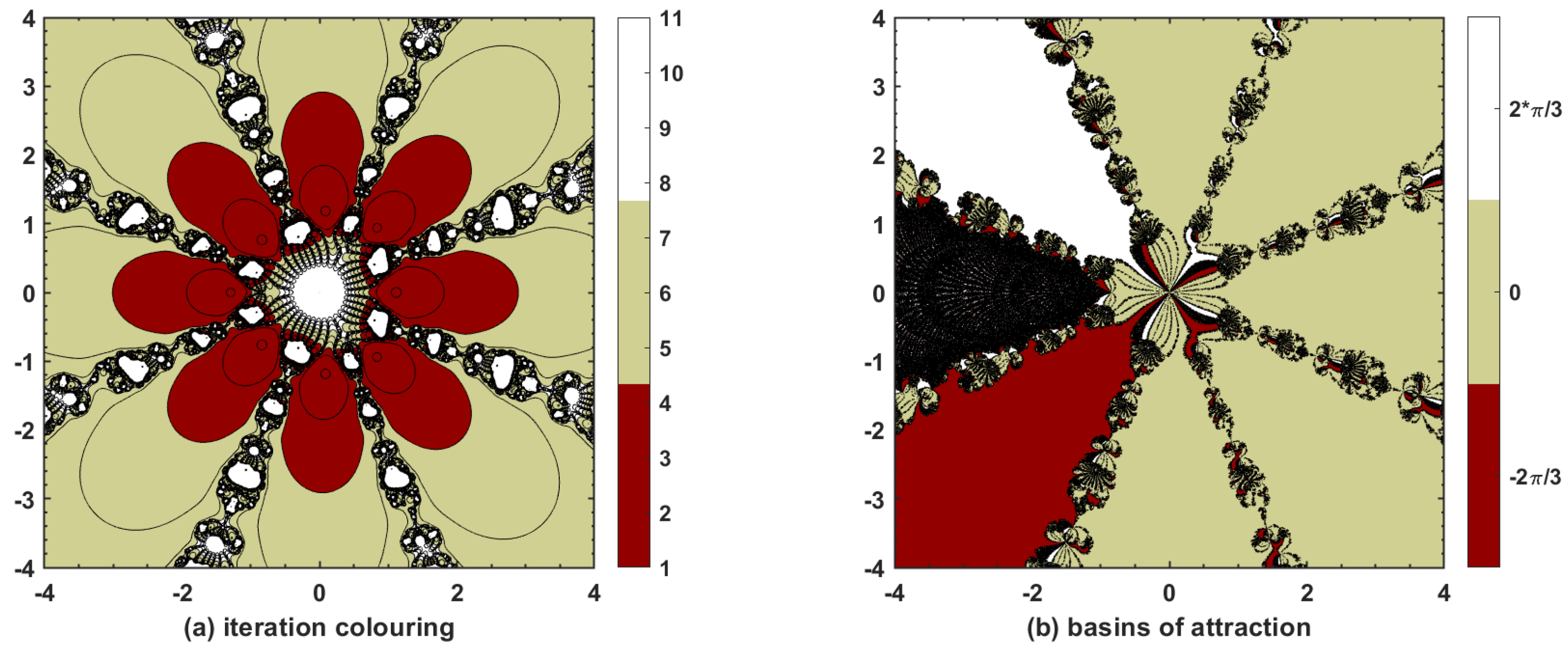
This research study is based on devising a new, highly effective three-step iterative method with tenth-order convergence. The convergence is proved theoretically via Taylor’s series expansion for single and multi-variable nonlinear equations, and the approximate computational order of convergence confirms such findings. Thus, the proposed method $P{M}_{10}$ is applicable not only to single nonlinear equations but also to nonlinear systems. Moreover, dynamical aspects of $P{M}_{10}$ are also explored with basins of attraction that show quite esthetic phase plane diagrams when applied to complex-valued functions, thereby proving the stability of the method when initial guesses are taken within the vicinity of the underlying nonlinear model. Finally, different types of nonlinear equations and systems, including those used in physical and natural sciences, are chosen to be tested with $P{M}_{10}$ and with various well-known optimal and non-optimal methods in the sense of King–Traub. In most of the cases, $P{M}_{10}$ is found to have better results, particularly when it comes to the number of iterations N to achieve required accuracy, ACOC, absolute error, and absolute functional value. It is also worthwhile to note that the proposed method always converges, irrespective of whether the initial guess passed to it lies near to or away from the approximate solution. Hence, $P{M}_{10}$ is a competitive iterative method with tenth-order convergence for solving nonlinear equations and systems.

We understand that methods of very high order are only of academic interest since approximations to the solutions of very high accuracy are not needed in practice. On the other hand, such methods are, to some extent, complicated and do not offer much of an increase in computational efficiency. Moreover, the method proposed in this article lies in the family of methods without memory, requiring the evaluation of three Jacobian matrices, and thereby becomes computationally expensive. To avoid computational complexity, we will propose, in future studies, a modification of the proposed method by replacing the first-order derivative with a suitable finite-difference approximation. In addition, the proposed method will also be analyzed for its semi-local convergence.

References

1. Ortega, J.M. Numerical Analysis: A Second Course; Society for Industrial and Applied Mathematics: Philadelphia, PA, USA, 1990. [Google Scholar]
2. Ham, Y.; Chun, C. A fifth-order iterative method for solving nonlinear equations. Appl. Math. Comput. 2007, 194, 287–290. [Google Scholar] [CrossRef]
3. Abro, H.A.; Shaikh, M.M. A new time-efficient and convergent nonlinear solver. Appl. Math. Comput. 2019, 355, 516–536. [Google Scholar] [CrossRef]
4. Cordero, A.; Torregrosa, J.R.; Vassileva, M.P. Design, Analysis, and Applications of Iterative Methods for Solving Nonlinear Systems. In Nonlinear Systems-Design, Analysis, Estimation and Control; Lee, D., Burg, T., Volos, C., Eds.; IntechOpen: Rijeka, Croatia, 2016. [Google Scholar] [CrossRef] [Green Version]
5. Hafiz, M.A.; Bahgat, M.S. An efficient two-step iterative method for solving system of nonlinear equations. J. Math. Res. 2012, 4, 28. [Google Scholar]
6. Noor, M.A.; Khan, W.A.; Hussain, A. A new modified Halley method without second derivatives for nonlinear equation. Appl. Math. Comput. 2007, 189, 1268–1273. [Google Scholar] [CrossRef]
7. Sharifi, M.; Babajee, D.K.R.; Soleymani, F. Finding the solution of nonlinear equations by a class of optimal methods. Comput. Math. Appl. 2012, 63, 764–774. [Google Scholar] [CrossRef] [Green Version]
8. Noor, M.A. Some iterative methods for solving nonlinear equations using homotopy perturbation method. Int. J. Comput. Math. 2010, 87, 141–149. [Google Scholar] [CrossRef]
9. Kung, H.T.; Traub, J.F. Optimal order of one-point and multipoint iteration. J. ACM (JACM) 1974, 21, 643–651. [Google Scholar] [CrossRef]
10. Householder, A.S. The Numerical Treatment of a Single Nonlinear Equation; McGraw-Hill: New York, NY, USA, 1970. [Google Scholar]
11. Bahgat, M.S.; Hafiz, M.A. Three-step iterative method with eighteenth order convergence for solving nonlinear equations. Int. J. Pure Appl. Math. 2014, 93, 85–94. [Google Scholar] [CrossRef]
12. Chun, C. Some fourth-order iterative methods for solving nonlinear equations. Appl. Math. Comput. 2008, 195, 454–459. [Google Scholar] [CrossRef]
13. Sharma, R.; Bahl, A. An optimal fourth order iterative method for solving nonlinear equations and its dynamics. J. Complex Anal. 2015, 2015, 259167. [Google Scholar] [CrossRef] [Green Version]
14. Geum, Y.H.; Kim, Y.I.; Neta, B. Constructing a family of optimal eighth-order modified Newton-type multiple-zero finders along with the dynamics behind their purely imaginary extraneous fixed points. J. Comput. Appl. Math. 2018, 333, 131–156. [Google Scholar] [CrossRef]
15. Qureshi, S.; Ramos, H.; Soomro, A.K. A New Nonlinear Ninth-Order Root-Finding Method with Error Analysis and Basins of Attraction. Mathematics 2021, 9, 1996. [Google Scholar] [CrossRef]
16. Ramos, H.; Monteiro, M.T.T. A new approach based on the Newton’s method to solve systems of nonlinear equations. J. Comput. Appl. Math. 2017, 318, 3–13. [Google Scholar] [CrossRef]
17. Ramos, H.; Vigo-Aguiar, J. The application of Newton’s method in vector form for solving nonlinear scalar equations where the classical Newton method fails. J. Comput. Appl. Math. 2015, 275, 228–237. [Google Scholar] [CrossRef]
18. Darvishi, M.T.; Barati, A. A third-order Newton-type method to solve systems of nonlinear equations. Appl. Math. Comput. 2007, 187, 630–635. [Google Scholar] [CrossRef]
19. Wang, X.; Liu, L. New eighth-order iterative methods for solving nonlinear equations. J. Comput. Appl. Math. 2010, 234, 1611–1620. [Google Scholar] [CrossRef] [Green Version]
20. Hu, Z.; Guocai, L.; Tian, L. An iterative method with ninth-order convergence for solving nonlinear equations. Int. J. Contemp. Math. Sci. 2011, 6, 17–23. [Google Scholar]
21. Hafiz, M.A.; Al-Goria, S.M. Solving nonlinear equations using a new tenth-and seventh-order methods free from second derivative. Int. J. Differ. Equ. Appl. 2013, 12. [Google Scholar]
22. Cordero, A.; Hueso, J.L.; Martínez, E.; Torregrosa, J.R. New modifications of Potra–Pták’s method with optimal fourth and eighth orders of convergence. J. Comput. Appl. Math. 2010, 234, 2969–2976. [Google Scholar] [CrossRef] [Green Version]
23. Lotfi, T.; Bakhtiari, P.; Cordero, A.; Mahdiani, K.; Torregrosa, J.R. Some new efficient multipoint iterative methods for solving nonlinear systems of equations. Int. J. Comput. Math. 2015, 92, 1921–1934. [Google Scholar] [CrossRef] [Green Version]
24. Cordero, A.; Hueso, J.L.; Martínez, E.; Torregrosa, J.R. A modified Newton-Jarratt’s composition. Numer. Algorithms 2010, 55, 87–99. [Google Scholar] [CrossRef]
25. Waseem, M.; Noor, M.A.; Noor, K.I. Efficient method for solving a system of nonlinear equations. Appl. Math. Comput. 2016, 275, 134–146. [Google Scholar] [CrossRef]
26. Noor, M.A.; Noor, K.I.; Al-Said, E.; Waseem, M. Some new iterative methods for nonlinear equations. Math. Probl. Eng. 2010, 2010, 198943. [Google Scholar] [CrossRef]
27. Hueso, J.L.; Martínez, E.; Torregrosa, J.R. Third and fourth order iterative methods free from second derivative for nonlinear systems. Appl. Math. Comput. 2009, 211, 190–197. [Google Scholar] [CrossRef]
28. Weerakoon, S.; Fernando, T.G.I. A variant of Newton’s method with accelerated third-order convergence. Appl. Math. Lett. 2000, 13, 87–93. [Google Scholar] [CrossRef]
29. Grau-Sánchez, M.; Gutiérrez, J.M. Zero-finder methods derived from Obreshkov’s techniques. Appl. Math. Comput. 2009, 215, 2992–3001. [Google Scholar] [CrossRef]
30. Petkovi´c, M.S. Remarks on “On a general class of multipoint root-finding methods of high computational efficiency”. SIAM J. Numer. Anal. 2011, 49, 1317–1319. [Google Scholar] [CrossRef]
31. Scott, M.; Neta, B.; Chun, C. Basin attractors for various methods. Appl. Math. Comput. 2011, 218, 2584–2599. [Google Scholar] [CrossRef]
32. Stewart, B.D. Attractor Basins of Various Root-Finding Methods; Naval Postgraduate School: Monterey, CA, USA, 2001. [Google Scholar]
33. Halley, E. A new, exact, and easy method of finding the roots of any equations generally, and that without any previous reduction. Philos. Trans. R. Soc. Lond. 1694, 18, 136–145. [Google Scholar]
34. Chen, H.; Zheng, X. Improved Newton Iterative Algorithm for Fractal Art Graphic Design. Complexity 2020, 2020, 6623049. [Google Scholar] [CrossRef]
35. Susanto, H.; Karjanto, N. Newton’s method’s basins of attraction revisited. Appl. Math. Comput. 2009, 215, 1084–1090. [Google Scholar] [CrossRef] [Green Version]
36. Tao, Y.; Madhu, K. Optimal Fourth, Eighth and Sixteenth Order Methods by Using Divided Difference Techniques and Their Basins of Attraction and Its Application. Mathematics 2019, 7, 322. [Google Scholar] [CrossRef] [Green Version]
37. Said Solaiman, O.; Hashim, I. Efficacy of optimal methods for nonlinear equations with chemical engineering applications. Math. Probl. Eng. 2019, 2019, 1728965. [Google Scholar] [CrossRef] [Green Version]
38. Khoury, R.; Harder, D.W. Numerical Methods and Modelling for Engineering; Springer: Berlin/Heidelberg, Germany, 2016; pp. 120–124. [Google Scholar]
39. Shacham, M. Numerical solution of constrained non-linear algebraic equations. Int. J. Numer. Methods Eng. 1986, 23, 1455–1481. [Google Scholar] [CrossRef]
40. Madhu, K.; Babajee, D.K.R.; Jayaraman, J. An improvement to double-step Newton method and its multi-step version for solving system of nonlinear equations and its applications. Numer. Algorithms 2017, 74, 593–607. [Google Scholar] [CrossRef]
41. Madhu, K.; Elango, A.; Landry, R., Jr.; Al-arydah, M.T. New multi-step iterative methods for solving systems of nonlinear equations and their application on GNSS pseudorange equations. Sensors 2020, 20, 5976. [Google Scholar] [CrossRef] [PubMed]
42. Burden, R.L.; Faires, J.D. Numerical Analysis; Brooks/Cole: Boston, MA, USA, 2010; Volume 7. [Google Scholar]
43. Amos, G.; Subramaniam, V. Numerical Methods for Engineers and Scientists: An Introduction with Applications Using MATLAB; Department of Mechanical Engineering, The Ohio State University: Columbus, OH, USA, 2014. [Google Scholar]
44. Chapra, S.C.; Canale, R.P. Numerical Methods for Engineers; McGraw-Hill Higher Education: Boston, MA, USA, 2010. [Google Scholar]
Figure 1. Flowchart of the proposed three-step method given in (8).
Fractalfract 05 00204 g001
Figure 2. Behavior of efficiency index of various iterative methods for increasing dimensions of the nonlinear problem.
Fractalfract 05 00204 g002
Figure 3. The polynomiographs by the proposed method P M 10 for P 1 ( z ) .
Fractalfract 05 00204 g003
Figure 4. The polynomiographs by the proposed method P M 10 for P 2 ( z ) .
Fractalfract 05 00204 g004
Figure 5. The polynomiographs by the proposed method P M 10 for P 3 ( z ) .
Fractalfract 05 00204 g005
Figure 6. The basins of attractions by the proposed method P M 10 for P 4 ( z ) .
Fractalfract 05 00204 g006
Figure 7. The basins of attractions by the proposed method P M 10 for P 5 ( z ) .
Fractalfract 05 00204 g007
Figure 8. The basins of attractions by the proposed method P M 10 for P 6 ( z ) .
Fractalfract 05 00204 g008