Hexagonal Grid Computation of the Derivatives of the Solution to the Heat Equation by Using Fourth-Order Accurate Two-Stage Implicit Methods

Abstract

We give fourth-order accurate implicit methods for the computation of the first-order spatial derivatives and second-order mixed derivatives involving the time derivative of the solution of first type boundary value problem of two dimensional heat equation. The methods are constructed based on two stages: At the first stage of the methods, the solution and its derivative with respect to time variable are approximated by using the implicit scheme in Buranay and Arshad in 2020. Therefore, $O\left(h^4+\tau \right)$ of convergence on constructed hexagonal grids is obtained that the step sizes in the space variables $x_1$, $x_2$ and in time variable are indicated by h, $\frac{\sqrt{3}}{2}h$ and $\tau$, respectively. Special difference boundary value problems on hexagonal grids are constructed at the second stages to approximate the first order spatial derivatives and the second order mixed derivatives of the solution. Further, $O\left(h^4+\tau \right)$ order of uniform convergence of these schemes are shown for $r=\frac{\omega \tau }{h^2}\ge \frac{1}{16}, \omega >0$. Additionally, the methods are applied on two sample problems.

1. Introduction

The modeling of numerous phenomena in diverse scientific fields leads us to consider conventional or fractional boundary value problems of time dependent differential equations on a modeling domain such as the first and second type boundary value problems to heat equation or diffusion equation. For example, the Brownian motion problem in statistics is modeled by heat equation via the Fokker–Planck equation (Adriaan Fokker [1] and Max Planck [2]). It is also named as the Kolmogorov forward equation, who discovered the concept in 1931, see in [3] independently. The stock market fluctuations represent one of the several important real-world applications of the mathematical model of Brownian motion. It was first given in the PhD thesis titled as “The theory of speculation”, by Louis Bachelier (see Mandelbrot and Hudson [4]) in 1900.

Another representative sample of problems that mathematical modeling brings about the heat equation is the image processing problems appearing through many applied sciences from archaeology to zoology. Examples of archaeological investigations include a camcorder for 3D underwater reconstruction of archeological objects in the study of Meline et al. [5]. Furthermore, a recent investigation by Woźniak and Polap [6] gave soft trees with neural components as image processing technique for archeological excavations. In zoology, a study of image reconstruction problem by the application of magnetic resonance imaging was given by Ziegler et al. [7] and in medical sciences as medical image reconstruction was studied in Zeng [8]. Furthermore, tomography, and medical and industrial applications are archetypal examples where substantial mathematical manipulation is required. In some cases, the aim is humble denoising or de-blurring. Witkin [9] and Koenderink [10] gave the modeling of blurring of an image by the heat equation. Later, a problem of solving the reverse heat equation known as de-blurring is studied in Rudin et al. [11] and Guichard and Morel [12].

Additionally, in mathematical biology, Wolpert [13,14] gave a phenomenological concept of pattern formation and differentiation known as positional information. The pre-programming of the cells for reacting to a chemical concentration and differentiate accordingly, into different kinds of cells such as cartilage cells was proposed. Afterwards, the animal coat patterns, pattern formation on growing domains as alligators, snakes and bacterial patterns were modeled by reaction diffusion equations in Murray [15]. Furthermore, therein, gliomas or glioblastomas, which are highly diffusive brain tumors, are analyzed and a mathematical model for the spatiotemporal dynamics of tumor growth was developed. Therefore, the basic model in dimensional form was given by the diffusion equation

$$\frac{\partial \overline{c}}{\partial \overline{t}}=\overline{\nabla }\mathbf{J}+\rho \overline{c},$$

(1)

where $\overline{c}(\overline{x},\overline{t})$ is the number of cells at a position $\overline{\mathbf{x}}$ and time $\overline{t},$$\rho$ represents the net rate of growth of cells including proliferation and death (or loss), and$\mathbf{J}$ diffusional flux of cells taken $\mathbf{J}=\overline{D}\overline{\nabla }\overline{c}$, where $\overline{D}\left(x\right)$ (distance${}^2$/time) is the diffusion coefficient of cells in brain tissue and $\overline{\nabla }$ is the gradient operator.

In general, finding analytical solutions of these modeled problems is a difficult task or even not possible. Approximations are needed when a mathematical model is switched to a numerical model. Finite difference methods (FDM) are a class of numerical techniques for solving differential equations that each derivative appearing in the partial differential equation has to be replaced by a suitable divided difference of function values at the chosen grid points, see Grossman et al. [16]. In the last decade, the use of advanced computers has led to the widespread use of FDM in modern numerical analysis. For example, recently, a study on fractional diffusion equation-based image denoising model using Crank–Nicholson and Grünwald Letnikov difference schemes (CN–GL) have been given in Abirami et al. [17]. Another example is the most recent investigation by Buranay and Nouman [18] in which computation of the solution to heat equation

$$\frac{\partial u}{\partial t}=\omega \left(\frac{{\partial }^{2}u}{\partial x_1^2}+\frac{{\partial }^{2}u}{\partial x_2^2}\right)+f\left(x_1,x_2,t\right),$$

(2)

on special polygons, where $\omega >0$ and f is the heat source by using implicit schemes defined on hexagonal grids was given. Therein, under some smoothness assumptions of the solution, two implicit methods were developed both on two layers with 14-point that has convergence orders of $O\left(h^2+{\tau }^2\right)$ and $O\left(h^4+\tau \right)$ accordingly to the solution on the grids. Besides the solution of the modeled problem, the high accurate computation of the derivatives of the solution are fundamental to determine some important phenomena of the considered model problem. Such as for the diffusion problem (1) the functions $\frac{\partial \overline{c}}{\partial \overline{t}}$ and $\mathbf{J}$ gives the rate of change of the cells and diffusional flux of cells, respectively.

In the literature, exhaustive studies exist for the approximation of the derivatives of the solution to Laplace’s equation under some smoothness conditions of the boundary functions and compatibility conditions. For the 2D Laplace equation, research was conducted by Volkov [19] and Dosiyev and Sadeghi [20]. For the 3D Laplace equation on a rectangular parallelepiped, studies were given by Volkov [21] and Dosiyev and Sadeghi [22], and recently by Dosiyev and Abdussalam [23], and Dosiyev and Sarikaya [24].

For the heat equation, the derivative of the solution of one-dimensional heat equation with respect to the space variable was given in Buranay and Farinola [25]. Within this paper, two implicit schemes were developed that converge to the corresponding exact spatial derivative with $O\left(h^2+\tau \right)$ and $O\left(h^2+{\tau }^2\right)$ accordingly. Most recently, in Buranay et al. [26] numerical methods using implicit schemes with hexagonal grids approximating the derivatives of the solution of (2) on a rectangle has been given. The smoothness condition $u\in C_{x,t}^{7+\alpha ,\frac{7+\alpha }{2}},$$0<\alpha <1$ in the Hölder space was required and uniform convergence on the grids to the respective spatial derivatives of $O\left(h^2+{\tau }^2\right)$ of accuracy for $r=\frac{\omega \tau }{h^2}$$\le \frac{3}{7}$ was proved.

In regard to the equilateral triangulation with a regular hexagonal support, we remark the research by Barrera et al. [27] where a new class of quasi-interpolant was constructed which has remarkable properties such as high order of regularity and polynomial reproduction. Furthermore, on the Delaunay triangulation, we mention the study by Guessab [28] that approximations of differentiable convex functions on arbitrary convex polytopes were given. Further, optimal approximations were computed by using efficient algorithms accessed by the set of barycentric coordinates generated by the Delaunay triangulation.

The motivation of the contributions of this research is the need of highly accurate and time-efficient numerical algorithms that compute the derivatives of the solution $u\left(x_1,x_2,t\right)$ to the heat Equation (2). The achievements of this study are summarized as follows.

• The first type boundary value problem (Dirichlet problem) for the heat Equation (2) on a rectangle D is considered. The smoothness of the solution u is taken from the Hölder space $C_{x,t}^{9+\alpha ,\frac{9+\alpha }{2}}\left({\overline{Q}}_T\right),$$0<\alpha <1$, where $x=\left(x_1,x_2\right)\in \overline{D},t\in \left[0,T\right]$ and $Q_T=D\times \left(0,T\right)$ also $\overline{D},$${\overline{Q}}_T$ denote the closure of $D,Q_T,$ respectively. At the first stage, an implicit scheme on hexagonal grids given in Buranay and Nouman [18] with $O\left(h^4+\tau \right)$ order of accuracy is used to approximate the solution $u\left(x_1,x_2,t\right).$ The step sizes h and $\frac{\sqrt{3}}{2}h$ are taken for the spatial variables $x_1$ and $x_2$, respectively, while $\tau$ is taken for the time variable. An analogous implicit method is also given to approximate the derivative of the solution with respect to time.
• At the second stages, computation of the first-order spatial derivatives and second-order mixed derivatives involving time derivatives of the solution $u\left(x_1,x_2,t\right)$ of (2) are developed. When $r=\frac{\omega \tau }{h^2}\ge \frac{1}{16}$ uniform convergence of the approximate derivative to the exact derivatives $\frac{\partial u}{\partial x_i},\frac{\partial u}{\partial t},$ and $\frac{{\partial }^{2}u}{\partial x_i\partial t},$$i=1,2$ with order $O\left(h^4+\tau \right)$ of accuracy on the hexagonal grids are proved.
• Numerical examples are given and for the solution of the obtained algebraic linear systems preconditioned conjugate gradient method is used. The incomplete block matrix factorization of the M-matrices given in Buranay and Iyikal [29] (see also Concus et al. [30], Axelsson [31]) is applied for the preconditioning.

2. Hexagonal Grid Approximation of the Heat Equation and the Rate of Change by Using Fourth Order Accurate Difference Schemes

Let $D=\left\{\left(x_1,x_2\right):0<x_1<a_1,0<x_2<a_2\right\}$ be a rectangle, where we require $a_2$ to be multiple of $\sqrt{3}$. Next, let ${\gamma }_j$, $j=1,2,3,4$, be the sides of D that starting from the side $x_1=0$ are labeled in anticlockwise direction. Furthermore, the boundary of D is shown by $S={\displaystyle \bigcup _{j=1}^4}{\gamma }_j$. Further, we indicate the closure of D by $\overline{D}=D\cup S$. Let $x=\left(x_1,x_2\right)$ and $Q_T=D\times \left(0,T\right),$ with the lateral surface $S_T=\left\{\left(x,t\right):x=\left(x_1,x_2\right)\in S,t\in \left[0,T\right]\right\}$ and ${\overline{Q}}_T$ is the closure of $Q_T$. Let s be a non-integer positive number, $C_{x,t}^{s,\frac{s}{2}}\left({\overline{Q}}_T\right)$ be the Banach space of functions $u\left(x,t\right)$ that are continuous in ${\overline{Q}}_T$ together with all derivatives of the form

$$\frac{{\partial }^{\xi +s_1+s_2}u}{\partial t^{\xi }\partial x_1^{s_1}\partial x_2^{s_2}}\mathrm{for}2\xi +s_1+s_2<s$$

(3)

with bounded norm

$${∥u∥}_{C_{x,t}^{s,\frac{s}{2}}\left({\overline{Q}}_T\right)}={⟨u⟩}_{Q_T}^{\left(s\right)}+\sum _{j=0}^{\left[s\right]}{⟨u⟩}_{Q_T}^{\left(j\right)},$$

(4)

where

$$\begin{array}{ccc}\hfill {⟨u⟩}_{Q_T}^{\left(j\right)}& =& \sum _{2\xi +s_1+s_2=j}\underset{{\overline{Q}}_T}{max}\left|\frac{{\partial }^{\xi +s_1+s_2}u}{\partial t^{\xi }\partial x_1^{s_1}\partial x_2^{s_2}}\right|,j=0,1,2,...,\left[s\right],\hfill \end{array}$$

(5)

$$\begin{array}{ccc}\hfill {⟨u⟩}_{Q_T}^{\left(s\right)}& =& {⟨u⟩}_x^{\left(s\right)}+{⟨u⟩}_t^{\left(\frac{s}{2}\right)},\hfill \end{array}$$

(6)

$$\begin{array}{ccc}\hfill {⟨u⟩}_x^{\left(s\right)}& =& \sum _{2r+s_1+s_2=\left[s\right]}{⟨\frac{{\partial }^{\xi +s_1+s_2}u}{\partial t^{\xi }\partial x_1^{s_1}\partial x_2^{s_2}}⟩}_x^{s-\left[s\right]},\hfill \end{array}$$

(7)

$$\begin{array}{ccc}\hfill {⟨u⟩}_t^{\left(\frac{s}{2}\right)}& =& \sum _{0<s-2\xi -s_1-s_2<2}{⟨\frac{{\partial }^{\xi +s_1+s_2}u}{\partial t^{\xi }\partial x_1^{s_1}\partial x_2^{s_2}}⟩}_t^{\frac{s-2\xi -s_1-s_2}{2}},\hfill \end{array}$$

(8)

further, ${⟨u⟩}_x^{\alpha },$${⟨u⟩}_t^{\beta }$ for $\alpha ,\beta \in \left(0,1\right)$ are defined as

$$\begin{array}{ccc}\hfill {⟨u⟩}_x^{\alpha }& =& \underset{\left(x,t\right),\left(x^{\prime },t\right)\in {\overline{Q}}_T}{sup}\frac{\left|u\left(x,t\right)-u\left(x^{\prime },t\right)\right|}{{\left|x-x^{\prime }\right|}^{\alpha }},\hfill \end{array}$$

(9)

$$\begin{array}{ccc}\hfill {⟨u⟩}_t^{\beta }& =& \underset{\left(x,t\right),\left(x,t^{\prime }\right)\in {\overline{Q}}_T}{sup}\frac{\left|u\left(x,t\right)-u\left(x,t^{\prime }\right)\right|}{{\left|t-t^{\prime }\right|}^{\beta }}.\hfill \end{array}$$

(10)

Volkov gave the differentiability properties of solutions of boundary value problems for the Laplace and Poisson equations on rectangle in the study [32]. On cylindrical domains with smooth boundary, the differentiability properties of solutions of the parabolic equations were given in Ladyženskaja et al. [33] and Friedman [34]. On regions with edges, Azzam and Kreyszig studied the smoothness of solutions of parabolic equations for the Dirichlet problem in [35] and for the mixed boundary value problem in [36].

2.1. Dirichlet Problem of Heat Equation and Difference Problem: Stage 1$\left(H^{4th}\left(u\right)\right)$

Our interest is the following problem for the heat equation:

• BVP$\left(u\right)$

$$\begin{array}{ccc}\hfill \frac{\partial u}{\partial t}& =& \omega \left(\frac{{\partial }^{2}u}{\partial x_1^2}+\frac{{\partial }^{2}u}{\partial x_2^2}\right)+f\left(x_1,x_2,t\right)\mathrm{on}{Q}_T,\hfill \\ \hfill u\left(x_1,x_2,0\right)& =& \phi \left(x_1,x_2\right)\mathrm{on}\overline{D},\hfill \\ \hfill u\left(x_1,x_2,t\right)& =& \varphi \left(x_1,x_2,t\right)\mathrm{on}{S}_T,\hfill \end{array}$$

(11)

where $\omega$ is positive constant. This problem is framed as first type (Dirichlet) boundary value problem.

We assume that the initial and boundary functions $\phi \left(x_1,x_2\right)$, $\varphi \left(x_1,x_2,t\right)$, respectively, also the heat source function $f\left(x_1,x_2,t\right)$ possess the necessary smoothness and satisfy the conditions that the problem (11) has unique solution $u\in C_{x,t}^{9+\alpha ,\frac{9+\alpha }{2}}\left({\overline{Q}}_T\right).$ We define hexagonal grids on D with the step size $h,$ such that $h=a_1/N_1$, and $N_1$ is positive integer and present this set by $D^h$ as

$$\begin{array}{ccc}\hfill D^h& =& \left\{x=(x_1,x_2)\in D:x_1=\frac{k^{\prime }-p^{\prime }}{2}h,x_2=\frac{\sqrt{3}(k^{\prime }+p^{\prime })}{2}h,\right.\hfill \\ & & \left.k^{\prime }=1,2,...;p^{\prime }=0\pm 1\pm 2,...\right\}\hfill \end{array}$$

(12)

Let ${\gamma }_j^h,j=1,...,4$ be the set of nodes on the interior of ${\gamma }_j$, and let ${\widehat{\gamma }}_j^h$=${\gamma }_{j-1}\cap {\gamma }_j$ be the $j-th$ vertex of D, $S^h={\displaystyle \bigcup _{j=1}^4}({\gamma }_j^h\cup {\widehat{\gamma }}_j^h),$${\overline{D}}^h=D^h\cup S^h.$ Further, we denote by $D^{*lh}$ and $D^{*rh}$ the set of interior nodes whose distance from the boundary is $\frac{h}{2}$, 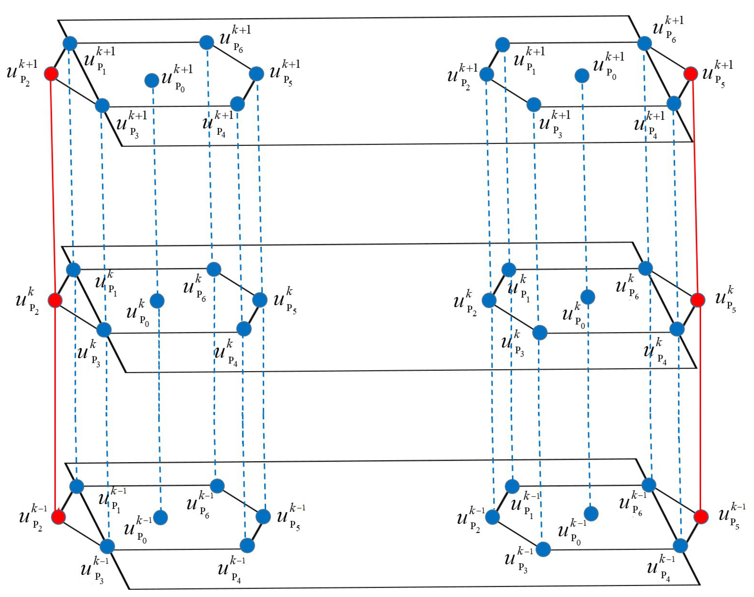thus the hexagon is irregular hexagon with a ghost point that emerges through the left ($x_1=0$) or right ($x_1=a_1$) side of the rectangle, respectively. The illustration of the exact solution at the irregular hexagons with a ghost point at time levels $t-\tau$, t and $t+\tau$ is given in Figure 1.

Figure 1. The illustration of the exact solution at the irregular hexagons with a ghost point at time levels $t-\tau$, t and $t+\tau$.

Further, we indicate by $D^{*h}=D^{*lh}\cup D^{*rh}$ and $D^{0h}=D^h\backslash D^{*h}$. Moreover, let

$$\begin{array}{ccc}\hfill {\gamma }_{\tau }& =& \left\{t_k=k\tau ,\tau =\frac{T}{M^{\prime }},k=1,...,M^{\prime }\right\},\hfill \end{array}$$

(13)

$$\begin{array}{ccc}\hfill {\overline{\gamma }}_{\tau }& =& \left\{t_k=k\tau ,\tau =\frac{T}{M^{\prime }},k=0,...,M^{\prime }\right\}.\hfill \end{array}$$

(14)

Next, we give the set of interior hexagonal points and the lateral surface points by

$$\begin{array}{ccc}\hfill D^h{\gamma }_{\tau }& =& D^h\times {\gamma }_{\tau }=\left\{\left(x,t\right):x\in D^h,t\in {\gamma }_{\tau }\right\},\hfill \end{array}$$

(15)

$$\begin{array}{ccc}\hfill S_T^h& =& S^h\times {\overline{\gamma }}_{\tau }=\left\{\left(x,t\right):x\in S^h,t\in {\overline{\gamma }}_{\tau }\right\},\hfill \end{array}$$

(16)

respectively. Let $D^{*lh}{\gamma }_{\tau }=D^{*lh}\times {\gamma }_{\tau }\subset D^h{\gamma }_{\tau }$ and $D^{*rh}{\gamma }_{\tau }=D^{*rh}\times {\gamma }_{\tau }\subset D^h{\gamma }_{\tau }$ and $D^{*h}{\gamma }_{\tau }=D^{*lh}{\gamma }_{\tau }\cup D^{*rh}{\gamma }_{\tau }$. Furthermore, $D^{0h}{\gamma }_{\tau }=D^h{\gamma }_{\tau }\backslash D^{*h}{\gamma }_{\tau }$ and $\overline{D^h{\gamma }_{\tau }}$ is the closure of $D^h{\gamma }_{\tau }.$ We denote the center of the hexagon by $P_0$ and $Patt\left(P_0\right)$ is the pattern of the hexagon consisting the neighboring points $P_i,i=1,...,6.$ Furthermore, the exact solution at the neighboring points $P_i,$$i=0,1,...,6$ for the time moment $t+\tau$ is presented by $u_{P_i}^{k+1}$, while $u_{P_A}^{k+1}$ is the value on the boundary point as given:

$$\begin{array}{ccc}\hfill u_{P_1}^{k+1}& =& u(x_1-\frac{h}{2},x_2+\frac{\sqrt{3}}{2}h,t+\tau ),u_{P_3}^{k+1}=u(x_1-\frac{h}{2},x_2-\frac{\sqrt{3}}{2}h,t+\tau )\hfill \\ \hfill u_{P_2}^{k+1}& =& u(x_1-h,x_2,t+\tau ),u_{P_5}^{k+1}=u(x_1+h,x_2,t+\tau )\hfill \\ \hfill u_{P_4}^{k+1}& =& u(x_1+\frac{h}{2},x_2-\frac{\sqrt{3}}{2}h,t+\tau ),u_{P_6}^{k+1}=u(x_1+\frac{h}{2},x_2+\frac{\sqrt{3}}{2}h,t+\tau )\hfill \\ \hfill u_{P_0}^{k+1}& =& u(x_1,x_2,t+\tau ),u_{P_A}^{k+1}=u(\widehat{p},x_2,t+\tau ),\hfill \end{array}$$

where $(\widehat{p},x_2,t+\tau )\in S_T^h$ and the value of $\widehat{p}=0$ if $P_0\in D^{*lh}{\gamma }_{\tau }$ and $\widehat{p}=a_1$ if $P_0\in D^{*rh}{\gamma }_{\tau }$. Moreover, $u_{h,\tau ,P_i}^{k+1},$$i=0,...,6,$ $u_{h,\tau ,P_A}^{k+1},$ present the numerical solution at the same space coordinates of $P_i,$$i=0,...,6$ and $P_A$ accordingly for time moments $t+\tau$. We also use the following notations in Table 1 to denote the values and partial derivatives of the heat source function f and $f_t=\frac{\partial f}{\partial t}$ with respect to the space variables.

Table 1. Basic notations for the heat source function f and $f_t$.

f	${\mathit{f}}_{\mathit{t}}$
$f_{P_0}^{k+1}=f(x_1,x_2,t+\tau )$	$f_{t,P_0}^{k+1}={\left.\frac{\partial f}{\partial t}\right|}_{(x_1,x_2,t+\tau )}$
$f_{P_A}^{k+1}=f(\widehat{p},x_2,t+\tau )$	$f_{t,P_A}^{k+1}={\left.\frac{\partial f}{\partial t}\right|}_{(\widehat{p},x_2,t+\tau )}$
$f_{P_A}^k=f(\widehat{p},x_2,t)$	$f_{t,P_A}^k={\left.\frac{\partial f}{\partial t}\right|}_{(\widehat{p},x_2,t)}$
${\partial }_{x_j}{f}_{P_A}^k={\left.\frac{\partial f}{\partial x_j}\right|}_{(\widehat{p},x_2,t)},$$j=1,2$	${\partial }_{x_j}{f}_{t,P_A}^k={\left.\frac{{\partial }^{2}f}{\partial x_j\partial t}\right|}_{(\widehat{p},x_2,t)},$$j=1,2$
${\partial }_{x_j}^2{f}_{P_0}^{k+1}={\left.\frac{{\partial }^{2}f}{\partial x_j^2}\right|}_{(x_1,x_2,t+\tau )},$$j=1,2$	${\partial }_{x_j}^2{f}_{t,P_0}^{k+1}={\left.\frac{{\partial }^{3}f}{\partial x_j^2\partial t}\right|}_{(x_1,x_2,t+\tau )},$$j=1,2$
${\partial }_{x_2}^2{\partial }_{x_1}{f}_{P_0}^{k+1}={\left.\frac{{\partial }^{3}f}{\partial x_2^2\partial x_1}\right|}_{(x_1,x_2,t+\tau )}$	${\partial }_{x_2}^2{\partial }_{x_1}{f}_{t,P_0}^{k+1}={\left.\frac{{\partial }^{4}f}{\partial x_2^2\partial x_1\partial t}\right|}_{(x_1,x_2,t+\tau )}$
${\partial }_{x_1}^2{\partial }_{x_2}{f}_{P_0}^{k+1}={\left.\frac{{\partial }^{3}f}{\partial x_1^2\partial x_2}\right|}_{(x_1,x_2,t+\tau )}$	${\partial }_{x_1}^2{\partial }_{x_2}{f}_{t,P_0}^{k+1}={\left.\frac{{\partial }^{4}f}{\partial x_1^2\partial x_2\partial t}\right|}_{(x_1,x_2,t+\tau )}$

For computing numerically the solution of the BVP$\left(u\right)$ we use the following difference problem given in Buranay and Arshad [18] and call this Stage 1$\left(H^{4th}\left(u\right)\right)$.

• Stage 1$\left(H^{4th}\left(u\right)\right)$

$$\begin{array}{ccc}\hfill {\tilde{\mathsf{\Theta }}}_{h,\tau }{u}_{h,\tau }^{k+1}& =& {\tilde{\mathsf{\Lambda }}}_{h,\tau }{u}_{h,\tau }^k+\tilde{\psi }\mathrm{on}{D}^{0h}{\gamma }_{\tau },\hfill \\ \hfill {\tilde{\mathsf{\Theta }}}_{h,\tau }^{*}{u}_{h,\tau }^{k+1}& =& {\tilde{\mathsf{\Lambda }}}_{h,\tau }^{*}{u}_{h,\tau }^k+{\tilde{\mathsf{\Gamma }}}_{h,\tau }^{*}\varphi +{\tilde{\psi }}^{*}\mathrm{on}{D}^{*h}{\gamma }_{\tau },\hfill \\ \hfill u_{h,\tau }& =& \phi \left(x_1,x_2\right),t=0\mathrm{on}{\overline{D}}^h,\hfill \\ \hfill u_{h,\tau }& =& \varphi \left(x_1,x_2,t\right)\mathrm{on}{S}_T^h,\hfill \end{array}$$

(17)

$k=0,...,M^{\prime }-1,$ where $\phi ,\varphi$ are the initial and boundary functions in (11), respectively, also

$$\begin{array}{ccc}\hfill \tilde{\psi }& =& f_{P_0}^{k+1}+\frac{1}{16}{h}^2\left({\partial }_{x_1}^2{f}_{P_0}^{k+1}+{\partial }_{x_2}^2{f}_{P_0}^{k+1}\right),\hfill \\ \hfill {\tilde{\psi }}^{*}& =& \frac{h^2}{96\tau \omega }{f}_{P_A}^{k+1}-\frac{h^2}{96\tau \omega }{f}_{P_A}^k-\frac{1}{6}{f}_{P_A}^{k+1}+f_{P_0}^{k+1}\hfill \end{array}$$

(18)

$$\begin{array}{ccc}& & +\frac{1}{16}{h}^2\left({\partial }_{x_1}^2{f}_{P_0}^{k+1}+{\partial }_{x_2}^2{f}_{P_0}^{k+1}\right),\hfill \end{array}$$

(19)

$${\tilde{\mathsf{\Theta }}}_{h,\tau }{u}^{k+1}=\left(\frac{3}{4\tau }+\frac{4\omega }{h^2}\right)u_{P_0}^{k+1}+\left(\frac{1}{24\tau }-\frac{2\omega }{3h^2}\right)\sum _{i=1}^6{u}_{P_i}^{k+1},$$

(20)

$${\tilde{\mathsf{\Lambda }}}_{h,\tau }{u}^k=\frac{3}{4\tau }{u}_{P_0}^k+\frac{1}{24\tau }\sum _{i=1}^6{u}_{P_i}^k,$$

(21)

$$\begin{array}{ccc}\hfill {\tilde{\mathsf{\Theta }}}_{h,\tau }^{*}{u}^{k+1}& =& \left(\frac{17}{24\tau }+\frac{14\omega }{3h^2}\right)u_{P_0}^{k+1}+\left(\frac{1}{24\tau }-\frac{2\omega }{3h^2}\right)\left(u(p,x_2+\frac{\sqrt{3}}{2}h,t+\tau )\right.\hfill \\ & & \left.+u(p,x_2-\frac{\sqrt{3}}{2}h,t+\tau )+u(p+\eta ,x_2,t+\tau )\right),\hfill \end{array}$$

(22)

$$\begin{array}{ccc}\hfill {\tilde{\mathsf{\Gamma }}}_{h,\tau }^{*}\varphi & =& \left(-\frac{1}{36\tau }+\frac{4\omega }{9h^2}\right)\left(\varphi (\widehat{p},x_2+\frac{\sqrt{3}}{2}h,t+\tau )+\varphi (\widehat{p},x_2-\frac{\sqrt{3}}{2}h,t+\tau )\right)\hfill \\ & & +\left(\frac{1}{18\tau }+\frac{16\omega }{9h^2}\right)\varphi (\widehat{p},x_2,t+\tau )-\frac{1}{18\tau }\varphi (\widehat{p},x_2,t)\hfill \\ & & +\frac{1}{36\tau }\left(\varphi (\widehat{p},x_2+\frac{\sqrt{3}}{2}h,t)+\varphi (\widehat{p},x_2-\frac{\sqrt{3}}{2}h,t)\right),\hfill \end{array}$$

(23)

$$\begin{array}{ccc}\hfill {\tilde{\mathsf{\Lambda }}}_{h,\tau }^{*}{u}^k& =& \frac{17}{24\tau }{u}_{P_0}^k+\frac{1}{24\tau }\left(u(p,x_2+\frac{\sqrt{3}}{2}h,t)\right.\hfill \\ & & \left.+u(p,x_2-\frac{\sqrt{3}}{2}h,t)+u(p+\eta ,x_2,t)\right),\hfill \end{array}$$

(24)

and

$$\left\{\begin{array}{c}p=h,\widehat{p}=0,\eta =\frac{h}{2}\mathrm{if}{P}_0\in D^{*lh}{\gamma }_{\tau },\\ p=a_1-h,\widehat{p}=a_1,\eta =-\frac{h}{2}\mathrm{if}{P}_0\in D^{*rh}{\gamma }_{\tau }.\end{array}\right.$$

(25)

2.2. Dirichlet Problem for the Rate of Change and Difference Problem: Stage 1$\left(H^{4th}\left(\frac{\partial u}{\partial t}\right)\right)$

Further, for the computation of $\frac{\partial u}{\partial t}$, we construct the next boundary value problem denoted by $u_t=\frac{\partial u}{\partial t}$ which defines the rate of change function

• BVP$\left(\frac{\partial u}{\partial t}\right)$

$$\begin{array}{ccc}\hfill \frac{\partial u_t}{\partial t}& =& \omega \left(\frac{{\partial }^2{u}_t}{\partial x_1^2}+\frac{{\partial }^2{u}_t}{\partial x_2^2}\right)+f_t\left(x_1,x_2,t\right)\mathrm{on}{Q}_T,\hfill \\ \hfill u_t\left(x_1,x_2,0\right)& =& \widehat{\phi }(x_1,x_2)\mathrm{on}\overline{D},\hfill \\ \hfill u_t\left(x_1,x_2,t\right)& =& {\varphi }_t\left(x_1,x_2,t\right)\mathrm{on}{S}_T,\hfill \end{array}$$

(26)

where

$$\begin{array}{ccc}\hfill f_t& =& \frac{\partial f\left(x_1,x_2,t\right)}{\partial t},\hfill \\ \hfill \widehat{\phi }& =& \omega \left(\frac{{\partial }^2\phi }{\partial x_1^2}+\frac{{\partial }^2\phi }{\partial x_2^2}\right)+f\left(x_1,x_2,0\right),\hfill \\ \hfill {\varphi }_t& =& \frac{\partial \varphi \left(x_1,x_2,t\right)}{\partial t},\hfill \end{array}$$

(27)

and $\phi ,\varphi$ are the initial and boundary functions in (11).

Assuming $u_t\in C_{x,t}^{7+\alpha ,\frac{7+\alpha }{2}}\left({\overline{Q}}_T\right)$, fourth-order accurate implicit schemes for the solution of the BVP$\left(\frac{\partial u}{\partial t}\right)$ is proposed with the following difference problem. This stage is called Stage 1$\left(H^{4th}\left(\frac{\partial u}{\partial t}\right)\right)$.

Stage 1$\left(H^{4th}\left(\frac{\partial u}{\partial t}\right)\right)$

$$\begin{array}{ccc}\hfill {\tilde{\mathsf{\Theta }}}_{h,\tau }{u}_{t,h,\tau }^{k+1}& =& {\tilde{\mathsf{\Lambda }}}_{h,\tau }{u}_{t,h,\tau }^k+{\tilde{\psi }}_t\mathrm{on}{D}^{0h}{\gamma }_{\tau },\hfill \\ \hfill {\tilde{\mathsf{\Theta }}}_{h,\tau }^{*}{u}_{t,h,\tau }^{k+1}& =& {\tilde{\mathsf{\Lambda }}}_{h,\tau }^{*}{u}_{t,h,\tau }^k+{\tilde{\mathsf{\Gamma }}}_{h,\tau }^{*}{\varphi }_t+{\tilde{\psi }}_t^{*}\mathrm{on}{D}^{*h}{\gamma }_{\tau },\hfill \\ \hfill u_{t,h,\tau }& =& \widehat{\phi },t=0\mathrm{on}{\overline{D}}^h,\hfill \\ \hfill u_{t,h,\tau }& =& {\varphi }_t\left(x_1,x_2,t\right)\mathrm{on}{S}_T^h,\hfill \end{array}$$

(28)

$k=0,...,M^{\prime }-1,$ where the operators ${\tilde{\mathsf{\Theta }}}_{h,\tau },$ ${\tilde{\mathsf{\Lambda }}}_{h,\tau },{\tilde{\mathsf{\Theta }}}_{h,\tau }^{*},$${\tilde{\mathsf{\Gamma }}}_{h,\tau }^{*}$ and ${\tilde{\mathsf{\Lambda }}}_{h,\tau }^{*}$ are presented in (20)–(24), respectively, and

$$\begin{array}{ccc}\hfill {\tilde{\psi }}_t& =& f_{t,P_0}^{k+1}+\frac{1}{16}{h}^2\left({\partial }_{x_1}^2{f}_{t,P_0}^{k+1}+{\partial }_{x_2}^2{f}_{t,P_0}^{k+1}\right),\hfill \\ \hfill {\tilde{\psi }}_t^{*}& =& \frac{h^2}{96\tau \omega }{f}_{t,P_A}^{k+1}-\frac{h^2}{96\tau \omega }{f}_{t,P_A}^k-\frac{1}{6}{f}_{t,P_A}^{k+1}+f_{t,P_0}^{k+1}\hfill \end{array}$$

(29)

$$\begin{array}{ccc}& & +\frac{1}{16}{h}^2\left({\partial }_{x_1}^2{f}_{t,P_0}^{k+1}+{\partial }_{x_2}^2{f}_{t,P_0}^{k+1}\right).\hfill \end{array}$$

(30)

2.3. $M-$Matrices and Convergence of Finite Difference Schemes in Stage 1$\left(H^{4th}\left(u\right)\right)$ and Stage 1$\left(H^{4th}\left(\frac{\partial u}{\partial t}\right)\right)$

Let $A=\left[a_{i,j}\right]$ and $B=\left[b_{i,j}\right]$, $i=1,2,...,N$ and $j=1,2,...,N$ be real matrices. We denote by $A>0$ ($A\ge 0$) if $a_{i,j}>0$ ($a_{i,j}\ge 0$) for all $i,j$. Also $A<B$ ($A\le B$) if $a_{i,j}<b_{i,j}$ ($a_{i,j}\le b_{i,j}$). Analogous notation is also used for the vectors. Further, let w be a vector with coordinates $w_j,j=1,2,...,N,$ the vector with coordinates $\left|w_j\right|$ is denoted by $\left|w\right|.$ For a fixed time level $k\ge 0$ we present the Equations (17) and (28) in matrix form with N unknown interior grid points $L_j,$$j=1,2,...,N,$ labeled using standard ordering as

$$\begin{array}{ccc}\hfill \tilde{A}{\tilde{u}}^{k+1}& =& \tilde{B}{\tilde{u}}^k+\tau {\tilde{q}}_u^k,\hfill \\ \hfill \tilde{A}{\tilde{u}}_t^{k+1}& =& \tilde{B}{\tilde{u}}_t^k+\tau {\tilde{q}}_{u_t}^k,\hfill \end{array}$$

(31)

respectively, where $\tilde{A},\tilde{B}\in R^{N\times N}$ and ${\tilde{u}}^k,{\tilde{q}}_u^k,{\tilde{u}}_t^k,{\tilde{q}}_{u_t}^k\in R^N$ and

$$\begin{array}{ccc}\hfill \tilde{A}& =& \left({\breve{E}}_1+\frac{1}{24}Inc+\frac{\omega \tau }{h^2}\tilde{C}\right),\tilde{B}=\left({\breve{E}}_1+\frac{1}{24}Inc\right),\hfill \end{array}$$

(32)

$$\begin{array}{ccc}\hfill \tilde{C}& =& {\breve{E}}_2-\frac{2}{3}Inc\in R^{N\times N}.\hfill \end{array}$$

(33)

and $Inc$ is the neighboring topology matrix, ${\breve{E}}_1,{\breve{E}}_2$ are diagonal matrices with entries

$${\left[{\breve{E}}_1\right]}_{j,j}=\left\{\begin{array}{c}\frac{3}{4}\mathrm{if}{L}_j\in D^{0h}{\gamma }_{\tau }\\ \frac{17}{24}\mathrm{if}{L}_j\in D^{*h}{\gamma }_{\tau }\end{array}\right.,j=1,2,...,N,$$

(34)

$${\left[{\breve{E}}_2\right]}_{j,j}=\left\{\begin{array}{c}4\mathrm{if}{L}_j\in D^{0h}{\gamma }_{\tau }\\ \frac{14}{3}\mathrm{if}{L}_j\in D^{*h}{\gamma }_{\tau }\end{array}\right.,j=1,2,...,N,$$

(35)

respectively (see Buranay and Arshad [18]).

Lemma 1.

(Buranay and Arshad [18]) (a) The matrices $\tilde{A}$ and $\tilde{B}$ in (31) are symmetric positive definite (spd) matrices

(b) $\widehat{A}=I+\frac{\omega \tau }{h^2}{\tilde{B}}^{-1}\tilde{C}$ is spd matrix and ${∥{\widehat{A}}^{-1}∥}_2<1$.

Lemma 2.

The matrix $\tilde{A}$ in (31) is nonsingular $M-$matrix for $r=\frac{\omega \tau }{h^2}\ge \frac{1}{16}.$

Proof. 

Taking into consideration Lemma 1, the matrix $\tilde{A}$ is a spd matrix. Further, using the Equations (32)–(35), $\tilde{A}$ is strictly diagonally dominant matrix with positive diagonal entries. Furthermore, off-diagonal entries are non-positive for $r=\frac{\omega \tau }{h^2}\ge \frac{1}{16}.$ Therefore, it is nonsingular $M-$matrix. □

Let

$$\begin{array}{ccc}\hfill {\xi }_{h,\tau }^u& =& u_{h,\tau }-u\mathrm{on}\overline{D^h{\gamma }_{\tau }}\hfill \end{array}$$

(36)

$$\begin{array}{ccc}\hfill {\xi }_{h,\tau }^{u_t}& =& u_{t,h,\tau }-u_t\mathrm{on}\overline{D^h{\gamma }_{\tau }}\hfill \end{array}$$

(37)

From (17) and (36) the error function (36) satisfies the following system as given in Buranay and Arshad: [18]

$$\begin{array}{ccc}\hfill {\tilde{\mathsf{\Theta }}}_{h,\tau }{\xi }_{h,\tau }^{u,k+1}& =& {\tilde{\mathsf{\Lambda }}}_{h,\tau }{\xi }_{h,\tau }^{u,k}+{\tilde{\mathsf{\Psi }}}_1^{u,k}\mathrm{on}{D}^{0h}{\gamma }_{\tau },\hfill \\ \hfill {\tilde{\mathsf{\Theta }}}_{h,\tau }^{*}{\xi }_{h,\tau }^{u,k+1}& =& {\tilde{\mathsf{\Lambda }}}_{h,\tau }^{*}{\xi }_{h,\tau }^{u,k}+{\tilde{\mathsf{\Psi }}}_2^{u,k}\mathrm{on}{D}^{*h}{\gamma }_{\tau },\hfill \\ \hfill {\xi }_{h,\tau }^u& =& 0,t=0\mathrm{on}{\overline{D}}^h,\hfill \\ \hfill {\xi }_{h,\tau }^u& =& 0\mathrm{on}{S}_T^h,\hfill \end{array}$$

(38)

where

$$\begin{array}{ccc}\hfill {\tilde{\mathsf{\Psi }}}_1^{u,k}& =& {\tilde{\mathsf{\Lambda }}}_{h,\tau }{u}^k-{\tilde{\mathsf{\Theta }}}_{h,\tau }{u}^{k+1}+\tilde{\psi },\hfill \end{array}$$

(39)

$$\begin{array}{ccc}\hfill {\tilde{\mathsf{\Psi }}}_2^{u,k}& =& {\tilde{\mathsf{\Lambda }}}_{h,\tau }^{*}{u}^k-{\tilde{\mathsf{\Theta }}}_{h,\tau }^{*}{u}^{k+1}+{\tilde{\mathsf{\Gamma }}}_{h,\tau }^{*}\varphi +{\tilde{\psi }}^{*},\hfill \end{array}$$

(40)

and $\tilde{\psi },{\tilde{\psi }}^{*}$ and $\varphi$ are presented in (17). Analogously, using (28) and (37) the error function (37) satisfies the following system:

$$\begin{array}{ccc}\hfill {\tilde{\mathsf{\Theta }}}_{h,\tau }{\xi }_{h,\tau }^{u_t,k+1}& =& {\tilde{\mathsf{\Lambda }}}_{h,\tau }{\xi }_{h,\tau }^{u_t,k}+{\tilde{\mathsf{\Psi }}}_1^{u_t,k}\mathrm{on}{D}^{0h}{\gamma }_{\tau },\hfill \\ \hfill {\tilde{\mathsf{\Theta }}}_{h,\tau }^{*}{\xi }_{h,\tau }^{u_t,k+1}& =& {\tilde{\mathsf{\Lambda }}}_{h,\tau }^{*}{\xi }_{h,\tau }^{u_t,k}+{\tilde{\mathsf{\Psi }}}_2^{u_t,k}\mathrm{on}{D}^{*h}{\gamma }_{\tau },\hfill \\ \hfill {\xi }_{h,\tau }^{u_t}& =& 0,t=0\mathrm{on}{\overline{D}}^h,\hfill \\ \hfill {\xi }_{h,\tau }^{u_t}& =& 0\mathrm{on}{S}_T^h,\hfill \end{array}$$

(41)

where

$$\begin{array}{ccc}\hfill {\tilde{\mathsf{\Psi }}}_1^{u_t,k}& =& {\tilde{\mathsf{\Lambda }}}_{h,\tau }{u}_t^k-{\tilde{\mathsf{\Theta }}}_{h,\tau }{u}_t^{k+1}+{\tilde{\psi }}_t,\hfill \end{array}$$

(42)

$$\begin{array}{ccc}\hfill {\tilde{\mathsf{\Psi }}}_2^{u_t,k}& =& {\tilde{\mathsf{\Lambda }}}_{h,\tau }^{*}{u}_t^k-{\tilde{\mathsf{\Theta }}}_{h,\tau }^{*}{u}_t^{k+1}+{\tilde{\mathsf{\Gamma }}}_{h,\tau }^{*}{\varphi }_t+{\tilde{\psi }}_t^{*},\hfill \end{array}$$

(43)

and ${\varphi }_t,{\tilde{\psi }}_t$, and ${\tilde{\psi }}_t^{*}$ are the given functions in (27), (29) and (30) respectively.

Further, the following systems are considered:

$$\begin{array}{ccc}\hfill {\tilde{\mathsf{\Theta }}}_{h,\tau }{\widehat{w}}_{h,\tau }^{k+1}& =& {\tilde{\mathsf{\Lambda }}}_{h,\tau }{\widehat{w}}_{h,\tau }^k+{\widehat{\kappa }}_1^k\mathrm{on}{D}^{0h}{\gamma }_{\tau },\hfill \\ \hfill {\tilde{\mathsf{\Theta }}}_{h,\tau }^{*}{\widehat{w}}_{h,\tau }^{k+1}& =& {\tilde{\mathsf{\Lambda }}}_{h,\tau }^{*}{\widehat{w}}_{h,\tau }^k+{\tilde{\mathsf{\Gamma }}}_{h,\tau }^{*}{\widehat{w}}_{\varphi ,h,\tau }+{\widehat{\kappa }}_2^k\mathrm{on}{D}^{*h}{\gamma }_{\tau },\hfill \\ \hfill {\widehat{w}}_{h,\tau }& =& {\widehat{w}}_{\phi ,h,\tau },t=0\mathrm{on}{\overline{D}}^h,\hfill \\ \hfill {\widehat{w}}_{h,\tau }& =& {\widehat{w}}_{\varphi ,h,\tau }\mathrm{on}{S}_T^h,\hfill \end{array}$$

(44)

$$\begin{array}{ccc}\hfill {\tilde{\mathsf{\Theta }}}_{h,\tau }{\overline{w}}_{h,\tau }^{k+1}& =& {\tilde{\mathsf{\Lambda }}}_{h,\tau }{\overline{w}}_{h,\tau }^k+{\overline{\kappa }}_1^k\mathrm{on}{D}^{0h}{\gamma }_{\tau },\hfill \\ \hfill {\tilde{\mathsf{\Theta }}}_{h,\tau }^{*}{\overline{w}}_{h,\tau }^{k+1}& =& {\tilde{\mathsf{\Lambda }}}_{h,\tau }^{*}{\overline{w}}_{h,\tau }^k+{\tilde{\mathsf{\Gamma }}}_{h,\tau }^{*}{\overline{w}}_{\varphi ,h,\tau }+{\overline{\kappa }}_2^k\mathrm{on}{D}^{*h}{\gamma }_{\tau },\hfill \\ \hfill {\overline{w}}_{h,\tau }& =& {\overline{w}}_{\phi ,h,\tau },t=0\mathrm{on}{\overline{D}}^h,\hfill \\ \hfill {\overline{w}}_{h,\tau }& =& {\overline{w}}_{\varphi ,h,\tau }\mathrm{on}{S}_T^h,\hfill \end{array}$$

(45)

for $k=0,...,M^{\prime }-1,$ where ${\widehat{\kappa }}_1^k,{\widehat{\kappa }}_2^k$ and ${\overline{\kappa }}_1^k,{\overline{\kappa }}_2^k$ are given functions. The algebraic systems (44) and (45) at a fixed time level $k\ge 0$ may be given in matrix representation as

$$\begin{array}{ccc}\hfill \tilde{A}{\widehat{w}}^{k+1}& =& \tilde{B}{\widehat{w}}^k+\tau {\widehat{\kappa }}^k,\hfill \end{array}$$

(46)

$$\begin{array}{ccc}\hfill \tilde{A}{\overline{w}}^{k+1}& =& \tilde{B}{\overline{w}}^k+\tau {\overline{\kappa }}^k,\hfill \end{array}$$

(47)

accordingly. In these equations, ${\widehat{w}}^k,{\overline{w}}^k,{\widehat{\kappa }}^k,{\overline{\kappa }}^k\in R^N$ and the matrices $\tilde{A}$ and $\tilde{B}$ are given in (32).

Lemma 3.

Let the solutions of (46) and (47) be presented by ${\widehat{w}}^{k+1}$ and ${\overline{w}}^{k+1}$, respectively, for $r=\frac{\omega \tau }{h^2}\ge \frac{1}{16}$. If

$$\begin{array}{ccc}\hfill {\overline{w}}^0& \ge & 0and{\overline{\kappa }}^k\ge 0\hfill \end{array}$$

(48)

$$\begin{array}{ccc}\hfill \left|{\widehat{w}}^0\right|& \le & {\overline{w}}^0,\hfill \end{array}$$

(49)

$$\begin{array}{ccc}\hfill \left|{\widehat{\kappa }}^k\right|& \le & {\overline{\kappa }}^k,\hfill \end{array}$$

(50)

for $k=0,...,M^{\prime }-1$ then

$$\left|{\widehat{w}}^{k+1}\right|\le {\overline{w}}^{k+1},k=0,...,M^{\prime }-1,$$

(51)

Proof. 

From Lemma 2, when $r=\frac{\omega \tau }{h^2}\ge \frac{1}{16}$ the matrix $\tilde{A}$ is nonsingular $M-$matrix therefore, ${\tilde{A}}^{-1}\ge 0.$ Furthermore, from (32) $\tilde{B}\ge 0$ and using (48) it follows that ${\overline{\kappa }}^k\ge 0,$$k=0,...,M^{\prime }-1$ and ${\overline{w}}^0\ge 0.$ Further, assuming ${\overline{w}}^k\ge 0$ and from induction we achieve

$${\overline{w}}^{k+1}={\tilde{A}}^{-1}\tilde{B}{\overline{w}}^k+\tau A^{-1}{\overline{\kappa }}^k\ge 0,$$

(52)

which gives ${\overline{w}}^{k+1}\ge 0$ for $k=0,...,M^{\prime }-1.$ Next, assume that $\left|{\widehat{w}}^k\right|\le {\overline{w}}^k$ using (46)–(50), and by induction it follows that

$$\begin{array}{ccc}\hfill {\widehat{w}}^{k+1}& =& {\tilde{A}}^{-1}\tilde{B}{\widehat{w}}^k+\tau {\tilde{A}}^{-1}{\widehat{\kappa }}^k\hfill \end{array}$$

(53)

$$\begin{array}{ccc}\hfill \left|{\widehat{w}}^{k+1}\right|& \le & {\tilde{A}}^{-1}\tilde{B}\left|{\widehat{w}}^k\right|+\tau {\tilde{A}}^{-1}\left|{\widehat{\kappa }}^k\right|\hfill \\ & \le & {\tilde{A}}^{-1}\tilde{B}{\overline{w}}^k+\tau {\tilde{A}}^{-1}{\overline{\kappa }}^k={\overline{w}}^{k+1},\mathrm{for}k=0,...,M^{\prime }-1.\hfill \end{array}$$

(54)

□

Remark 1.

Writing the implicit schemes on hexagonal grids for the problems (17) and (28) in the canonical form it follows that the maximum principle holds when $r=\frac{\omega \tau }{h^2}\ge \frac{1}{16}.$ Further, Lemma 3 is the consequence of comparison theorem (see Chapter 4, Section 4.2 Theorem 1 and Theorem 2 in Samarskii [37]) applied to the systems (44) and (45).

Additionally, let

$$\begin{array}{ccc}\hfill {\mu }_1\left(u\right)& =& max\left\{\underset{{\overline{Q}}_T}{max}\left|\frac{{\partial }^{5}u}{\partial x_1^4\partial t}\right|,\underset{{\overline{Q}}_T}{max}\left|\frac{{\partial }^{5}u}{\partial x_2^4\partial t}\right|,\underset{{\overline{Q}}_T}{max}\left|\frac{{\partial }^{5}u}{\partial x_1^2\partial x_2^2\partial t}\right|\right.,\hfill \\ & & \left.\underset{{\overline{Q}}_T}{max}\left|\frac{{\partial }^{6}u}{\partial x_1^4\partial x_2^2}\right|,\underset{{\overline{Q}}_T}{max}\left|\frac{{\partial }^{6}u}{\partial x_1^2\partial x_2^4}\right|,\underset{{\overline{Q}}_T}{max}\left|\frac{{\partial }^{6}u}{\partial x_1^6}\right|,\underset{{\overline{Q}}_T}{max}\left|\frac{{\partial }^{6}u}{\partial x_2^6}\right|\right\},\hfill \end{array}$$

(55)

$$\begin{array}{ccc}\hfill {\mu }_2\left(u\right)& =& \underset{{\overline{Q}}_T}{max}\left|\frac{{\partial }^{2}u}{\partial t^2}\right|.\hfill \end{array}$$

(56)

Theorem 1.

For the solution of the system (38) and (41) when $r=\frac{\omega \tau }{h^2}\ge \frac{1}{16},$ the following pointwise error estimations hold true:

$$\begin{array}{ccc}\hfill \left|{\xi }_{h,\tau }^u\left(x_1,x_2,t\right)\right|& \le & d{\tilde{\Omega }}_1\left(h,\tau \right)\rho \left(x_1,x_2,t\right)\mathrm{on}\overline{D^h{\gamma }_{\tau }},\hfill \end{array}$$

(57)

$$\begin{array}{ccc}\hfill \left|{\xi }_{h,\tau }^{u_t}\left(x_1,x_2,t\right)\right|& \le & d{\tilde{\Omega }}_{t,1}\left(h,\tau \right)\rho \left(x_1,x_2,t\right)\mathrm{on}\overline{D^h{\gamma }_{\tau }},\hfill \end{array}$$

(58)

respectively, where

$${\tilde{\Omega }}_1\left(h,\tau \right)=\frac{3}{5}\tilde{\beta }\tau +\left(\frac{3}{160}+\frac{47}{2880}\omega \right)\tilde{\alpha }{h}^4,$$

(59)

$${\tilde{\Omega }}_{t,1}\left(h,\tau \right)=\frac{3}{5}{\tilde{\beta }}_t\tau +\left(\frac{3}{160}+\frac{47}{2880}\omega \right){\tilde{\alpha }}_t{h}^4,$$

(60)

and $\tilde{\alpha }={\mu }_1\left(u\right),$${\tilde{\alpha }}_t={\mu }_1\left(u_t\right)$ and $\tilde{\beta }={\mu }_2\left(u\right),$${\tilde{\beta }}_t={\mu }_2\left(u_t\right)$ and

$$d=max\left\{\frac{a_1}{2\omega },\frac{a_2}{2\omega },1\right\},$$

(61)

and u is the solution of BVP$\left(u\right)$ and $\rho \left(x_1,x_2,t\right)$ is the function giving the distance from the considered hexagonal grid point $\left(x_1,x_2,t\right)\in \overline{D^h{\gamma }_{\tau }}$ to the surface of $Q_T.$

Proof. 

We give the proof of (57) by considering the auxiliary system

$$\begin{array}{ccc}\hfill {\tilde{\mathsf{\Theta }}}_{h,\tau }{\widehat{\xi }}_{h,\tau }^{u,k+1}& =& {\tilde{\mathsf{\Lambda }}}_{h,\tau }{\widehat{\xi }}_{h,\tau }^{u,k}+{\tilde{\Omega }}_1\left(h,\tau \right)\mathrm{on}{D}^{0h}{\gamma }_{\tau },\hfill \\ \hfill {\tilde{\mathsf{\Theta }}}_{h,\tau }^{*}{\widehat{\xi }}_{h,\tau }^{u,k+1}& =& {\tilde{\mathsf{\Lambda }}}_{h,\tau }^{*}{\widehat{\xi }}_{h,\tau }^{u,k}+\frac{5}{6}{\tilde{\Omega }}_1\left(h,\tau \right)\mathrm{on}{D}^{*h}{\gamma }_{\tau }\hfill \\ \hfill {\widehat{\xi }}_{h,\tau }^u& =& {\widehat{\xi }}_{\phi ,h,\tau }^u=0,t=0\mathrm{on}{\overline{D}}^h,\hfill \\ \hfill {\widehat{\xi }}_{h,\tau }^u& =& {\widehat{\xi }}_{\varphi ,h,\tau }^u=0\mathrm{on}{S}_T^h,\hfill \end{array}$$

(62)

and the majorant functions

$$\begin{array}{ccc}\hfill {\overline{\xi }}_1^u\left(x_1,x_2,t\right)& =& \frac{1}{2\omega }{\tilde{\Omega }}_1\left(h,\tau \right)\left(a_1{x}_1-x_1^2\right)\ge 0\mathrm{on}\overline{D^h{\gamma }_{\tau }},\hfill \end{array}$$

(63)

$$\begin{array}{ccc}\hfill {\overline{\xi }}_2^u\left(x_1,x_2,t\right)& =& \frac{1}{2\omega }{\tilde{\Omega }}_1\left(h,\tau \right)\left(a_2{x}_2-x_2^2\right)\ge 0\mathrm{on}\overline{D^h{\gamma }_{\tau }},\hfill \end{array}$$

(64)

$$\begin{array}{ccc}\hfill {\overline{\xi }}_3^u\left(x_1,x_2,t\right)& =& {\tilde{\Omega }}_1\left(h,\tau \right)t\ge 0\mathrm{on}\overline{D^h{\gamma }_{\tau }},\hfill \end{array}$$

(65)

which ${\overline{\xi }}_l^u\left(x_1,x_2,t\right),$ satisfy the following difference problem for $l=1,2,3,$ respectively.

$$\begin{array}{ccc}\hfill {\tilde{\mathsf{\Theta }}}_{h,\tau }{\overline{\xi }}_{l,h,\tau }^{u,k+1}& =& {\tilde{\mathsf{\Lambda }}}_{h,\tau }{\overline{\xi }}_{l,h,\tau }^{u,k}+{\tilde{\Omega }}_1\left(h,\tau \right)\mathrm{on}{D}^{0h}{\gamma }_{\tau },\hfill \\ \hfill {\tilde{\mathsf{\Theta }}}_{h,\tau }^{*}{\overline{\xi }}_{l,h,\tau }^{u,k+1}& =& {\tilde{\mathsf{\Lambda }}}_{h,\tau }^{*}{\overline{\xi }}_{l,h,\tau }^{u,k}+{\tilde{\mathsf{\Gamma }}}_{h,\tau }^{*}{\overline{\xi }}_{l,\varphi ,h,\tau }^{u*}+\frac{5}{6}{\tilde{\Omega }}_1\left(h,\tau \right)\mathrm{on}{D}^{*h}{\gamma }_{\tau },\hfill \\ \hfill {\overline{\xi }}_{l,h,\tau }^u& =& {\overline{\xi }}_{l,\phi ,h,\tau }^u={\overline{\xi }}_l^u\left(x_1,x_2,0\right)\ge 0,t=0\mathrm{on}{\overline{D}}^h,\hfill \\ \hfill {\overline{\xi }}_{l,h,\tau }^u& =& {\overline{\xi }}_{l,\varphi ,h,\tau }^{u*}\ge 0\mathrm{on}{S}_T^h.\hfill \end{array}$$

(66)

Therefore, difference problems (62) and (66) in matrix form are

$$\begin{array}{ccc}\hfill \tilde{A}{\widehat{\xi }}^{u,k+1}& =& \tilde{B}{\widehat{\xi }}^{u,k}+\tau {\widehat{\eta }}^{u,k},\hfill \end{array}$$

(67)

$$\begin{array}{ccc}\hfill \tilde{A}{\overline{\xi }}_i^{u,k+1}& =& \tilde{B}{\overline{\xi }}_i^{u,k}+\tau {\overline{\eta }}_i^{u,k},i=1,2,3,\hfill \end{array}$$

(68)

accordingly, and $\tilde{A}$ and $\tilde{B}$ are as given in (32) and ${\overline{\eta }}_i^{u,k},{\overline{\xi }}_i^{u,k},i=1,2,3$ and ${\widehat{\xi }}^{u,k},{\widehat{\eta }}^{u,k},\in R^N$ satisfying ${\overline{\xi }}_i^{u,0}\ge 0$$,\left|{\widehat{\xi }}^{u,0}\right|\le {\overline{\xi }}_i^{u,0},$ and ${\overline{\eta }}_i^{u,k}\ge 0,$ and $\left|{\widehat{\eta }}^{u,k}\right|\le {\overline{\eta }}_i^{u,k},$$i=1,2,3,$ for $k=0,...,M^{\prime }-1.$ Using that ${\tilde{\Omega }}_1\left(h,\tau \right)\ge \left|{\tilde{\mathsf{\Psi }}}_1^{u,k}\right|$ on $D^{0h}{\gamma }_{\tau },$ and $\frac{5}{6}{\tilde{\Omega }}_1\left(h,\tau \right)\ge$$\left|{\tilde{\mathsf{\Psi }}}_2^{u,k}\right|$ on $D^{*h}{\gamma }_{\tau }$ and on the basis of Lemma 3 we obtain

$$\left|{\xi }_{h,\tau }^u\left(x_1,x_2,t\right)\right|\le \underset{i=1,2,3}{min}{\overline{\xi }}_i^u\left(x_1,x_2,t\right)\le d{\tilde{\Omega }}_1\left(h,\tau \right)\rho \left(x_1,x_2,t\right)\mathrm{on}\overline{D^h{\gamma }_{\tau }}.$$

(69)

The proof of (58) is analogous and follows from Lemma 3 by taking the majorant functions

$$\begin{array}{ccc}\hfill {\overline{\xi }}_1^{u_t}\left(x_1,x_2,t\right)& =& \frac{1}{2\omega }{\tilde{\Omega }}_{t,1}\left(h,\tau \right)\left(a_1{x}_1-x_1^2\right)\ge 0\mathrm{on}\overline{D^h{\gamma }_{\tau }},\hfill \end{array}$$

(70)

$$\begin{array}{ccc}\hfill {\overline{\xi }}_2^{u_t}\left(x_1,x_2,t\right)& =& \frac{1}{2\omega }{\tilde{\Omega }}_{t,1}\left(h,\tau \right)\left(a_2{x}_2-x_2^2\right)\ge 0\mathrm{on}\overline{D^h{\gamma }_{\tau }},\hfill \end{array}$$

(71)

$$\begin{array}{ccc}\hfill {\overline{\xi }}_3^{u_t}\left(x_1,x_2,t\right)& =& {\tilde{\Omega }}_{t,1}\left(h,\tau \right)t\ge 0\mathrm{on}\overline{D^h{\gamma }_{\tau }},\hfill \end{array}$$

(72)

where ${\tilde{\Omega }}_{t,1}\left(h,\tau \right)$ is as given in (60). □

3. Second Stages of the Implicit Methods Approximating $\frac{\partial \mathit{u}}{\partial {\mathit{x}}_{\mathbf{1}}}$ and $\frac{{\partial }^{\mathbf{2}}\mathit{u}}{\partial {\mathit{x}}_{\mathbf{1}}\partial \mathit{t}}$ with $\mathit{O}({\mathit{h}}^{\mathbf{4}}+\mathit{\tau })$ Order of Convergence

Let

$$\begin{array}{ccc}\hfill S_T{\gamma }_1& =& {\gamma }_1\times \left(0,T\right]=\left\{\left(0,x_2,t\right):\left(0,x_2\right)\in {\gamma }_1,t\in \left(0,T\right]\right\},\hfill \\ \hfill S_T{\gamma }_2& =& {\gamma }_2\times \left(0,T\right]=\left\{\left(x_1,0,t\right):\left(x_1,0\right)\in {\gamma }_2,t\in \left(0,T\right]\right\},\hfill \\ \hfill S_T{\gamma }_3& =& {\gamma }_3\times \left(0,T\right]=\left\{\left(a_1,x_2,t\right):\left(a_1,x_2\right)\in {\gamma }_3,t\in \left(0,T\right]\right\},\hfill \\ \hfill S_T{\gamma }_4& =& {\gamma }_4\times \left(0,T\right]=\left\{\left(x_1,a_2,t\right):\left(x_1,a_2\right)\in {\gamma }_4,t\in \left(0,T\right]\right\},\hfill \\ \hfill S_T{\gamma }_5& =& \left\{\left(x_1,x_2,0\right):\left(x_1,x_2\right)\in \overline{D},t=0\right\},\hfill \end{array}$$

(73)

and the corresponding sets of grid points is shown by $S_T^h{\gamma }_i,i=1,2,...,5$.

3.1. Hexagonal Grid Approximation to $\frac{\partial u}{\partial x_1}$: Stage 2$\left(H^{4th}\left(\frac{\partial u}{\partial x_1}\right)\right)$

For obtaining fourth-order accurate numerical approximation to $v=\frac{\partial u}{\partial x_1}$ first we apply the implicit method given in Stage 1$\left(H^{4th}\left(u\right)\right)$ and compute the approximate solution $u_{h,\tau }$. Next, we denote $p_i=\frac{\partial u}{\partial x_1}$ on $S_T{\gamma }_i,i=1,2,...,5$ and use the next problem given in Buranay et al. [26].

• Boundary Value Problem for$v=\frac{\partial u}{\partial x_1}$$\left(\mathbf{BVP}\left(\frac{\partial u}{\partial x_1}\right)\right)$

$$\begin{array}{ccc}\hfill Lv& =& \frac{\partial f\left(x_1,x_2,t\right)}{\partial x_1}\mathrm{on}{Q}_T,\hfill \\ \hfill v\left(x_1,x_2,t\right)& =& p_i\mathrm{on}{S}_T{\gamma }_i,i=1,2,...,5,\hfill \end{array}$$

(74)

where, $f\left(x_1,x_2,t\right)$ is the given heat source function in (11) and

$$L\equiv \frac{\partial }{\partial t}-\omega \left(\frac{{\partial }^2}{\partial x_1^2}+\frac{{\partial }^2}{\partial x_2^2}\right).$$

(75)

Taking into consideration $u\in C_{x,t}^{9+\alpha ,\frac{9+\alpha }{2}}\left({\overline{Q}}_T\right),$ we require $v\in C_{x,t}^{8+\alpha ,4+\frac{\alpha }{2}}\left({\overline{Q}}_T\right)$. Further, we take

$$p_{1h}^{4^{th}}=\left\{\begin{array}{c}\frac{1}{12h}\left(-25u(0,x_2,t)+48u_{h,\tau }\left(h,x_2,t\right)\right.\\ -36u_{h,\tau }\left(2h,x_2,t\right)+16u_{h,\tau }\left(3h,x_2,t\right)\\ -\left.3u_{h,\tau }\left(4h,x_2,t\right)\right)\mathrm{if}{P}_0\in D^{0h}{\gamma }_{\tau },\\ \frac{1}{840h}\left(-2816u(0,x_2,t)+3675u_{h,\tau }\left(\frac{h}{2},x_2,t\right)\right.\\ -1225u_{h,\tau }\left(\frac{3h}{2},x_2,t\right)+441u_{h,\tau }\left(\frac{5h}{2},x_2,t\right)\\ \left.-75u_{h,\tau }\left(\frac{7h}{2},x_2,t\right)\right)\mathrm{if}{P}_0\in D^{*lh}{\gamma }_{\tau },\end{array}\right.\mathrm{on}{S}_T^h{\gamma }_1,$$

(76)

$$p_{3h}^{4^{th}}=\left\{\begin{array}{c}\frac{1}{12h}\left(25u(a_1,x_2,t)-48u_{h,\tau }\left(a_1-h,x_2,t\right)\right.\\ +36u_{h,\tau }\left(a_1-2h,x_2,t\right)-16u_{h,\tau }\left(a_1-3h,x_2,t\right)\\ +\left.3u_{h,\tau }\left(a_1-4h,x_2,t\right)\right)\mathrm{if}{P}_0\in D^{0h}{\gamma }_{\tau },,\\ \frac{1}{840h}\left(2816u(a_1,x_2,t)-3675u_{h,\tau }\left(a_1-\frac{h}{2},x_2,t\right)\right.\\ +1225u_{h,\tau }\left(a_1-\frac{3h}{2},x_2,t\right)-441u_{h,\tau }\left(a_1-\frac{5h}{2},x_2,t\right)\\ +\left.75u_{h,\tau }\left(a_1-\frac{7h}{2},x_2,t\right)\right)\mathrm{if}{P}_0\in D^{*rh}{\gamma }_{\tau }\end{array}\right.\mathrm{on}{S}_T^h{\gamma }_{3,}$$

(77)

$$\begin{array}{ccc}\hfill p_{ih}& =& \frac{\partial \varphi \left(x_1,x_2,t\right)}{\partial x_1}\mathrm{on}{S}_T^h{\gamma }_i,i=2,4,\hfill \end{array}$$

(78)

$$\begin{array}{ccc}\hfill p_{5h}& =& \frac{\partial \phi \left(x_1,x_2\right)}{\partial x_1}\mathrm{on}{S}_T^h{\gamma }_5,\hfill \end{array}$$

(79)

where $\phi \left(x_1,x_2\right),$$\varphi \left(x_1,x_2,t\right)$ are as in (11), and $u_{h,\tau }$ is obtained by using Stage 1$\left(H^{4th}\left(u\right)\right)$.

Lemma 4.

Let u be the solution of BVP$\left(u\right)$ in (11) and $u_{h,\tau }$ be the solution of (17) in Stage 1$\left(H^{4th}\left(u\right)\right)$. Then, it holds that

$$\left|p_{ih}^{4^{th}}\left(u_{h,\tau }\right)-p_{ih}^{4^{th}}\left(u\right)\right|\le 15d{\tilde{\Omega }}_1\left(h,\tau \right),i=1,3,$$

(80)

where ${\tilde{\Omega }}_1\left(h,\tau \right)$ in (59) and d in (61) was defined.

Proof. 

Using (76) and (77) from Theorem 1, and using (57) when $P_0\in D^{0h}{\gamma }_{\tau }$ gives

$$\begin{array}{ccc}\hfill \left|p_{ih}^{4^{th}}\left(u_{h,\tau }\right)-p_{ih}^{4^{th}}\left(u\right)\right|& \le & \frac{1}{12h}\left(48hd{\tilde{\Omega }}_1\left(h,\tau \right)+36\left(2h\right)d{\tilde{\Omega }}_1\left(h,\tau \right)\right.\hfill \\ & & +\left.16\left(3h\right)d{\tilde{\Omega }}_1\left(h,\tau \right)+3\left(4h\right)d{\tilde{\Omega }}_1\left(h,\tau \right)\right)\hfill \\ & \le & 15d{\tilde{\Omega }}_1\left(h,\tau \right),i=1,3,\mathrm{if}{P}_0\in D^{0h}{\gamma }_{\tau },\hfill \end{array}$$

(81)

where ${\tilde{\Omega }}_1\left(h,\tau \right)$ in (59) and d in (61) was defined. In the case $P_0\in D^{*h}{\gamma }_{\tau }$ it follows that

$$\begin{array}{ccc}\hfill \left|p_{ih}^{4^{th}}\left(u_{h,\tau }\right)-p_{ih}^{4^{th}}\left(u\right)\right|& \le & \frac{1}{840h}\left(3675\frac{h}{2}d{\tilde{\Omega }}_1\left(h,\tau \right)+1225\frac{3h}{2}d{\tilde{\Omega }}_1\left(h,\tau \right)\right.\hfill \\ & & +\left.441\frac{5h}{2}d{\tilde{\Omega }}_1\left(h,\tau \right)+75\frac{7h}{2}d{\tilde{\Omega }}_1\left(h,\tau \right)\right)\hfill \\ & \le & 6d{\tilde{\Omega }}_1\left(h,\tau \right),i=1,3\mathrm{if}{P}_0\in D^{*h}{\gamma }_{\tau }.\hfill \end{array}$$

(82)

Therefore, follows (80). □

Lemma 5.

Let $u_{h,\tau }$ be the solution of the problem (17) in Stage 1$\left(H^{4th}\left(u\right)\right)$. Then, it holds that

$$\underset{S_T^h{\gamma }_1\cup S_T^h{\gamma }_3}{max}\left|p_{ih}^{4^{th}}\left(u_{h,\tau }\right)-p_i\right|\le {\tilde{M}}_1{h}^4+15d{\tilde{\Omega }}_1\left(h,\tau \right),i=1,3,$$

(83)

where ${\tilde{M}}_1=\frac{1}{5}\underset{{\overline{Q}}_T}{max}\left|\frac{{\partial }^{5}u}{\partial x_1^5}\right|$ and ${\tilde{\Omega }}_1\left(h,\tau \right)$ in (59) and d in (61) was defined.

Proof. 

On the basis of $u\in C_{x,t}^{9+\alpha ,\frac{9+\alpha }{2}}\left({\overline{Q}}_T\right),$ at the points $\left(0,x_2,k\tau \right)\in S_T^h{\gamma }_1$ and $\left(a_1,x_2,k\tau \right)\in S_T^h{\gamma }_3$ of each line segment

$$\left[\left(x_1,\eta \frac{\sqrt{3}}{2}h,k\tau \right):0\le x_1\le a_1,0\le x_2=\eta \frac{\sqrt{3}}{2}h\le a_2,0\le t=k\tau \le T\right],$$

we obtain fourth order approximation of $\frac{\partial u}{\partial x_1}$ by the Formulas (76) and (77). From truncation error formula (see Burden and Faires [38]) results

$$\underset{S_T^h{\gamma }_1\cup S_T^h{\gamma }_3}{max}\left|p_{ih}^{4^{th}}\left(u\right)-p_i\right|\le \frac{h^4}{5}\underset{{\overline{Q}}_T}{max}\left|\frac{{\partial }^{5}u}{\partial x_1^5}\right|,i=1,3\mathrm{if}{P}_0\in D^{0h}{\gamma }_{\tau }.$$

(84)

Analogously,

$$\underset{S_T^h{\gamma }_1\cup S_T^h{\gamma }_3}{max}\left|p_{ih}^{4^{th}}\left(u\right)-p_i\right|\le \frac{7h^4}{128}\underset{{\overline{Q}}_T}{max}\left|\frac{{\partial }^{5}u}{\partial x_1^5}\right|,i=1,3\mathrm{if}{P}_0\in D^{*h}{\gamma }_{\tau },$$

(85)

Using Lemma 4 and the estimations (84) and (85) follows (83). □

Subsequently, for fourth order numerical solution of BVP$\left(\frac{\partial u}{\partial x_1}\right)$ we propose the following problem and call this Stage 2$\left(H^{4th}\left(\frac{\partial u}{\partial x_1}\right)\right)$

• Stage 2$\left(H^{4th}\left(\frac{\partial u}{\partial x_1}\right)\right)$

$$\begin{array}{ccc}\hfill {\tilde{\mathsf{\Theta }}}_{h,\tau }{v}_{h,\tau }^{k+1}& =& {\tilde{\mathsf{\Lambda }}}_{h,\tau }{v}_{h,\tau }^k+{\tilde{D}}_{x_1}\tilde{\psi }\mathrm{on}{D}^{0h}{\gamma }_{\tau },\hfill \\ \hfill {\tilde{\mathsf{\Theta }}}_{h,\tau }^{*}{v}_{h,\tau }^{k+1}& =& {\tilde{\mathsf{\Lambda }}}_{h,\tau }^{*}{v}_{h,\tau }^k+{\tilde{\mathsf{\Gamma }}}_{h,\tau }^{*}{p}_{1h}^{4^{th}}\left(u_{h,\tau }\right)+{\tilde{D}}_{x_1}{\tilde{\psi }}^{*}\mathrm{on}{D}^{*lh}{\gamma }_{\tau }\hfill \\ \hfill {\tilde{\mathsf{\Theta }}}_{h,\tau }^{*}{v}_{h,\tau }^{k+1}& =& {\tilde{\mathsf{\Lambda }}}_{h,\tau }^{*}{v}_{h,\tau }^k+{\tilde{\mathsf{\Gamma }}}_{h,\tau }^{*}{p}_{3h}^{4^{th}}\left(u_{h,\tau }\right)+{\tilde{D}}_{x_1}{\tilde{\psi }}^{*}\mathrm{on}{D}^{*rh}{\gamma }_{\tau }\hfill \\ \hfill v_{h,\tau }& =& p_{ih}^{4^{th}}\left(u_{h,\tau }\right)\mathrm{on}{S}_T^h{\gamma }_i,i=1,3,\hfill \\ \hfill v_{h,\tau }& =& p_{ih}\mathrm{on}{S}_T^h{\gamma }_i,i=2,4,5\hfill \end{array}$$

(86)

where $p_{1h}^{4^{th}},p_{3h}^{4^{th}}$, $p_{ih},i=2,4,5$ are defined by (76)–(79) and the operators ${\tilde{\mathsf{\Theta }}}_{h,\tau },$${\tilde{\mathsf{\Lambda }}}_{h,\tau },{\tilde{\mathsf{\Theta }}}_{h,\tau }^{*},{\tilde{\mathsf{\Gamma }}}_{h,\tau }^{*}$ and ${\tilde{\mathsf{\Lambda }}}_{h,\tau }^{*}$ are the operators given in (20)–(24), respectively. Furthermore,

$$\begin{array}{ccc}\hfill {\tilde{D}}_{x_1}\tilde{\psi }& =& {\partial }_{x_1}{f}_{P_0}^{k+1}+\frac{1}{16}{h}^2\left({\partial }_{x_1}^3{f}_{P_0}^{k+1}+{\partial }_{x_2}^2{\partial }_{x_1}{f}_{P_0}^{k+1}\right),\hfill \end{array}$$

(87)

$$\begin{array}{ccc}\hfill {\tilde{D}}_{x_1}{\tilde{\psi }}^{*}& =& \frac{h^2}{96\tau \omega }{\partial }_{x_1}{f}_{P_A}^{k+1}-\frac{h^2}{96\tau \omega }{\partial }_{x_1}{f}_{P_A}^k-\frac{1}{6}{\partial }_{x_1}{f}_{P_A}^{k+1}+{\partial }_{x_1}{f}_{P_0}^{k+1}\hfill \\ & & +\frac{1}{16}{h}^2\left({\partial }_{x_1}^3{f}_{P_0}^{k+1}+{\partial }_{x_2}^2{\partial }_{x_1}{f}_{P_0}^{k+1}\right)\hfill \end{array}$$

(88)

Let

$${\xi }_{h,\tau }^v=v_{h,\tau }-v\mathrm{on}\overline{D^h{\gamma }_{\tau }},$$

(89)

where $v=\frac{\partial u}{\partial x_1}.$ From (86) and (89) we have

$$\begin{array}{ccc}\hfill {\tilde{\mathsf{\Theta }}}_{h,\tau }{\xi }_{h,\tau }^{v,k+1}& =& {\tilde{\mathsf{\Lambda }}}_{h,\tau }{\xi }_{h,\tau }^{v,k}+{\tilde{\mathsf{\Psi }}}_1^{v,k}\mathrm{on}{D}^{0h}{\gamma }_{\tau },\hfill \\ \hfill {\tilde{\mathsf{\Theta }}}_{h,\tau }^{*}{\xi }_{h,\tau }^{v,k+1}& =& {\tilde{\mathsf{\Lambda }}}_{h,\tau }^{*}{\xi }_{h,\tau }^{v,k}+{\tilde{\mathsf{\Gamma }}}_{h,\tau }^{*}{\xi }_{h,\tau }^{*v}+{\tilde{\mathsf{\Psi }}}_2^{v,k}\mathrm{on}{D}^{*h}{\gamma }_{\tau }\hfill \\ \hfill {\xi }_{h,\tau }^v& =& 0\mathrm{on}{S}_T^h{\gamma }_i,i=2,4,5,\hfill \\ \hfill {\xi }_{h,\tau }^v& =& {\xi }_{h,\tau }^{*v}=p_{ih}^{4^{th}}\left(u_{h,\tau }\right)-p_i\mathrm{on}{S}_T^h{\gamma }_i,i=1,3.\hfill \end{array}$$

(90)

where

$$\begin{array}{ccc}\hfill {\tilde{\mathsf{\Psi }}}_1^{v,k}& =& {\tilde{\mathsf{\Lambda }}}_{h,\tau }{v}^k-{\tilde{\mathsf{\Theta }}}_{h,\tau }{v}^{k+1}+{\tilde{D}}_{x_1}\tilde{\psi },\hfill \end{array}$$

(91)

$$\begin{array}{ccc}\hfill {\tilde{\mathsf{\Psi }}}_2^{v,k}& =& {\tilde{\mathsf{\Lambda }}}_{h,\tau }^{*}{v}^k-{\tilde{\mathsf{\Theta }}}_{h,\tau }^{*}{v}^{k+1}+{\tilde{\mathsf{\Gamma }}}_{h,\tau }^{*}{p}_i+{\tilde{D}}_{x_1}{\tilde{\psi }}^{*},i=1,3.\hfill \end{array}$$

(92)

Next, let ${\tilde{\theta }}_1={\mu }_1\left(v\right),$${\tilde{\sigma }}_1={\mu }_2\left(v\right)$, where ${\mu }_1,{\mu }_2$ are given in (55) and (56), respectively, and

$$\begin{array}{ccc}\hfill \tilde{\theta }& =& max\left\{{\tilde{\theta }}_1,\frac{{\tilde{M}}_1}{\varrho }+15\frac{d}{\varrho }\left(\frac{3}{160}+\frac{47\omega }{2880}\right)\tilde{\alpha }\right\},\hfill \end{array}$$

(93)

$$\begin{array}{ccc}\hfill \tilde{\sigma }& =& max\left\{{\tilde{\sigma }}_1,15d\tilde{\beta }\right\},\hfill \end{array}$$

(94)

where $\tilde{\alpha }={\mu }_1\left(u\right),\tilde{\beta }={\mu }_2\left(u\right)$ and d in (61), also ${\tilde{M}}_1$ is as given in Lemma 5 and $\varrho =\frac{3}{640\omega }+\frac{47}{\mathrm{11,520}}$.

Theorem 2.

The solution $v_{h,\tau }$ of the finite difference problem given in Stage 2$\left(H^{4th}\left(\frac{\partial u}{\partial x_1}\right)\right)$ satisfies

$$\underset{\overline{D^h{\gamma }_{\tau }}}{max}\left|v_{h,\tau }-v\right|\le \frac{6}{5}\tilde{\sigma }\left(T+1\right)\tau +\left(\frac{3}{640\omega }+\frac{47}{\mathrm{11,520}}\right)\left(1+a_1^2+a_2^2\right)\tilde{\theta }{h}^4,$$

(95)

for $r=\frac{\omega \tau }{h^2}\ge \frac{1}{16}$ where $\tilde{\theta },\tilde{\sigma }$ are as given in (93) and (94), respectively, and $v=\frac{\partial u}{\partial x_1}$ is the exact solution of BVP$\left(\frac{\partial u}{\partial x_1}\right)$.

Proof. 

Consider the next system

$$\begin{array}{ccc}\hfill {\tilde{\mathsf{\Theta }}}_{h,\tau }{\widehat{\xi }}_{h,\tau }^{v,k+1}& =& {\tilde{\mathsf{\Lambda }}}_{h,\tau }{\widehat{\xi }}_{h,\tau }^{v,k}+{\tilde{\Omega }}_2\left(x_1\right)\mathrm{on}{D}^{0h}{\gamma }_{\tau },\hfill \\ \hfill {\tilde{\mathsf{\Theta }}}_{h,\tau }^{*}{\widehat{\xi }}_{h,\tau }^{v,k+1}& =& {\tilde{\mathsf{\Lambda }}}_{h,\tau }^{*}{\widehat{\xi }}_{h,\tau }^{v,k}+{\tilde{\mathsf{\Gamma }}}_{h,\tau }^{*}{\widehat{\xi }}_{h,\tau }^{v*}+{\tilde{\Omega }}_2\left(x_1\right)-\frac{1}{6}{\tilde{\Omega }}_2\left(\widehat{p}\right)\mathrm{on}{D}^{*h}{\gamma }_{\tau },\hfill \\ \hfill {\widehat{\xi }}_{h,\tau }^v& =& 0\mathrm{on}{S}_T^h{\gamma }_i,i=2,4,5,\hfill \\ \hfill {\widehat{\xi }}_{h,\tau }^v& =& {\widehat{\xi }}_{h,\tau }^{v*}=p_{ih}^{4^{th}}\left(u_{h,\tau }\right)-p_i\mathrm{on}{S}_T^h{\gamma }_i,i=1,3,\hfill \end{array}$$

(96)

where

$$\begin{array}{ccc}\hfill {\tilde{\Omega }}_2\left(x_1\right)& =& \frac{3}{5a_1}\tilde{\sigma }\tau \left(2a_1-x_1\right)+\left(\frac{3}{160}+\frac{47}{2880}\omega \right)\tilde{\theta }{h}^4,\hfill \\ & \ge & \frac{3}{5}\tilde{\sigma }\tau +\left(\frac{3}{160}+\frac{47}{2880}\omega \right)\tilde{\theta }{h}^4\ge \left|{\tilde{\mathsf{\Psi }}}_1^{v,k}\right|,\hfill \end{array}$$

(97)

$$\begin{array}{ccc}\hfill {\tilde{\Omega }}_2\left(x_1\right)-\frac{1}{6}{\tilde{\Omega }}_2\left(\widehat{p}\right)& =& \left\{\begin{array}{c}\tilde{\sigma }\tau \left(1-\frac{3h}{10a_1}\right)+\left(\frac{1}{64}+\frac{47}{3456}\omega \right)\tilde{\theta }{h}^4\mathrm{if}{P}_0\in D^{*lh}{\gamma }_{\tau },\\ \tilde{\sigma }\tau \left(\frac{1}{2}+\frac{3h}{10a_1}\right)+\left(\frac{1}{64}+\frac{47}{3456}\omega \right)\tilde{\theta }{h}^4\mathrm{if}{P}_0\in D^{*rh}{\gamma }_{\tau },\end{array}\right.\hfill \\ & \ge & \left|{\tilde{\mathsf{\Psi }}}_2^{v,k}\right|.\hfill \end{array}$$

(98)

Further, $x_1=\frac{h}{2}$ and $\widehat{p}=0$ if $P_0\in D^{*lh}{\gamma }_{\tau }$ and $x_1=a_1-\frac{h}{2},\widehat{p}=a_1$ if $P_0\in D^{*rh}{\gamma }_{\tau }.$ We take the majorant function

$${\overline{\xi }}^v\left(x_1,x_2,t\right)={\overline{\xi }}_1^v\left(x_1,x_2,t\right)+{\overline{\xi }}_2^v\left(x_1,x_2,t\right),$$

(99)

where

$$\begin{array}{ccc}\hfill {\overline{\xi }}_1^v\left(x_1,x_2,t\right)& =& \frac{3}{5a_1}\tilde{\sigma }\tau \left(t+1\right)\left(2a_1-x_1\right)\mathrm{on}\overline{D^h{\gamma }_{\tau }},\hfill \\ \hfill {\overline{\xi }}_2^v\left(x_1,x_2,t\right)& =& \left(\frac{3}{640\omega }+\frac{47}{\mathrm{11,520}}\right)\tilde{\theta }{h}^4\left(1+a_1^2+a_2^2-x_1^2-x_2^2\right)\mathrm{on}\overline{D^h{\gamma }_{\tau }}.\hfill \end{array}$$

The function in (99) satisfies the difference problem

$$\begin{array}{ccc}\hfill {\tilde{\mathsf{\Theta }}}_{h,\tau }{\overline{\xi }}_{h,\tau }^{v,k+1}& =& {\tilde{\mathsf{\Lambda }}}_{h,\tau }{\overline{\xi }}_{h,\tau }^{v,k}+{\tilde{\Omega }}_2\left(x_1\right)\mathrm{on}{D}^{0h}{\gamma }_{\tau },\hfill \\ \hfill {\tilde{\mathsf{\Theta }}}_{h,\tau }^{*}{\overline{\xi }}_{h,\tau }^{v,k+1}& =& {\tilde{\mathsf{\Lambda }}}_{h,\tau }^{*}{\overline{\xi }}_{h,\tau }^{v,k}+{\tilde{\mathsf{\Gamma }}}_{h,\tau }^{*}{\overline{\xi }}_{h,\tau }^{v*}+{\tilde{\Omega }}_2\left(x_1\right)-\frac{1}{6}{\tilde{\Omega }}_2\left(\widehat{p}\right)\mathrm{on}{D}^{*h}{\gamma }_{\tau },\hfill \\ \hfill {\overline{\xi }}_{h,\tau }^v& =& {\overline{\xi }}_{h,\tau }^{v*}={\overline{\xi }}_1^v\left(0,x_2,t\right)+{\overline{\xi }}_2^v\left(0,x_2,t\right)\mathrm{on}{S}_T^h{\gamma }_1,\hfill \\ \hfill {\overline{\xi }}_{h,\tau }^v& =& {\overline{\xi }}_1^v\left(x_1,0,t\right)+{\overline{\xi }}_2^v\left(x_1,0,t\right)\mathrm{on}{S}_T^h{\gamma }_2,\hfill \\ \hfill {\overline{\xi }}_{h,\tau }^v& =& {\overline{\xi }}_{h,\tau }^{v*}={\overline{\xi }}_1^v\left(a_1,x_2,t\right)+{\overline{\xi }}_2^v\left(a_1,x_2,t\right)\mathrm{on}{S}_T^h{\gamma }_3,\hfill \\ \hfill {\overline{\xi }}_{h,\tau }^v& =& {\overline{\xi }}_1^v\left(x_1,a_2,t\right)+{\overline{\xi }}_2^v\left(x_1,a_2,t\right)\mathrm{on}{S}_T^h{\gamma }_{4,}\hfill \\ \hfill {\overline{\xi }}_{h,\tau }^v& =& {\overline{\xi }}_1^v\left(x_1,x_2,0\right)+{\overline{\xi }}_2^v\left(x_1,x_2,0\right)\mathrm{on}{S}_T^h{\gamma }_5.\hfill \end{array}$$

(100)

Next, for $k=0,...,M^{\prime }-1,$ we put the Equations (96) and (100) in matrix form as

$$\begin{array}{ccc}\hfill \tilde{A}{\widehat{\xi }}^{v,k+1}& =& \tilde{B}{\widehat{\xi }}^{v,k}+\tau {\widehat{\eta }}^{v,k},\hfill \end{array}$$

(101)

$$\begin{array}{ccc}\hfill \tilde{A}{\overline{\xi }}^{v,k+1}& =& \tilde{B}{\overline{\xi }}^{v,k}+\tau {\overline{\eta }}^{v,k},\hfill \end{array}$$

(102)

where $\tilde{A},\tilde{B}$ are as given in (32) and ${\widehat{\xi }}^{v,k},{\overline{\xi }}^{v,k},{\widehat{\eta }}^{v,k},{\overline{\eta }}^{v,k}\in R^N$. Using (97)–(100) we have ${\overline{\xi }}^{v,0}\ge 0$, and ${\overline{\eta }}^{v,k}\ge 0$, and $\left|{\widehat{\eta }}^{v,k}\right|\le {\overline{\eta }}^{v,k}$ for $k=0,...,M^{\prime }-1,$ and $\left|{\widehat{\xi }}^{v,0}\right|\le {\overline{\xi }}^{v,0}.$ Then Lemma 3 implies that $\left|{\widehat{\xi }}^{v,k+1}\right|\le {\overline{\xi }}^{v,k+1}.$ Furthermore,

$$\begin{array}{ccc}\hfill {\overline{\xi }}^v\left(x_1,x_2,t\right)& \le & {\overline{\xi }}^v\left(0,0,T\right)\hfill \\ & =& \frac{6}{5}\tilde{\sigma }\left(T+1\right)\tau +\left(\frac{3}{640\omega }+\frac{47}{\mathrm{11,520}}\right)\left(1+a_1^2+a_2^2\right)\tilde{\theta }{h}^4,\hfill \end{array}$$

yielding (95). □

3.2. Boundary Value Problem for $\frac{{\partial }^{2}u}{\partial x_1\partial t}$ and Hexagonal Grid Approximation: Stage 2$\left(H^{4th}\left(\frac{{\partial }^{2}u}{\partial x_1\partial t}\right)\right)$

First, we construct BVP$\left(\frac{\partial u}{\partial t}\right)$ and obtain the approximate solution $u_{t,h,\tau }$ by using the implicit method given in Stage 1$\left(H^{4th}\left(\frac{\partial u}{\partial t}\right)\right).$ Next, we denote $p_{t,i}=\frac{{\partial }^{2}u}{\partial x_1\partial t}$ on $S_T{\gamma }_i,i=1,2,...,5$ and propose the below problem for $v_t=\frac{{\partial }^{2}u}{\partial x_1\partial t}.$

• Boundary Value Problem$\left(\mathbf{BVP}\left(\frac{{\partial }^{2}u}{\partial x_1\partial t}\right)\right)$

$$\begin{array}{ccc}\hfill L{v}_t& =& \frac{{\partial }^{2}f\left(x_1,x_2,t\right)}{\partial x_1\partial t}\mathrm{on}{Q}_T,\hfill \\ \hfill v_t\left(x_1,x_2,t\right)& =& p_{t,i}\mathrm{on}{S}_T{\gamma }_i,i=1,2,...,5.\hfill \end{array}$$

(103)

From $u\in C_{x,t}^{9+\alpha ,\frac{9+\alpha }{2}}\left({\overline{Q}}_T\right),$ we assume that the solution $v_t\in C_{x,t}^{6+\alpha ,3+\frac{\alpha }{2}}\left({\overline{Q}}_T\right).$ We take

$$p_{t,1h}^{4^{th}}=\left\{\begin{array}{c}\frac{1}{12h}\left(-25u_t(0,x_2,t)+48u_{t,h,\tau }\left(h,x_2,t\right)\right.\\ -36u_{t,h,\tau }\left(2h,x_2,t\right)+16u_{t,h,\tau }\left(3h,x_2,t\right)\\ -\left.3u_{t,h,\tau }\left(4h,x_2,t\right)\right)\mathrm{if}{P}_0\in D^{0h}{\gamma }_{\tau },\\ \frac{1}{840h}\left(-2816u_t(0,x_2,t)+3675u_{t,h,\tau }\left(\frac{h}{2},x_2,t\right)\right.\\ -1225u_{t,h,\tau }\left(\frac{3h}{2},x_2,t\right)+441u_{t,h,\tau }\left(\frac{5h}{2},x_2,t\right)\\ \left.-75u_{t,h,\tau }\left(\frac{7h}{2},x_2,t\right)\right)\mathrm{if}{P}_0\in D^{*lh}{\gamma }_{\tau },\end{array}\right.\mathrm{on}{S}_T^h{\gamma }_1,$$

(104)

$$p_{t,3h}^{4^{th}}=\left\{\begin{array}{c}\frac{1}{12h}\left(25u_t(a_1,x_2,t)-48u_{t,h,\tau }\left(a_1-h,x_2,t\right)\right.\\ +36u_{t,h,\tau }\left(a_1-2h,x_2,t\right)-16u_{t,h,\tau }\left(a_1-3h,x_2,t\right)\\ +\left.3u_{t,h,\tau }\left(a_1-4h,x_2,t\right)\right)\mathrm{if}{P}_0\in D^{0h}{\gamma }_{\tau },\\ \frac{1}{840h}\left(2816u_t(a_1,x_2,t)-3675u_{t,h,\tau }\left(a_1-\frac{h}{2},x_2,t\right)\right.\\ +1225u_{t,h,\tau }\left(a_1-\frac{3h}{2},x_2,t\right)-441u_{t,h,\tau }\left(a_1-\frac{5h}{2},x_2,t\right)\\ +\left.75u_{t,h,\tau }\left(a_1-\frac{7h}{2},x_2,t\right)\right)\mathrm{if}{P}_0\in D^{*rh}{\gamma }_{\tau },\end{array}\right.\mathrm{on}{S}_T^h{\gamma }_{3,}$$

(105)

$$\begin{array}{ccc}\hfill p_{t,ih}& =& \frac{\partial {\varphi }_t\left(x_1,x_2,t\right)}{\partial x_1}\mathrm{on}{S}_T^h{\gamma }_i,i=2,4,\hfill \end{array}$$

(106)

$$\begin{array}{ccc}\hfill p_{t,5h}& =& \frac{\partial \widehat{\phi }\left(x_1,x_2\right)}{\partial x_1}\mathrm{on}{S}_T^h{\gamma }_5,\hfill \end{array}$$

(107)

where $\widehat{\phi }\left(x_1,x_2\right)$ and ${\varphi }_t\left(x_1,x_2,t\right)$ are as given in (27) and $u_{t,h,\tau }$ is the approximate solution achieved by using Stage 1$\left(H^{4th}\left(\frac{\partial u}{\partial t}\right)\right)$.

For a fourth-order accurate hexagonal grid approximation of BVP$\left(\frac{{\partial }^{2}u}{\partial x_1\partial t}\right)$, we propose

• Stage 2$\left(H^{4th}\left(\frac{{\partial }^{2}u}{\partial x_1\partial t}\right)\right):$

$$\begin{array}{ccc}\hfill {\tilde{\mathsf{\Theta }}}_{h,\tau }{v}_{t,h,\tau }^{k+1}& =& {\tilde{\mathsf{\Lambda }}}_{h,\tau }{v}_{t,h,\tau }^k+{\tilde{D}}_{x_1}{\tilde{\psi }}_t\mathrm{on}{D}^{0h}{\gamma }_{\tau },\hfill \\ \hfill {\tilde{\mathsf{\Theta }}}_{h,\tau }^{*}{v}_{t,h,\tau }^{k+1}& =& {\tilde{\mathsf{\Lambda }}}_{h,\tau }^{*}{v}_{t,h,\tau }^k+{\tilde{\mathsf{\Gamma }}}_{h,\tau }^{*}{p}_{t,1h}^{4^{th}}\left(u_{t,h,\tau }\right)+{\tilde{D}}_{x_1}{\tilde{\psi }}_t^{*}\mathrm{on}{D}^{*lh}{\gamma }_{\tau }\hfill \\ \hfill {\tilde{\mathsf{\Theta }}}_{h,\tau }^{*}{v}_{t,h,\tau }^{k+1}& =& {\tilde{\mathsf{\Lambda }}}_{h,\tau }^{*}{v}_{t,h,\tau }^k+{\tilde{\mathsf{\Gamma }}}_{h,\tau }^{*}{p}_{t,3h}^{4^{th}}\left(u_{t,h,\tau }\right)+{\tilde{D}}_{x_1}{\tilde{\psi }}_t^{*}\mathrm{on}{D}^{*rh}{\gamma }_{\tau }\hfill \\ \hfill v_{t,h,\tau }& =& p_{t,ih}^{4^{th}}\left(u_{t,h,\tau }\right)\mathrm{on}{S}_T^h{\gamma }_i,i=1,3,\hfill \\ \hfill v_{t,h,\tau }& =& p_{t,ih}\mathrm{on}{S}_T^h{\gamma }_i,i=2,4,5\hfill \end{array}$$

(108)

where $p_{t,1h}^{4^{th}},p_{t,3h}^{4^{th}}$, $p_{t,ih},i=2,4,5$ are defined by (104)–(107) and the operators ${\tilde{\mathsf{\Theta }}}_{h,\tau },$ ${\tilde{\mathsf{\Lambda }}}_{h,\tau },{\tilde{\mathsf{\Theta }}}_{h,\tau }^{*},{\tilde{\mathsf{\Lambda }}}_{h,\tau }^{*}$ and ${\tilde{\mathsf{\Gamma }}}_{h,\tau }^{*}$ are the operator given in (20)–(24), respectively. Furthermore, $v_{t,h,\tau }$ is the numerical solution of (108) and

$$\begin{array}{ccc}\hfill {\tilde{D}}_{x_1}{\tilde{\psi }}_t& =& {\partial }_{x_1}{f}_{t,P_0}^{k+1}+\frac{1}{16}{h}^2\left({\partial }_{x_1}^3{f}_{t,P_0}^{k+1}+{\partial }_{x_2}^2{\partial }_{x_1}{f}_{t,P_0}^{k+1}\right),\hfill \end{array}$$

(109)

$$\begin{array}{ccc}\hfill {\tilde{D}}_{x_1}{\tilde{\psi }}_t^{*}& =& \frac{h^2}{96\tau \omega }{\partial }_{x_1}{f}_{t,P_A}^{k+1}-\frac{h^2}{96\tau \omega }{\partial }_{x_1}{f}_{t,P_A}^k-\frac{1}{6}{\partial }_{x_1}{f}_{t,P_A}^{k+1}+{\partial }_{x_1}{f}_{t,P_0}^{k+1}\hfill \\ & & +\frac{1}{16}{h}^2\left({\partial }_{x_1}^3{f}_{t,P_0}^{k+1}+{\partial }_{x_2}^2{\partial }_{x_1}{f}_{t,P_0}^{k+1}\right).\hfill \end{array}$$

(110)

Let

$${\xi }_{h,\tau }^{v_t}=v_{t,h,\tau }-v_t\mathrm{on}\overline{D^h{\gamma }_{\tau }},$$

(111)

where $v_t=\frac{{\partial }^{2}u}{\partial x_1\partial t}.$ From (108) and (111), we have

$$\begin{array}{ccc}\hfill {\tilde{\mathsf{\Theta }}}_{h,\tau }{\xi }_{h,\tau }^{v_t,k+1}& =& {\tilde{\mathsf{\Lambda }}}_{h,\tau }{\xi }_{h,\tau }^{v_t,k}+{\tilde{\mathsf{\Psi }}}_1^{v_t,k}\mathrm{on}{D}^{0h}{\gamma }_{\tau },\hfill \\ \hfill {\tilde{\mathsf{\Theta }}}_{h,\tau }^{*}{\xi }_{h,\tau }^{v_t,k+1}& =& {\tilde{\mathsf{\Lambda }}}_{h,\tau }^{*}{\xi }_{h,\tau }^{v_t,k}+{\tilde{\mathsf{\Gamma }}}_{h,\tau }^{*}{\xi }_{h,\tau }^{*v_t}+{\tilde{\mathsf{\Psi }}}_2^{v_t,k}\mathrm{on}{D}^{*h}{\gamma }_{\tau },\hfill \\ \hfill {\xi }_{h,\tau }^{v_t}& =& 0\mathrm{on}{S}_T^h{\gamma }_i,i=2,4,5,\hfill \\ \hfill {\xi }_{h,\tau }^{v_t}& =& {\xi }_{h,\tau }^{*v_t}=p_{t,ih}^{4^{th}}\left(u_{t,h,\tau }\right)-p_{t,i}\mathrm{on}{S}_T^h{\gamma }_i,i=1,3,\hfill \end{array}$$

(112)

where

$$\begin{array}{ccc}\hfill {\tilde{\mathsf{\Psi }}}_1^{v_t,k}& =& {\tilde{\mathsf{\Lambda }}}_{h,\tau }{v}_t^k-{\tilde{\mathsf{\Theta }}}_{h,\tau }{v}_t^{k+1}+{\tilde{D}}_{x_1}{\tilde{\psi }}_t,\hfill \end{array}$$

(113)

$$\begin{array}{ccc}\hfill {\tilde{\mathsf{\Psi }}}_2^{v_t,k}& =& {\tilde{\mathsf{\Lambda }}}_{h,\tau }^{*}{v}_t^k-{\tilde{\mathsf{\Theta }}}_{h,\tau }^{*}{v}_t^{k+1}+{\tilde{\mathsf{\Gamma }}}_{h,\tau }^{*}{p}_{t,i}+{\tilde{D}}_{x_1}{\tilde{\psi }}_t^{*},i=1,3.\hfill \end{array}$$

(114)

Let ${\tilde{\theta }}_{t,1}={\mu }_1\left(v_t\right),$${\tilde{\sigma }}_{t,1}={\mu }_2\left(v_t\right)$ where ${\mu }_1,{\mu }_2$ are given in (55) and (56), respectively, and let

$$\begin{array}{ccc}\hfill {\tilde{\theta }}_t& =& max\left\{{\tilde{\theta }}_{t,1},\frac{{\tilde{M}}_{t,1}}{\varrho }+15\frac{d}{\varrho }\left(\frac{3}{160}+\frac{47\omega }{2880}\right){\tilde{\alpha }}_t\right\},\hfill \end{array}$$

(115)

$$\begin{array}{ccc}\hfill {\tilde{\sigma }}_t& =& max\left\{{\tilde{\sigma }}_{t,1},15d{\tilde{\beta }}_t\right\},\hfill \end{array}$$

(116)

where ${\tilde{\alpha }}_t={\mu }_1\left(u_t\right),$${\tilde{\beta }}_t={\mu }_2\left(u_t\right)$ and d is as given in (61). Furthermore, ${\tilde{M}}_{t,1}=\frac{1}{5}{\displaystyle \underset{{\overline{Q}}_T}{max}}\left|\frac{{\partial }^5{u}_t}{\partial x_1^5}\right|$ and $\varrho =\frac{3}{640\omega }+\frac{47}{\mathrm{11,520}}$.

Theorem 3.

The solution $v_{t,h,\tau }$ achieved by using Stage 2$\left(H^{4th}\left(\frac{{\partial }^{2}u}{\partial x_1\partial t}\right)\right)$ satisfies

$$\underset{\overline{D^h{\gamma }_{\tau }}}{max}\left|v_{t,h,\tau }-v_t\right|\le \frac{6}{5}{\tilde{\sigma }}_t\left(T+1\right)\tau +\left(\frac{3}{640\omega }+\frac{47}{\mathrm{11,520}}\right){\tilde{\theta }}_t\left(1+a_1^2+a_2^2\right)h^4,$$

(117)

for $r=\frac{\omega \tau }{h^2}\ge \frac{1}{16}$ where ${\tilde{\theta }}_t,{\tilde{\sigma }}_t$ are presented in (115) and (116), respectively, and $v_t=\frac{{\partial }^{2}u}{\partial x_1\partial t}$ is the exact solution of BVP$\left(\frac{{\partial }^{2}u}{\partial x_1\partial t}\right)$.

Proof. 

The proof basically is analogous with the proof of Theorem 2 and follows from the requirement $v_t$$\in C_{x,t}^{6+\alpha ,3+\frac{\alpha }{2}}\left({\overline{Q}}_T\right).$ □

4. Second Stages of the Implicit Methods Approximating $\frac{\partial \mathit{u}}{\partial {\mathit{x}}_{\mathbf{2}}}$ and $\frac{{\partial }^{\mathbf{2}}\mathit{u}}{\partial {\mathit{x}}_{\mathbf{2}}\partial \mathit{t}}$ with $\mathit{O}({\mathit{h}}^{\mathbf{4}}+\mathit{\tau })$ Order of Convergence

4.1. Boundary Value Problem for $\frac{\partial u}{\partial x_2}$ and Hexagonal Grid Approximation: Stage 2$\left(H^{4th}\left(\frac{\partial u}{\partial x_2}\right)\right)$

Let the BVP$\left(u\right)$ be given. First, we apply Stage 1$\left(H^{4th}\left(u\right)\right)$ and obtain the approximate solution $u_{h,\tau }$ on the hexagonal grids. Then, by denoting $q_i=\frac{\partial u}{\partial x_2}$ on $S_T{\gamma }_i,i=1,2,...,5$ we use the next problem for $z=\frac{\partial u}{\partial x_2},$ proposed in Buranay et al. [26]

• Boundary Value Problem for $\frac{\partial u}{\partial x_2}$ $\left(\mathbf{BVP}\left(\frac{\partial u}{\partial x_2}\right)\right)$

$$\begin{array}{ccc}\hfill Lz& =& \frac{\partial f\left(x_1,x_2,t\right)}{\partial x_2}\mathrm{on}{Q}_T,\hfill \\ \hfill z\left(x_1,x_2,t\right)& =& q_i\mathrm{on}{S}_T{\gamma }_i,i=1,2,...,5.\hfill \end{array}$$

(118)

We take

$$\begin{array}{ccc}\hfill q_{2h}^{4^{th}}& =& \frac{1}{12\sqrt{3}h}\left(-25u(x_1,0,t)+48u_{h,\tau }\left(x_1,\sqrt{3}h,t\right)-36u_{h,\tau }\left(x_1,2\sqrt{3}h,t\right)\right.\hfill \\ & & +\left.16u_{h,\tau }\left(x_1,3\sqrt{3}h,t\right)-3u_{h,\tau }\left(x_1,4\sqrt{3}h,t\right)\right)\mathrm{on}{S}_T^h{\gamma }_2,\hfill \end{array}$$

(119)

$$\begin{array}{ccc}\hfill q_{4h}^{4^{th}}& =& \frac{1}{12\sqrt{3}h}\left(25u(x_1,a_2,t)-48u_{h,\tau }\left(x_1,a_2-\sqrt{3}h,t\right)+36u_{h,\tau }\left(x_1,a_2-2\sqrt{3}h,t\right)\right.\hfill \\ & & -\left.16u_{h,\tau }\left(x_1,a_2-3\sqrt{3}h,t\right)+3u_{h,\tau }\left(x_1,a_2-4\sqrt{3}h,t\right)\right)\mathrm{on}{S}_T^h{\gamma }_4,\hfill \end{array}$$

(120)

$$\begin{array}{ccc}\hfill q_{ih}& =& \frac{\partial \varphi \left(x_1,x_2,t\right)}{\partial x_2}\mathrm{on}{S}_T^h{\gamma }_i,i=1,3,\hfill \end{array}$$

(121)

$$\begin{array}{ccc}\hfill q_{5h}& =& \frac{\partial \phi \left(x_1,x_2\right)}{\partial x_2}\mathrm{on}{S}_T^h{\gamma }_5,\hfill \end{array}$$

(122)

and $\phi \left(x_1,x_2\right),$$\varphi \left(x_1,x_2,t\right)$ given in (11) are the initial and boundary functions, respectively, $u_{h,\tau }$ is the solution taken by using Stage 1$\left(H^{4th}\left(u\right)\right)$.

Lemma 6.

Let u be the solution of (11) and $u_{h,\tau }$ be the approximation achieved by using Stage 1$\left(H^{4th}\left(u\right)\right)$. Then, the following inequality holds true

$$\left|q_{ih}^{4^{th}}\left(u_{h,\tau }\right)-q_{ih}^{4^{th}}\left(u\right)\right|\le 15d{\tilde{\Omega }}_1\left(h,\tau \right),i=2,4,$$

(123)

for $r\ge \frac{1}{16}$ where, ${\tilde{\Omega }}_1\left(h,\tau \right)$ is given in (59) and d is defined in (61).

Proof. 

From Theorem 1, and using (119) and (120), we have

$$\begin{array}{ccc}\hfill \left|q_{ih}^{4^{th}}\left(u_{h,\tau }\right)-q_{ih}^{4^{th}}\left(u\right)\right|& \le & \frac{1}{12\sqrt{3}h}\left(48\sqrt{3}hd{\tilde{\Omega }}_1\left(h,\tau \right)+36\left(2\sqrt{3}hd{\tilde{\Omega }}_1\left(h,\tau \right)\right)\right.\hfill \\ & & +\left.16\left(3\sqrt{3}hd{\tilde{\Omega }}_1\left(h,\tau \right)\right)+3\left(4\sqrt{3}hd{\tilde{\Omega }}_1\left(h,\tau \right)\right)\right)\hfill \\ & \le & 15d{\tilde{\Omega }}_1\left(h,\tau \right),i=2,4.\hfill \end{array}$$

(124)

Thus, we obtain (123). □

Lemma 7.

Let ${\tilde{M}}_2=\frac{9}{5}\underset{{\overline{Q}}_T}{max}\left|\frac{{\partial }^{5}u}{\partial x_2^5}\right|$ and $u_{h,\tau }$ be the approximation taken by using Stage 1$\left(H^{4th}\left(u\right)\right)$. Then, the following inequality is true:

$$\underset{S_T^h{\gamma }_2\cup S_T^h{\gamma }_4}{max}\left|q_{ih}^{4^{th}}\left(u_{h,\tau }\right)-q_i\right|\le {\tilde{M}}_2{h}^4+15d{\tilde{\Omega }}_1\left(h,\tau \right),i=2,4,$$

(125)

where ${\tilde{\Omega }}_1\left(h,\tau \right)$ is given in (59) and d is defined in (61).

Proof. 

Requiring $u\in C_{x,t}^{9+\alpha ,\frac{9+\alpha }{2}}\left({\overline{Q}}_T\right),$ at the points $\left(x_1,0,k\tau \right)\in S_T^h{\gamma }_2$ and $\left(x_2,a_2,k\tau \right)\in S_T^h{\gamma }_4$ of each line segment

$$\left[\left(\sigma h,x_{2,}k\tau \right):0\le x_1=\sigma h\le a_1,0\le x_2\le a_2,0\le t=k\tau \le T\right],$$

we get fourth-order approximation of $\frac{\partial u}{\partial x_2}$ by the difference Formulas (119) and (120). Then, the truncation error (see Burden and Faires [38]) yields

$$\underset{S_T^h{\gamma }_2\cup S_T^h{\gamma }_4}{max}\left|q_{ih}^{4^{th}}\left(u\right)-q_i\right|\le \frac{9}{5}{h}^4\underset{{\overline{Q}}_T}{max}\left|\frac{{\partial }^{5}u}{\partial x_2^5}\right|,i=2,4.$$

(126)

Taking ${\tilde{M}}_2=\frac{9}{5}\underset{{\overline{Q}}_T}{max}\left|\frac{{\partial }^{5}u}{\partial x_2^5}\right|$ and using Lemma 6 and the estimation (123) and (126) follows (125).

□

Second stage of the fourth-order accurate implicit method for the numerical solution to BVP$\left(\frac{\partial u}{\partial x_2}\right)$ is given as follows:

• Stage 2$\left(H^{4th}\left(\frac{\partial u}{\partial x_2}\right)\right)$

$$\begin{array}{ccc}\hfill {\tilde{\mathsf{\Theta }}}_{h,\tau }{z}_{h,\tau }^{k+1}& =& {\tilde{\mathsf{\Lambda }}}_{h,\tau }{z}_{h,\tau }^k+{\tilde{D}}_{x_2}\tilde{\psi }\mathrm{on}{D}^{0h}{\gamma }_{\tau },\hfill \\ \hfill {\tilde{\mathsf{\Theta }}}_{h,\tau }^{*}{z}_{h,\tau }^{k+1}& =& {\tilde{\mathsf{\Lambda }}}_{h,\tau }^{*}{z}_{h,\tau }^k+{\tilde{\mathsf{\Gamma }}}_{h,\tau }^{*}{q}_{1h}+{\tilde{D}}_{x_2}{\tilde{\psi }}^{*}\mathrm{on}{D}^{*lh}{\gamma }_{\tau },\hfill \\ \hfill {\tilde{\mathsf{\Theta }}}_{h,\tau }^{*}{z}_{h,\tau }^{k+1}& =& {\tilde{\mathsf{\Lambda }}}_{h,\tau }^{*}{z}_{h,\tau }^k+{\tilde{\mathsf{\Gamma }}}_{h,\tau }^{*}{q}_{3h}+{\tilde{D}}_{x_2}{\tilde{\psi }}^{*}\mathrm{on}{D}^{*rh}{\gamma }_{\tau },\hfill \\ \hfill z_{h,\tau }& =& q_{ih}\mathrm{on}{S}_T^h{\gamma }_i,i=1,3,5,\hfill \\ \hfill z_{h,\tau }& =& q_{ih}^{4^{th}}\mathrm{on}{S}_T^h{\gamma }_i,i=2,4,\hfill \end{array}$$

(127)

where $q_{ih}^{4^{th}},i=2,4$ and $q_{ih}$, $i=1,3,5$ are defined by (119)–(122) and the operators ${\tilde{\mathsf{\Theta }}}_{h,\tau },$${\tilde{\mathsf{\Lambda }}}_{h,\tau },{\tilde{\mathsf{\Theta }}}_{h,\tau }^{*},$${\tilde{\mathsf{\Gamma }}}_{h,\tau }^{*}$ and ${\tilde{\mathsf{\Lambda }}}_{h,\tau }^{*}$ are the operators given in (20)–(24) respectively. Furthermore, $z_{h,\tau }$ is the numerical solution and

$$\begin{array}{ccc}\hfill {\tilde{D}}_{x_2}\tilde{\psi }& =& {\partial }_{x_2}{f}_{P_0}^{k+1}+\frac{1}{16}{h}^2\left({\partial }_{x_1}^2{\partial }_{x_2}{f}_{P_0}^{k+1}+{\partial }_{x_2}^3{f}_{P_0}^{k+1}\right),\hfill \end{array}$$

(128)

$$\begin{array}{ccc}\hfill {\tilde{D}}_{x_2}{\tilde{\psi }}^{*}& =& \frac{h^2}{96\tau \omega }{\partial }_{x_2}{f}_{P_A}^{k+1}-\frac{h^2}{96\tau \omega }{\partial }_{x_2}{f}_{P_A}^k-\frac{1}{6}{\partial }_{x_2}{f}_{P_A}^{k+1}+{\partial }_{x_2}{f}_{P_0}^{k+1}\hfill \\ & & +\frac{1}{16}{h}^2\left({\partial }_{x_1}^2{\partial }_{x_2}{f}_{P_0}^{k+1}+{\partial }_{x_2}^3{f}_{P_0}^{k+1}\right)\hfill \end{array}$$

(129)

Let

$${\xi }_{h,\tau }^z=z_{h,\tau }-z\mathrm{on}\overline{D^h{\gamma }_{\tau }}.$$

(130)

From (127) and (130), we have

$$\begin{array}{ccc}\hfill {\tilde{\mathsf{\Theta }}}_{h,\tau }{\xi }_{h,\tau }^{z,k+1}& =& {\tilde{\mathsf{\Lambda }}}_{h,\tau }{\xi }_{h,\tau }^{z,k}+{\tilde{\mathsf{\Psi }}}_1^{z,k}\mathrm{on}{D}^{0h}{\gamma }_{\tau },\hfill \\ \hfill {\tilde{\mathsf{\Theta }}}_{h,\tau }^{*}{\epsilon }_{h,\tau }^{z,k+1}& =& {\tilde{\mathsf{\Lambda }}}_{h,\tau }^{*}{\epsilon }_{h,\tau }^{z,k}+{\tilde{\mathsf{\Psi }}}_2^{z,k}\mathrm{on}{D}^{*h}{\gamma }_{\tau },\hfill \\ \hfill {\epsilon }_{h,\tau }^z& =& 0\mathrm{on}{S}_T^h{\gamma }_i,i=1,3,5,\hfill \\ \hfill {\epsilon }_{h,\tau }^z& =& q_{ih}^{4th}\left(u_{h,\tau }\right)-q_i\mathrm{on}{S}_T^h{\gamma }_i,i=2,4,\hfill \end{array}$$

(131)

where $q_{2h}^{4^{th}},$$q_{4h}^{4^{th}}$ are defined by (119) and (120) accordingly, and

$$\begin{array}{ccc}\hfill {\tilde{\mathsf{\Psi }}}_1^{z,k}& =& {\tilde{\mathsf{\Lambda }}}_{h,\tau }{z}^k-{\tilde{\mathsf{\Theta }}}_{h,\tau }{z}^{k+1}+{\tilde{D}}_{x_2}\tilde{\psi },\hfill \end{array}$$

(132)

$$\begin{array}{ccc}\hfill {\tilde{\mathsf{\Psi }}}_2^{z,k}& =& {\tilde{\mathsf{\Lambda }}}_{h,\tau }^{*}{z}^k-{\tilde{\mathsf{\Theta }}}_{h,\tau }^{*}{z}^{k+1}+{\tilde{\mathsf{\Gamma }}}_{h,\tau }^{*}{q}_i+{\tilde{D}}_{x_2}{\tilde{\psi }}^{*},i=1,3.\hfill \end{array}$$

(133)

Further, let ${\tilde{\lambda }}_1={\mu }_1\left(z\right),$${\tilde{\delta }}_1={\mu }_2\left(z\right)$ where ${\mu }_1,{\mu }_2$ are given in (55) and (56), respectively, and

$$\begin{array}{ccc}\hfill \tilde{\lambda }& =& max\left\{{\tilde{\lambda }}_1,\frac{{\tilde{M}}_2}{\varrho }+15\frac{d}{\varrho }\left(\frac{3}{160}+\frac{47\omega }{2880}\right)\tilde{\alpha }\right\}\hfill \end{array}$$

(134)

$$\begin{array}{ccc}\hfill \tilde{\delta }& =& max\left\{{\tilde{\delta }}_1,15d\tilde{\beta }\right\}\hfill \end{array}$$

(135)

where $\tilde{\alpha }={\mu }_1\left(u\right),$$\tilde{\beta }={\mu }_2\left(u\right)$ and d is presented in (61) and ${\tilde{M}}_2$ is as given in Lemma 7 and z is the solution of BVP$\left(\frac{\partial u}{\partial x_2}\right)$.

Theorem 4.

The solution $z_{h,\tau }$ achieved from Stage 2$\left(H^{4th}\left(\frac{\partial u}{\partial x_2}\right)\right)$ satisfies

$$\underset{\overline{D^h{\gamma }_{\tau }}}{max}\left|z_{h,\tau }-z\right|\le \frac{6}{5}\tilde{\delta }\left(T+1\right)\tau +\left(\frac{3}{640\omega }+\frac{47}{\mathrm{11,520}}\right)\tilde{\lambda }\left(1+a_1^2+a_2^2\right)h^4,$$

(136)

for $r=\frac{\omega \tau }{h^2}\ge \frac{1}{16},$ where $\tilde{\lambda },\tilde{\delta }$ are as given in (134) and (135), respectively, and $z=\frac{\partial u}{\partial x_2}$ is the exact solution of BVP$\left(\frac{\partial u}{\partial x_2}\right)$.

Proof. 

We take the system

$$\begin{array}{ccc}\hfill {\tilde{\mathsf{\Theta }}}_{h,\tau }{\widehat{\xi }}_{h,\tau }^{z,k+1}& =& {\tilde{\mathsf{\Lambda }}}_{h,\tau }{\widehat{\xi }}_{h,\tau }^{z,k}+{\tilde{\Omega }}_3\left(x_2\right)\mathrm{on}{D}^{0h}{\gamma }_{\tau },\hfill \\ \hfill {\tilde{\mathsf{\Theta }}}_{h,\tau }^{*}{\widehat{\xi }}_{h,\tau }^{z,k+1}& =& {\tilde{\mathsf{\Lambda }}}_{h,\tau }^{*}{\widehat{\xi }}_{h,\tau }^{z,k}+\frac{5}{6}{\tilde{\Omega }}_3\left(x_2\right)\mathrm{on}{D}^{*h}{\gamma }_{\tau },\hfill \\ \hfill {\widehat{\xi }}_{h,\tau }^z& =& 0\mathrm{on}{S}_T^h{\gamma }_i,i=1,3,5,\hfill \\ \hfill {\widehat{\xi }}_{h,\tau }^z& =& q_{ih}^{4^{th}}\left(u_{h,\tau }\right)-q_i\mathrm{on}{S}_T^h{\gamma }_i,i=2,4.\hfill \end{array}$$

(137)

$q_{2h}^{4^{th}},$$q_{4h}^{4^{th}}$ are defined by (119) and (120) accordingly and

$$\begin{array}{ccc}\hfill {\tilde{\Omega }}_3\left(x_2\right)& =& \frac{3}{5a_2}\tilde{\delta }\tau \left(2a_2-x_2\right)+\left(\frac{3}{160}+\frac{47}{2880}\omega \right)\tilde{\lambda }{h}^4,\hfill \\ & \ge & \frac{3}{5}\tilde{\delta }\tau +\left(\frac{3}{160}+\frac{47}{2880}\omega \right)\tilde{\lambda }{h}^4\ge \left|{\mathsf{\Psi }}_1^{z,k}\right|\hfill \end{array}$$

(138)

$$\begin{array}{ccc}\hfill \frac{5}{6}{\tilde{\Omega }}_3\left(x_2\right)& =& \frac{1}{2a_2}\tilde{\delta }\tau \left(2a_2-x_2\right)+\left(\frac{1}{64}+\frac{47}{3456}\omega \right)\tilde{\lambda }{h}^4,\hfill \\ & \ge & \frac{1}{2}\tilde{\delta }\tau +\left(\frac{1}{64}+\frac{47}{3456}\omega \right)\tilde{\lambda }{h}^4\ge \left|{\mathsf{\Psi }}_2^{z,k}\right|.\hfill \end{array}$$

(139)

Furthermore, construct the following majorant function:

$${\overline{\xi }}^z\left(x_1,x_2,t\right)={\overline{\xi }}_1^z\left(x_1,x_2,t\right)+{\overline{\xi }}_2^z\left(x_1,x_2,t\right),$$

(140)

where

$$\begin{array}{ccc}\hfill {\overline{\xi }}_1^z\left(x_1,x_2,t\right)& =& \frac{3}{5a_2}\tilde{\delta }\tau \left(t+1\right)\left(2a_2-x_2\right)\mathrm{on}\overline{D^h{\gamma }_{\tau }},\hfill \\ \hfill {\overline{\xi }}_2^z\left(x_1,x_2,t\right)& =& \left(\frac{3}{640\omega }+\frac{47}{\mathrm{11,520}}\right)\tilde{\lambda }{h}^4\left(1+a_1^2+a_2^2-x_1^2-x_2^2\right)\mathrm{on}\overline{D^h{\gamma }_{\tau }},\hfill \end{array}$$

which satisfies the difference problem

$$\begin{array}{ccc}\hfill {\tilde{\mathsf{\Theta }}}_{h,\tau }{\overline{\xi }}_{h,\tau }^{z,k+1}& =& {\tilde{\mathsf{\Lambda }}}_{h,\tau }{\overline{\xi }}_{h,\tau }^{z,k}+{\tilde{\Omega }}_3\left(x_2\right)\mathrm{on}{D}^{0h}{\gamma }_{\tau },\hfill \\ \hfill {\tilde{\mathsf{\Theta }}}_{h,\tau }^{*}{\overline{\epsilon }}_{h,\tau }^{z,k+1}& =& {\tilde{\mathsf{\Lambda }}}_{h,\tau }^{*}{\overline{\epsilon }}_{h,\tau }^{z,k}+{\tilde{\mathsf{\Gamma }}}_{h,\tau }^{*}{\overline{\epsilon }}_{h,\tau }^{z*}+\frac{5}{6}{\tilde{\Omega }}_3\left(x_2\right)\mathrm{on}{D}^{*h}{\gamma }_{\tau },\hfill \\ \hfill {\overline{\xi }}_{h,\tau }^z& =& {\overline{\xi }}_{h,\tau }^{z*}={\overline{\xi }}_1^z\left(0,x_2,t\right)+{\overline{\xi }}_2^z\left(0,x_2,t\right)\mathrm{on}{S}_T^h{\gamma }_1,\hfill \\ \hfill {\overline{\xi }}_{h,\tau }^z& =& {\overline{\xi }}_1^z\left(x_1,0,t\right)+{\overline{\xi }}_2^z\left(x_1,0,t\right)\mathrm{on}{S}_T^h{\gamma }_2,\hfill \\ \hfill {\overline{\xi }}_{h,\tau }^z& =& {\overline{\xi }}_{h,\tau }^{z*}={\overline{\xi }}_1^z\left(a_1,x_2,t\right)+{\overline{\xi }}_2^z\left(a_1,x_2,t\right)\mathrm{on}{S}_T^h{\gamma }_3,\hfill \\ \hfill {\overline{\xi }}_{h,\tau }^z& =& {\overline{\xi }}_1^z\left(x_1,a_2,t\right)+{\overline{\xi }}_2^z\left(x_1,a_2,t\right)\mathrm{on}{S}_T^h{\gamma }_{4,}\hfill \\ \hfill {\overline{\xi }}_{h,\tau }^z& =& {\overline{\xi }}_1^z\left(x_1,x_2,0\right)+{\overline{\xi }}_2^z\left(x_1,x_2,0\right)\mathrm{on}{S}_T^h{\gamma }_5.\hfill \end{array}$$

(141)

By writing (137) and (141) in matrix form as

$$\begin{array}{ccc}\hfill \tilde{A}{\widehat{\xi }}^{z,k+1}& =& \tilde{B}{\widehat{\xi }}^{z,k}+\tau {\widehat{\eta }}^{z,k},\hfill \end{array}$$

(142)

$$\begin{array}{ccc}\hfill \tilde{A}{\overline{\xi }}^{z,k+1}& =& \tilde{B}{\overline{\xi }}^{z,k}+\tau {\overline{\eta }}^{z,k},\hfill \end{array}$$

(143)

respectively, where $\tilde{A},\tilde{B}$ are as given in (32) and ${\widehat{\xi }}^{z,k},{\overline{\xi }}^{z,k},{\widehat{\eta }}^{z,k},{\overline{\eta }}^{z,k}\in R^N$ and using (138)–(141) we get ${\overline{\eta }}^{z,k}\ge 0$ and $\left|{\widehat{\eta }}^{z,k}\right|\le {\overline{\eta }}^{z,k}$ for $k=0,1,...,M^{\prime }-1$ and ${\overline{\xi }}^{z,0}\ge 0,$$\left|{\widehat{\xi }}^{z,0}\right|\le {\overline{\xi }}^{z,0}.$ Then, on the basis of Lemma 3 follows $\left|{\widehat{\xi }}^{z,k+1}\right|\le {\overline{\xi }}^{z,k+1}$, $k=0,1,...,M^{\prime }-1.$ From

$$\begin{array}{ccc}\hfill {\overline{\xi }}^z\left(x_1,x_2,t\right)& \le & {\overline{\xi }}^z\left(0,0,T\right)\hfill \\ & =& \frac{6}{5}\tilde{\delta }\left(T+1\right)\tau +\left(\frac{3}{640\omega }+\frac{47}{\mathrm{11,520}}\right)\tilde{\lambda }\left(1+a_1^2+a_2^2\right)h^4,\hfill \end{array}$$

follows (136). □

4.2. Boundary Value Problem for $\frac{{\partial }^{2}u}{\partial x_2\partial t}$ and Hexagonal Grid Approximation: Stage 2$\left(H^{4th}\left(\frac{{\partial }^{2}u}{\partial x_2\partial t}\right)\right)$

Let the BVP$\left(u\right)$ be given. Then, as the first step we apply the Stage 1$\left(H^{4th}\left(\frac{\partial u}{\partial t}\right)\right)$ and obtain the approximate solution $u_{t,h,\tau }$ on the hexagonal grids. Subsequently, denote $q_{t,i}=\frac{{\partial }^{2}u}{\partial x_2\partial t}$ on $S_T{\gamma }_i,i=1,2,...,5$ and develop the next problem for $z_t=\frac{{\partial }^{2}u}{\partial x_2\partial t}.$

• Boundary Value Problem for $\frac{{\partial }^{2}u}{\partial x_2\partial t}$ $\left(\mathbf{BVP}\left(\frac{{\partial }^{2}u}{\partial x_2\partial t}\right)\right)$

$$\begin{array}{ccc}\hfill L{z}_t& =& \frac{{\partial }^{2}f\left(x_1,x_2,t\right)}{\partial x_2\partial t}\mathrm{on}{Q}_T,\hfill \\ \hfill z_t\left(x_1,x_2,t\right)& =& q_{t,i}\mathrm{on}{S}_T{\gamma }_i,i=1,2,...,5,\hfill \end{array}$$

(144)

We assume $z_t\in C_{x,t}^{6+\alpha ,3+\frac{\alpha }{2}}\left({\overline{Q}}_T\right).$ We take

$$\begin{array}{ccc}\hfill q_{t,2h}^{4^{th}}& =& \frac{1}{12\sqrt{3}h}\left(-25u_t(x_1,0,t)+48u_{t,h,\tau }\left(x_1,\sqrt{3}h,t\right)-36u_{t,h,\tau }\left(x_1,2\sqrt{3}h,t\right)\right.\hfill \\ & & +\left.16u_{t,h,\tau }\left(x_1,3\sqrt{3}h,t\right)-3u_{t,h,\tau }\left(x_1,4\sqrt{3}h,t\right)\right)\mathrm{on}{S}_T^h{\gamma }_2,\hfill \end{array}$$

(145)

$$\begin{array}{ccc}\hfill q_{t,4h}^{4^{th}}& =& \frac{1}{12\sqrt{3}h}\left(25u_t(x_1,a_2,t)-48u_{t,h,\tau }\left(x_1,a_2-\sqrt{3}h,t\right)+36u_{t,h,\tau }\left(x_1,a_2-2\sqrt{3}h,t\right)\right.\hfill \\ & & -\left.16u_{t,h,\tau }\left(x_1,a_2-3\sqrt{3}h,t\right)+3u_{t,h,\tau }\left(x_1,a_2-4\sqrt{3}h,t\right)\right)\mathrm{on}{S}_T^h{\gamma }_4,\hfill \end{array}$$

(146)

$$\begin{array}{ccc}\hfill q_{t,ih}& =& \frac{\partial {\varphi }_t\left(x_1,x_2,t\right)}{\partial x_2}\mathrm{on}{S}_T^h{\gamma }_i,i=1,3,\hfill \end{array}$$

(147)

$$\begin{array}{ccc}\hfill q_{t,5h}& =& \frac{\partial \widehat{\phi }\left(x_1,x_2\right)}{\partial x_2}\mathrm{on}{S}_T^h{\gamma }_5,\hfill \end{array}$$

(148)

where $\widehat{\phi }\left(x_1,x_2\right)$ and ${\varphi }_t\left(x_1,x_2,t\right)$ are as given in (27) and $u_{t,h,\tau }$ is the approximate solution taken by Stage 1$\left(H^{4th}\left(\frac{\partial u}{\partial t}\right)\right)$. For a stable fourth-order accurate numerical solution of BVP$\left(\frac{{\partial }^{2}u}{\partial x_2\partial t}\right)$ we propose the next problem:

Stage 2$\left(H^{4th}\left(\frac{{\partial }^{2}u}{\partial x_2\partial t}\right)\right)$

$$\begin{array}{ccc}\hfill {\tilde{\mathsf{\Theta }}}_{h,\tau }{z}_{t,h,\tau }^{k+1}& =& {\tilde{\mathsf{\Lambda }}}_{h,\tau }{z}_{t,h,\tau }^k+{\tilde{D}}_{x_2}{\tilde{\psi }}_t\mathrm{on}{D}^{0h}{\gamma }_{\tau },\hfill \\ \hfill {\tilde{\mathsf{\Theta }}}_{h,\tau }^{*}{z}_{t,h,\tau }^{k+1}& =& {\tilde{\mathsf{\Lambda }}}_{h,\tau }^{*}{z}_{t,h,\tau }^k+{\tilde{\mathsf{\Gamma }}}_{h,\tau }^{*}{q}_{t,1h}+{\tilde{D}}_{x_2}{\tilde{\psi }}_t^{*}\mathrm{on}{D}^{*lh}{\gamma }_{\tau },\hfill \\ \hfill {\tilde{\mathsf{\Theta }}}_{h,\tau }^{*}{z}_{t,h,\tau }^{k+1}& =& {\tilde{\mathsf{\Lambda }}}_{h,\tau }^{*}{z}_{t,h,\tau }^k+{\tilde{\mathsf{\Gamma }}}_{h,\tau }^{*}{q}_{t,3h}+{\tilde{D}}_{x_2}{\tilde{\psi }}_t^{*}\mathrm{on}{D}^{*rh}{\gamma }_{\tau }\hfill \\ \hfill z_{h,\tau }& =& q_{t,ih}\mathrm{on}{S}_T^h{\gamma }_i,i=1,3,5,\hfill \\ \hfill z_{t,h,\tau }& =& q_{t,ih}^{4^{th}}\mathrm{on}{S}_T^h{\gamma }_i,i=2,4\hfill \end{array}$$

(149)

where $q_{ih}^{4^{th}},i=2,4$ and $q_{ih}$, $i=1,3,5$ are defined by (119)–(121) and the operators ${\tilde{\mathsf{\Theta }}}_{h,\tau },$${\tilde{\mathsf{\Lambda }}}_{h,\tau },{\tilde{\mathsf{\Theta }}}_{h,\tau }^{*},$${\tilde{\mathsf{\Gamma }}}_{h,\tau }^{*}$ and ${\tilde{\mathsf{\Lambda }}}_{h,\tau }^{*}$ are the operators given in (20)–(24) respectively. Additionally,

$$\begin{array}{ccc}\hfill {\tilde{D}}_{x_2}{\tilde{\psi }}_t& =& {\partial }_{x_2}{f}_{t,P_0}^{k+1}+\frac{1}{16}{h}^2\left({\partial }_{x_1}^2{\partial }_{x_2}{f}_{t,P_0}^{k+1}+{\partial }_{x_2}^3{f}_{t,P_0}^{k+1}\right),\hfill \end{array}$$

(150)

$$\begin{array}{ccc}\hfill {\tilde{D}}_{x_2}{\tilde{\psi }}_t^{*}& =& \frac{h^2}{96\tau \omega }{\partial }_{x_2}{f}_{t,P_A}^{k+1}-\frac{h^2}{96\tau \omega }{\partial }_{x_2}{f}_{t,P_A}^k-\frac{1}{6}{\partial }_{x_2}{f}_{t,P_A}^{k+1}+{\partial }_{x_2}{f}_{t,P_0}^{k+1}\hfill \\ & & +\frac{1}{16}{h}^2\left({\partial }_{x_1}^2{\partial }_{x_2}{f}_{t,P_0}^{k+1}+{\partial }_{x_2}^3{f}_{t,P_0}^{k+1}\right).\hfill \end{array}$$

(151)

Let

$${\xi }_{h,\tau }^{z_t}=z_{t,h,\tau }-z_t\mathrm{on}\overline{D^h{\gamma }_{\tau }},$$

(152)

from (149) and (152) we have

$$\begin{array}{ccc}\hfill {\tilde{\mathsf{\Theta }}}_{h,\tau }{\xi }_{h,\tau }^{z_t,k+1}& =& {\tilde{\mathsf{\Lambda }}}_{h,\tau }{\xi }_{h,\tau }^{z_t,k}+{\tilde{\mathsf{\Psi }}}_1^{z_t,k}\mathrm{on}{D}^{0h}{\gamma }_{\tau },\hfill \\ \hfill {\tilde{\mathsf{\Theta }}}_{h,\tau }^{*}{\epsilon }_{h,\tau }^{z_t,k+1}& =& {\tilde{\mathsf{\Lambda }}}_{h,\tau }^{*}{\epsilon }_{h,\tau }^{z_t,k}+{\tilde{\mathsf{\Psi }}}_2^{z_t,k}\mathrm{on}{D}^{*h}{\gamma }_{\tau }\hfill \\ \hfill {\epsilon }_{h,\tau }^{z_t}& =& 0\mathrm{on}{S}_T^h{\gamma }_i,i=1,3,5\hfill \\ \hfill {\epsilon }_{h,\tau }^{z_t}& =& q_{t,ih}^{4^{th}}\left(u_{h,\tau }\right)-q_{t,i}\mathrm{on}{S}_T^h{\gamma }_i,i=2,4.\hfill \end{array}$$

(153)

where $q_{t,2h}^{4^{th}},$$q_{t,4h}^{4^{th}},$$q_{t,ih},$$i=1,3,5$ are defined by (145)–(148) accordingly and

$$\begin{array}{ccc}\hfill {\tilde{\mathsf{\Psi }}}_1^{z_t,k}& =& {\tilde{\mathsf{\Lambda }}}_{h,\tau }{z}_t^k-{\tilde{\mathsf{\Theta }}}_{h,\tau }{z}_t^{k+1}+{\tilde{D}}_{x_2}{\tilde{\psi }}_t,\hfill \end{array}$$

(154)

$$\begin{array}{ccc}\hfill {\tilde{\mathsf{\Psi }}}_2^{z_t,k}& =& {\tilde{\mathsf{\Lambda }}}_{h,\tau }^{*}{z}_t^k-{\tilde{\mathsf{\Theta }}}_{h,\tau }^{*}{z}_t^{k+1}+{\tilde{\mathsf{\Gamma }}}_{h,\tau }^{*}{q}_{t,i}+{\tilde{D}}_{x_2}{\tilde{\psi }}_t^{*},i=1,3.\hfill \end{array}$$

(155)

Let ${\tilde{\lambda }}_{t,1}={\mu }_1\left(z_t\right),$${\tilde{\delta }}_{t,1}={\mu }_2\left(z_t\right)$, where ${\mu }_1,{\mu }_2$ are given in (55) and (56), respectively, and

$$\begin{array}{ccc}\hfill {\tilde{\lambda }}_t& =& max\left\{{\tilde{\lambda }}_{t,1},\frac{{\tilde{M}}_{t,2}}{\varrho }+15\frac{d}{\varrho }\left(\frac{3}{160}+\frac{47\omega }{2880}\right){\tilde{\alpha }}_t\right\},\hfill \end{array}$$

(156)

$$\begin{array}{ccc}\hfill {\tilde{\delta }}_t& =& max\left\{{\tilde{\delta }}_{t,1},15d\widetilde{{\beta }_t}\right\},\hfill \end{array}$$

(157)

where ${\tilde{\alpha }}_t={\mu }_1\left(u_t\right),$${\tilde{\beta }}_t={\mu }_2\left(u_t\right)$ and d is presented in (61) also ${\tilde{M}}_{t,2}=\frac{9}{5}\underset{{\overline{Q}}_T}{max}\left|\frac{{\partial }^5{u}_t}{\partial x_2^5}\right|$ and $\varrho =\frac{3}{640\omega }+\frac{47}{\mathrm{11,520}}$ and $z_t$ is the solution of BVP$\left(\frac{{\partial }^{2}u}{\partial x_2\partial t}\right)$.

Theorem 5.

The solution $z_{t,h,\tau }$ achieved by Stage 2$\left(H^{4th}\left(\frac{{\partial }^{2}u}{\partial x_2\partial t}\right)\right)$ satisfies

$$\underset{\overline{D^h{\gamma }_{\tau }}}{max}\left|z_{t,h,\tau }-z_t\right|\le \frac{6}{5}{\tilde{\delta }}_t\left(T+1\right)\tau +\left(\frac{3}{640\omega }+\frac{47}{\mathrm{11,520}}\right){\tilde{\lambda }}_t\left(1+a_1^2+a_2^2\right)h^4,$$

(158)

for $r=\frac{\omega \tau }{h^2}\ge \frac{1}{16},$ where ${\tilde{\lambda }}_t,{\tilde{\delta }}_t$ are positive constants given in (156) and (157), respectively, and $z_t=\frac{{\partial }^{2}u}{\partial x_2\partial t}$ is the exact solution of BVP$\left(\frac{{\partial }^{2}u}{\partial x_2\partial t}\right)$.

Proof. 

The proof is analogous to the proof of Theorem 4, and follows from the requirement $z_t$$\in C_{x,t}^{6+\alpha ,3+\frac{\alpha }{2}}\left({\overline{Q}}_T\right).$ □

5. Experimental Investigations

The proposed fourth order two stage implicit methods are applied on two test problems such that for the first example the exact solution is known. However, for the second example the exact solution is not given. We take $D=\left\{\left(x_1,x_2\right):0<x_1<1,0<x_2<\frac{\sqrt{3}}{2}\right\}$, and $t\in \left[0,1\right].$ Further, Mathematica is used for the realization of the algorithms in machine precision. Also we used preconditioned conjugate gradient method with the preconditioning approach given in Buranay and Iyikal [29] (see also Concus et al. [30] and Axelsson [31]). We define the following:

• $H^{4th}\left(\frac{\partial u}{\partial x_i}\right),i=1,2$ is the given fourth order method for the computation $\frac{\partial u}{\partial x_i},$$i=1,2$, respectively.
• $H^{4th}\left(\frac{{\partial }^{2}u}{\partial x_i\partial t}\right),i=1,2$ is the given fourth-order method for the computation $\frac{{\partial }^{2}u}{\partial x_i\partial t},$$i=1,2$, seriatim.
• $C{T}_{\frac{\partial u}{\partial x_i}}^{H^{4th}},i=1,2$ presents the $CPUs$ for one time level spend by the method $H^{4th}\left(\frac{\partial u}{\partial x_i}\right),$$i=1,2,$ accordingly.
• $C{T}_{\frac{{\partial }^{2}u}{\partial x_i\partial t}}^{H^{4th}},i=1,2$ shows the $CPUs$ for one time level spend by the method $H^{4th}\left(\frac{{\partial }^{2}u}{\partial x_i\partial t}\right),$$i=1,2$, respectively.

Furthermore, $v_{2^{-\mu },2^{-\lambda }},$$z_{2^{-\mu },2^{-\lambda }}$, $u_{t,2^{-\mu },2^{-\lambda }},$ and $v_{t,2^{-\mu },2^{-\lambda }},$$z_{t,2^{-\mu },2^{-\lambda }}$ are the computed grid functions obtained by the methods $H^{4th}\left(\frac{\partial u}{\partial x_i}\right),$$i=1,2,$$H^{4th}\left(\frac{\partial u}{\partial t}\right)$ and $H^{4th}\left(\frac{{\partial }^{2}u}{\partial x_i\partial t}\right),$$i=1,2$, accordingly for $h=2^{-\mu }$ and $\tau =2^{-\lambda }$ where $\mu ,\lambda$ are positive integers. The error function ${\epsilon }_{h,\tau }$ on the set $\overline{D^h{\gamma }_{\tau }}$ obtained by $H^{4th}\left(\frac{\partial u}{\partial x_i}\right)$, $i=1,2$ for $h=2^{-\mu },\tau =2^{-\lambda }$ is presented by ${\epsilon }_{\frac{\partial u}{\partial x_i}}^{H^{4th}}\left(2^{-\mu },2^{-\lambda }\right),i=1,2$ while the error function resulting by the methods $H^{4th}\left(\frac{{\partial }^{2}u}{\partial x_i\partial t}\right)$, $i=1,2$ are shown with ${\epsilon }_{\frac{\partial u}{\partial x_i\partial t}}^{H^{4th}}\left(2^{-\mu },2^{-\lambda }\right),i=1,2$, respectively. Furthermore,

$$\begin{array}{ccc}\hfill \underset{\overline{D^h{\gamma }_{\tau }}}{max}\left|{\epsilon }_{\frac{\partial u}{\partial x_i}}^{H^{4th}}\left(2^{-\mu },2^{-\lambda }\right)\right|& =& {∥{\epsilon }_{\frac{\partial u}{\partial x_i}}^{H^{4th}}∥}_{\infty },i=1,2,\hfill \end{array}$$

(159)

$$\begin{array}{ccc}\hfill \underset{\overline{D^h{\gamma }_{\tau }}}{max}\left|{\epsilon }_{\frac{\partial u}{\partial x_i\partial t}}^{H^{4th}}\left(2^{-\mu },2^{-\lambda }\right)\right|& =& {∥{\epsilon }_{\frac{\partial u}{\partial x_i\partial t}}^{H^{4th}}∥}_{\infty },i=1,2.\hfill \end{array}$$

(160)

Further, we denote the order of convergence of the approximate solution $v_{2^{-\mu },2^{-\lambda }}$ and $z_{2^{-\mu },2^{-\lambda }}$ to the functions $v=\frac{\partial u}{\partial x_1}$ and $z=\frac{\partial u}{\partial x_2}$ obtained by using the fourth-order implicit method $H^{4th}\left(\frac{\partial u}{\partial x_i}\right),i=1,2$ by

$${\Re }_{\frac{\partial u}{\partial x_i}}^{H^{4th}}=\frac{{∥{\epsilon }_{\frac{\partial u}{\partial x_i}}^{H^{4th}}(2^{-\mu },2^{-\lambda })∥}_{\infty }}{{∥{\epsilon }_{\frac{\partial u}{\partial x_i}}^{H^{4th}}(2^{-\left(\mu +1\right)},2^{-\left(\lambda +4\right)})∥}_{\infty }}i=1,2.$$

(161)

Furthermore, the order of convergence of the approximate solutions $v_{t,2^{-\mu },2^{-\lambda }}$ and $z_{t,2^{-\mu },2^{-\lambda }}$to their corresponding exact solutions $v_t=\frac{{\partial }^{2}u}{\partial x_1\partial t}$ and $z_t=\frac{{\partial }^{2}u}{\partial x_2\partial t}$ obtained by $H^{4th}\left(\frac{{\partial }^{2}u}{\partial x_i\partial t}\right),i=1,2$ are given by

$${\Re }_{\frac{{\partial }^{2}u}{\partial x_i\partial t}}^{H^{4th}}=\frac{{∥{\epsilon }_{\frac{\partial u}{\partial x_i\partial t}}^{H^{4th}}(2^{-\mu },2^{-\lambda })∥}_{\infty }}{{∥{\epsilon }_{\frac{\partial u}{\partial x_i\partial t}}^{H^{4th}}(2^{-\left(\mu +1\right)},2^{-\left(\lambda +4\right)})∥}_{\infty }},i=1,2.$$

(162)

We remark that the computed values of (161) and (162) are $\approx 2^4$ showing the fourth order convergence of the given methods in $x_1,x_2$ and linear convergence in $t.$

5.1. Test Problem Example 1

Equations are given as follows:

$$\begin{array}{ccc}\hfill \frac{\partial u}{\partial t}& =& 0.25\left(\frac{{\partial }^{2}u}{\partial x_1^2}+\frac{{\partial }^{2}u}{\partial x_2^2}\right)+f\left(x_1,x_2,t\right)\mathrm{on}{Q}_T,\hfill \\ \hfill u\left(x_1,x_2,0\right)& =& 0.005x_1^{9+\alpha }+0.03x_2^{9+\alpha }+1+x_1{x}_2\mathrm{on}\overline{D},\hfill \\ \hfill u\left(x_1,x_2,t\right)& =& \widehat{u}\left(x_1,x_2,t\right)\mathrm{on}{S}_T,\hfill \end{array}$$

where

$$\begin{array}{ccc}\hfill f\left(x_1,x_2,t\right)& =& -\left(\frac{9+\alpha }{2}\right)t^{\frac{7+\alpha }{2}}sin\left(t^{\frac{7+\alpha }{2}}\right)\hfill \\ & & -x_1{x}_2{e}^{-t}-0.25\left(9+\alpha \right)\left(8+\alpha \right)\left[0.005x_1^{7+\alpha }+0.03x_2^{7+\alpha }\right]\hfill \\ \hfill \widehat{u}\left(x_1,x_2,t\right)& =& 0.005x_1^{9+\alpha }+0.03x_2^{9+\alpha }+cos\left(t^{\frac{9+\alpha }{2}}\right)+x_1{x}_2{e}^{-t}.\hfill \end{array}$$

present the heat source and the exact solution respectively and we take $\alpha =0.5$. For the Example 1, Table 2 demonstrates $C{T}_{\frac{\partial u}{\partial x_i}}^{H^{4th}},{∥{\epsilon }_{\frac{\partial u}{\partial x_i}}^{H^{4th}}∥}_{\infty }$ and ${\Re }_{\frac{\partial u}{\partial x_i}}^{H^{4th}}$$i=1,2$ achieved by $H^{4th}\left(\frac{\partial u}{\partial x_i}\right),$$i=1,2$ respectively while Table 3 shows $C{T}_{\frac{{\partial }^{2}u}{\partial x_i\partial t}}^{H^{4th}},{∥{\epsilon }_{\frac{{\partial }^{2}u}{\partial x_i\partial t}}^{H^{4th}}∥}_{\infty }$ and ${\Re }_{\frac{{\partial }^{2}u}{\partial x_i\partial t}}^{H^{4th}}$$i=1,2$ taken by the method $H^{4th}\left(\frac{{\partial }^{2}u}{\partial x_i\partial t}\right),$$i=1,2$ accordingly. Table 2 and Table 3 justify the theoretical results given such that the approximate solutions $v_{h,\tau },z_{h,\tau },v_{t,h,\tau }$ and $z_{t,h,\tau }$ converge to the corresponding exact functions $v=\frac{\partial u}{\partial x_1}$ and $z=\frac{\partial u}{\partial x_2},v_t=\frac{{\partial }^{2}u}{\partial x_1\partial t}$ and $z_t=\frac{{\partial }^{2}u}{\partial x_2\partial t}$ with fourth order in spatial variables and first order in time for $r\ge \frac{1}{16}$. Moreover, the last two rows in Table 2 and Table 3 demonstrate that the order of convergence is also $O\left(h^4+\tau \right)$ when $r<\frac{1}{16}$.

Table 2. $C{T}_{\frac{\partial u}{\partial x_i}}^{H^{4th}}$, ${∥{\epsilon }_{\frac{\partial u}{\partial x_i}}^{H^{4th}}∥}_{\infty }$ for $i=1,2$ and the convergence orders of $v_{h,\tau }$ and $z_{h,\tau }$ to their exact respective derivatives for the Example 1.

$\left(\mathit{h},\mathit{\tau }\right)$	${\mathit{CT}}_{\frac{\mathit{\partial }\mathit{u}}{\mathit{\partial }{\mathit{x}}_1}}^{{\mathit{H}}^{4\mathit{th}}}$	${∥{\mathit{\epsilon }}_{\frac{\mathit{\partial }\mathit{u}}{\mathit{\partial }{\mathit{x}}_1}}^{{\mathit{H}}^{4\mathit{th}}}∥}_{\mathit{\infty }}$	${\mathit{\Re }}_{\frac{\mathit{\partial }\mathit{u}}{\mathit{\partial }{\mathit{x}}_1}}^{{\mathit{H}}^{4\mathit{th}}}$	${\mathit{CT}}_{\frac{\mathit{\partial }\mathit{u}}{\mathit{\partial }{\mathit{x}}_2}}^{{\mathit{H}}^{4\mathit{th}}}$	${∥{\mathit{\epsilon }}_{\frac{\mathit{\partial }\mathit{u}}{\mathit{\partial }{\mathit{x}}_2}}^{{\mathit{H}}^{4\mathit{th}}}∥}_{\mathit{\infty }}$	${\mathit{\Re }}_{\frac{\mathit{\partial }\mathit{u}}{\mathit{\partial }{\mathit{x}}_2}}^{{\mathit{H}}^{4\mathit{th}}}$
$\left(2^{-4},2^{-3}\right)$	$0.33$	$4.5384\times {10}^{-3}$	$14.634$	$0.31$	$5.3873\times {10}^{-3}$	$14.595$
$\left(2^{-5},2^{-7}\right)$	$20.55$	$3.1012\times {10}^{-4}$	$15.901$	$19.03$	$3.6911\times {10}^{-4}$	$15.895$
$\left(2^{-6},2^{-11}\right)$	$1309.02$	$1.9503\times {10}^{-5}$	$15.991$	$1220.01$	$2.3222\times {10}^{-5}$	$15.992$
$\left(2^{-7},2^{-15}\right)$	$\mathrm{82,622.60}$	$1.2196\times {10}^{-6}$		$\mathrm{78,092.10}$	$1.4521\times {10}^{-6}$
$\left(2^{-4},2^{-11}\right)$	$79.27$	$1.8788\times {10}^{-5}$	$15.980$	$73.06$	$2.0209\times {10}^{-5}$	$16.006$
$\left(2^{-5},2^{-15}\right)$	$5209.05$	$1.1757\times {10}^{-6}$		$4880.77$	$1.2626\times {10}^{-6}$

Table 3. $C{T}_{\frac{{\partial }^{2}u}{\partial x_i\partial t}}^{H^{4th}}$, ${∥{\epsilon }_{\frac{{\partial }^{2}u}{\partial x_i\partial t}}^{H^{4th}}∥}_{\infty }$, for $i=1,2$ and the convergence orders of $v_{t,h,\tau }$ and $z_{t,h,\tau }$ to their exact respective derivatives for the Example 1.

$\left(\mathit{h},\mathit{\tau }\right)$	${\mathit{CT}}_{\frac{{\mathit{\partial }}^2\mathit{u}}{\mathit{\partial }{\mathit{x}}_1\mathit{\partial }\mathit{t}}}^{{\mathit{H}}^{4\mathit{th}}}$	${∥{\mathit{\epsilon }}_{\frac{{\mathit{\partial }}^2\mathit{u}}{\mathit{\partial }{\mathit{x}}_1\mathit{\partial }\mathit{t}}}^{{\mathit{H}}^{4\mathit{th}}}∥}_{\mathit{\infty }}$	${\mathit{\Re }}_{\frac{{\mathit{\partial }}^2\mathit{u}}{\mathit{\partial }{\mathit{x}}_1\mathit{\partial }\mathit{t}}}^{{\mathit{H}}^{4\mathit{th}}}$	${\mathit{CT}}_{\frac{{\mathit{\partial }}^2\mathit{u}}{\mathit{\partial }{\mathit{x}}_2\mathit{\partial }\mathit{t}}}^{{\mathit{H}}^{4\mathit{th}}}$	${∥{\mathit{\epsilon }}_{\frac{{\mathit{\partial }}^2\mathit{u}}{\mathit{\partial }{\mathit{x}}_2\mathit{\partial }\mathit{t}}}^{{\mathit{H}}^{4\mathit{th}}}∥}_{\mathit{\infty }}$	${\mathit{\Re }}_{\frac{{\mathit{\partial }}^2\mathit{u}}{\mathit{\partial }{\mathit{x}}_2\mathit{\partial }\mathit{t}}}^{{\mathit{H}}^{4\mathit{th}}}$
$\left(2^{-4},2^{-3}\right)$	$0.41$	$4.42644\times {10}^{-6}$	$15.451$	$0.39$	$4.2937\times {10}^{-6}$	$15.401$
$\left(2^{-5},2^{-7}\right)$	$24.78$	$2.8648\times {10}^{-7}$	$15.925$	$22.593$	$2.7879\times {10}^{-7}$	$15.892$
$\left(2^{-6},2^{-11}\right)$	$1595.03$	$1.7989\times {10}^{-8}$	$15.997$	$1436.69$	$1.7543\times {10}^{-8}$	$15.993$
$\left(2^{-7},2^{-15}\right)$	$\mathrm{100,555.00}$	$1.1245\times {10}^{-9}$		$92543.1$	$1.0969\times {10}^{-10}$
$\left(2^{-4},2^{-11}\right)$	$96.94$	$1.8392\times {10}^{-8}$	$15.997$	$88.61$	$1.7381\times {10}^{-8}$	$15.920$
$\left(2^{-5},2^{-16}\right)$	$6414.28$	$1.1497\times {10}^{-9}$		$5733.49$	$1.0918\times {10}^{-9}$

Figure 2 and Figure 3 illustrate the grid functions $\left|{\epsilon }_{\frac{\partial u}{\partial x_i}}^{H^{4th}}(2^{-4},2^{-3})\right|,$$\left|{\epsilon }_{\frac{\partial u}{\partial x_i}}^{H^{4th}}(2^{-5},2^{-7})\right|,$$\left|{\epsilon }_{\frac{\partial u}{\partial x_i}}^{H^{4th}}(2^{-6},2^{-11})\right|$ and $\left|{\epsilon }_{\frac{\partial u}{\partial x_i}}^{H^{4th}}(2^{-7},2^{-15})\right|$, $i=1,2,$ respectively, when $t=0.8$ obtained by the corresponding method $H^{4th}\left(\frac{\partial u}{\partial x_i}\right),i=1,2$ for the Example 1. 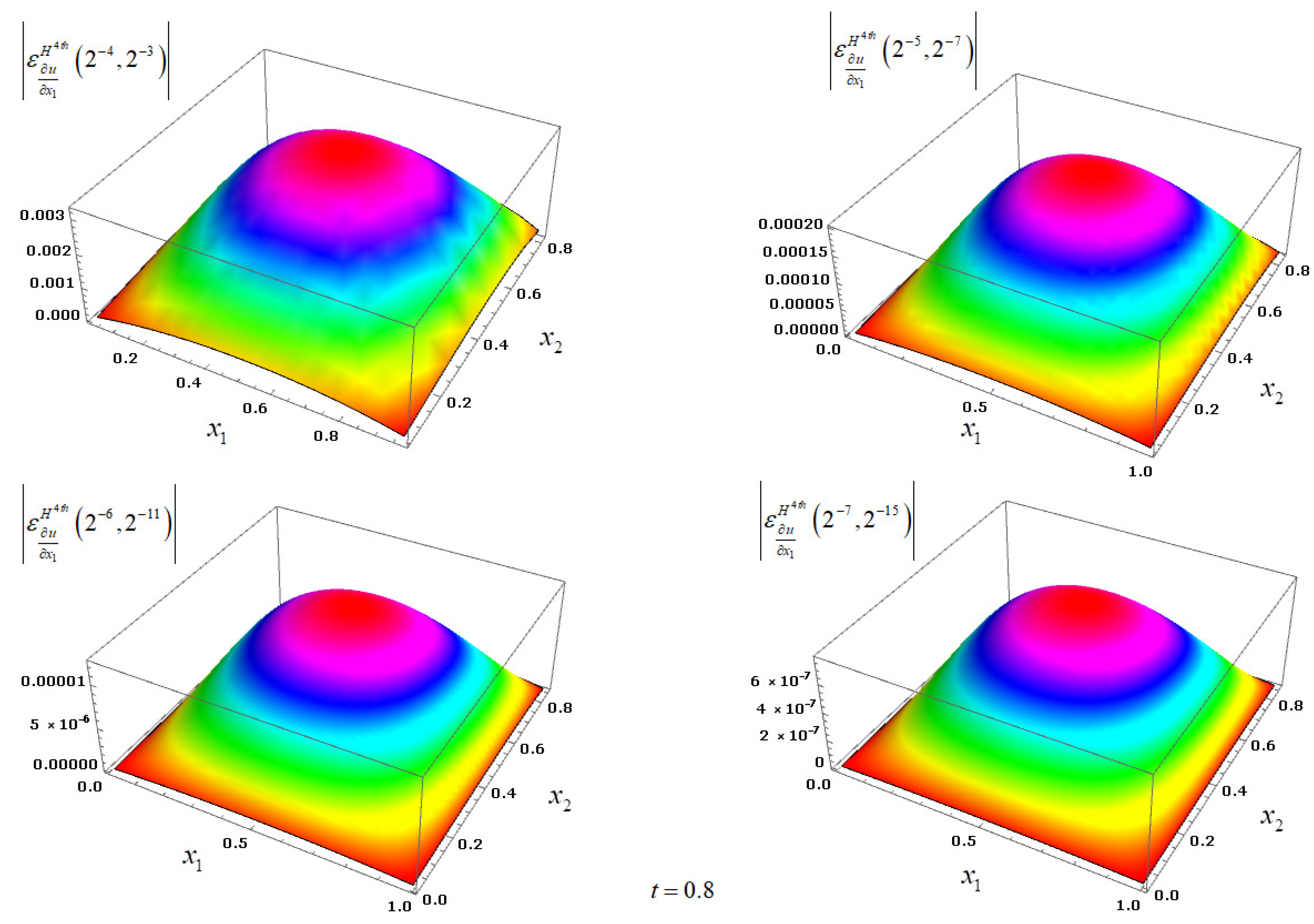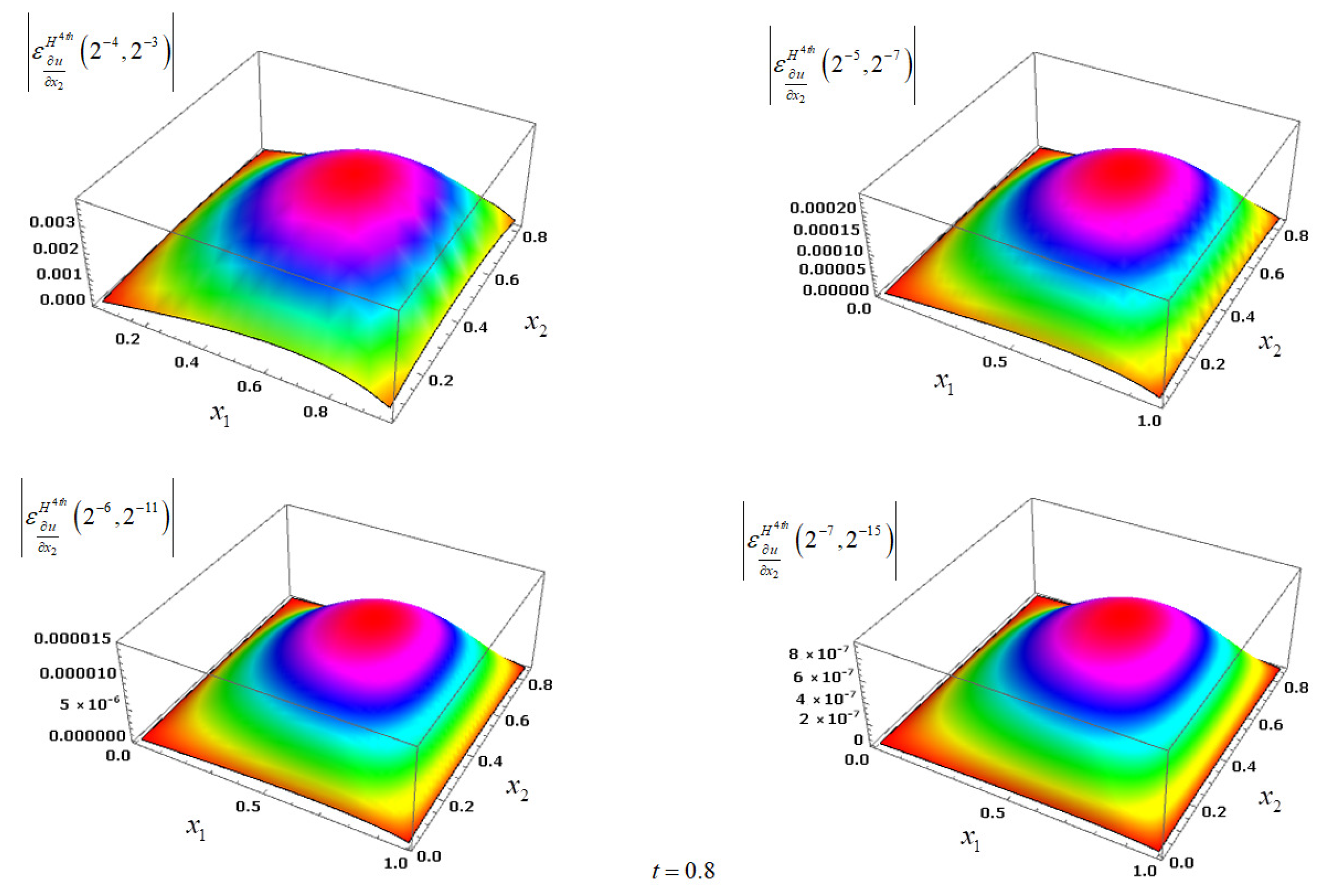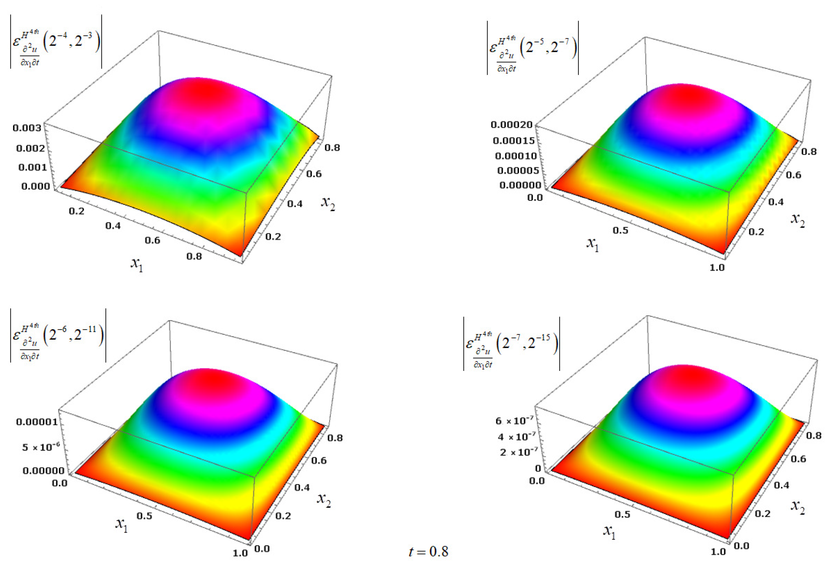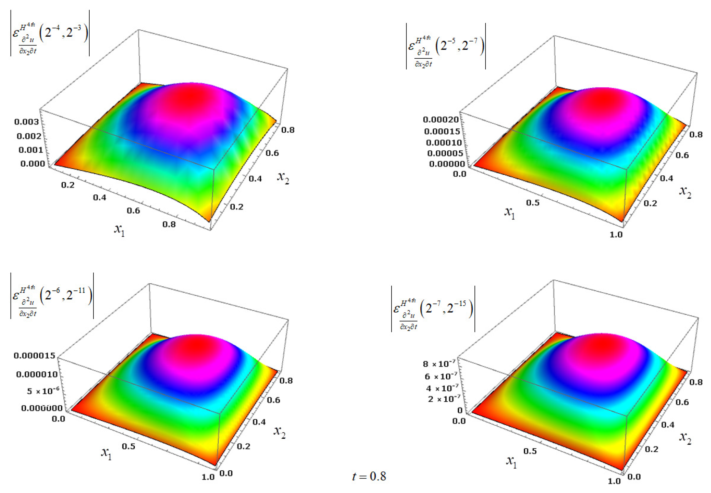Figure 4 and Figure 5 demonstrate the grid functions $\left|{\epsilon }_{\frac{{\partial }^{2}u}{\partial x_i\partial t}}^{H^{4th}}(2^{-4},2^{-3})\right|$, $\left|{\epsilon }_{\frac{{\partial }^{2}u}{\partial x_i\partial t}}^{H^{4th}}(2^{-5},2^{-7})\right|,$$\left|{\epsilon }_{\frac{{\partial }^{2}u}{\partial x_i\partial t}}^{H^{4th}}(2^{-6},2^{-11})\right|$ and $\left|{\epsilon }_{\frac{{\partial }^{2}u}{\partial x_i\partial t}}^{H^{4th}}(2^{-7},2^{-15})\right|$ for $i=1,2$ respectively, for $t=0.8$ achieved by applying the corresponding method $H^{4th}\left(\frac{{\partial }^{2}u}{\partial x_i\partial t}\right),$$i=1,2$ for the Example 1.

Figure 2. The grid function of absolute errors when $t=0.8$ obtained by the method $H^{4th}\left(\frac{\partial u}{\partial x_1}\right)$ for the Example 1.

Figure 3. The grid function of absolute errors when $t=0.8$ obtained by the method $H^{4th}\left(\frac{\partial u}{\partial x_2}\right)$ for the Example 1.

Figure 4. The grid function of absolute errors when $t=0.8$ obtained by the method $H^{4th}\left(\frac{{\partial }^{2}u}{\partial x_1\partial t}\right)$ for the Example 1.

Figure 5. The grid function of absolute errors when $t=0.8$ obtained by the method $H^{4th}\left(\frac{{\partial }^{2}u}{\partial x_2\partial t}\right)$ for the Example 1.

5.2. Test Problem Example 2

Equations are given as follows:

$$\begin{array}{ccc}\hfill \frac{\partial u}{\partial t}& =& 0.25\left(\frac{{\partial }^{2}u}{\partial x_1^2}+\frac{{\partial }^{2}u}{\partial x_2^2}\right)+f(x_1,x_2,t)\mathrm{on}{Q}_T,\hfill \\ \hfill u\left(x_1,x_2,0\right)& =& 0.01x_1{x}_2\left(1-x_1\right)\left(\frac{\sqrt{3}}{2}-x_2\right)\mathrm{on}\overline{D},\hfill \\ \hfill u\left(x_1,x_2,t\right)& =& 0\mathrm{on}{S}_T.\hfill \end{array}$$

The heat source function is

$$\begin{array}{ccc}\hfill f(x_1,x_2,t)& =& -0.01x_1{x}_2\left(1-x_1\right)\left(\frac{\sqrt{3}}{2}-x_2\right)sint\hfill \\ & & +0.005\left(x_1\left(1-x_1\right)+x_2\left(\frac{\sqrt{3}}{2}-x_2\right)\right)cost.\hfill \end{array}$$

The problem in Example 2 is a benchmark problem such that the solution is not provided. An analogous problem with zero heat source was also considered in Henner et al. [39]. By applying the proposed methods $H^{4th}\left(\frac{\partial u}{\partial x_i}\right),i=1,2,$ we obtain the approximate solutions $v_{2^{-\mu ,},2^{-\lambda }}$ and $z_{2^{-\mu ,},2^{-\lambda }}$ accordingly at every time level for the considered values $\mu =5,6$,7 and $\lambda =7,11,15$. Table 4 and Table 5 present $v_{2^{-\mu ,},2^{-\lambda }}\left(x_1,x_2,t\right)$ and $z_{2^{-\mu ,},2^{-\lambda }}\left(x_1,x_2,t\right)$, respectively, at the grid points $\left(0.125,\frac{\sqrt{3}}{8},1\right),$$\left(0.25,\frac{\sqrt{3}}{8},1\right),$$\left(0.375,\frac{\sqrt{3}}{8},1\right),$$\left(0.5,\frac{\sqrt{3}}{8},1\right),$$\left(0.625,\frac{\sqrt{3}}{8},1\right),$$\left(0.75,\frac{\sqrt{3}}{8},1\right)$ and $\left(0.875,\frac{\sqrt{3}}{8},1\right)$ and the corresponding order of convergence ${\Re }_{\frac{\partial u}{\partial x_i}}^{H^{4th}}\left(P\right)$ for $i=1,2$ at the grid point $P\left(x_1,x_2,t\right)$ given as

$$\begin{array}{ccc}\hfill {\Re }_{\frac{\partial u}{\partial x_1}}^{H^{4th}}\left(P\right)& =& \left|\frac{v_{2^{-5},2^{-7}}\left(P\right)-v_{2^{-6},2^{-11}}\left(P\right)}{v_{2^{-6},2^{-11}}\left(P\right)-v_{2^{-7},2^{-15}}\left(P\right)}\right|,\hfill \end{array}$$

(163)

$$\begin{array}{ccc}\hfill {\Re }_{\frac{\partial u}{\partial x_2}}^{H^{4th}}\left(P\right)& =& \left|\frac{z_{2^{-5},2^{-7}}\left(P\right)-z_{2^{-6},2^{-11}}\left(P\right)}{z_{2^{-6},2^{-11}}\left(P\right)-z_{2^{-7},2^{-15}}\left(P\right)}\right|.\hfill \end{array}$$

(164)

Table 4. The numerical solution $v_{h,\tau }$ at seven points when $t=1$, and the convergence orders obtained by $H^{4th}\left(\frac{\partial u}{\partial x_1}\right)$ for the Example 2.

P	${\mathit{v}}_{2^{-5},2^{-7}}\left(\mathit{P}\right)$	${\mathit{v}}_{2^{-6},2^{-11}}\left(\mathit{P}\right)$	${\mathit{v}}_{2^{-7},2^{-15}}\left(\mathit{P}\right)$	${\mathit{\Re }}_{\frac{\mathit{\partial }\mathit{u}}{\mathit{\partial }{\mathit{x}}_1}}^{{\mathit{H}}^{4\mathbf{th}}}\left(\mathit{P}\right)$
$\left(0.125,\frac{\sqrt{3}}{8},1\right)$	$0.000569713036$	$0.000569841548$	$0.000569849555$	$16.052$
$\left(0.25,\frac{\sqrt{3}}{8},1\right)$	$0.000379748416$	$0.000379890609$	$0.000379899468$	$16.049$
$\left(0.375,\frac{\sqrt{3}}{8},1\right)$	$0.000189857076$	$0.000189944236$	$0.000189949667$	$16.048$
$\left(0.5,\frac{\sqrt{3}}{8},1\right)$	$5.22\times {10}^{-16}$	$-3.27\times {10}^{-17}$	$1.87\times {10}^{-18}$	$16.046$
$\left(0.625,\frac{\sqrt{3}}{8},1\right)$	$-0.000189857076$	$-0.000189944236$	$-0.000189949667$	$16.048$
$\left(0.75,\frac{\sqrt{3}}{8},1\right)$	$-0.000379748416$	$-0.000379890609$	$-0.000379899468$	$16.049$
$\left(0.875,\frac{\sqrt{3}}{8},1\right)$	$-0.000569713036$	$-0.000569841548$	$-0.00056984955$	$16.052$

Table 5. The numerical solution $z_{h,\tau }$ at seven points when $t=1$, and the convergence orders obtained by $H^{4th}\left(\frac{\partial u}{\partial x_2}\right)$ for the Example 2.

P	${\mathit{z}}_{2^{-5},2^{-7}}\left(\mathit{P}\right)$	${\mathit{z}}_{2^{-6},2^{-11}}\left(\mathit{P}\right)$	${\mathit{z}}_{2^{-7},2^{-15}}\left(\mathit{P}\right)$	${\mathit{\Re }}_{\frac{\mathit{\partial }\mathit{u}}{\mathit{\partial }{\mathit{x}}_2}}^{{\mathit{H}}^{4\mathbf{th}}}\left(\mathit{P}\right)$
$\left(0.125,\frac{\sqrt{3}}{8},1\right)$	$0.000255810101$	$0.000255886243$	$0.000255890985$	$16.052$
$\left(0.25,\frac{\sqrt{3}}{8},1\right)$	$0.000438524584$	$0.000438661691$	$0.000438670233$	$16.052$
$\left(0.375,\frac{\sqrt{3}}{8},1\right)$	$0.000548151240$	$0.000548326834$	$0.000548337774$	$16.052$
$\left(0.5,\frac{\sqrt{3}}{8},1\right)$	$0.000584693185$	$0.000584881865$	$0.000584893620$	$16.052$
$\left(0.625,\frac{\sqrt{3}}{8},1\right)$	$0.000548151240$	$0.000548326834$	$0.000548337774$	$16.052$
$\left(0.75,\frac{\sqrt{3}}{8},1\right)$	$0.000438524584$	$0.000438661691$	$0.000438670233$	$16.052$
$\left(0.875,\frac{\sqrt{3}}{8},1\right)$	$0.000255810101$	$0.000255886242$	$0.000255890985$	$16.052$

By the same way Table 6 and Table 7 show $v_{t,2^{-\mu ,},2^{-\lambda }}\left(x_1,x_2,t\right)$ and $z_{t,2^{-\mu ,},2^{-\lambda }}\left(x_1,x_2,t\right)$, respectively, at the the considered grids and the corresponding convergence orders ${\Re }_{\frac{{\partial }^{2}u}{\partial x_i\partial t}}^{H^{4th}}\left(P\right)$ for $i=1,2$ at the point $P\left(x_1,x_2,t\right)$ defined as

$$\begin{array}{ccc}\hfill {\Re }_{\frac{{\partial }^{2}u}{\partial x_1\partial t}}^{H^{4th}}\left(P\right)& =& \left|\frac{v_{t,2^{-5},2^{-7}}\left(P\right)-v_{t,2^{-6},2^{-11}}\left(P\right)}{v_{t,2^{-6},2^{-11}}\left(P\right)-v_{t,2^{-7},2^{-15}}\left(P\right)}\right|,\hfill \end{array}$$

(165)

$$\begin{array}{ccc}\hfill {\Re }_{\frac{{\partial }^{2}u}{\partial x_2\partial t}}^{H^{4th}}\left(P\right)& =& \left|\frac{z_{t,2^{-5},2^{-7}}\left(P\right)-z_{t,2^{-6},2^{-11}}\left(P\right)}{z_{t,2^{-6},2^{-11}}\left(P\right)-z_{t,2^{-7},2^{-15}}\left(P\right)}\right|.\hfill \end{array}$$

(166)

Table 6. The numerical solution $v_{t,h,\tau }$ at seven points when $t=1$, and the convergence orders obtained by $H^{4th}\left(\frac{{\partial }^{2}u}{\partial x_1\partial t}\right)$ for the Example 2.

P	${\mathit{v}}_{\mathit{t},2^{-5},2^{-7}}\left(\mathit{P}\right)$	${\mathit{v}}_{\mathit{t},2^{-6},2^{-11}}\left(\mathit{P}\right)$	${\mathit{v}}_{\mathit{t},2^{-7},2^{-15}}\left(\mathit{P}\right)$	${\mathit{\Re }}_{\frac{{\mathit{\partial }}^2\mathit{u}}{\mathit{\partial }{\mathit{x}}_1\mathit{\partial }\mathit{t}}}^{{\mathit{H}}^{4\mathbf{th}}}\left(\mathit{P}\right)$
$\left(0.125,\frac{\sqrt{3}}{8},1\right)$	$-0.000887304144$	$-0.000887477357$	$-0.000887488206$	$15.966$
$\left(0.25,\frac{\sqrt{3}}{8},1\right)$	$-0.000591460365$	$-0.000591646827$	$-0.000591658507$	$15.964$
$\left(0.375,\frac{\sqrt{3}}{8},1\right)$	$-0.000295709687$	$-0.000295822129$	$-0.000295829173$	$15.963$
$\left(0.5,\frac{\sqrt{3}}{8},1\right)$	$7.22\times {10}^{-18}$	$3.33\times {10}^{-19}$	$-9.86\times {10}^{-20}$	$15.957$
$\left(0.625,\frac{\sqrt{3}}{8},1\right)$	$0.0002957096868$	$0.000295822129$	$0.000295829173$	$15.963$
$\left(0.75,\frac{\sqrt{3}}{8},1\right)$	$0.0005914603655$	$0.000591646827$	$0.000591658507$	$15.964$
$\left(0.875,\frac{\sqrt{3}}{8},1\right)$	$0.0008873041426$	$0.000887477357$	$0.000887488206$	$15.966$

Table 7. The numerical solution $z_{t,h,\tau }$ at seven points when $t=1$, and the convergence orders obtained by $H^{4th}\left(\frac{{\partial }^{2}u}{\partial x_2\partial t}\right)$ for the Example 2.

P	${\mathit{z}}_{\mathit{t},2^{-5},2^{-7}}\left(\mathit{P}\right)$	${\mathit{z}}_{\mathit{t},2^{-6},2^{-11}}\left(\mathit{P}\right)$	${\mathit{z}}_{\mathit{t},2^{-7},2^{-15}}\left(\mathit{P}\right)$	${\mathit{\Re }}_{\frac{{\mathit{\partial }}^2\mathit{u}}{\mathit{\partial }{\mathit{x}}_2\mathit{\partial }\mathit{t}}}^{{\mathit{H}}^{4\mathbf{th}}}\left(\mathit{P}\right)$
$\left(0.125,\frac{\sqrt{3}}{8},1\right)$	$-0.000398417531$	$-0.000398520228$	$-0.000398526661$	$15.966$
$\left(0.25,\frac{\sqrt{3}}{8},1\right)$	$-0.000682992442$	$-0.000683176968$	$-0.000683188526$	$15.966$
$\left(0.375,\frac{\sqrt{3}}{8},1\right)$	$-0.000853734894$	$-0.000853970855$	$-0.000853985635$	$15.965$
$\left(0.5,\frac{\sqrt{3}}{8},1\right)$	$-0.000910648720$	$-0.0009109021308$	$-0.000910918003$	$15.966$
$\left(0.625,\frac{\sqrt{3}}{8},1\right)$	$-0.000853734894$	$-0.0008539708553$	$-0.000853985635$	$15.966$
$\left(0.75,\frac{\sqrt{3}}{8},1\right)$	$-0.000682992442$	$-0.000683176968$	$-0.000683188526$	$15.965$
$\left(0.875,\frac{\sqrt{3}}{8},1\right)$	$-0.000398417531$	$-0.000398520228$	$-0.000398526661$	$15.966$

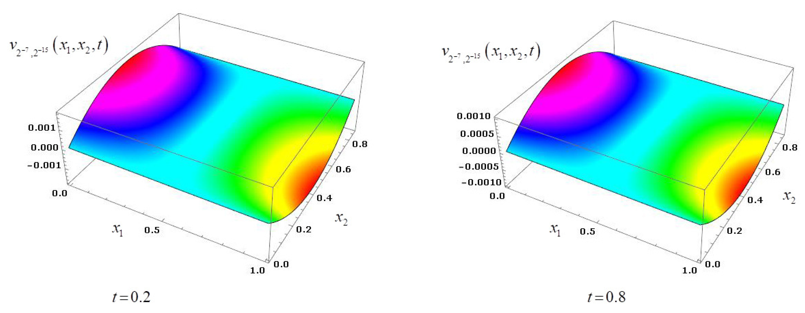
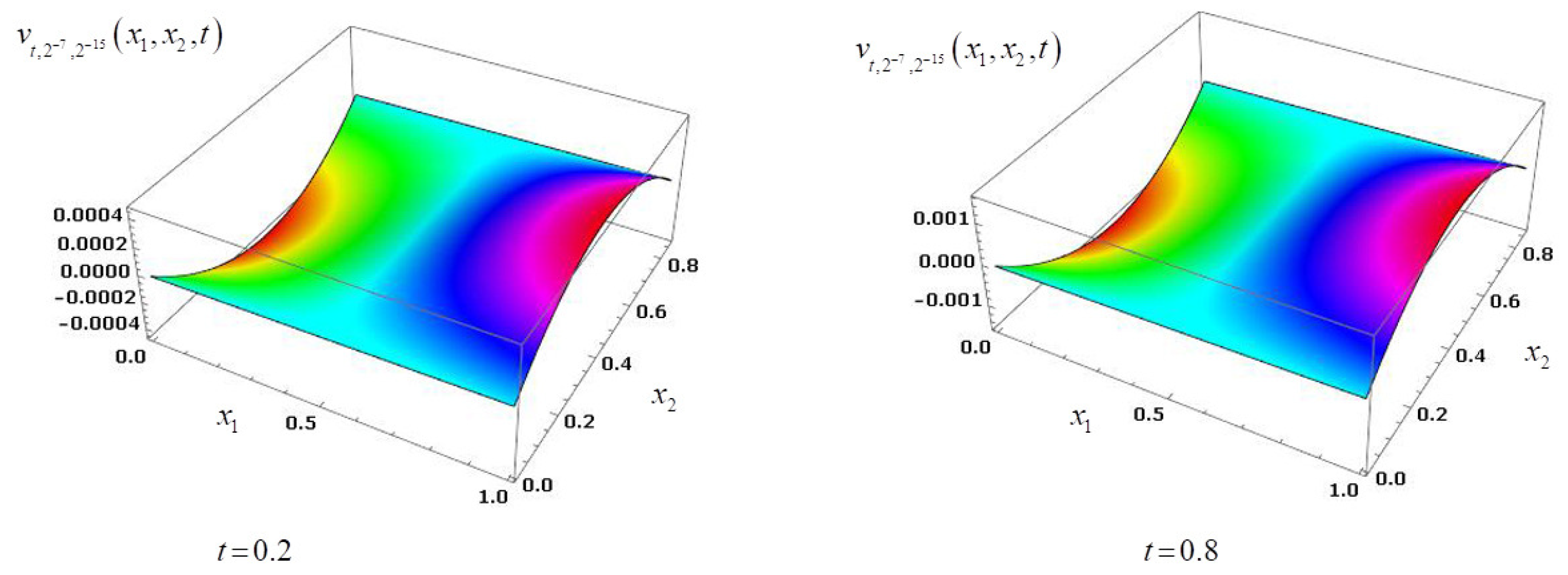
The computed solutions $v_{2^{-7},2^{-15}}$ and $z_{2^{-7},2^{-15}}$ achieved by using the corresponding two stage method $H^{4th}\left(\frac{\partial u}{\partial x_i}\right),i=1,2$ are demonstrated in Figure 6 and Figure 7 for the time levels $t=0.2$ and $t=0.8$. Figure 8 and Figure 9 illustrate the approximate solutions $v_{t,2^{-7},2^{-15}}$ and $z_{t,2^{-7},2^{-15}}$ taken by using the respective two stage method $H^{4th}\left(\frac{{\partial }^{2}u}{\partial x_1\partial t}\right),$$i=1,2$ for time levels $t=0.2$ and $t=0.8$.

Figure 6. The approximate solution $v_{2^{-7},2^{-15}}$ at time levels $t=0.2$ and $t=0.8$ obtained by the method $H^{4th}\left(\frac{\partial u}{\partial x_1}\right)$ for the Example 2.

Figure 7. The approximate solution $z_{2^{-7},2^{-15}}$ at time levels $t=0.2$ and $t=0.8$ obtained by the method $H^{4th}\left(\frac{\partial u}{\partial x_2}\right)$ for the Example 2.

Figure 8. The approximate solution $v_{t,2^{-7},2^{-15}}$ at time levels $t=0.2$ and $t=0.8$ obtained by the method $H^{4th}\left(\frac{{\partial }^{2}u}{\partial x_1\partial t}\right)$ for the Example 2.

Figure 9. The approximate solution $z_{t,2^{-7},2^{-15}}$ at time levels $t=0.2$ and $t=0.8$ obtained by the method $H^{4th}\left(\frac{{\partial }^{2}u}{\partial x_2\partial t}\right)$ for the Example 2.

6. Conclusions

Numerical methods using implicit schemes defined on hexagonal grids are proposed for computing the derivatives of the solution to Dirichlet problem of heat equation on rectangle. For the required smoothness conditions of the solution and when $r=\frac{\omega \tau }{h^2}\ge \frac{1}{16}$ the uniform convergence of the constructed difference schemes on the grids to the respective exact derivatives $\frac{\partial u}{\partial x_i}$ and $\frac{{\partial }^{2}u}{\partial x_i\partial t},i=1,2$ is shown to be $O\left(h^4+\tau \right)$.

Novelty Statement:

In Buranay et al. [26], we gave a second-order hexagonal grid approximation of the first-order spatial derivatives of the solution to BVP$\left(u\right)$ in (11) with the smoothness condition $u\in C_{x,t}^{7+\alpha ,\frac{7+\alpha }{2}},$$0<\alpha <1$ in the Hölder space. The method was established in two stages. In this study, we require that $u\in C_{x,t}^{9+\alpha ,\frac{9+\alpha }{2}}$, and give hexagonal grid computation of all the first order derivatives and the mixed order second order derivatives involving the time derivative by developing two stage implicit methods of fourth order accurate in space variables.