Guaranteed Cost Leaderless Consensus Protocol Design for Fractional-Order Uncertain Multi-Agent Systems with State and Input Delays

Abstract

This paper addresses the guaranteed cost leaderless consensus of delayed fractional-order (FO) multi-agent systems (FOMASs) with nonlinearities and uncertainties. A guaranteed cost function for FOMAS is proposed to simultaneously consider consensus performance and energy consumption. By employing the linear matrix inequality approach and the FO Razumikhin theorem, a delay-dependent and order-dependent consensus protocol is formulated for FOMASs with input delay. The proposed protocol not only guarantees the robust stability of the closed-loop system error but also ensures that the performance degradation caused by the system uncertainty is lesser than that obtained with other approaches. Two numerical examples are provided in order to verify the effectiveness and accuracy of the proposed protocol.

1. Introduction

In recent years, there has been increasing interest in the coordination of multi-agent systems (MASs) that have a variety of applications. For example, we can mention the distributed consensus behavior in sensor networks [1], satellite formation flying [2] and cooperative control of unmanned aerial vehicles rendezvous [3]. Consensus, as a critical dynamic behaviour in MASs, has been focused on integer-order (IO) MASs, where every agent is described by classical IO dynamics [4,5,6,7,8]. It has been shown that many phenomena can be explained naturally by coordinated behavior of agents with FO dynamics [9,10,11]. This includes flocking movement and food searching by means of individual secretions and microbial secretions, submarine underwater robots exploring seawater with a large number of microorganisms and viscous substances and operating unmanned aerial vehicles in complex space environments. Therefore, the question of how to achieve consensus for FOMASs has received much attention, and important developments involving leader-following group, cluster, finite-time, bipartite, group multiple lag and others have been presented. For example, nonlinear FOMASs with distributed input delays were considered in [12], a delay-dependent consensus condition for a class of linear FOMASs with distributed control containing input time-delay was proposed in [13], the event-triggered consensus for general linear FOMASs was investigated in [14,15] and the consensus of FOMASs without delay terms was studied in [16,17].

In practical applications, control systems are subject to time delays caused by the limited speed at which signals propagate [18]. Time delays may degrade system performance and robustness and even cause instability. Generally, consensus conditions of delayed FOMASs are divided into the categories of delay dependent and delay independent based on whether the consensus criteria depend on the delay or not. Usually, delay independent criteria are excessively conservative in comparison with delay dependent ones, particularly when the time delay is small. On the other hand, despite actual physical systems being nonlinear, there are few stability results for nonlinear delayed FOMASs. Therefore, addressing such systems is fundamental [19,20,21,22].

It should be mentioned that all works mentioned above focus only on the consensus regulation performance for FOMASs with the existence of time delays or/and nonlinearities [12,13,14,15,16,17,19,20,21,22]. However, energy consumption is an issue, and the so-called guaranteed cost control approach to tackle this problem, which considers the consensus regulation performance and the energy consumption at the same time, was proposed. The guaranteed cost consensus of MASs has increasingly attracted the attention of researchers. In [23], the event-triggered guaranteed cost consensus for nonlinear MASs with time delay and uncertain parameters was addressed. In [24], the guaranteed performance consensus for MASs with Lipschitz nonlinear dynamics was investigated. In [25,26], the guaranteed cost consensus for MASs was also investigated. However, it should be pointed out that most research has been focused on IO MASs instead of FOMASs and, in particular, the guaranteed cost consensus of FOMASs with state and input time-delay receiveed limited attention.

Motivated by the above discussion, a guaranteed cost leaderless consensus protocol for uncertain nonlinear delayed FOMASs with input time delay is proposed in this paper. The main contributions are the following: (1) to address the guaranteed cost consensus for nonlinear FOMASs with state and input time delay; (2) to establish in terms of linear matrix inequality (LMI) a delay-dependent and order-dependent sufficient condition for guaranteed cost leaderless consensus protocol; and (3) to obtain a guaranteed cost leaderless consensus protocol less conservative than the ones already proposed in the literature.

The rest of this paper is organized as follows. Section 2 introduces some fundamental concepts and lemmas necessary for theoretical development. Section 3 presents the main results and discusses the most relevant details. Section 4 demonstrates the effectiveness of the novel procedure with two numerical examples. Finally, Section 5 outlines the main conclusions.

Standard notation is used in the sequel. The symbols $R^{n*m}$, $\parallel *\parallel$ and ⊗ represent the set of real matrices, the Euclidean norm of a vector or the derived two-norm of a matrix and the Kronecker product, respectively. The symbol $I_N$ is an identity matrix, and diag{ * } denotes the diagonal matrix. The expression A > 0(≥0) represents a symmetric positive definite (semi-definite) matrix. The matrices $A^T$ and $A^{-1}$ denote the transpose and inverse of A, respectively.

2. Preliminaries and Problem Formulation

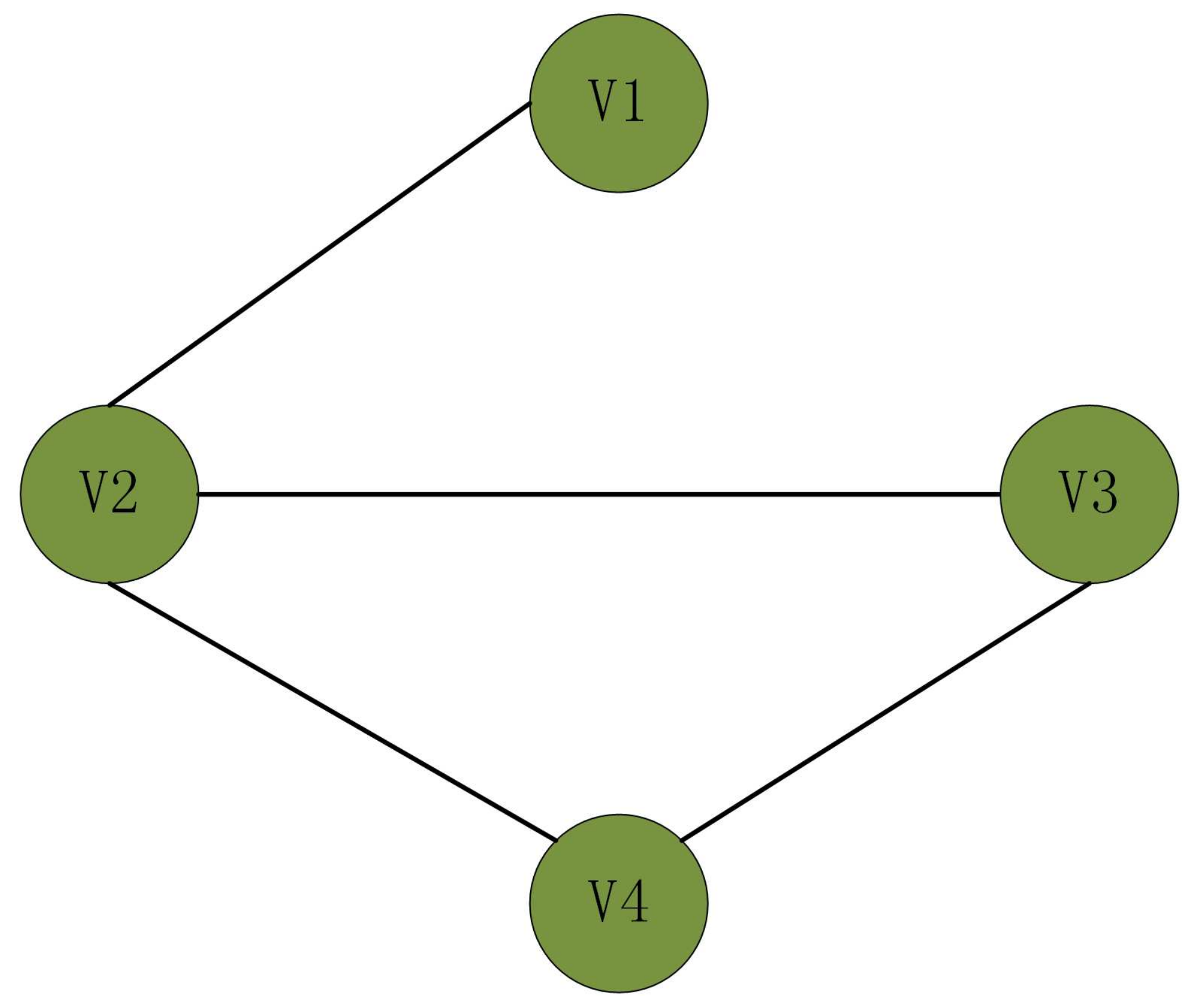
In this section, we introduce basic concepts of graph theory, definitions related to fractional calculus, guaranteed cost function related to FOMASs and some useful lemmas.

2.1. Graph Theory

An undirected graph G is a tuple $(V,E)$ in which $V=\{v_1,v_2,\cdots ,v_N\}$ denotes the set of nodes, and $E\subseteq V\times V$ is the set of edges of G. Any edge connecting nodes $v_i$ and $v_j$ is represented by $e_{ij}=(v_i,v_j)$ or $e_{ji}=(v_j,v_i)$ since we have $e_{ij}\in E\iff e_{ji}\in E$. For example, the tuple $(V,E)$ with $V=\{v_1,v_2,v_3,v_4\}$ and $E=\{(v_1,v_2),(v_2,v_2),(v_2,v_3),(v_1,v_3),(v_3,v_4)\}$, represents an undirected graph with four nodes and five edges. The number of edges associated with a node $v_i$ is called degree of the node, e.g., $deg\left(v_1\right)=2$ means that there are 2 edges associated with $v_1$. The adjacency matrix of the graph is $A={\left(a_{ij}\right)}_{N\times N}$, where $a_{ij}$ denotes the weight of edge $(i,j)$, the degree matrix corresponds to $D=diag\{d_1,d_2,\cdots ,d_N\}$ where the elements are defined by $d_i=\sum _j{a}_{ij}$ and the Laplacian of the weighted digraph G is defined as $L=D-A$, with each element in L expressed as follows.

$$\begin{array}{c}\hfill l_{ij}=\left\{\begin{array}{cc}& -a_{ij},i\ne j,\hfill \\ & {\Sigma }_{j=1,j\ne i}^N{a}_{ij},i=j.\hfill \end{array}\right.\end{array}$$

2.2. Useful Lemmas

Some useful lemmas are presented in the follow up.

Lemma 1.

All eigenvalues of $\tilde{L}$ are greater than or equal to 0 if and only if the graph G is connected, where the following is the case.

$$\begin{array}{c}\hfill \tilde{L}=\left[\begin{array}{cccc}{d}_2+a_{12}& a_{13}-a_{23}& \cdots & a_{1N}-a_{2N}\\ a_{12}-a_{32}& d_3+a_{13}& \cdots & a_{1N}-a_{3N}\\ ⋮& ⋮& ⋮& ⋮\\ a_{12}-a_{N2}& a_{13}-a_{N3}& \cdots & d_N+a_{1N}\end{array}\right].\end{array}$$

Proof. 

Let $1_{n-1}^T=\underset{n-1}{\underbrace{[1,\cdots ,1]}}$, $0_{N-1}=\underset{n-1}{\underbrace{[0,\cdots ,0]}}$ and the following be the case:

$$\begin{array}{c}\hfill Q=\left[\begin{array}{cc}1& 0_{N-1}\\ -1_{n-1}& I_{n-1}\end{array}\right],\end{array}$$

where $I_{n-1}$ is an identity matrix with dimension $n-1$. Then, we have the following:

$$\begin{array}{c}\hfill QL{Q}^{-1}=\left[\begin{array}{cc}0& a\\ 0_{n-1}^T& \tilde{L}\end{array}\right],\end{array}$$

where $a=[-a_{12},\cdots ,-a_{1n}]$. Since all eigenvalues of matrix L are greater than or equal to 0 if and only if G is connected, then Lemma 1 holds. □

Lemma 2.

The Laplacian L of the undirected graph obeys the following [27]:

$$\begin{array}{c}\hfill x^{\mathrm{T}}\left(t\right)Lx\left(t\right)=\frac{1}{2}\sum _{i=1}^N\sum _{j=1}^N{a}_{ij}{(x_i\left(t\right)-x_j\left(t\right))}^{\mathrm{T}}(x_i\left(t\right)-x_j\left(t\right)),\end{array}$$

and $L=L^{\mathrm{T}}\ge 0$.

Lemma 3.

For given matrices $Q=Q^{\mathrm{T}}$, H, M and $R=R^{\mathrm{T}}$ with appropriate dimensions [28], the following condition:

$$\begin{array}{c}\hfill Q+HNM+M^{\mathrm{T}}{N}^{\mathrm{T}}{H}^{\mathrm{T}}<0\end{array}$$

is verified for $N\left(t\right)N^{\mathrm{T}}\left(t\right)\le R$ if and only if there exists some $\lambda >0$ such that the following is the case.

$$\begin{array}{c}\hfill Q+\lambda H{H}^{\mathrm{T}}+{\lambda }^{-1}{M}^{\mathrm{T}}RM<0.\end{array}$$

Lemma 4.

When $x\left(t\right)\in R^n$ is a differentiable vector-value function, $P=P^{\mathrm{T}}>0$ and $\forall \alpha \in (0,1)$ [29]. We can obtain the following.

$$\begin{array}{c}\hfill {}_{t_0}^C{D}_t^{\alpha }(x^{\mathrm{T}}\left(t\right)Px\left(t\right)\le {\left(x^{\mathrm{T}}\left(t\right)P\right)}_{t_0}^C{D}_t^{\alpha }x\left(t\right)+{{(}_{t_0}^C{D}_t^{\alpha }x\left(t\right))}^{\mathrm{T}}Px\left(t\right).\end{array}$$

Lemma 5.

For any real vectors with the same dimension x and y, the following inequality is verified [30]:

$$\begin{array}{c}\hfill 2x^{T}y\le \epsilon x^{T}x+{\epsilon }^{-1}{y}^{T}y,\end{array}$$

where ε is a positive number.

2.3. Problem Statement

The i-th agent can be modeled as follows:

$$\begin{array}{c}\hfill {}_{t_0}^C{D}_t^{\alpha }{x}_i\left(t\right)=(A+\mathrm{\Delta }A)x_i\left(t\right)+(A_{\tau }+\mathrm{\Delta }{A}_{\tau })x_i(t-\tau )+f\left(x_i\left(t\right)\right)+(B+\mathrm{\Delta }B)u_i\left(t\right),i=1,2\cdots N,\end{array}$$

(1)

where $x_i\left(t\right)={[x_{i1}\left(t\right),x_{i2}\left(t\right)\cdots x_{in}\left(t\right)]}^{\mathrm{T}}$, ${}_{t_0}^C{D}_t^{\alpha }x\left(t\right)=\frac{1}{\mathrm{\Gamma }(n-\alpha )}{\int }_{t_0}^t\frac{x^n\left(s\right)}{{(t-s)}^{\alpha -n+1}}ds$, and $\mathrm{\Gamma }\left(s\right)={\int }_0^{\infty }{t}^{s-1}{e}^{-t}dt$ is the Gamma function. The variable $u_i\left(t\right)$ represents the control input and A, and $A_{\tau }\in R^{n\times n}$ and $B\in R^{n\times m}$ are known constant matrices. The symbols $\mathrm{\Delta }A$, $\mathrm{\Delta }{A}_{\tau }$ and $\mathrm{\Delta }B$ represent uncertain matrices given by the following:

$$\left[\hspace{1em}\mathrm{\Delta }A\hspace{1em}\mathrm{\Delta }{A}_{\tau }\hspace{1em}\mathrm{\Delta }B\hspace{1em}\right] = EH\left(t\right) \left[\hspace{1em}{F}_1\hspace{1em}{F}_2\hspace{1em}{F}_3\hspace{1em}\right],$$

where E, $F_1$, $F_2$ and $F_3$ are known constant real matrices with appropriate dimensions, and $H\left(t\right)$ is the unknown time-varying matrix satisfying $H\left(t\right)H^{\mathrm{T}}\left(t\right)\le I$. Moreover, $f:R^n\to R^n$ is a continuous function that satisfies the Lipschitz condition. There is a positive constant l such that the following is the case.

$$\begin{array}{c}\hfill \parallel f\left(x\right)-f\left(y\right)\parallel \le l\parallel x-y\parallel ,\forall x,y\in R^n.\end{array}$$

Remark 1.

If $f\left(x_i\left(t\right)\right)$= 0, then the model of the i-th agent can be expressed as follows.

$$\begin{array}{c}\hfill {}_{t_0}^C{D}_t^{\alpha }{x}_i\left(t\right)=(A+\mathrm{\Delta }A)x_i\left(t\right)+(A_{\tau }+\mathrm{\Delta }{A}_{\tau })x_i(t-\tau )+(B+\mathrm{\Delta }B)u_i\left(t\right),i=1,2\cdots N.\end{array}$$

(2)

The control protocol will be designed as follows:

$$\begin{array}{c}\hfill u_i\left(t\right)=-K\left(\sum _{j\in N_i}(a_{ij}(x_i(t-\tau )-x_j(t-\tau ))\right).\end{array}$$

(3)

where K is feedback control gain.

Definition 1.

The consensus of MASs without a leader can be achieved if and only if the following is the case [30].

$$\begin{array}{c}\hfill \underset{t\to \infty }{lim}\parallel x_i\left(t\right)-x_1\left(t\right)\parallel =0.\end{array}$$

Let $e_i\left(t\right)=x_i\left(t\right)-x_1\left(t\right)$. By Definition 1, if ${lim}_{t\to \infty }\parallel e_i\left(t\right)\parallel =0$, then consensus for system (1) can be achieved. It follows from system (1) and (2) that the following error systems can be obtained.

$$\begin{array}{cc}\hfill {}_{t_0}^C{D}_t^{\alpha }{e}_i\left(t\right)& =(A+\mathrm{\Delta }A)e_i\left(t\right)+(A_{\tau }+\mathrm{\Delta }{A}_{\tau })e_i(t-\tau )+(B+\mathrm{\Delta }B)u_i\left(t\right)-(B+\mathrm{\Delta }B)u_1\left(t\right)\hfill \\ & +f\left(x_i\left(t\right)\right)-f\left(x_1\left(t\right)\right),\hfill \end{array}$$

(4)

$$\begin{array}{ccc}\hfill {}_{t_0}^C{D}_t^{\alpha }{e}_i\left(t\right)& =& (A+\mathrm{\Delta }A)e_i\left(t\right)+(A_{\tau }+\mathrm{\Delta }{A}_{\tau })e_i(t-\tau )+(B+\mathrm{\Delta }B)u_i\left(t\right)-(B+\mathrm{\Delta }B)u_1\left(t\right).\hfill \end{array}$$

(5)

Definition 2.

The guaranteed cost function associated with FOMASs ($0\le \alpha \le 1$) is defined as follows:

$$\begin{array}{c}\hfill J=\frac{1}{\mathrm{\Gamma }\left(\alpha \right)}{\int }_0^t{(t-s)}^{\alpha -1}(J_x\left(s\right)+J_u\left(s\right))ds,\end{array}$$

(6)

where

$$\begin{array}{ccc}\hfill J_x\left(t\right)& =& \sum _{i=1}^N\sum _{j=1}^N{a}_{ij}{(x_i\left(t\right)-x_j\left(t\right))}^{\mathrm{T}}{Q}_1(x_i\left(t\right)-x_j\left(t\right)),\hfill \\ \hfill J_u\left(t\right)& =& \sum _{i=1}^N{u}_i^{\mathrm{T}}\left(t\right)Q_2{u}_i\left(t\right),\hfill \end{array}$$

with $Q_1$ and $Q_2$ representing two given symmetric positive matrices.

Remark 2.

In (6), $J_x\left(t\right)$ and $J_u\left(t\right)$ represent the consensus error performance and the control energy consumption for the FOMASs. Reference [31] addressed the guaranteed cost of control for a single system. The works [23,24,25,26,32,33] proposed a guaranteed cost function related to MASs, but that cannot be applied to the guaranteed cost consensus of FOMASs. Therefore, the definition of the guaranteed cost function (6) related to FOMASs is given.

3. Main Results

In this section, a delay-dependent sufficient condition for the guaranteed cost consensus protocol is established in terms of LMI, and its guaranteed cost is derived.

Theorem 1.

For given positive definite symmetric matrices $Q_1$ and $Q_2$, if there exist a symmetric positive definite matrix $\overline{P}$, a matrix Y and the constant positive scalars λ such that the following is the case:

$$\begin{array}{c}\hfill \mathrm{\Delta }=\left[\begin{array}{ccccccccc}{\mathrm{\Delta }}_{11}& {\mathrm{\Delta }}_{12}& {\mathrm{\Delta }}_{13}& {\mathrm{\Delta }}_{14}& {\mathrm{\Delta }}_{15}& {\mathrm{\Delta }}_{16}& {\mathrm{\Delta }}_{17}& {\mathrm{\Delta }}_{18}& 0\\ *& {\mathrm{\Delta }}_{22}& {\mathrm{\Delta }}_{23}& {\mathrm{\Delta }}_{24}& 0& 0& 0& 0& {\mathrm{\Delta }}_{29}\\ *& *& {\mathrm{\Delta }}_{33}& 0& {\mathrm{\Delta }}_{35}& 0& 0& 0& 0\\ *& *& *& {\mathrm{\Delta }}_{44}& 0& 0& 0& 0& 0\\ *& *& *& *& {\mathrm{\Delta }}_{55}& 0& 0& 0& 0\\ *& *& *& *& *& {\mathrm{\Delta }}_{66}& 0& 0& 0\\ *& *& *& *& *& *& {\mathrm{\Delta }}_{77}& 0& 0\\ *& *& *& *& *& *& *& {\mathrm{\Delta }}_{88}& 0\\ *& *& *& *& *& *& *& *& {\mathrm{\Delta }}_{99}\end{array}\right]<0,\end{array}$$

(7)

where

$$\begin{array}{ccc}\hfill {\mathrm{\Delta }}_{11}& =& I_{N-1}\otimes (\overline{P}{A}^{\mathrm{T}}+A\overline{P}+\overline{P}+I),\hfill \\ \hfill {\mathrm{\Delta }}_{12}& =& I_{N-1}\otimes A_{\tau }\overline{P}-\tilde{L}\otimes BY,\hfill \\ \hfill {\mathrm{\Delta }}_{13}& =& {\tau }^{\alpha }{\alpha }^{-1}{I}_{N-1}\otimes \overline{P}{A}^{\mathrm{T}},{\mathrm{\Delta }}_{14}=I_{N-1}\otimes \overline{P}{F}_1^{\mathrm{T}},\hfill \\ \hfill {\mathrm{\Delta }}_{15}& =& I_{N-1}\otimes \lambda E,{\mathrm{\Delta }}_{16}=I_{N-1}\otimes l^2\overline{P},\hfill \\ \hfill {\mathrm{\Delta }}_{17}& =& I_{N-1}\otimes {\tau }^{\alpha }{\alpha }^{-1}\overline{P},{\mathrm{\Delta }}_{18}=2{\lambda }_{max}\left(L\right)I_{N-1}\otimes \overline{P}{Q}_1,\hfill \\ \hfill {\mathrm{\Delta }}_{22}& =& -I_{N-1}\otimes \overline{P},\hfill \\ \hfill {\mathrm{\Delta }}_{23}& =& {\tau }^{\alpha }{\alpha }^{-1}(I_{N-1}\otimes \overline{P}{A}_{\tau }^{\mathrm{T}}-{\tilde{L}}^{\mathrm{T}}\otimes Y^{\mathrm{T}}{B}^{\mathrm{T}}),\hfill \\ \hfill {\mathrm{\Delta }}_{24}& =& I_{N-1}\otimes \overline{P}{F}_2^{\mathrm{T}}-{\tilde{L}}^{\mathrm{T}}\otimes Y^{\mathrm{T}}{F}_3^{\mathrm{T}},\hfill \\ \hfill {\mathrm{\Delta }}_{29}& =& {\lambda }_{max}^2\left(L\right)I_{N-1}\otimes Y^{\mathrm{T}}{Q}_2,\hfill \\ \hfill {\mathrm{\Delta }}_{33}& =& {\mathrm{\Omega }}_{77}=-I_{N-1}\otimes {\tau }^{\alpha }{\alpha }^{-1}I,{\mathrm{\Omega }}_{35}={\tau }^{\alpha }{\alpha }^{-1}{I}_{N-1}\otimes \lambda E,\hfill \\ \hfill {\mathrm{\Delta }}_{44}& =& {\mathrm{\Omega }}_{55}=-I_{N-1}\otimes \lambda I,{\mathrm{\Delta }}_{66}=-I_{N-1}\otimes l^{2}I,\hfill \\ \hfill {\mathrm{\Delta }}_{88}& =& -2{\lambda }_{max}\left(L\right)I_{N-1}\otimes Q_1,\hfill \\ \hfill {\mathrm{\Delta }}_{99}& =& -{\lambda }_{max}^2\left(L\right)I_{N-1}\otimes Q_2,\hfill \end{array}$$

then the consensus of the FOMASs (1) with control protocol (3) is achieved. Moreover, the feedback gain K is given by the following:

$$\begin{array}{c}\hfill K=Y{\overline{P}}^{-1},\end{array}$$

and the guaranteed cost defined as follows.

$$\begin{array}{c}\hfill J^{*}={\lambda }_{max}(I_{N-1}\otimes P){\parallel e\left(0\right)\parallel }^2.\end{array}$$

Proof. 

According to (3) and (5), one obtains the following:

$$\begin{array}{ccc}\hfill {}_{t_0}^C{D}_t^{\alpha }{e}_i\left(t\right)& =& (A+\mathrm{\Delta }A)e_i\left(t\right)+(A_{\tau }+\mathrm{\Delta }{A}_{\tau })e_i(t-\tau )-(B+\mathrm{\Delta }B)K(\sum _{j\in N_i}(a_{ij}(x_i(t-\tau )-x_j(t-\tau ))\hfill \\ & +& (B+\mathrm{\Delta }B)K(\sum _{j\in N_i}\left(a_{1j}(x_1(t-\tau )-x_j(t-\tau ))\right)+f\left(x_i\left(t\right)\right)-f\left(x_1\left(t\right)\right),\hfill \end{array}$$

which can be written as follows:

$$\begin{array}{c}\hfill {}_{t_0}^C{D}_t^{\alpha }e\left(t\right)=I_{N-1}\otimes (A+\mathrm{\Delta }A)e\left(t\right)+I_{N-1}\otimes (A_{\tau }+\mathrm{\Delta }{A}_{\tau })e(t-\tau )\\ \hfill -\tilde{L}\otimes (BK+\mathrm{\Delta }BK)e(t-\tau )+F\left(x\left(t\right)\right),\end{array}$$

where $e\left(t\right)={[e_2^T\left(t\right),\cdots ,e_n^T\left(t\right)]}^T$, $e(t-\tau )=[e_2^T(t-\tau ),\cdots ,e_n^T{\left((t-\tau )\right]}^T$ and $F\left(x\left(t\right)\right)={[{(f\left(x_2\left(t\right)\right)-f\left(x_1\left(t\right)\right))}^T,{(f\left(x_3\left(t\right)\right)-f\left(x_1\left(t\right)\right))}^T,\cdots ,{(f\left(x_N\left(t\right)\right)-f\left(x_1\left(t\right)\right))}^T]}^T$.

From the definition of guaranteed cost function, the following is the case:

$$\begin{array}{ccc}& & {\overline{e}}^{\mathrm{T}}\left(t\right)(2L\otimes Q_1)\overline{e}\left(t\right)+{\overline{e}}^{\mathrm{T}}(t-\tau )(L^{\mathrm{T}}L\otimes K^{\mathrm{T}}{Q}_{2}K)\overline{e}(t-\tau )\hfill \\ & \le & e^{\mathrm{T}}\left(t\right)(2{\lambda }_{max}\left(L\right)I_{N-1}\otimes Q_1)e\left(t\right)+e^{\mathrm{T}}(t-\tau )({\lambda }_{max}^2\left(L\right)I_{N-1}\otimes K^{\mathrm{T}}{Q}_{2}K)e(t-\tau ),\hfill \end{array}$$

where $\overline{e}\left(t\right)={[e_1^T\left(t\right),\cdots ,e_n^T\left(t\right)]}^T$ and $\overline{e}(t-\tau )=[e_1^T(t-\tau ),\cdots ,e_n^T{\left((t-\tau )\right]}^T$.

Let us select a Lyapunov function.

$$\begin{array}{c}\hfill V\left(t\right)=e^{\mathrm{T}}\left(t\right)(I_{N-1}\otimes P)e\left(t\right).\end{array}$$

Taking the $\alpha$-order derivative and using Lemma 4 results in the following.

$$\begin{array}{ccc}\hfill {}_{t_0}^C{D}_t^{\alpha }V\left(t\right)& +& e^{\mathrm{T}}\left(t\right)(2L\otimes Q_1)e\left(t\right)+e^{\mathrm{T}}\left(t\right)(L^{\mathrm{T}}L\otimes K^{\mathrm{T}}{Q}_{2}K)e\left(t\right)\hfill \\ & \le & e^{\mathrm{T}}\left(t\right){(I_{N-1}\otimes P)}_{t_0}^C{D}_t^{\alpha }e\left(t\right)+{{(}_{t_0}^C{D}_t^{\alpha }e\left(t\right))}^{\mathrm{T}}(I_{N-1}\otimes P)e\left(t\right)\hfill \\ & +& e^{\mathrm{T}}\left(t\right)(2L\otimes Q_1)e\left(t\right)+e^{\mathrm{T}}(t-\tau )({\tilde{L}}^{\mathrm{T}}\tilde{L}\otimes K^{\mathrm{T}}{Q}_{2}K)e(t-\tau )\hfill \\ & \le & e^{\mathrm{T}}\left(t\right)(I_{N-1}\otimes (A^{\mathrm{T}}P+PA+\mathrm{\Delta }{A}^{\mathrm{T}}P+P\mathrm{\Delta }A))e\left(t\right)\hfill \\ & +& e^{\mathrm{T}}(t-\tau )(I_{N-1}\otimes (A_{\tau }^{\mathrm{T}}P+\mathrm{\Delta }{A}_{\tau }^{\mathrm{T}}P)\hfill \\ & -& {\tilde{L}}^{\mathrm{T}}\otimes (K^{\mathrm{T}}{B}^{\mathrm{T}}P+K^{\mathrm{T}}\mathrm{\Delta }{B}^{\mathrm{T}}P))e\left(t\right)+e^{\mathrm{T}}\left(t\right)(I_{N-1}\otimes (P{A}_{\tau }+P\mathrm{\Delta }{A}_{\tau })\hfill \\ & -& \tilde{L}\otimes (PBK+P\mathrm{\Delta }BK))e(t-\tau )+e^{\mathrm{T}}\left(t\right)(2{\lambda }_{max}\left(L\right)I_{N-1}\otimes Q_1)e\left(t\right)\hfill \\ & +& e^{\mathrm{T}}(t-\tau )({\lambda }_{max}^2\left(L\right)I_{N-1}\otimes K^{\mathrm{T}}{Q}_{2}K)e(t-\tau )+e^{\mathrm{T}}\left(t\right)(I_{N-1}\otimes P)F\left(x\left(t\right)\right)\hfill \\ & +& F^{\mathrm{T}}\left(x\left(t\right)\right)(I_{N-1}\otimes P)e\left(t\right).\hfill \end{array}$$

(8)

It follows from Lemma 5 that there exist two positive constants $ϵ$ and $\epsilon$ such that the following is the case.

$$\begin{array}{ccc}\hfill e^{\mathrm{T}}\left(t\right)(I_{N-1}\otimes P)F\left(x\left(t\right)\right)& +& F^{\mathrm{T}}\left(x\left(t\right)\right)(I_N\otimes P)e\left(t\right)\hfill \\ & \le & e^{\mathrm{T}}\left(t\right)(\frac{1}{2}({ϵ}^{-1}+\epsilon )l^2{I}_{N-1}\otimes I\hfill \\ & +& \frac{1}{2}(ϵ+{\epsilon }^{-1})I_{N-1}\otimes P^2)e\left(t\right).\hfill \end{array}$$

For the analysis, let us consider $ϵ=\epsilon =1$. Then, one obtains the following:

$$\begin{array}{ccc}\hfill e^{\mathrm{T}}\left(t\right)(I_{N-1}\otimes P)F\left(x\left(t\right)\right)& +& F^{\mathrm{T}}\left(x\left(t\right)\right)(I_N\otimes P)e\left(t\right)\hfill \\ & \le & e^{\mathrm{T}}\left(t\right)(I_{N-1}\otimes l^{2}I+I_{N-1}\otimes P^2)e\left(t\right).\hfill \end{array}$$

(9)

while $-\tau \le \theta \le 0$, $e\left(t\right)$ satisfies the following.

$$\begin{array}{c}\hfill V(t+\theta ,e(t+\theta \left)\right)<\mu V(t,e(t\left)\right)\end{array}$$

When $\mu >1$, one can obtain the following.

$$\begin{array}{c}\hfill \mu e^{\mathrm{T}}\left(t\right)(I_{N-1}\otimes P)e\left(t\right)-e^{\mathrm{T}}(t-\tau )(I_{N-1}\otimes P)e(t-\tau )\ge 0.\end{array}$$

(10)

Combining $(8)$ with $(10)$ yields the following.

$$\begin{array}{ccc}\hfill {}_{t_0}^C{D}_t^{\alpha }V\left(t\right)& +& e^{\mathrm{T}}\left(t\right)(2{\lambda }_{max}\left(L\right)I_{N-1}\otimes Q_1)e\left(t\right)+e^{\mathrm{T}}(t-\tau )({\lambda }_{max}^2\left(L\right)I_{N-1}\otimes K^{\mathrm{T}}{Q}_{2}K)e(t-\tau )\hfill \\ & \le & e^{\mathrm{T}}\left(t\right)(I_{N-1}\otimes (A^{\mathrm{T}}P+PA+\mathrm{\Delta }{A}^{\mathrm{T}}P+P\mathrm{\Delta }A+l^{2}I\hfill \\ & +& P^2+\mu P+2{\lambda }_{max}\left(L\right)Q_1\left)\right)e\left(t\right)+e^{\mathrm{T}}(t-\tau )(I_{N-1}\otimes (A_{\tau }^{\mathrm{T}}P+\mathrm{\Delta }{A}_{\tau }^{\mathrm{T}}P)\hfill \\ & -& {\tilde{L}}^{\mathrm{T}}\otimes (K^{\mathrm{T}}{B}^{\mathrm{T}}P+K^{\mathrm{T}}\mathrm{\Delta }{B}^{\mathrm{T}}P))e\left(t\right)+e^{\mathrm{T}}\left(t\right)(I_{N-1}\otimes (P{A}_{\tau }+P\mathrm{\Delta }{A}_{\tau })\hfill \\ & -& \tilde{L}\otimes (PBK+P\mathrm{\Delta }BK))e(t-\tau )\hfill \\ & -& e^{\mathrm{T}}(t-\tau )(I_{N-1}\otimes P+{\lambda }_{max}^2\left(L\right)K^{\mathrm{T}}{Q}_{2}K)e(t-\tau ).\hfill \end{array}$$

(11)

Moreover, for symmetric real matrices $X=X^{\mathrm{T}}$, $Z=Z^{\mathrm{T}}$ and matrix W, we have the following.

$$\begin{array}{c}\hfill \mathrm{\Omega }=\left[\begin{array}{cc}X& W\\ W^{\mathrm{T}}& Z\end{array}\right]\ge 0.\end{array}$$

Then, the following inequality holds:

$$\begin{array}{c}\hfill {\tau }^{\alpha }{\alpha }^{-1}{\zeta }^{\mathrm{T}}\left(t\right)\mathrm{\Omega }\zeta \left(t\right)-{\int }_{t-\tau \left(t\right)}^t{(t-s)}^{\alpha -1}{\zeta }^{\mathrm{T}}\left(t\right)\mathrm{\Omega }\zeta \left(t\right)ds\ge 0,\end{array}$$

(12)

where $\zeta \left(t\right)={[e^{\mathrm{T}}\left(t\right),{{(}_{t_0}^C{D}_t^{\alpha }V\left(t\right))}^{\mathrm{T}}]}^{\mathrm{T}}$. Let $X=Z=I_{N-1}\otimes I_n,W=0_{(N-1)n}$ for simplicity. According to $(11)$ and $(12)$, one obtains the following:

$$\begin{array}{ccc}\hfill {}_{t_0}^C{D}_t^{\alpha }V\left(t\right)& +& e^{\mathrm{T}}\left(t\right)(2{\lambda }_{max}\left(L\right)I_{N-1}\otimes Q_1)e\left(t\right)+e^{\mathrm{T}}(t-\tau )({\lambda }_{max}^2\left(L\right)I_{N-1}\otimes K^{\mathrm{T}}{Q}_{2}K)e(t-\tau )\hfill \\ & \le & e^{\mathrm{T}}\left(t\right)(I_{N-1}\otimes (A^{\mathrm{T}}P+PA+\mathrm{\Delta }{A}^{\mathrm{T}}P+P\mathrm{\Delta }A+l^{2}I\hfill \\ & +& P^2+\mu P+2{\lambda }_{max}\left(L\right)Q_1\left)\right)e\left(t\right)+e^{\mathrm{T}}(t-\tau )(I_{N-1}\otimes (A_{\tau }^{\mathrm{T}}P+\mathrm{\Delta }{A}_{\tau }^{\mathrm{T}}P)\hfill \\ & -& {\tilde{L}}^{\mathrm{T}}\otimes (K^{\mathrm{T}}{B}^{\mathrm{T}}P+K^{\mathrm{T}}\mathrm{\Delta }{B}^{\mathrm{T}}P))e\left(t\right)+e^{\mathrm{T}}\left(t\right)(I_{N-1}\otimes (P{A}_{\tau }+P\mathrm{\Delta }{A}_{\tau })\hfill \\ & -& \tilde{L}\otimes (PBK+P\mathrm{\Delta }BK))e(t-\tau )\hfill \\ & -& e^{\mathrm{T}}(t-\tau )(I_{N-1}\otimes P+{\lambda }_{max}^2\left(L\right)K^{\mathrm{T}}{Q}_{2}K)e(t-\tau )\hfill \\ & +& {\tau }^{\alpha }{\alpha }^{-1}{\zeta }^{\mathrm{T}}\left(t\right)\mathrm{\Omega }\zeta \left(t\right)-{\int }_{t-\tau \left(t\right)}^t{(t-s)}^{\alpha -1}{\zeta }^{\mathrm{T}}\left(t\right)\mathrm{\Omega }\zeta \left(t\right)ds\hfill \\ & =& {\eta }^{\mathrm{T}}\left(t\right)\mathrm{\Theta }\eta \left(t\right)-{\int }_{t-\tau \left(t\right)}^t{(t-s)}^{\alpha -1}{\zeta }^{\mathrm{T}}\left(t\right)\mathrm{\Omega }\zeta \left(t\right)ds,\hfill \end{array}$$

where $\eta \left(t\right)={[e^{\mathrm{T}}\left(t\right),e^{\mathrm{T}}(t-\tau )]}^{\mathrm{T}}$ and

$$\begin{array}{c}\hfill \mathrm{\Theta }=\left[\begin{array}{cc}{\mathrm{\Theta }}_{11}& {\mathrm{\Theta }}_{12}\\ *& {\mathrm{\Theta }}_{22}\end{array}\right],\end{array}$$

with the following.

$$\begin{array}{ccc}\hfill {\mathrm{\Theta }}_{11}& =& I_{N-1}\otimes (A^{\mathrm{T}}P+PA+\mathrm{\Delta }{A}^{\mathrm{T}}P+P\mathrm{\Delta }A+\mu P+l^{2}I\hfill \\ & +& P^2+{\tau }^{\alpha }{\alpha }^{-1}I+2{\lambda }_{max}\left(L\right)Q_1)+{\tau }^{\alpha }{\alpha }^{-1}(I_{N-1}\otimes (A^{\mathrm{T}}\hfill \\ & +& \mathrm{\Delta }{A}^{\mathrm{T}}\left)\right)(I_{N-1}\otimes (A+\mathrm{\Delta }A)),\hfill \\ \hfill {\mathrm{\Theta }}_{12}& =& I_{N-1}\otimes (P{A}_{\tau }+P\mathrm{\Delta }{A}_{\tau })-\tilde{L}\otimes (PBK+P\mathrm{\Delta }BK))\hfill \\ & +& {\tau }^{\alpha }{\alpha }^{-1}(I_{N-1}\otimes (A^{\mathrm{T}}+\mathrm{\Delta }{A}^{\mathrm{T}}))(I_{N-1}\otimes (A_{\tau }+\mathrm{\Delta }{A}_{\tau })-\tilde{L}\otimes (BK+\mathrm{\Delta }BK)),\hfill \\ \hfill {\mathrm{\Theta }}_{22}& =& -I_{N-1}\otimes P+{\lambda }_{max}^2\left(L\right)I_{N-1}\otimes K^{\mathrm{T}}{Q}_{2}K+{\tau }^{\alpha }{\alpha }^{-1}(I_{N-1}\otimes (A_{\tau }^{\mathrm{T}}\hfill \\ & +& \mathrm{\Delta }{A}_{\tau }^{\mathrm{T}})-{\tilde{L}}^T\otimes (K^{\mathrm{T}}{B}^{\mathrm{T}}+K^{\mathrm{T}}\mathrm{\Delta }{B}^{\mathrm{T}}))(I_{N-1}\otimes (A_{\tau }+\mathrm{\Delta }{A}_{\tau })-\tilde{L}\otimes (BK+\mathrm{\Delta }BK)).\hfill \end{array}$$

It is straightforward to verify that $\mathrm{\Theta }\le 0$ can be written as follows.

$$\mathrm{\Theta }=\left[\begin{array}{cc}{\mathrm{{\rm Y}}}_{11}& {\mathrm{{\rm Y}}}_{12}\\ *& {\mathrm{{\rm Y}}}_{22}\end{array}\right]-\left[\begin{array}{c}{\mathrm{{\rm Y}}}_{13}\\ {\mathrm{{\rm Y}}}_{23}\end{array}\right]{\mathrm{{\rm Y}}}_{33}^{-1}\left[\begin{array}{cc}{\mathrm{{\rm Y}}}_{31}& {\mathrm{{\rm Y}}}_{32}\end{array}\right]<0.$$

By employing the Schur Complement, we can obtain the following:

$$\begin{array}{c}\hfill \left[\begin{array}{ccc}{\mathrm{{\rm Y}}}_{11}& {\mathrm{{\rm Y}}}_{12}& {\mathrm{{\rm Y}}}_{13}\\ *& {\mathrm{{\rm Y}}}_{22}& {\mathrm{{\rm Y}}}_{23}\\ *& *& {\mathrm{{\rm Y}}}_{33}\end{array}\right]<0,\end{array}$$

(13)

where

$$\begin{array}{ccc}\hfill {\mathrm{{\rm Y}}}_{11}& =& I_{N-1}\otimes (A^{\mathrm{T}}P+PA+\mathrm{\Delta }{A}^{\mathrm{T}}P+P\mathrm{\Delta }A+\mu P+l^{2}I\hfill \\ & +& P^2+{\tau }^{\alpha }{\alpha }^{-1}I+2{\lambda }_{max}\left(L\right)Q_1)\hfill \\ \hfill {\mathrm{{\rm Y}}}_{12}& =& I_{N-1}\otimes (P{A}_{\tau }+P\mathrm{\Delta }{A}_{\tau })-\tilde{L}\otimes (PBK+P\mathrm{\Delta }BK),\hfill \\ \hfill {\mathrm{{\rm Y}}}_{22}& =& -I_{N-1}\otimes P+{\lambda }_{max}^2\left(L\right)K^{\mathrm{T}}{Q}_{2}K,{\mathrm{{\rm Y}}}_{13}={\tau }^{\alpha }{\alpha }^{-1}{I}_{N-1}\otimes (A^{\mathrm{T}}+\mathrm{\Delta }{A}^{\mathrm{T}})\hfill \\ \hfill {\mathrm{{\rm Y}}}_{23}& =& {\tau }^{\alpha }{\alpha }^{-1}(I_{N-1}\otimes (A_{\tau }^{\mathrm{T}}+\mathrm{\Delta }{A}_{\tau }^{\mathrm{T}})-\tilde{L}\otimes (K^{\mathrm{T}}{B}^{\mathrm{T}}+K^{\mathrm{T}}\mathrm{\Delta }{B}^{\mathrm{T}})),\hfill \\ \hfill {\mathrm{{\rm Y}}}_{33}& =& -I_{N-1}\otimes {\tau }^{\alpha }{\alpha }^{-1}I.\hfill \end{array}$$

Then, Expression (13) can be rewritten as follows:

$$\begin{array}{ccc}& & \left[\begin{array}{ccc}{\mathrm{\Sigma }}_{11}& {\mathrm{\Sigma }}_{12}& {\tau }^{\alpha }{\alpha }^{-1}{I}_{N-1}\otimes A^{\mathrm{T}}\\ *& -I_{N-1}\otimes P+{\lambda }_{max}^2\left(L\right)K^{\mathrm{T}}{Q}_{2}K& {\mathrm{\Sigma }}_{23}\\ *& *& -I_{N-1}\otimes {\tau }^{\alpha }{\alpha }^{-1}I\end{array}\right]\hfill \\ & +& \left[\begin{array}{c}{I}_{N-1}\otimes PE\\ 0\\ {\tau }^{\alpha }{\alpha }^{-1}{I}_{N-1}\otimes E\end{array}\right]H\left(t\right)\hfill \\ & & \left[\begin{array}{ccc}{I}_{N-1}\otimes F_1& I_{N-1}\otimes F_2-\tilde{L}\otimes F_{3}K& 0\end{array}\right]\hfill \\ & +& \left[\begin{array}{c}{I}_{N-1}\otimes F_1^{\mathrm{T}}\\ I_{N-1}\otimes F_2^{\mathrm{T}}-{\tilde{L}}^{\mathrm{T}}\otimes K^{\mathrm{T}}{F}_3^{\mathrm{T}}\\ 0\end{array}\right]H^{\mathrm{T}}\left(t\right)\hfill \\ & & \left[\begin{array}{ccc}{I}_{N-1}\otimes E^{\mathrm{T}}P& 0& {\tau }^{\alpha }{\alpha }^{-1}{I}_{N-1}\otimes E^T\end{array}\right]<0,\hfill \end{array}$$

where

$$\begin{array}{ccc}\hfill {\mathrm{\Sigma }}_{11}& =& I_{N-1}\otimes (A^{\mathrm{T}}P+PA+\mu P+{\tau }^{\alpha }{\alpha }^{-1}I+2{\lambda }_{max}\left(L\right)Q_1\hfill \\ & +& l^{2}I+P^2),\hfill \\ \hfill {\mathrm{\Sigma }}_{12}& =& I_{N-1}\otimes P{A}_{\tau }-\tilde{L}\otimes PBK,\hfill \\ \hfill {\mathrm{\Sigma }}_{23}& =& {\tau }^{\alpha }{\alpha }^{-1}(I_{N-1}\otimes A_{\tau }^{\mathrm{T}}-\tilde{L}\otimes K^{\mathrm{T}}{B}^{\mathrm{T}}),\hfill \end{array}$$

which is equivalent to the following inequality

$$\begin{array}{c}\hfill \Pi =\left[\begin{array}{ccccc}{\mathrm{\Pi }}_{11}& {\mathrm{\Pi }}_{12}& {\mathrm{\Pi }}_{13}& I_N\otimes F_1^{\mathrm{T}}& I_N\otimes \lambda PE\\ *& {\mathrm{\Pi }}_{22}& {\mathrm{\Pi }}_{23}& I_N\otimes F_2^{\mathrm{T}}-L^{\mathrm{T}}\otimes K^{\mathrm{T}}{F}_3^{\mathrm{T}}& 0\\ *& *& {\mathrm{\Pi }}_{33}& 0& {\mathrm{\Pi }}_{35}\\ *& *& *& -I_{N-1}\otimes \lambda I& 0\\ *& *& *& *& -I_{N-1}\otimes \lambda I\end{array}\right]<0,\end{array}$$

(14)

where

$$\begin{array}{ccc}\hfill {\mathrm{\Pi }}_{11}& =& I_{N-1}\otimes (A^{\mathrm{T}}P+PA+\mu P+{\tau }^{\alpha }{\alpha }^{-1}I+2{\lambda }_{max}\left(L\right)Q_1+l^{2}I+P^2)\hfill \\ \hfill {\mathrm{\Pi }}_{12}& =& I_{N-1}\otimes P{A}_{\tau }-\tilde{L}\otimes PBK,\hfill \\ \hfill {\mathrm{\Pi }}_{13}& =& {\tau }^{\alpha }{\alpha }^{-1}{I}_{N-1}\otimes A^{\mathrm{T}},{\mathrm{\Pi }}_{22}=-I_{N-1}\otimes P+{\lambda }_{max}^2\left(L\right)K^{\mathrm{T}}{Q}_{2}K,\hfill \\ \hfill {\mathrm{\Pi }}_{23}& =& {\tau }^{\alpha }{\alpha }^{-1}(I_{N-1}\otimes A_{\tau }^{\mathrm{T}}-{\tilde{L}}^{\mathrm{T}}\otimes K^{\mathrm{T}}{B}^{\mathrm{T}}),\hfill \\ \hfill {\mathrm{\Pi }}_{33}& =& -{\tau }^{\alpha }{\alpha }^{-1}{I}_{N-1}\otimes I,{\mathrm{\Pi }}_{35}={\tau }^{\alpha }{\alpha }^{-1}{I}_{N-1}\otimes \lambda E.\hfill \end{array}$$

Usingt the Schur complement theorem once again yields the following:

$$\begin{array}{c}\left[\begin{array}{ccccccccc}{\mathrm{\Omega }}_{11}& {\mathrm{\Omega }}_{12}& {\mathrm{\Omega }}_{13}& {\mathrm{\Omega }}_{14}& {\mathrm{\Omega }}_{15}& {\mathrm{\Omega }}_{16}& {\mathrm{\Omega }}_{17}& {\mathrm{\Omega }}_{18}& 0\\ *& {\mathrm{\Omega }}_{22}& {\mathrm{\Omega }}_{23}& {\mathrm{\Omega }}_{24}& 0& 0& 0& 0& {\mathrm{\Omega }}_{29}\\ *& *& {\mathrm{\Omega }}_{33}& 0& {\mathrm{\Omega }}_{35}& 0& 0& 0& 0\\ *& *& *& {\mathrm{\Omega }}_{44}& 0& 0& 0& 0& 0\\ *& *& *& *& {\mathrm{\Omega }}_{55}& 0& 0& 0& 0\\ *& *& *& *& *& {\mathrm{\Omega }}_{66}& 0& 0& 0\\ *& *& *& *& *& *& {\mathrm{\Omega }}_{77}& 0& 0\\ *& *& *& *& *& *& *& {\mathrm{\Omega }}_{88}& 0\\ *& *& *& *& *& *& *& *& {\mathrm{\Omega }}_{99}\end{array}\right]<0,\hfill \end{array}$$

where the following is the case.

$$\begin{array}{ccc}\hfill {\mathrm{\Omega }}_{11}& =& I_{N-1}\otimes (A^{\mathrm{T}}P+PA+\mu P+{\tau }^{\alpha }{\alpha }^{-1}I+2{\lambda }_{max}\left(L\right)Q_1+l^{2}I+P^2),\hfill \\ \hfill {\mathrm{\Omega }}_{12}& =& I_{N-1}\otimes P{A}_{\tau }-\tilde{L}\otimes PBK,\hfill \\ \hfill {\mathrm{\Omega }}_{13}& =& {\tau }^{\alpha }{\alpha }^{-1}{I}_{N-1}\otimes A^{\mathrm{T}},{\mathrm{\Omega }}_{14}=I_{N-1}\otimes F_1^{\mathrm{T}},\hfill \\ \hfill {\mathrm{\Omega }}_{15}& =& I_{N-1}\otimes \lambda PE,{\mathrm{\Omega }}_{16}=I_{N-1}\otimes l^{2}I,\hfill \\ \hfill {\mathrm{\Omega }}_{17}& =& I_{N-1}\otimes {\tau }^{\alpha }{\alpha }^{-1}I,{\mathrm{\Omega }}_{18}=2{\lambda }_{max}\left(L\right)I_{N-1}\otimes Q_1,\hfill \\ \hfill {\mathrm{\Omega }}_{22}& =& -I_{N-1}\otimes P,{\mathrm{\Omega }}_{23}={\tau }^{\alpha }{\alpha }^{-1}(I_{N-1}\otimes A_{\tau }^{\mathrm{T}}-{\tilde{L}}^{\mathrm{T}}\otimes K^{\mathrm{T}}{B}^{\mathrm{T}}),\hfill \\ \hfill {\mathrm{\Omega }}_{24}& =& I_{N-1}\otimes F_2^{\mathrm{T}}-{\tilde{L}}^{\mathrm{T}}\otimes K^{\mathrm{T}}{F}_3^{\mathrm{T}},\hfill \\ \hfill {\mathrm{\Omega }}_{29}& =& {\lambda }_{max}^2\left(H\right)I_{N-1}\otimes K^{\mathrm{T}}{Q}_2,\hfill \\ \hfill {\mathrm{\Omega }}_{33}& =& {\mathrm{\Omega }}_{77}=-I_{N-1}\otimes {\tau }^{\alpha }{\alpha }^{-1}I,{\mathrm{\Omega }}_{35}={\tau }^{\alpha }{\alpha }^{-1}{I}_{N-1}\otimes \lambda E,\hfill \\ \hfill {\mathrm{\Omega }}_{44}& =& {\mathrm{\Omega }}_{55}=-I_{N-1}\otimes \lambda I,{\mathrm{\Omega }}_{66}=-I_{N-1}\otimes l^{2}I,\hfill \\ \hfill {\mathrm{\Omega }}_{88}& =& -2{\lambda }_{max}\left(L\right)I_{N-1}\otimes Q_1,\hfill \\ \hfill {\mathrm{\Omega }}_{99}& =& -{\lambda }_{max}^2\left(L\right)I_{N-1}\otimes Q_2.\hfill \end{array}$$

By multiplying both sides of the previous equation by the diagonal matrix $\{I_{N-1}\otimes P^{-1},I_{N-1}\otimes P^{-1},I_{N-1}\otimes I,I_{N-1}\otimes I,I_{N-1}\otimes I,I_{N-1}\otimes I,I_{N-1}\otimes I,I_{N-1}\otimes I,I_{N-1}\otimes I\}$, we yield the following:

$$\begin{array}{c}\hfill \mathrm{\Xi }=\left[\begin{array}{ccccccccc}{\mathrm{\Xi }}_{11}& {\mathrm{\Xi }}_{12}& {\mathrm{\Xi }}_{13}& {\mathrm{\Xi }}_{14}& {\mathrm{\Xi }}_{15}& {\mathrm{\Xi }}_{16}& {\mathrm{\Xi }}_{17}& {\mathrm{\Xi }}_{18}& 0\\ *& {\mathrm{\Xi }}_{22}& {\mathrm{\Xi }}_{23}& {\mathrm{\Xi }}_{24}& 0& 0& 0& 0& {\mathrm{\Xi }}_{29}\\ *& *& {\mathrm{\Xi }}_{33}& 0& {\mathrm{\Xi }}_{35}& 0& 0& 0& 0\\ *& *& *& {\mathrm{\Xi }}_{44}& 0& 0& 0& 0& 0\\ *& *& *& *& {\mathrm{\Xi }}_{55}& 0& 0& 0& 0\\ *& *& *& *& *& {\mathrm{\Xi }}_{66}& 0& 0& 0\\ *& *& *& *& *& *& {\mathrm{\Xi }}_{77}& 0& 0\\ *& *& *& *& *& *& *& {\mathrm{\Xi }}_{88}& 0\\ *& *& *& *& *& *& *& *& {\mathrm{\Xi }}_{99}\end{array}\right]<0,\end{array}$$

(15)

where the following is the case.

$$\begin{array}{ccc}\hfill {\mathrm{\Xi }}_{11}& =& I_{N-1}\otimes (P^{-1}{A}^{\mathrm{T}}+A{P}^{-1}+\mu P^{-1}+I),\hfill \\ \hfill {\mathrm{\Xi }}_{12}& =& I_{N-1}\otimes A_{\tau }{P}^{-1}-\tilde{L}\otimes BK{P}^{-1},\hfill \\ \hfill {\mathrm{\Xi }}_{13}& =& {\tau }^{\alpha }{\alpha }^{-1}{I}_{N-1}\otimes P^{-1}{A}^{\mathrm{T}},{\mathrm{\Xi }}_{14}=I_{N-1}\otimes P^{-1}{F}_1^{\mathrm{T}},\hfill \\ \hfill {\mathrm{\Xi }}_{15}& =& I_{N-1}\otimes \lambda E,{\mathrm{\Xi }}_{16}=I_{N-1}\otimes l^2{P}^{-1},\hfill \\ \hfill {\mathrm{\Xi }}_{17}& =& I_{N-1}\otimes {\tau }^{\alpha }{\alpha }^{-1}{P}^{-1},{\mathrm{\Xi }}_{18}=2{\lambda }_{max}\left(L\right)I_{N-1}\otimes P^{-1}{Q}_1,\hfill \\ \hfill {\mathrm{\Xi }}_{22}& =& -I_{N-1}\otimes P^{-1},\hfill \\ \hfill {\mathrm{\Xi }}_{23}& =& {\tau }^{\alpha }{\alpha }^{-1}(I_{N-1}\otimes P^{-1}{A}_{\tau }^{\mathrm{T}}-{\tilde{L}}^{\mathrm{T}}\otimes P^{-1}{K}^{\mathrm{T}}{B}^{\mathrm{T}}),\hfill \\ \hfill {\mathrm{\Xi }}_{24}& =& I_{N-1}\otimes P^{-1}{F}_2^{\mathrm{T}}-{\tilde{L}}^{\mathrm{T}}\otimes P^{-1}{K}^{\mathrm{T}}{F}_3^{\mathrm{T}},\hfill \\ \hfill {\mathrm{\Xi }}_{29}& =& {\lambda }_{max}^2\left(L\right)I_{N-1}\otimes P^{-1}{K}^{\mathrm{T}}{Q}_2,\hfill \\ \hfill {\mathrm{\Xi }}_{33}& =& {\mathrm{\Omega }}_{77}=-I_{N-1}\otimes {\tau }^{\alpha }{\alpha }^{-1}I,{\mathrm{\Omega }}_{35}={\tau }^{\alpha }{\alpha }^{-1}{I}_{N-1}\otimes \lambda E,\hfill \\ \hfill {\mathrm{\Xi }}_{44}& =& {\mathrm{\Omega }}_{55}=-I_{N-1}\otimes \lambda I,{\mathrm{\Xi }}_{66}=-I_{N-1}\otimes l^{2}I,\hfill \\ \hfill {\mathrm{\Xi }}_{88}& =& -2{\lambda }_{max}\left(L\right)I_N\otimes Q_1,\hfill \\ \hfill {\mathrm{\Xi }}_{99}& =& -{\lambda }_{max}^2\left(L\right)I_N\otimes Q_2.\hfill \end{array}$$

Let $\overline{P}=P^{-1},Y=K{P}^{-1}$ and $\mu \to 1$. Then, Expression (15) can be described as (7), and one can obtain the following.

$$\begin{array}{ccc}\hfill {}_{t_0}^C{D}_t^{\alpha }V\left(t\right)& \le & {\eta }^{\mathrm{T}}\left(t\right)\mathrm{\Delta }\eta \left(t\right)-e^{\mathrm{T}}\left(t\right)(2{\lambda }_{max}\left(L\right)I_{N-1}\otimes Q_1)e\left(t\right)\hfill \\ & -& e^{\mathrm{T}}\left(t\right)({\lambda }_{max}^2\left(L\right)I_{N-1}\otimes K^{\mathrm{T}}{Q}_{2}K)e\left(t\right)\hfill \\ & -& {\int }_{t-\tau \left(t\right)}^t{(t-s)}^{\alpha -1}{\zeta }^{\mathrm{T}}\left(t\right)\mathrm{\Omega }\zeta \left(t\right)ds<0.\hfill \end{array}$$

(16)

It follows from the Razumikhin theorem [34] that the error system (3) is asymptotically stable. According to Definition 1, the consensus of the original system (1) can be achieved. Furthermore, from Definition 2, the upper bound of the guaranteed cost function can be found as follows.

$$\begin{array}{ccc}\hfill J\left(t\right)& =& \frac{1}{\mathrm{\Gamma }(1-\alpha )}{\int }_0^t{(t-s)}^{\alpha }(e^{\mathrm{T}}\left(s\right)(2L\otimes Q_1)e\left(s\right)\hfill \\ & +& e^{\mathrm{T}}(s-\tau )(L^{\mathrm{T}}L\otimes K^{\mathrm{T}}{Q}_{2}K)e(s-\tau ))ds.\hfill \end{array}$$

From (16), we obtain the following.

$$\begin{array}{ccc}\hfill {}_{t_0}^C{D}_t^{\alpha }V\left(t\right)& \le & -2{\lambda }_{max}\left(L\right)e^{\mathrm{T}}\left(t\right)(I_N\otimes Q_1)e\left(t\right)-{\lambda }_{max}{\left(L\right)}^2{e}^{\mathrm{T}}(t-\tau )(I_N\otimes K^{\mathrm{T}}{Q}_{2}K)e(t-\tau )\hfill \\ & \le & -{\overline{e}}^{\mathrm{T}}\left(t\right)(2L\otimes Q_1)\overline{e\left(t\right)}-{\overline{e}}^{\mathrm{T}}(t-\tau )(L^{\mathrm{T}}L\otimes K^{\mathrm{T}}{Q}_{2}K)\overline{e}(t-\tau ).\hfill \end{array}$$

(17)

By applying integration of order $\alpha$ on both sides of (17) and considering $V\left(t\right)>0$, one obtains the following.

$$\begin{array}{ccc}\hfill J& \le & V\left(0\right)-V\left(t\right)\le V\left(0\right)=e{\left(0\right)}^{\mathrm{T}}(I_{N-1}\otimes P)e\left(0\right)\hfill \\ & \le & {\lambda }_{max}(I_{N-1}\otimes P){\parallel e\left(0\right)\parallel }^2=J^{*}.\hfill \end{array}$$

This ends the proof. □

Remark 3.

It can be noted that the consensus condition obtained in this paper is delay-and order-dependent for FOMAS. It is obvious that the consensus conditions proposed in [12,14,15,16,17,18,19,22,35] do not apply herein.

Remark 4.

The stability of the MASs including FOMASs is the primary requirement for designing a control protocol. Moreover, it is also desirable that the control system can not only preserve stability but also guarantee an adequate level of performance. Since each agent may only have limited energy supplies to carry out some tasks, such as perception, communication, and movement, energy consumption is a real problem that should be considered critically. The guaranteed cost control method has been proved capable of meeting both requirements.

Remark 5.

Both MASs and FOMASs are usually implemented by large-scale integrated circuits. Thus, signal propagation inevitably introduces time delays, which can result in oscillation, chaos and even instability phenomena. References [12,13,18,36,37] investigated the consensus of FOMASs considering merely input delays, that is, without addressing state delays. Herein, we consider both state-delays and input-delays.

Remark 6.

When $f\left(x_i\left(t\right)\right)=0$, the following corollary of Theorem 1 can be obtained.

Corollary 1.

For known positive definite symmetric matrices $Q_1$ and $Q_2$, if there exist a symmetric positive definite matrix $\overline{P}$, a matrix Y and constant positive scalars λ such that the following is the case:

$$\begin{array}{c}\hfill \mathrm{\Delta }=\left[\begin{array}{cccccccc}{\mathrm{\Delta }}_{11}& {\mathrm{\Delta }}_{12}& {\mathrm{\Delta }}_{13}& {\mathrm{\Delta }}_{14}& {\mathrm{\Delta }}_{15}& {\mathrm{\Delta }}_{16}& {\mathrm{\Delta }}_{17}& 0\\ *& {\mathrm{\Delta }}_{22}& {\mathrm{\Delta }}_{23}& {\mathrm{\Delta }}_{24}& 0& 0& 0& {\mathrm{\Delta }}_{28}\\ *& *& {\mathrm{\Delta }}_{33}& 0& {\mathrm{\Delta }}_{35}& 0& 0& 0\\ *& *& *& {\mathrm{\Delta }}_{44}& 0& 0& 0& 0\\ *& *& *& *& {\mathrm{\Delta }}_{55}& 0& 0& 0\\ *& *& *& *& *& {\mathrm{\Delta }}_{66}& 0& 0\\ *& *& *& *& *& *& {\mathrm{\Delta }}_{77}& 0\\ *& *& *& *& *& *& *& {\mathrm{\Delta }}_{88}\end{array}\right]<0,\end{array}$$

(18)

where

$$\begin{array}{ccc}\hfill {\mathrm{\Delta }}_{11}& =& I_{N-1}\otimes (\overline{P}{A}^{\mathrm{T}}+A\overline{P}+\mu \overline{P}),\hfill \\ \hfill {\mathrm{\Delta }}_{12}& =& I_{N-1}\otimes A_{\tau }\overline{P}-\tilde{L}\otimes BY,\hfill \\ \hfill {\mathrm{\Delta }}_{13}& =& {\tau }^{\alpha }{\alpha }^{-1}{I}_{N-1}\otimes \overline{P}{A}^{\mathrm{T}},{\mathrm{\Delta }}_{14}=I_{N-1}\otimes \overline{P}{F}_1^{\mathrm{T}},\hfill \\ \hfill {\mathrm{\Delta }}_{15}& =& I_{N-1}\otimes \lambda E,{\mathrm{\Delta }}_{16}=I_{N-1}\otimes {\tau }^{\alpha }{\alpha }^{-1}\overline{P},\hfill \\ \hfill {\mathrm{\Delta }}_{17}& =& 2{\lambda }_{max}\left(L\right)I_{N-1}\otimes \overline{P}{Q}_1,{\mathrm{\Delta }}_{22}=-I_{N-1}\otimes \overline{P},\hfill \\ \hfill {\mathrm{\Delta }}_{23}& =& {\tau }^{\alpha }{\alpha }^{-1}(I_{N-1}\otimes \overline{P}{A}_{\tau }^{\mathrm{T}}-{\tilde{L}}^{\mathrm{T}}\otimes Y^{\mathrm{T}}{B}^{\mathrm{T}}),\hfill \\ \hfill {\mathrm{\Delta }}_{24}& =& I_{N-1}\otimes \overline{P}{F}_2^{\mathrm{T}}-{\tilde{L}}^{\mathrm{T}}\otimes Y^{\mathrm{T}}{F}_3^{\mathrm{T}},{\mathrm{\Delta }}_{28}={\lambda }_{max}^2\left(L\right)I_{N-1}\otimes Y^{\mathrm{T}}{Q}_2,\hfill \\ \hfill {\mathrm{\Delta }}_{33}& =& {\mathrm{\Omega }}_{66}=-I_{N-1}\otimes {\tau }^{\alpha }{\alpha }^{-1}I,{\mathrm{\Omega }}_{35}={\tau }^{\alpha }{\alpha }^{-1}{I}_{N-1}\otimes \lambda E,\hfill \\ \hfill {\mathrm{\Delta }}_{44}& =& {\mathrm{\Omega }}_{55}=-I_{N-1}\otimes \lambda I,{\mathrm{\Delta }}_{77}=-2{\lambda }_{max}\left(L\right)I_{N-1}\otimes Q_1,\hfill \\ \hfill {\mathrm{\Delta }}_{88}& =& -{\lambda }_{max}^2\left(L\right)I_{N-1}\otimes Q_2,\hfill \end{array}$$

then the consensus of the FOMASs (2) with control protocol (3) is achieved. Moreover, the feedback gain K is given by the following:

$$\begin{array}{c}\hfill K=Y{\overline{P}}^{-1},\end{array}$$

and the guaranteed cost is stated as follows.

$$J^{*}={\lambda }_{max}(I_{N-1}\otimes P){\parallel e\left(0\right)\parallel }^2.$$

Proof. 

The proof is similar to that of Theorem 1, so we omit it herein. □

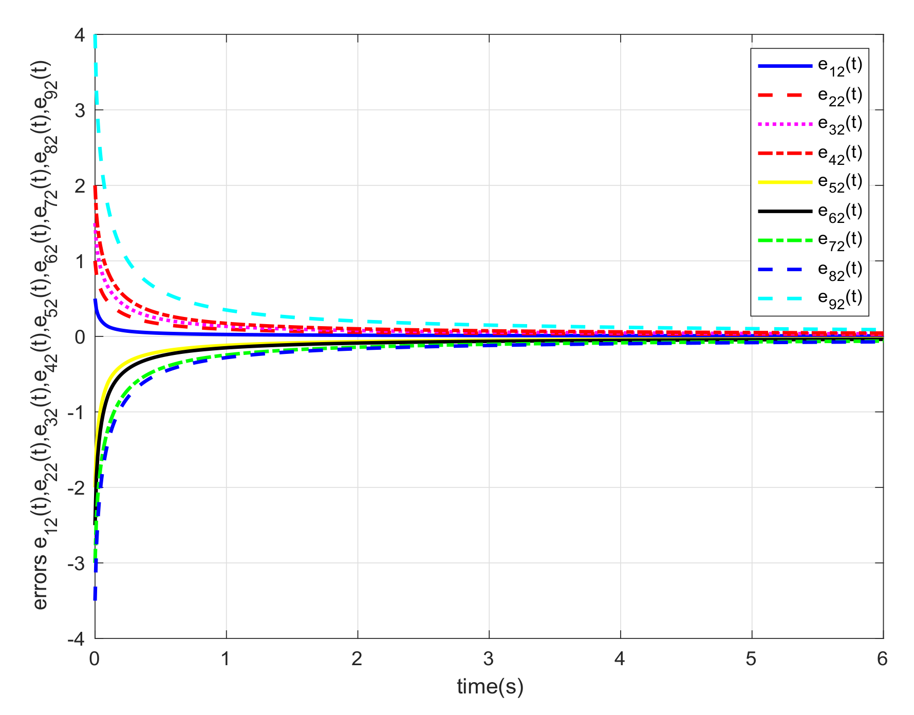
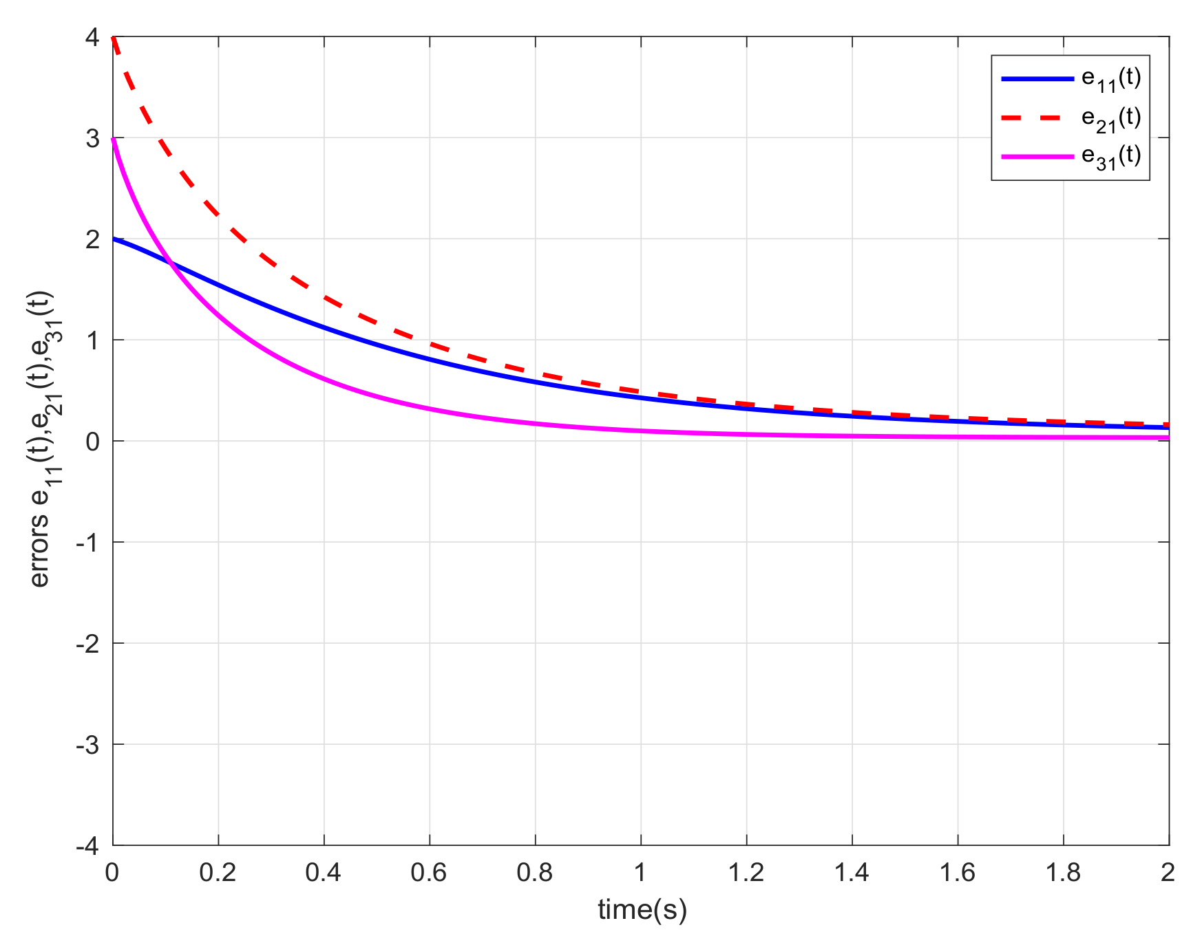
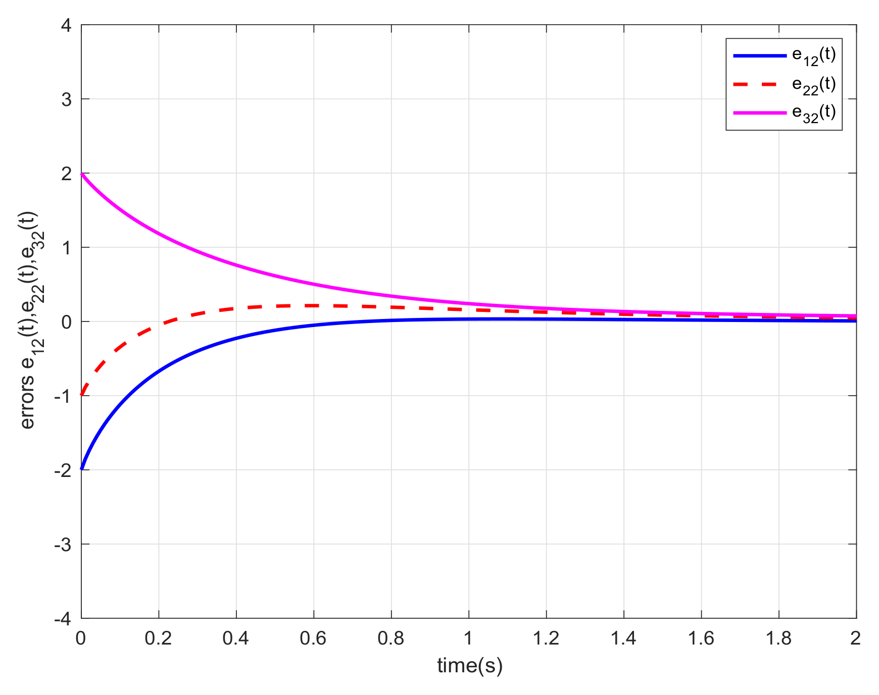
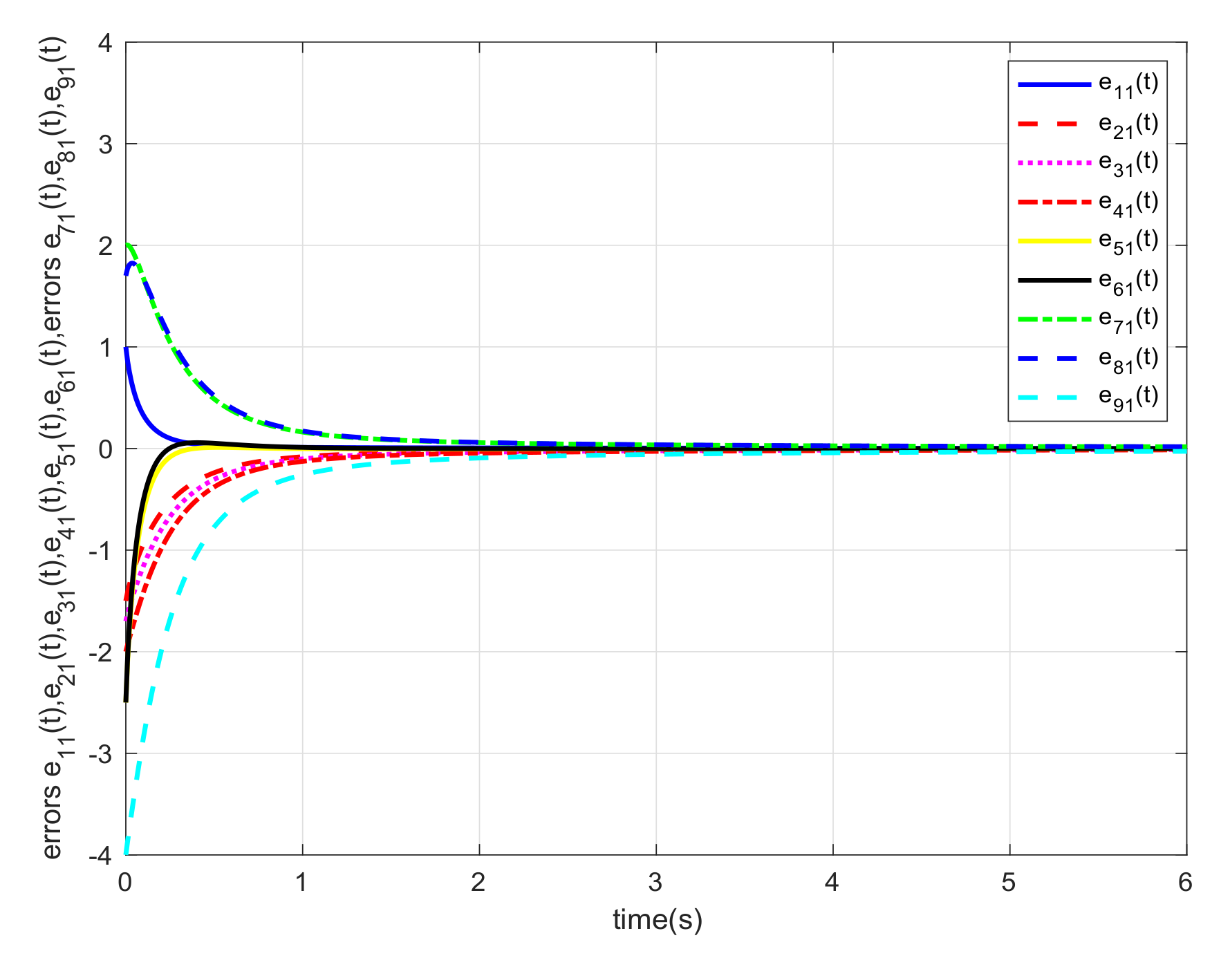
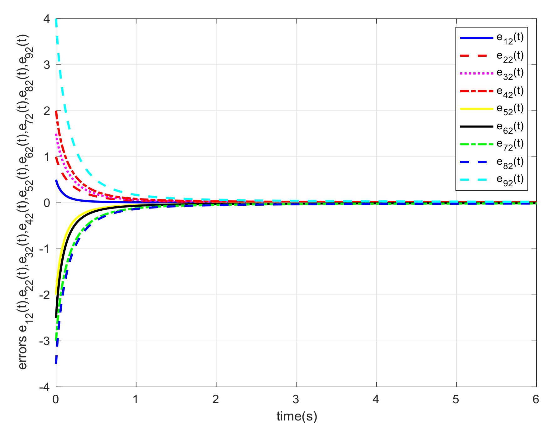
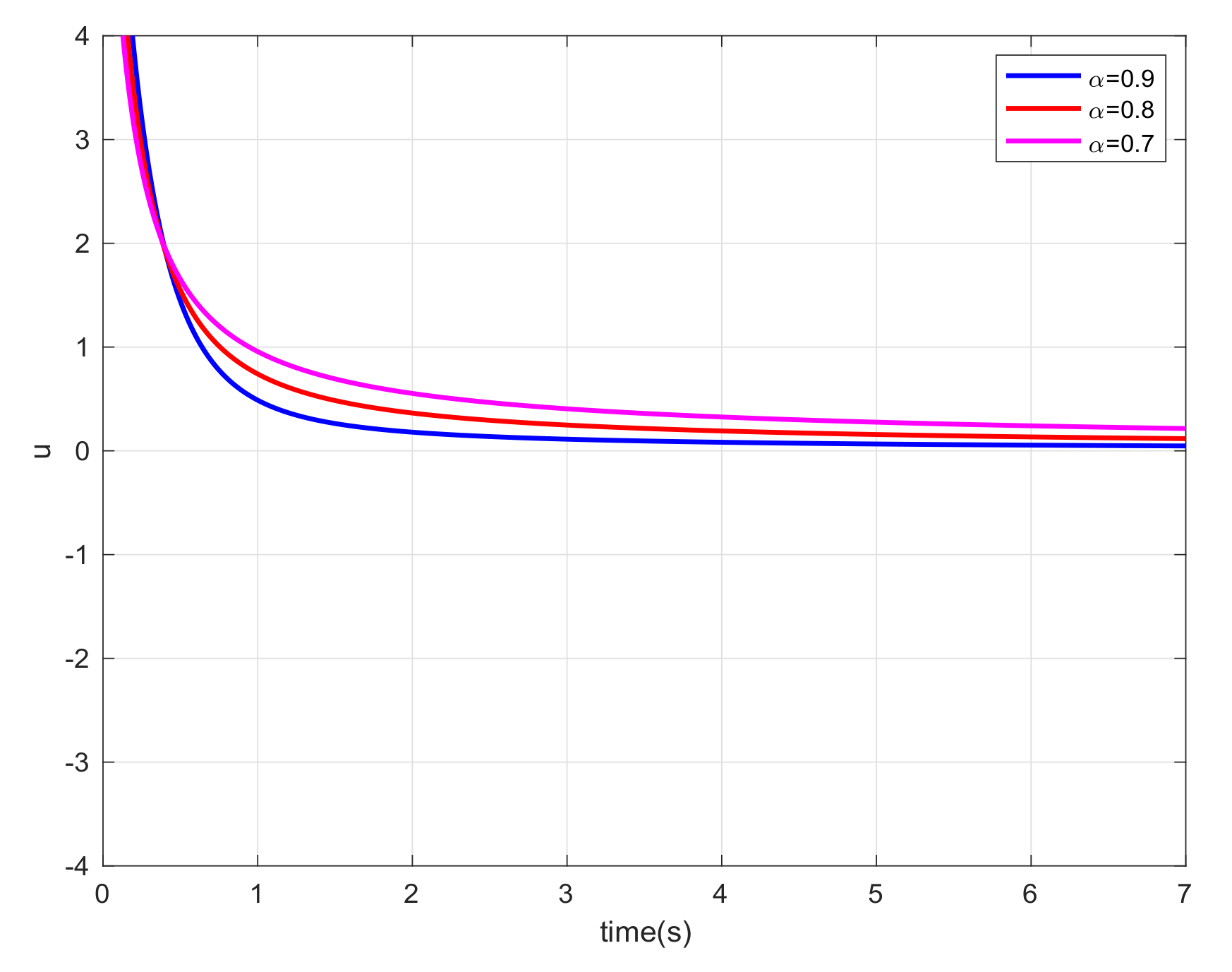
4. Numerical Simulations

In this section two examples are presented to verify the applicability and effectiveness of the scheme proposed.

Example 1.

Consider the undirected graph topology depicted in Figure 1. The matrices L and $\tilde{L}$ are given by the following:

$$L=\left[\begin{array}{cccc}1& -1& 0& 0\\ -1& 3& -1& -1\\ 0& -1& 2& -1\\ 0& -1& -1& 2\end{array}\right],\tilde{L}=\left[\begin{array}{ccc}4& -1& -1\\ 0& 2& -1\\ 0& -1& 2\end{array}\right]$$

and the parameters of each multi-agent are stated as follows.

$$\begin{array}{c}A = \left[\begin{array}{cc}-3& -2\\ 1& -4\end{array}\right], A_{\tau } = \left[\begin{array}{cc}0.2& 0.1\\ -0.1& 0\end{array}\right], B = \left[\begin{array}{c}0.2\\ -0.2\end{array}\right],\hfill \\ E_1 = \left[\begin{array}{c}0.1\\ 0.1\end{array}\right], F_1 = \left[\begin{array}{cc}0.2& -0.3\end{array}\right], F_2 = \left[\begin{array}{cc}-0.1& 0.2\end{array}\right],\hfill \\ \alpha = 0.9,\tau =0.1, F_3=-0.1, f\left(x\left(t\right)\right)=sin\left(x\left(t\right)\right).\hfill \end{array}$$

Figure 1. Topology of the system in Example 1.

It follows from Theorem 1 that the matrix $\overline{P}$, constant λ and gain matrix K can be obtained as the following.

$$\begin{array}{ccc}\hfill \overline{P}& =& \left[\begin{array}{cc}0.4441& -0.0221\\ -0.0221& 0.3075\end{array}\right],\lambda =1.1251,\hfill \end{array}$$

$$\begin{array}{c}\hfill K=Y{\overline{P}}^{-1}=\left[\begin{array}{cc}0.0556& 0.0003\end{array}\right].\end{array}$$

Let us choose $h\left(t\right)=cos\left(t\right)$ and the initial states $x_1\left(0\right)={[1,2]}^T$, $x_2\left(0\right)={[3,0]}^T$, $x_3\left(0\right)={[5,1]}^T$ and $x_4\left(0\right)={[4,4]}^T$. For different orders α, we also carried out the simulations and gave the corresponding error trajectories of this system. When order $\alpha =0.9,0.8,0.7$, we show the consensus errors versus time of the agents in Figure 2, Figure 3, Figure 4, Figure 5, Figure 6 and Figure 7, respectively. From the numerical results, we verify that $e_{1i}\left(t\right)$ and $e_{2i}\left(t\right)$ tend fast to 0, which means that the guaranteed cost consensus of the system $\left(\right)$ can be achieved. The upper bound of the guaranteed cost function $J^{*}=17.0088(\alpha =0.9)$ can be obtained. Moreover, by denoting $\parallel e\left(t\right)\parallel =\sqrt{{\sum }_i^n{e}_{ij}^2\left(t\right)}(j=1,2,\cdots ,n)$, we also carried out the curve of $\parallel e\left(t\right)\parallel$. From Figure 8, we could note that the order influence on consensus property with varying orders. With the higher orders, the system consensus’s error will be achieved more rapidly.

Figure 2. Error response $e_{i1}\left(t\right)$ of the system in Example 1 with $\alpha =0.9$.

Figure 3. Error response $e_{i2}\left(t\right)$ of the system in Example 1 with $\alpha =0.9$.

Figure 4. Error response $e_{i1}\left(t\right)$ of the system in Example 1 with $\alpha =0.8$.

Figure 5. Error response $e_{i2}\left(t\right)$ of the system in Example 1 with $\alpha =0.8$.

Figure 6. Error response $e_{i1}\left(t\right)$ of the system in Example 1 with $\alpha =0.7$.

Figure 7. Error response $e_{i2}\left(t\right)$ of the system in Example 1 with $\alpha =0.7$.

Figure 8. Error response $\parallel e\left(t\right)\parallel$ of the system in Example 1.

Example 2.

Consider the undirected graph represented in Figure 9. The matrices L and $\tilde{L}$ are the following:

$$\begin{array}{ccc}\hfill L& =& \left[\begin{array}{cccccccccc}3& -1& -1& -1& 0& 0& 0& 0& 0& 0\\ -1& 3& -1& 0& 0& 0& -1& 0& 0& 0\\ -1& -1& 5& -1& 0& -1& 0& -1& 0& 0\\ -1& 0& -1& 3& -1& 0& 0& 0& 0& 0\\ 0& 0& 0& -1& 3& -1& 0& 0& 0& -1\\ 0& 0& -1& 0& -1& 4& 0& 0& -1& -1\\ 0& -1& 0& 0& 0& 0& 2& -1& 0& 0\\ 0& 0& -1& 0& 0& 0& -1& 3& -1& 0\\ 0& 0& 0& 0& 0& -1& 0& -1& 3& -1\\ 0& 0& 0& 0& -1& -1& 0& 0& -1& 3\end{array}\right],\hfill \end{array}$$

$$\begin{array}{ccc}\hfill \tilde{L}& =& \left[\begin{array}{ccccccccc}2& -1& 0& 0& 0& 1& 0& 0& 0\\ 0& 4& 1& 0& 1& 0& 1& 0& 0\\ 0& 0& 2& 1& 0& 0& 0& 0& 0\\ -1& -1& 0& 3& 1& 0& 0& 0& 1\\ -1& 0& -1& 1& 4& 0& 0& 1& 1\\ 0& -1& -1& 0& 0& 2& 1& 0& 0\\ -1& 0& -1& 0& 0& 1& 3& 1& 0\\ -1& -1& -1& 0& 1& 0& 1& 3& 1\\ -1& -1& -1& 1& 1& 0& 0& 1& 3\end{array}\right]\hfill \end{array}$$

and the parameters of every agent are given by the following.

$$\begin{array}{ccc}\hfill A& =& \left[\begin{array}{cc}-7& -5\\ -1& -6\end{array}\right],A_{\tau }=\left[\begin{array}{cc}0.1& 0.3\\ -0.2& 0.1\end{array}\right],B=\left[\begin{array}{c}0.1\\ -0.4\end{array}\right],\hfill \\ \hfill E_1& =& \left[\begin{array}{c}0.4\\ 0.1\end{array}\right],F_1=\left[\begin{array}{cc}0.1& -0.2\end{array}\right],F_2=\left[\begin{array}{cc}0.3& -0.1\end{array}\right],\hfill \\ \hfill \alpha & =& 0.8,\tau =0.1,F_3=-0.4.\hfill \end{array}$$

Figure 9. Topology of the system in Example 2.

From Corollary 1, the matrix $\overline{P}$, constant λ and gain matrix K can be obtained as follows.

$$\begin{array}{ccc}\hfill \overline{P}& =& \left[\begin{array}{cc}0.1318& 0.0187\\ 0.0187& 0.0284\end{array}\right],\lambda =0.8642\hfill \end{array}$$

$$\begin{array}{c}\hfill K=Y{\overline{P}}^{-1}=\left[\begin{array}{cc}0.0918& 0.0062\end{array}\right].\end{array}$$

Let us select $h\left(t\right)=sin\left(t\right)$ and the initial states $x_1\left(0\right)={[1,0]}^T$, $x_2\left(0\right)={[2,2]}^T$, $x_3\left(0\right)={[5,-1]}^T$ and $x_4\left(0\right)={[-3,-2]}^T$. Similar with Example 1, we also carried out consensus error curve of system with different order. The simulation results are shown in the Figure 10, Figure 11, Figure 12, Figure 13, Figure 14 and Figure 15, respectively. From these numerical results, we verify that $e_{1i}\left(t\right)$ and $e_{2i}\left(t\right)$ approach 0 very fast, meaning that the guaranteed cost consensus of the system $\left(\right)$ is obtained. Additionally, the upper bound of the guaranteed cost function is $J^{*}=0.5502(\alpha =0.8)$. By plotting the curve of $\parallel e\left(t\right)\parallel$ shown in Figure 16, one can note that the system will achieve consensus more rapidly when the order increases.

Figure 10. Error response $e_{i1}\left(t\right)$ of the system in Example 2 with $\alpha =0.8$.

Figure 11. Error response $e_{i2}\left(t\right)$ of the system in Example 2 with $\alpha =0.8$.

Figure 12. Error response $e_{i1}\left(t\right)$ of the system in Example 2 with $\alpha =0.9$.

Figure 13. Error response $e_{i2}\left(t\right)$ of the system in Example 2 with $\alpha =0.9$.

Figure 14. Error response $e_{i1}\left(t\right)$ of the system in Example 2 with $\alpha =0.7$.

Figure 15. Error response $e_{i2}\left(t\right)$ of the system in Example 2 with $\alpha =0.7$.

Figure 16. Error response $\parallel e\left(t\right)\parallel$ of the system in Example 2.

5. Conclusions

The guaranteed cost consensus of uncertain delayed FOMASs with input delay was addressed in this paper. A guaranteed cost function related to FOMASs was proposed in order to consider the consensus regulation performance and the energy consumption simultaneously. By employing the FO Razumikhin theorem and the LMI approach, sufficient conditions on guaranteed cost and upper bounds for the guaranteed cost function were obtained. The proposed approach is order-dependent and delay-dependent, which results in less conservative conditions than those presented in alternative methods. It should be mentioned that taking the state and input delay as identical is unreasonable in real-world applications. However, since stability results for fractional-order systems with multiple time delays are unavailable, we considered this simplified case. Therefore, further work is needed to solve this problem. In addition, we will consider the guaranteed cost consensus of uncertain delayed FOMASs with order lying in (1,2) in our next work.

References

1. Yu, W.; Chen, G.; Wang, Z.; Yang, W. Distributed consensus filtering in sensor networks. IEEE Trans. Syst. Man Cybern. Part B (Cybern.) 2009, 39, 1568–1577. [Google Scholar]
2. Carpenter, J.R. A preliminary investigation of decentralized control far satellite formations. In Proceedings of the 2000 IEEE Aerospace Conference. Proceedings (Cat. No. 00TH8484), Big Sky, MT, USA, 25 March 2000; IEEE: Piscataway, NJ, USA, 2000; Volume 7, pp. 63–74. [Google Scholar]
3. McLain, T.W.; Chandler, P.R.; Rasmussen, S.; Pachter, M. Cooperative control of UAV rendezvous. In Proceedings of the 2001 American Control Conference, (Cat. No. 01CH37148), Arlington, VA, USA, 25–27 June 2001; IEEE: Piscataway, NJ, USA, 2001; Volume 3, pp. 2309–2314. [Google Scholar]
4. Hong, Y.; Hu, J.; Gao, L. Tracking control for multi-agent consensus with an active leader and variable topology. Automatica 2006, 42, 1177–1182. [Google Scholar] [CrossRef] [Green Version]
5. Tang, Y.; Gao, H.; Zhang, W.; Kurths, J. Leader-following consensus of a class of stochastic delayed multi-agent systems with partial mixed impulses. Automatica 2015, 53, 346–354. [Google Scholar] [CrossRef]
6. Kim, H.; Shim, H.; Seo, J.H. Output consensus of heterogeneous uncertain linear multi-agent systems. IEEE Trans. Autom. Control 2010, 56, 200–206. [Google Scholar] [CrossRef]
7. Zhu, W.; Jiang, Z.P.; Feng, G. Event-based consensus of multi-agent systems with general linear models. Automatica 2014, 50, 552–558. [Google Scholar] [CrossRef]
8. Zheng, Y.; Ma, J.; Wang, L. Consensus of hybrid multi-agent systems. IEEE Trans. Neural Netw. Learn. Syst. 2017, 29, 1359–1365. [Google Scholar] [CrossRef] [Green Version]
9. Yang, H.y.; Zhu, X.l.; Cao, K.c. Distributed coordination of fractional order multi-agent systems with communication delays. Fract. Calc. Appl. Anal. 2014, 17, 23–37. [Google Scholar] [CrossRef]
10. Peng, Z.; Wang, D.; Wang, H.; Wang, W. Distributed coordinated tracking of multiple autonomous underwater vehicles. Nonlinear Dyn. 2014, 78, 1261–1276. [Google Scholar] [CrossRef]
11. Chen, L.; Yin, H.; Huang, T.; Yuan, L.; Zheng, S.; Yin, L. Chaos in fractional-order discrete neural networks with application to image encryption. Neural Netw. 2020, 125, 174–184. [Google Scholar] [CrossRef]
12. Yang, R.; Liu, S.; Tan, Y.Y.; Zhang, Y.J.; Jiang, W. Consensus analysis of fractional-order nonlinear multi-agent systems with distributed and input delays. Neurocomputing 2019, 329, 46–52. [Google Scholar] [CrossRef]
13. Shi, M.; Yu, Y.; Xu, Q. Delay-dependent consensus condition for a class of fractional-order linear multi-agent systems with input time-delay. Int. J. Syst. Sci. 2019, 50, 669–678. [Google Scholar] [CrossRef]
14. Ren, G.; Yu, Y.; Xu, C.; Hai, X. Consensus of fractional multi-agent systems by distributed event-triggered strategy. Nonlinear Dyn. 2019, 95, 541–555. [Google Scholar] [CrossRef]
15. Hu, T.; He, Z.; Zhang, X.; Zhong, S. Leader-following consensus of fractional-order multi-agent systems based on event-triggered control. Nonlinear Dyn. 2020, 99, 2219–2232. [Google Scholar] [CrossRef]
16. Gong, P.; Wang, K. Output feedback consensus control for fractional-order nonlinear multi-agent systems with directed topologies. J. Frankl. Inst. 2020, 357, 1473–1493. [Google Scholar] [CrossRef]
17. Gong, P.; Wang, K.; Lan, W. Fully distributed robust consensus control of multi-agent systems with heterogeneous unknown fractional-order dynamics. Int. J. Syst. Sci. 2019, 50, 1902–1919. [Google Scholar] [CrossRef]
18. Hu, W.; Wen, G.; Rahmani, A.; Bai, J.; Yu, Y. Leader-following consensus of heterogenous fractional-order multi-agent systems under input delays. Asian J. Control 2020, 22, 2217–2228. [Google Scholar] [CrossRef]
19. Ren, G.; Yu, Y. Consensus of fractional multi-agent systems using distributed adaptive protocols. Asian J. Control 2017, 19, 2076–2084. [Google Scholar] [CrossRef]
20. Wyrwas, M.; Mozyrska, D.; Girejko, E. Fractional discrete-time consensus models for single-and double-summator dynamics. Int. J. Syst. Sci. 2018, 49, 1212–1225. [Google Scholar] [CrossRef]
21. Yaghoubi, Z.; Talebi, H.A. Consensus tracking for nonlinear fractional-order multi-agent systems using adaptive sliding mode controller. Mechatron. Syst. Control (Former Control Intell. Syst.) 2019, 47, 194–200. [Google Scholar] [CrossRef]
22. Wei, Z.; Bo, C. Leader-following consensus of fractional-order multi-agent systems with nonlinear models. Appl. Math. Mech. 2015, 36, 555–562. [Google Scholar]
23. Luo, Y.; Xiao, X.; Cao, J.; Li, A. Event-triggered guaranteed cost consensus for uncertain nonlinear multi-agent systems with time delay. Neurocomputing 2020, 394, 13–26. [Google Scholar] [CrossRef]
24. Wang, Z.; Fan, Z.; Liu, G. Guaranteed performance consensus problems for nonlinear multi-agent systems with directed topologies. Int. J. Control 2019, 92, 2952–2962. [Google Scholar] [CrossRef]
25. Wang, Z.; Xi, J.; Yao, Z.; Liu, G. Guaranteed cost consensus for multi-agent systems with fixed topologies. Asian J. Control 2015, 17, 729–735. [Google Scholar] [CrossRef]
26. Wang, Z.; Xi, J.; Yu, Z.; Liu, G. Guaranteed cost consensus for multi-agent systems with time delays. J. Frankl. Inst. 2015, 352, 3612–3627. [Google Scholar] [CrossRef]
27. Liu, J.; Zhang, Y.; Sun, C.; Yu, Y. Fixed-time consensus of multi-agent systems with input delay and uncertain disturbances via event-triggered control. Inf. Sci. 2019, 480, 261–272. [Google Scholar] [CrossRef]
28. Xie, L. Output feedback H control of systems with parameter uncertainty. Int. J. Control 1996, 63, 741–750. [Google Scholar] [CrossRef]
29. Liang, S.; Wu, R.; Chen, L. Comparison principles and stability of nonlinear fractional-order cellular neural networks with multiple time delays. Neurocomputing 2015, 168, 618–625. [Google Scholar] [CrossRef]
30. Ni, W.; Cheng, D. Leader-following consensus of multi-agent systems under fixed and switching topologies. Syst. Control Lett. 2010, 59, 209–217. [Google Scholar] [CrossRef]
31. Chen, L.; Li, T.; Wu, R.; Lopes, A.M.; Machado, J.T.; Wu, K. Output-feedback guaranteed-cost control of fractional-order uncertain linear delayed systems. Comput. Appl. Math. 2020, 39, 210. [Google Scholar] [CrossRef]
32. Shen, B.; Wang, Z.; Tan, H. Guaranteed cost control for uncertain nonlinear systems with mixed time-delays: The discrete-time case. Eur. J. Control 2018, 40, 62–67. [Google Scholar] [CrossRef]
33. Xi, J.; Fan, Z.; Liu, H.; Zheng, T. Guaranteed-cost consensus for multiagent networks with Lipschitz nonlinear dynamics and switching topologies. Int. J. Robust Nonlinear Control 2018, 28, 2841–2852. [Google Scholar] [CrossRef] [Green Version]
34. Chen, B.; Chen, J. Razumikhin-type stability theorems for functional fractional-order differential systems and applications. Appl. Math. Comput. 2015, 254, 63–69. [Google Scholar] [CrossRef]
35. Chen, Y.; Wen, G.; Peng, Z.; Huang, T.; Yu, Y. Necessary and sufficient conditions for group consensus of fractional multiagent systems under fixed and switching topologies via pinning control. IEEE Trans. Cybern. 2019, 51, 28–39. [Google Scholar] [CrossRef] [PubMed]
36. Zhu, W.; Chen, B.; Yang, J. Consensus of fractional-order multi-agent systems with input time delay. Fract. Calc. Appl. Anal. 2017, 20, 52. [Google Scholar] [CrossRef]
37. Wang, X.; Li, X.; Huang, N.; O’Regan, D. Asymptotical consensus of fractional-order multi-agent systems with current and delay states. Appl. Math. Mech. 2019, 40, 1677–1694. [Google Scholar] [CrossRef]