Dynamics of Fractional-Order Digital Manufacturing Supply Chain System and Its Control and Synchronization

Abstract

Digital manufacturing is widely used in the production of automobiles and aircrafts, and plays a profound role in the whole supply chain. Due to the long memory property of demand, production, and stocks, a fractional-order digital manufacturing supply chain system can describe their dynamics more precisely. In addition, their control and synchronization may have potential applications in the management of real-word supply chain systems to control uncertainties that occur within it. In this paper, a fractional-order digital manufacturing supply chain system is proposed and solved by the Adomian decomposition method (ADM). Dynamical characteristics of this system are studied by using a phase portrait, bifurcation diagram, and a maximum Lyapunov exponent diagram. The complexity of the system is also investigated by means of SE complexity and $C_0$ complexity. It is shown that the complexity results are consistent with the bifurcation diagrams, indicating that the complexity can reflect the dynamical properties of the system. Meanwhile, the importance of the fractional-order derivative in the modeling of the system is shown. Moreover, to further investigate the dynamics of the fractional-order supply chain system, we design the feedback controllers to control the chaotic supply chain system and synchronize two supply chain systems, respectively. Numerical simulations illustrate the effectiveness and applicability of the proposed methods.

1. Introduction

Fractional-order calculus is an extension and generalization of integer-order calculus, and fractional-order differential equations are obtained by acting the fractional-order differential operators on integer-order ones. Although the theory of fractional-order calculus had been proposed 300 years ago, and it developed slowly for a long time due to its lack of practical engineering application background and its large computational size, it now attracts extensive attention due to increases in computational power. It was not until Mandelbrot [1] first pointed out the fact that fractional dimension exists in nature and in many fields of science and technology in 1983 that the application of fractional-order calculus attracted wide attention and developed rapidly. Fractional order systems have long memory of history data [2,3]. The classical derivative in one point is only affected by the information in the local neighborhood of that point, while the fractional derivative in one point is affected by the combination of all of the information of the model in historical moments. Therefore, compared with integer-order calculus, fractional-order calculus produces more accurate and reliable results for modelling of real-world systems due to the memory effect. Recently, fractional-order systems have received special attention from researchers in various fields such as physics [4], biology [5], neural network [6], management, and economics [7,8,9,10,11], etc. On the other hand, chaos theory and applied research have developed rapidly and promoted its significant contribution in various scientific fields [12]. Nowadays, the control and synchronization of nonlinear systems are the focus of many research studies in a variety of fields [13,14,15]. Some effective controllers have been designed to control and synchronize the fractional-order chaotic systems such as the coupling controller [16], adaptive controllers [17], linear feedback controllers [18], sliding mode controllers [19], fractional order PID controllers [20,21], and so on.

Supply chain systems are complex dynamic systems with various uncertainties [22,23]. In recent years, some researchers [24,25,26,27,28] are studying nonlinear chaotic dynamics of supply chain systems and have obtained many investigations. Forrester [29] was the first to investigate the dynamics of supply chain systems and introduced the ‘bullwhip effect’. The ‘bullwhip effect’ refers to the distortion of information in the process of transmitting information from downstream to upstream enterprises, and the distortion and gradual amplification of information in the process of transmitting information from the final customer to the original supplier in the supply chain, resulting in the phenomenon of cascading demand information. The ‘bullwhip effect’ can be explained by the chaos theory of dynamical systems. One of the most fundamental characteristics of chaos is that the trajectory of the system is very sensitive to the initial condition, i.e., even if the original state changes slightly, the final state of the system can be very different. Goksu et al. [30] constructed a supply chain model composed of manufacturers, distributors, and customers to achieve the synchronization and control of this chaotic supply chain management system. Gao et al. [31] proposed a new three-dimensional supply chain fractional-order difference game model composed of manufacturers, distributors, and retailers, and used the correlation theory of fractional-order difference to numerically analyze the complex dynamic behavior of this model, and discuss the effect of the output adjustment speed parameter on the dynamic behavior of the system. Recently, Yan et al. [32] integrated the computer-aided digital manufacturing process into the three-level supply chain which is composed of manufacturers, distributors, and retailers, and considered computer-aided digital design prior to the production by manufacturers, ultimately achieving synchronization and control of the system.

There are numerous attribute properties that cannot be described by the theory of integer-order calculus, so it is necessary to theoretically study the complexity of the supply chain system using the method of bifurcation and chaos of fractional nonlinear dynamics. In a supply chain system, the variables including demand, supply, and production have long memory properties, the fluctuation of which can lead to significant instability in the operation and delivery of the system. Thus, the traditional integer-order supply chain model has limitations to accurately show the operation of the system. Moreover, the prevalence of the bullwhip effect in the supply chain management increases the risks of production, supply, inventory management and marketing of suppliers, and even leads to chaos in them. However, there are few results on fractional-order supply chain systems.

Motivated by the above discussions, to be more realistic, in this study, a fractional-order digital manufacturing supply chain system is investigated. Dynamics and complexity of this system with the variation of derivative orders and system parameter have been studied by means of bifurcation diagram and complexity measure algorithms. Furthermore, the nonlinear feedback controllers are designed to control and synchronize the chaos in this fractional order supply chain system, respectively. That is, the fractional order supply chain system has rich dynamic behaviors, and the evolution simulation is conducted for the influence of the change of fractional order and parameters on the demand order quantity, supply quantity, and digital manufacturing quantity of the supply chain enterprises. At the same time, the chaotic states appearing in the evolution process are synchronized and controlled to achieve the stability of the supply chain system. Therefore, this study contains both theoretical and practical guidance to eliminate chaotic dynamics that are unfavorable to the supply chain model.

The rest of this paper is organized as follows. In Section 2, preliminaries and modeling are investigated. In Section 3, the dynamical behaviors of fractional-order digital manufacturing supply chain system are studied. In Section 4, controllers are designed to synchronize two identical systems. In Section 5, we consider the stabilization of the system. This paper ends with a conclusion in Section 6.

2. Preliminaries and Modeling

2.1. Preliminaries

In order to solve fractional-order calculus equations, various definitions of fractional-order calculus have been proposed, among which the most common ones are the Grunwald-Letnikov (G-L) fractional-order calculus definition, the Riemann-Liouville (R-L) fractional-order calculus definition, and the Caputo fractional-order calculus definition [33]. The algorithm based on the Caputo definition has clear physical meaning and is beneficial to solve the actual physical system, having more practical engineering applications. In this paper, we will only use the Caputo fractional derivative.

Definition 1.

The Caputo fractional derivative of order$q$is given by

$${}_a{}^{C}D_t^{q}f(t)=\frac{1}{\Gamma (n-1)}{\int }_a^t{(t-\tau )}^{n-q-1}{f}^{\left(n\right)}(\tau )\mathrm{d}\tau ,$$

(1)

where $n-1<q<n$, $a$ and $t$ are numbers representing the limits of the operator ${}_a{}^{C}D_t^q$, and the symbol $\Gamma (\cdot )$ is the gamma function.

Lemma 1

([34]). Consider the following fractional-order system:

$$\frac{{\mathrm{d}}^{q}x(t)}{\mathrm{d}{t}^q}=f(x(t)),x(0)=x_0\in {ℝ}^N,q\in (0,1),$$

(2)

where $x(t)={\left(x_1(t),x_2(t),\dots ,x_N(t)\right)}^T\in {ℝ}^N$ and $f:{\left[f_1,f_2,\dots ,f_N\right]}^T:{ℝ}^N\to {ℝ}^N$. The equilibrium points of the above system are solutions to the equation $f(x(t))=0$. An equilibrium is asymptotically stable if all eigenvalues ${\lambda }_i$ of the Jacobian matrix $J=\frac{\partial f}{\partial x}=\frac{\partial \left(f_1,f_2,\dots ,f_N\right)}{\partial \left(x_1,x_2,\dots ,x_N\right)}$ evaluated at the equilibrium satisfy $\left|\arg ({\lambda }_i)\right|>\frac{\pi q}{2}$.

As for the fractional-order continuous systems, there are several different solution algorithms such as the frequency domain method (FDM) [35], the Adams-Bashforth-Moulton algorithm (ABM) [36], and the Adomian decomposition method (ADM) [37]. The ADM has higher accuracy and smaller computational error compared to the prediction-correction algorithm and the Runge-Kutta algorithm [38], and it is used in this paper.

For a given fractional-order chaotic system with form of $D_{t_0}^{q}x(t)=f(x(t))+g(t)$, where $x(t)={\left[x_1(t),x_2(t),\dots ,x_n(t)\right]}^{{\rm T}}$ is the state variable, $g(t)=[g_1(t),g_2(t),\dots ,$ $g_n(t)]$ is the constant in the system, and $D_{t_0}^q$ is the Caputo fractional derivative operator. Then it can be divided into three parts as the form

$$D_{t_0}^{q}x(t)=Lx(t)+Nx(t)+g(t),$$

(3)

where $m\in N$, $m-1<q\le m$. $Lx(t)$ and $Nx(t)$ are the linear and nonlinear terms of the fractional differential equations respectively. Then, let $J_{t_0}^q$ is the inverse operator of $D_{t_0}^q$, thus we have

$$x=J_{t_0}^{q}Lx+J_{t_0}^{q}Nx+J_{t_0}^{q}g+\mathsf{\Phi }$$

(4)

where $\mathsf{\Phi }={\displaystyle \sum _{k=0}^{m-1}}{\mathbf{b}}_k\frac{{(t-t_0)}^k}{k!}$, ${\mathbf{x}}^{\left(k\right)}\left(t_0^{+}\right)={\mathbf{b}}_k$, $k=0,\cdots ,m-1$, and it involves the initial condition. By applying the recursive relation

$$\{\begin{array}{l}{x}^0=J_{t_0}^{q}g+\mathsf{\Phi }\hfill \\ x^1=J_{t_0}^{q}L{x}^0+J_{t_0}^q{A}^0\left(x^0\right)\hfill \\ x^2=J_{t_0}^{q}L{x}^1+J_{t_0}^q{A}^1\left(x^0,x^1\right)\hfill \\ \cdots \hfill \\ x^i=J_{t_0}^{q}L{x}^{i-1}+J_{t_0}^q{A}^{i-1}\left(x^0,x^1,\cdots ,x^{i-1}\right)\hfill \\ \cdots \hfill \end{array},$$

(5)

The analytical solution of the fractional-order system is given by

$$\mathbf{x}(t)=\sum _{i=1}^{\infty }{\mathbf{x}}^i,$$

(6)

where $i=1,2,\dots ,\infty$, and the nonlinear terms of the fractional differential equations $Nx(t)$ are evaluated by

$$N\mathbf{x}=\underset{i=0}{{\sum }^{}^{\infty }}{\mathbf{A}}^i\left({\mathbf{x}}^0,{\mathbf{x}}^1,\cdots ,{\mathbf{x}}^i\right),$$

(7)

$$\left\{\begin{array}{c}{A}_j^i=\frac{1}{i!}{\left[\frac{d^i}{d{\lambda }^i}N\left(v_j^i\left(\lambda \right)\right)\right]}_{\lambda =0}\hfill \\ v_j^i\left(\lambda \right)={\displaystyle \sum _{k=0}^i}{\left(\lambda \right)}^k{x}_j^k\hfill \end{array}\right..$$

(8)

Nonlinear time series complexity measure is an important technique to analyze the dynamics of a chaotic system, and is currently a hot topic in the field of nonlinear research. Complexity measure of chaotic systems is to use some algorithms to measure how close the chaotic sequence is to the random sequence, and the complexity value is larger when the sequence is closer to the random sequence. There are several methods to measure the complexity of chaotic systems including statistical complexity measure (SCM), fuzzy entropy, sample entropy, spectral entropy (SE) [39], and $C_0$ algorithm [40]. Among these methods, SE and $C_0$ algorithms are proper methods to estimate the complexity of a time series accurately. So, SE and $C_0$ algorithms are used in this paper.

2.2. Modeling

In Ref. [32], Yan et al. designed a four-dimensional supply chain model, a demand-driven supply chain model based on digital manufacturing, focusing on the impact of digital manufacturing on manufacturers and then on the whole supply chain. The model is given by

$$\{\begin{array}{l}{x}^{\prime }=(m+{\theta }_m)y-(n+1+{\theta }_n)x,\\ y^{\prime }=(r+{\theta }_r)x-xw-y,\\ z^{\prime }=-(d+{\theta }_d)z+xy,\\ w^{\prime }=(c+{\theta }_c)(d+{\theta }_d)z-(k-1-{\theta }_k)w,\end{array}$$

(9)

where x is the demand order quantity by retailers for the products, $y$ is the supply quantity by distributors, $z$ is the quantity of finished computer aided digital design, $w$ is the quantity produced based on the digital design, $m$ is the delivery efficiency of distributors, $n$ is the rate of satisfying the retailer demand, $r$ is the rate of information distortion for the demand by retailers for the products, $d$ is the rate that the digital design is put into production, $c$ is the conversion rate from digital design to product, $k$ is the safety stock coefficient for manufacturers, and $({\theta }_m,{\theta }_n,{\theta }_r,{\theta }_d,{\theta }_c,{\theta }_k)$ denote the parameters of the perturbations on the system. In addition, $x<0$ indicates that the supply of distributors is less than retailer demand, and $w<0$ indicates that there is no new production due to backlogs or returns.

In a supply chain system, the variables including demand, supply, and production have a long memory property; since the integer-order difference calculus has no long-memory effect, its theory is not suitable for studying the supply chain system with long-memory effects. Thus, the traditional integer-order supply chain model has limitations to accurately show the operation of the system. In this paper, the Caputo fractional derivative operator is applied in system (9), then the supply chain system with computer aided digital manufacturing process in the form of fractional-order differential equations are obtained as

$$\{\begin{array}{l}{D}_t^{q}x=(m+{\theta }_m)y-(n+1+{\theta }_n)x\\ D_t^{q}y=(r+{\theta }_r)x-xw-y\\ D_t^{q}z=-(d+{\theta }_d)z+xy\\ D_t^{q}w=(c+{\theta }_c)(d+{\theta }_d)z-(k-1-{\theta }_k)w\end{array}$$

(10)

where $q\in \left(0,1\right)$ denotes the order of derivatives, in particular, model (10) degenerates to the integer-order supply chain differential equations when $q=1$. Here, we take the same order of the fractional derivative in all equations, and choose the parameters $m=0.9$, $n=0.8$, $r=64.7$, $c=1.4$, $k=4.8$, ${\theta }_m=0.1$, ${\theta }_n=0.2$, ${\theta }_r=0.3$, ${\theta }_d=0.1$, ${\theta }_c=0.2$, and ${\theta }_k=0.3$. Since this paper focuses on the impact of digital manufacturing process on the whole supply chain system, the parameter $d$ is taken as the control variable. Thus, the fractional-order supply chain system is proposed as follows

$$\{\begin{array}{l}{D}_t^{q}x=y-2x\\ D_t^{q}y=65x-xw-y\\ D_t^{q}z=-(d+0.1)z+xy\\ D_t^{q}w=(1.6d+0.16)z-3.5w\end{array}$$

(11)

Here, an approximate solution to the fractional-order value of the system (11) is ${\tilde{x}}_j=c_j^0+c_j^1\frac{{(t-t_0)}^q}{\Gamma (q+1)}+c_j^2\frac{{(t-t_0)}^{2q}}{\Gamma (2q+1)}+\dots +c_j^6\frac{{(t-t_0)}^{2q}}{\Gamma (6q+1)}$, $j=1,2,3,4$, and the detailed derivation of $c_j^1,,c,\cdots ,c_j^6$ is given in Appendix A.

3. Dynamics Analysis of the Fractional-Order Supply Chain System

With the variation of derivative orders and system parameters, system (11) has complex dynamic behaviors such as periodic motions, period-doubling motions, and chaotic motions. If the system behaves chaotically, the supply chain system will be in a state of loss of control, which will lead to inventory, ordering, and supply chaos, and affect the decision making of supply chain enterprises at all levels, thus causing greater damage to the operation of the whole supply chain system. If the system appears in a periodic state, the supply chain system will be stable and the supply chain enterprises can make decisions based on the inventory status better. Therefore, studying the chaotic dynamic behaviors of the supply chain system can be an effective means to maintain the stability of the supply chain system and guide the scientific decision making of the supply chain enterprises.

In this section, the numerical solution of system (11) is obtained by means of ADM, and the chaotic dynamic behaviors of the system with the variation of the fractional order q and the parameter $d$ are studied through bifurcation diagrams, maximum Lyapunov exponent diagrams, phase portraits, time series diagrams and complexity diagrams.

3.1. Dynamic Behaviors Analysis with Parameter $d$

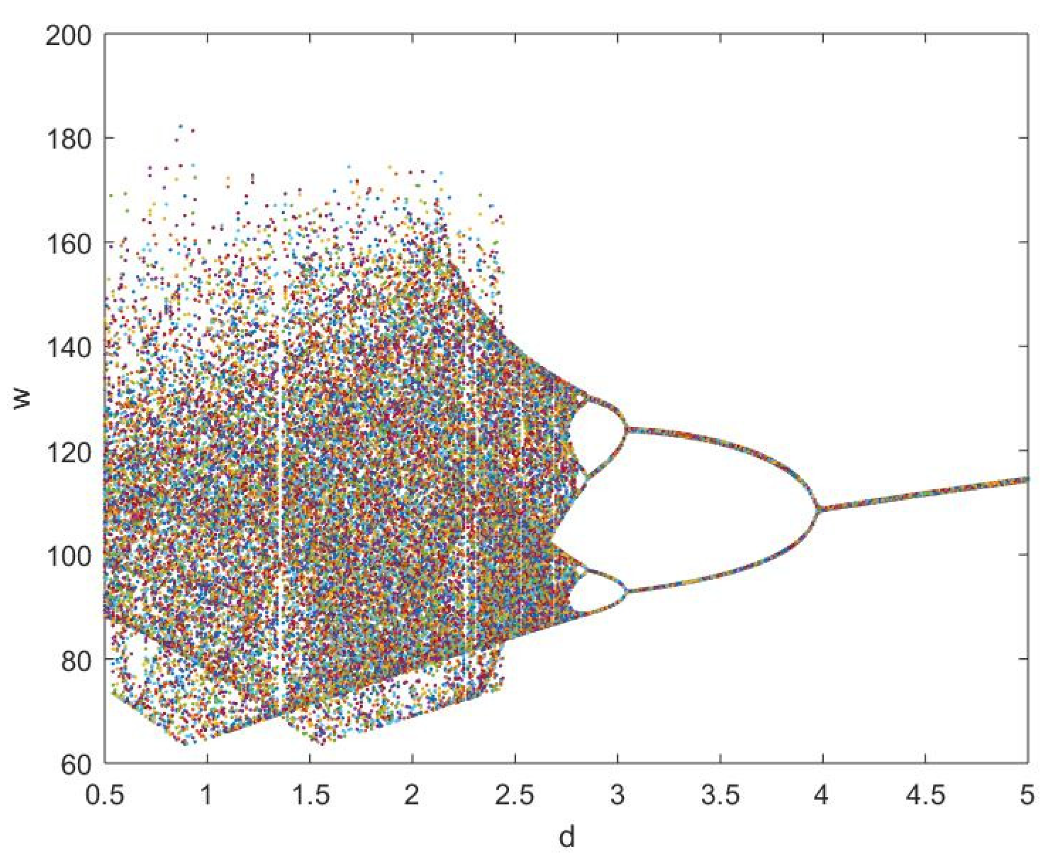
If a manufacturing company produces digitally, it will be followed by digital design into production. Moreover, the larger the parameter $d$, the higher the level of digital production. In this subsection, we study the impact of the rate of digital design into production on the manufacturer and the supply chain. 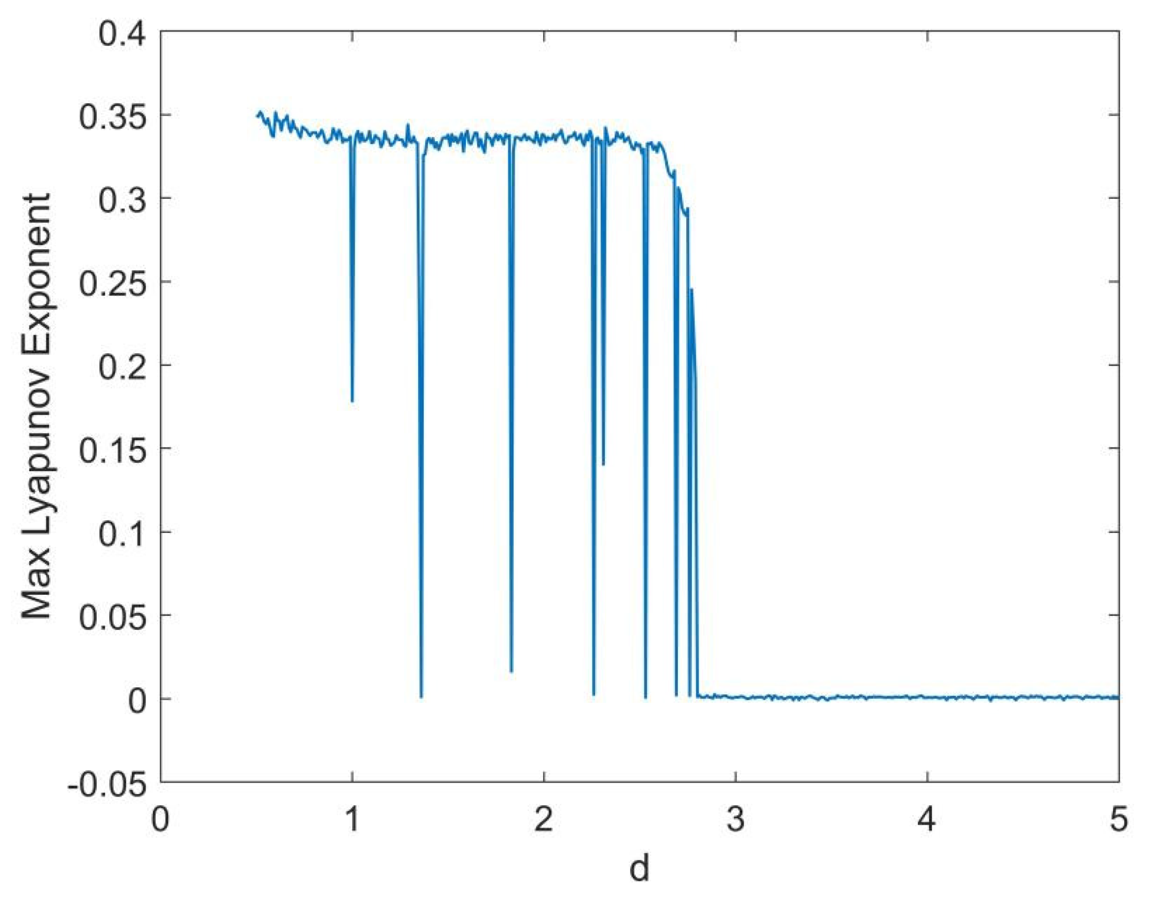In system (11), let the fractional order $q=0.75$, the initial conditions $(x_0,y_0,z_0,w_0)=(0.2,0.2,0.3,0.32)$, and the parameter $d$ is chosen as the critical variable. The bifurcation diagram and the maximum Lyapunov exponent diagram of system (11) with the parameter $d$ varying from 0.5 to 5 are shown in Figure 1 and Figure 2. The results indicate that the system shows the inverse period-doubling bifurcation, and as the parameter $d$ decreases, the system goes from periodic state, after the period-doubling bifurcation, to chaotic state. When $d\in \left[3.33,5\right]$, the period one is appeared, and the period-doubling bifurcation occurs for $d=3.33$. When $d\in \left[2.37,3.33\right)$, the period two is appeared, and the period-doubling bifurcation occurs for $d=2.37$. When $d\in \left[2.23,2.37\right)$, the period four is appeared, and the period-doubling bifurcation occurs for $d=2.23$. When $d<2.18$, the system enters to chaotic state, which can be illustrated from the maximum Lyapunov exponent.

The numerical simulation results can reflect the actual situation of the supply chain system. When the rate that the digital design is put into production is high, it means that the products are digitally produced quickly, hence the replenishment demand of retailers can be met immediately, and consequently the demand of consumers can be met quickly, making the inventory system and the production of manufacturers stable. On the contrary, when the rate is low, the order demand of retailers cannot be met in time, so consumers may seek other alternatives, which will lead to overstock and chaos in production. Therefore, the strategy to increase the rate of digital design into production is feasible and it can make the whole supply chain system stable.

In order to observe the dynamic behaviors of system (11) directly, the phase portraits of the system with several different values of the parameter d are shown in Figure 3. When $d=0.7$, the system is chaotic and the chaotic attractor is presented in Figure 3a. The numerical analysis shows that the interaction between the quantity of demand from retailers, the quantity of products available from distributors, the quantity of completed digital designs, and the quantity of production based on digital designs. When $d=2.9$, the system is in the periodic four that is shown in Figure 3b. When $d=3.5$, the period two is appeared, and it is shown in Figure 3c. When $d=4$, the periodic one of the system is presented in Figure 3d. The phase diagrams are consistent with the bifurcation diagram and the maximum Lyapunov exponent diagram. Thus, the fractional-order supply chain system has rich dynamical properties when the parameter $d$ of system (18) is varied.

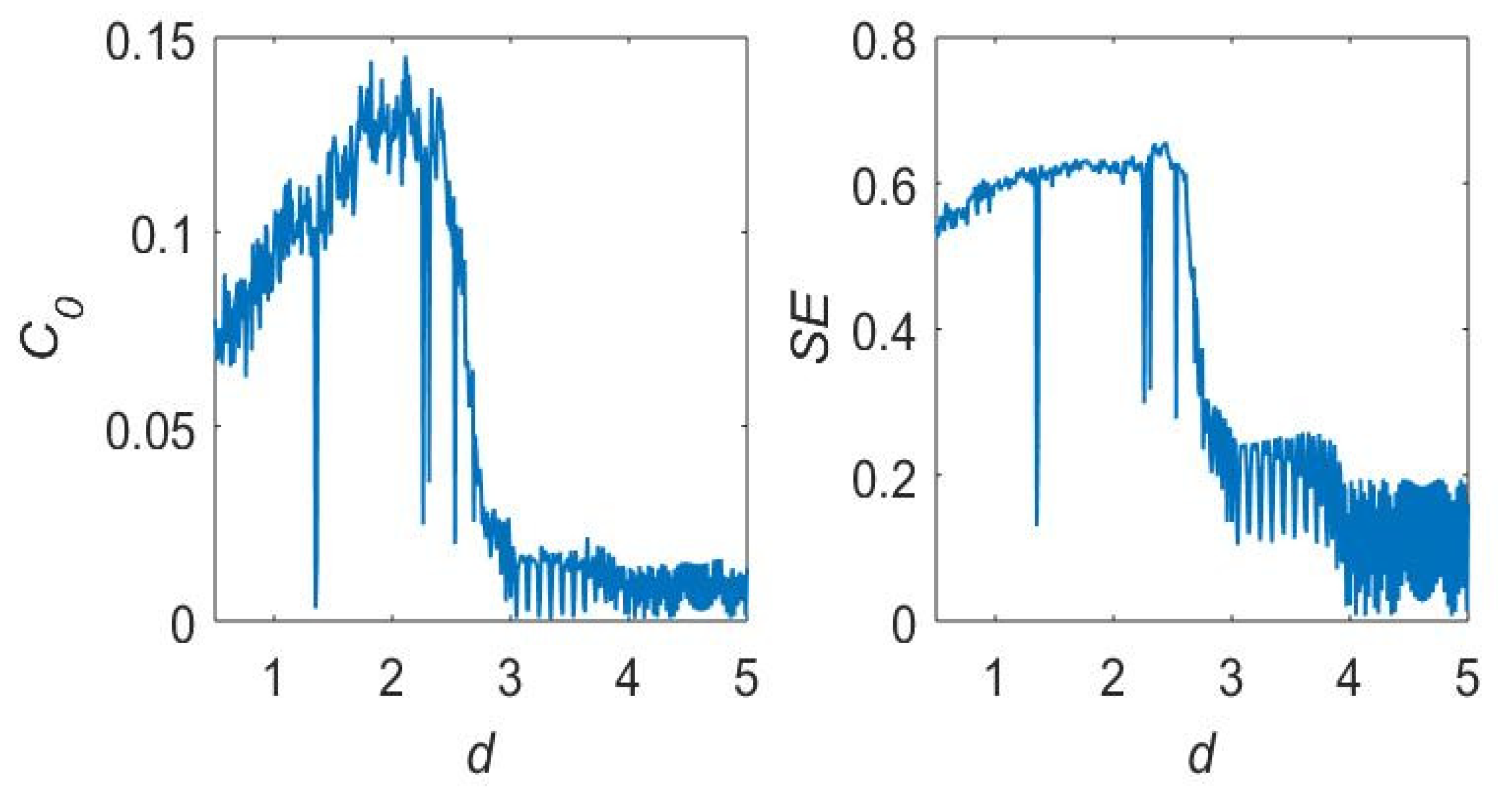
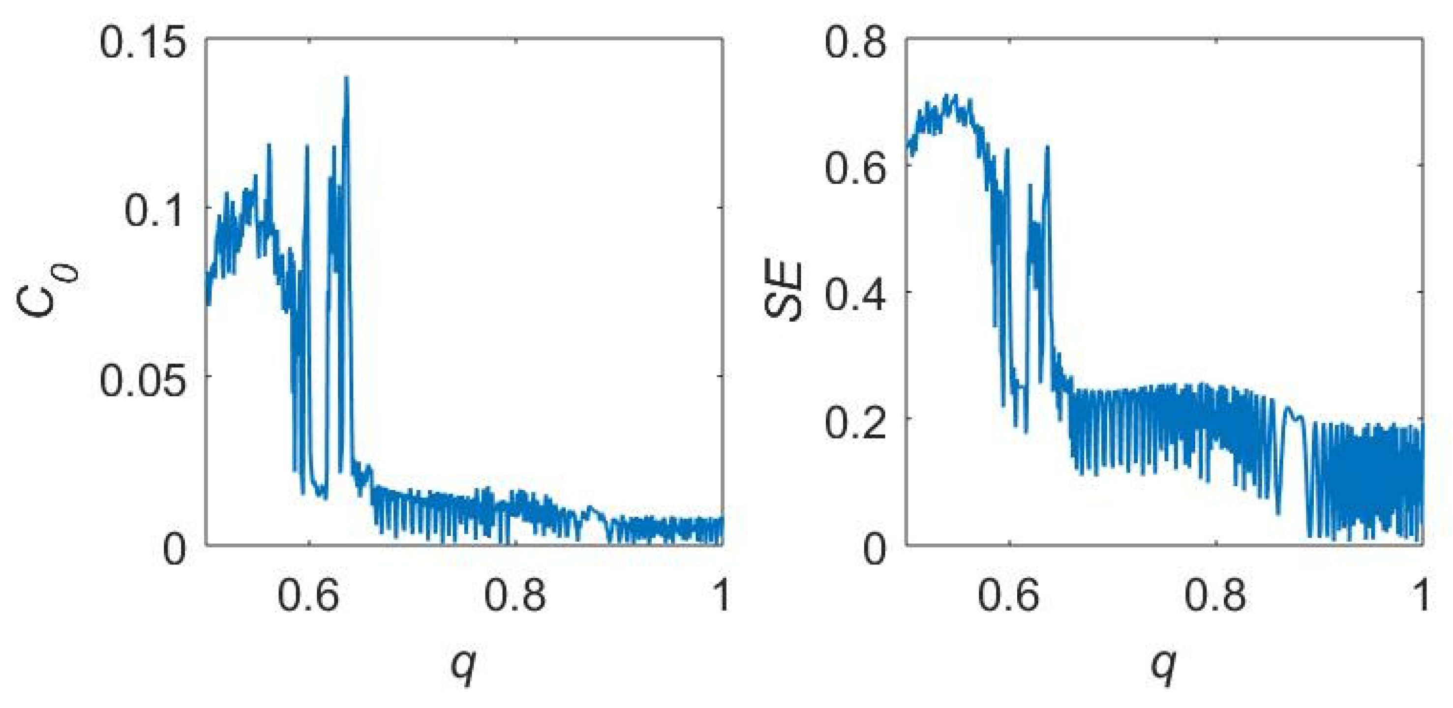
As shown in Figure 4, the $C_0$ complexity and SE complexity of system (18) have high values when $0.5<d<2.18$, indicating that production and inventory of manufacturers appear chaotic and difficult to predict; when $d\ge 2.18$, the value of the complexity is very small, indicating that it contributes to production planning of manufacturers and supply and inventory management of supply chain enterprises.

3.2. Dynamical Behaviors with $q$

In system (11), let the parameter $d=3.5$, the initial conditions $(x_0,y_0,z_0,w_0)=$ $\left(0.2,0.2,0.3,0.32\right)$ and the parameter $q$ is chosen as the critical variable to show the effect of fractional order to the behavior of chaotic system results. Figure 5 shows the bifurcation diagram with the order q as the bifurcation parameter. When $q\in \left[0.47,0.62\right]$, the system is mostly in a chaotic state. When $q>0.62$, the chaos disappears and the system appears in a periodic state. In order to study the effect of different fractional orders on the supply chain system when manufacturers have a high rate of digital design into production, we consider choosing the fractional orders that appear in periodic state, so the orders are chosen as $q=1$, $q=0.75$, and $q=0.7$, respectively.

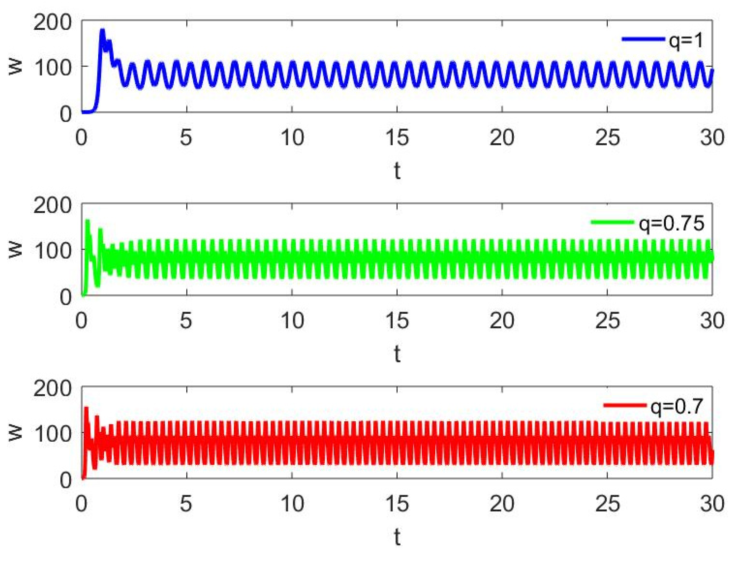
Figure 6 shows the phase diagram between the demand by retailers and the digital production by manufacturers of system (11) with different fractional orders. As shown, when q = 1, $w$ fluctuates more at $x>0$ and less at $x<0$, as the order $q$ decreases to 0.75 and then to 0.7, $w$ fluctuates gradually less at $x>0$ and more at $x<0$. In practice, $x<0$ indicates that the supply of distributors cannot meet the order demand of retailers. The analysis shows that with a small order $q$, then the production of the manufacturers fluctuates more when the supply from the distributors to the retailers is insufficient, while the production of the manufacturers fluctuates less when the supply from the distributors is sufficient. Thus, it indicates that the fractional-order system more accurately reflects the real-world supply chain system compare to the integer-order one.

Figure 7 shows the corresponding time series diagram of the digital production of the manufacturers. As shown in the figure, the smaller the order $q$, the shorter the fluctuation period of the production, indicating that goods are transferred faster at all levels of the supply chain and can meet customer demand faster, resulting in a more stable inventory system and supply chain system.

As shown in Figure 8, the $C_0$ complexity and SE complexity of system (11) are higher when $0.5\le q\le 0.62$, and the values of complexity both oscillate at lower values when $q>0.62$. It shows that the fractional-order system has an order of magnitude higher complexity compared to the integer-order system.

From Figure 4 and Figure 8, we find that the complexity results are consistent with the bifurcation diagrams, indicating that the complexity can reflect the dynamic characteristics of the fractional-order digital manufacturing supply chain system.

4. Synchronization of the Chaotic Fractional-Order Digital Manufacturing Supply Chain System

From the analysis in Section 3, it is understood that the fractional-order digital manufacturing supply chain system is chaotic when the rate at which the digital design of the manufacturer is put into production is low. Without applying appropriate synchronization controllers to the system, the trajectories of the system with different initial values will exhibit different behaviors. In order to achieve synchronization between two supply chain systems with different initial conditions, the controllers can be designed to synchronize the two chaotic systems.

We establish the fractional-order error system by two chaotic fractional-order supply chain systems with different initial conditions, which are called the driving supply chain system and the responding supply chain system, respectively. Let $d=0.7$, then the drive supply chain system is defined as follows

$$\{\begin{array}{l}{D}_t^q{x}_1=y_1-2x_1\\ D_t^q{y}_1=65x_1-x_1{w}_1-y_1\\ D_t^q{z}_1=-0.8z_1+x_1{y}_1\\ D_t^q{w}_1=1.28z_1-3.5w_1\end{array}$$

(12)

And the response supply chain system is given as

$$\{\begin{array}{l}{D}_t^q{x}_2=y_2-2x_2+u_{11}(t)\\ D_t^q{y}_2=65x_2-x_2{w}_2-y_2+u_{12}(t)\\ D_t^q{z}_2=-0.8z_2+x_2{y}_2+u_{13}(t)\\ D_t^q{w}_2=1.28z_2-3.5w_2+u_{14}(t)\end{array}$$

(13)

where $u_{11}(t)$, $u_{12}(t)$, $u_{13}(t)$, $u_{14}(t)$ are the controllers to be determined later.

Denote the error variables as

$$\{\begin{array}{l}{e}_1=x_2-x_1\\ e_2=y_2-y_1\\ e_3=z_2-z_1\\ e_4=w_2-w_1\end{array}$$

(14)

where, $e_1$, $e_2$, $e_3$, $e_4$ denote errors between the drive system and the response system. The fractional-order error system is obtained by subtracting the drive supply chain system from the response supply chain system

$$\{\begin{array}{l}{D}_t^q{e}_1=e_2-2e_1+u_{11}(t)\\ D_t^q{e}_2=65e_1-x_2{w}_2+x_1{w}_1-e_2+u_{12}(t)\\ D_t^q{e}_3=-0.8e_3+x_2{y}_2-x_1{y}_1+u_{13}(t)\\ D_t^q{e}_4=1.28e_3-3.5e_4+u_{14}(t)\end{array}$$

(15)

To synchronize the drive system (12) and the response system (13), suitable controllers are chosen so that the fractional-order error system (15) is asymptotically stable at the origin. In this paper, we consider the controllers as

$$\{\begin{array}{l}{u}_{11}(t)=-e_2\\ u_{12}(t)=-65e_1+x_2{w}_2-x_1{w}_1\\ u_{13}(t)=-x_2{y}_2+x_1{y}_1\\ u_{14}(t)=1.28e_3\end{array}$$

(16)

Then the fractional-order error system (15) becomes

$$\{\begin{array}{l}{D}_t^q{e}_1=-2e_1\\ D_t^q{e}_2=-e_2\\ D_t^q{e}_3=-0.8e_3\\ D_t^q{e}_4=-3.5e_4\end{array}$$

(17)

The fractional-order error system (17) is asymptotically stable based on Lemma 1, which implies that synchronization between (12) and (13) will be realized. This completes the proof.

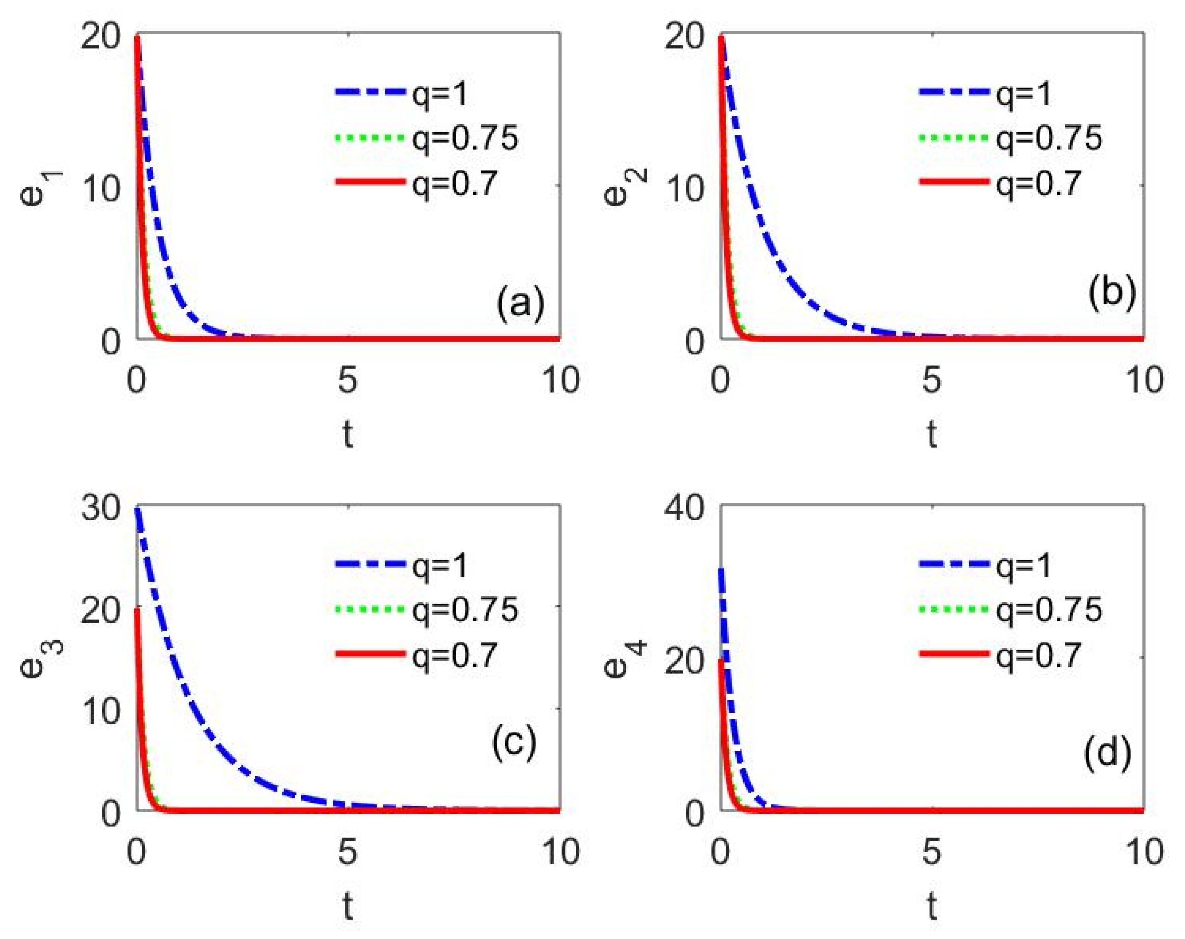
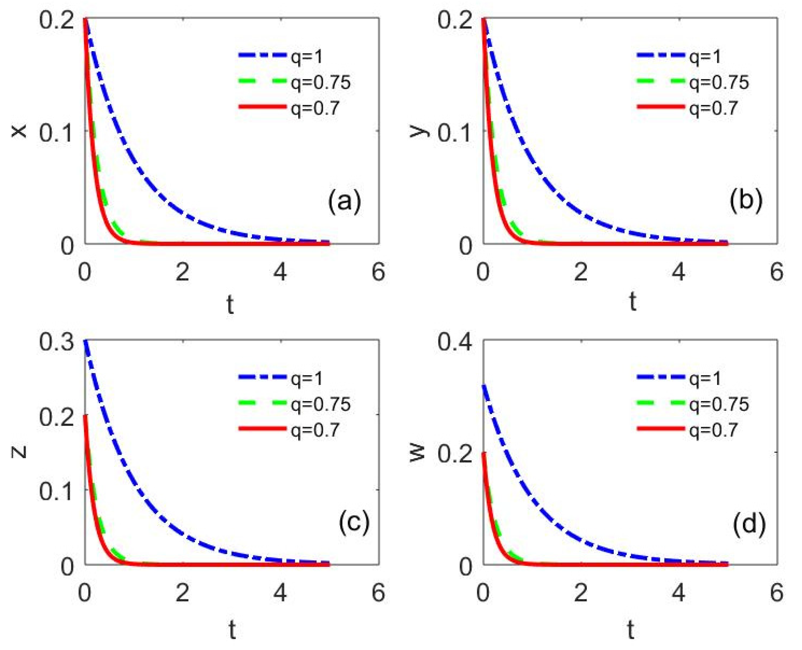
Furthermore, the effect of the fractional orders on the synchronization of two chaotic fractional-order supply chain systems with different initial conditions is studied. Let the parameter $d=0.7$, then both the drive system and the response system are chaotic. Let the initial values of the drive system $(x_{10},y_{10},z_{10},w_{10})=(0.2,0.2,0.3,0.32)$, and the initial values of the response system $(x_{20},y_{20},z_{20},w_{20})=(20,20,30,32)$. The fractional order $q$ is chosen as $q=1$, $q=0.75$, and $q=0.7$, respectively. 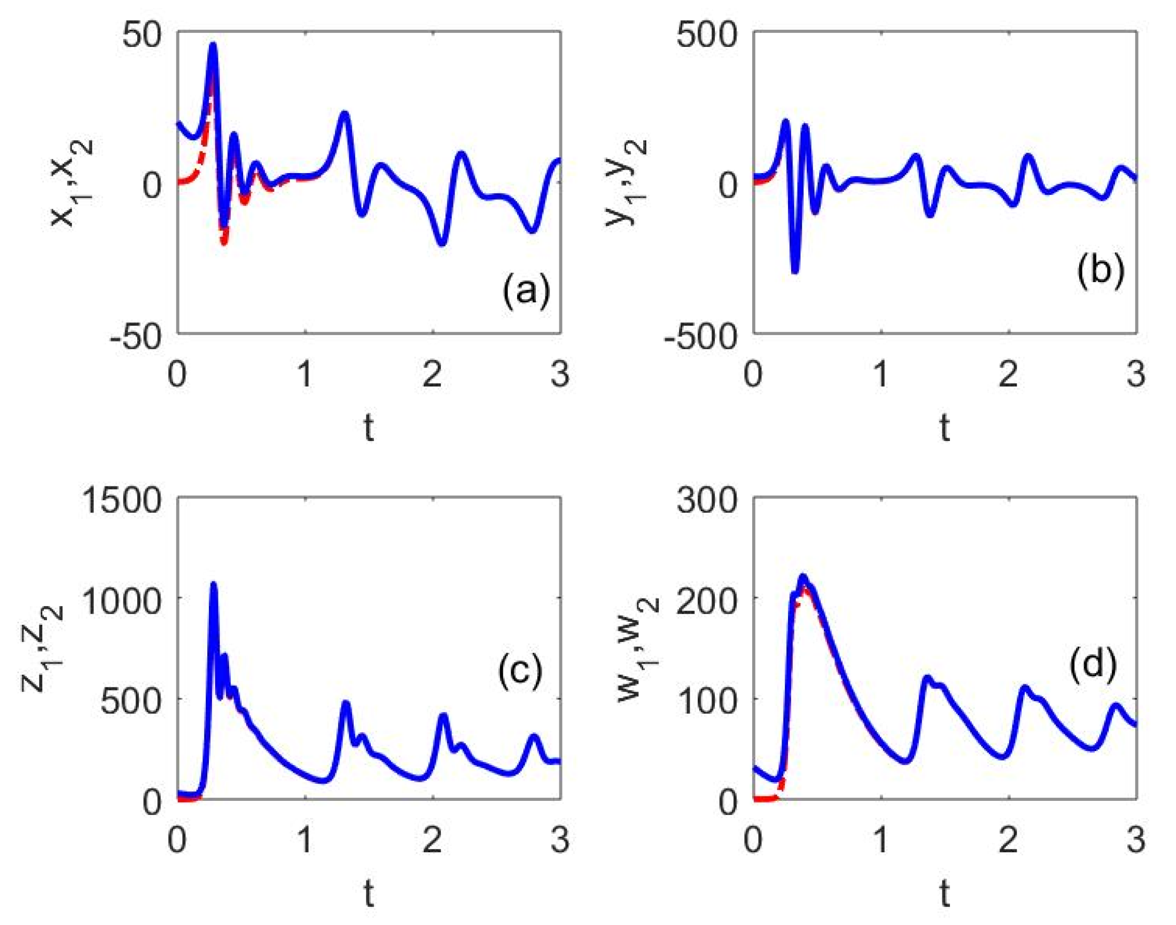The numerical solution of system (17) is obtained by the ADM, and the time series diagrams of system (17) with different fractional orders are shown in Figure 9. As shown in the figure, for two identical fractional-order chaotic supply chain systems (although there are differences in their initial states), the errors gradually converge to zero as time grows. This indicates that the two chaotic systems reach synchronization under the designed controllers, and the smaller the fractional order, the faster the synchronization. This implies that despite the factors such as the bullwhip effect, inventory can be synchronized faster when the order of the fractional-order supply chain systems is decreased, allowing the enterprises to reduce risk more effectively.

In order to see the comparison of the time histories of the drive system and the response system more visually and to further verify the synchronization, the fractional order $q$ is chosen to be 0.75 and the time series of systems (12) and system (13) are plotted in the same figure, as shown in Figure 10. The green line in the figure represents the time series of the drive supply chain system under its initial conditions, and the yellow line represents the time series of the response supply chain system under its initial conditions, and the comparison reveals that the time series of the two systems overlap after $t=1.6$ as time grows. Again, it shows that the designed synchronization controllers are effective and can synchronize the two systems.

5. Control of Fractional-Order Supply Chain Chaotic System

5.1. Equilibrium Point Analysis

The corresponding Jacobian matrix of system (10) is given as follows:

$$J=\left[\begin{array}{cccc}-(n+1+{\theta }_n)& m+{\theta }_m& 0& 0\\ r+{\theta }_r-w& -1& 0& -x\\ y& x& -(d+{\theta }_d)& 0\\ 0& 0& (c+{\theta }_c)(d+{\theta }_d)& -(k-1-{\theta }_k)\end{array}\right]$$

The values of the system parameters are set in Section 2, let $d=0.7$, the equilibrium points can be evaluated by solving the equations $D^{q}x=0$, $D^{q}y=0$, $D^{q}z=0$, and $D^{q}w=0$. System (10) has three equilibrium points, which are, respectively, described as $E_0=\left(0,0,0,0\right),$ $E_1=(-8.3010,-16.6020,172.2656,63.0000),$ $E_2=(8.3010,$ $16.6020,172.2656,63.0000)$. The corresponding eigenvalues are obtained as $E_0$:${\lambda }_1=-3.5$, ${\lambda }_2=-9.5777$, ${\lambda }_3=6.5777$, ${\lambda }_4=-0.8$, $E_1$ and $E_2$:${\lambda }_1=1.1695+3.7637\mathrm{i}$, ${\lambda }_2=1.1695-3.7637\mathrm{i}$, ${\lambda }_3=-4.1018$, ${\lambda }_4=-5.5372$.

From Lemma 1, the equilibrium point $E_0$ is unstable, whereas the stability of $E_1$ and $E_2$ is determined by the value of the fractional order $q$.

5.2. Feedback Controllers

Considering the equilibrium point $E_0$, to control chaos in fractional-order system (10), the feedback controllers $u_{11}(t)$, $u_{12}(t)$, $u_{13}(t)$, $u_{14}(t)$ are considered, then the controlled system is defined as

$$\{\begin{array}{l}{D}_t^{q}x=y-2x+u_{21}(t),\\ D_t^{q}y=65x-xw-y+u_{22}(t),\\ D_t^{q}z=-0.8z+xy+u_{23}(t),\\ D_t^{q}w=1.28z-3.5w+u_{24}(t).\end{array}$$

(18)

For the fractional-order system (10), the following feedback controllers are designed in order to control the system asymptotically stably at the equilibrium point $E_0$(0,0,0,0).

$$\{\begin{array}{l}{u}_{21}(t)=x-y,\\ u_{22}(t)=-65x+xw,\\ u_{23}(t)=-0.2z-xy,\\ u_{24}(t)=-1.28z+2.5w,\end{array}$$

(19)

Then, the controlled system (18) can be written as

$$\{\begin{array}{l}{D}_t^{q}x=-x,\\ D_t^{q}y=-y,\\ D_t^{q}z=-z,\\ D_t^{q}w=-w.\end{array}$$

(20)

The corresponding eigenvalues are ${\lambda }_1={\lambda }_2={\lambda }_3={\lambda }_4=-1$. From Lemma 1, $\left|\arg ({\lambda }_i)\right|>\frac{\pi q}{2}$, then equilibria $E_0$ is asymptotically stable under the chosen controllers as shown in Figure 11.

The simulation result shows the effectiveness of the designed control functions.

The simulation result from Figure 11 shows the effectiveness of the designed control functions. This suggests that the designed controllers can control chaos in fractional-order system (10), and the smaller the fractional order, the faster the system is controlled to the equilibrium point. This implies that when the order of the fractional-order supply chain system is decreased, the system can reach a stable state more quickly.

In the above numerical results from Figure 5, we find that the derivative orders can change the bifurcation types and dynamics of the system. Figure 6 and Figure 7 show that with different orders, supply chain companies have different decisions for inventory and management. Furthermore, Figure 9 indicates that the rate of synchronization is affected by the value of order. Figure 11 also shows that the rate of the system is controlled to the equilibrium point which is affected by the value of fractional order. It again indicates that the derivative order is very important in the fractional-order supply chain chaotic system.

6. Conclusions

In the present research, a fractional-order digital manufacturing supply chain system model was established. Through well-known tools and methods, including the phase portrait, bifurcation diagram, and maximum Lyapunov exponent diagram, the characteristics of the system were explored. The behavior of the system and the effects of the fractional-order derivative on the results of the system were displayed. It was demonstrated that the fractional-order system more accurately reflects the real-world supply chain system compared to the integer-order one. Furthermore, controllers were designed to synchronize two systems with different initial conditions. In addition, the equilibrium point analysis was carried out, and to suppress the chaotic behavior, feedback controllers were designed to stabilize the supply chain system. Our research results can help achieve more stable inventory systems and supply chain systems. In the future, we aim to further study the complexity evolution of fractional-order chaotic supply chain systems. Also, future research can be devoted to the control and synchronization of the proposed model through some more simple controllers with less parameters, such as fractional-order fuzzy controllers, fractional-order PID controllers, and fractional-order ${\mathrm{PI}}^{\lambda }\mathrm{D}$ controllers.

References

1. Mandelbrot, B.B.; Wheeler, J.A. The Fractal Geometry of Nature. Am. J. Phys. 1983, 51, 286–287. [Google Scholar] [CrossRef]
2. He, S.; Sun, K.; Wang, H. Dynamics and synchronization of conformable fractional-order hyperchaotic systems using the Homotopy analysis method. Commun. Nonlinear Sci. Numer. Simul. 2019, 73, 146–164. [Google Scholar] [CrossRef]
3. He, S.; Banerjee, S.; Sun, K. Can derivative determine the dynamics of fractional-order chaotic system? Chaos Solitons Fractals 2018, 115, 14–22. [Google Scholar] [CrossRef]
4. Hu, W.; Ding, D.; Zhang, Y.; Wang, N.; Liang, D. Hopf bifurcation and chaos in a fractional order delayed memristor-based chaotic circuit system. Optik 2017, 130, 189–200. [Google Scholar] [CrossRef]
5. Alidousti, J.; Ghahfarokhi, M.M. Dynamical behavior of a fractional three-species food chain model. Nonlinear Dyn. 2018, 95, 1841–1858. [Google Scholar] [CrossRef]
6. Chen, L.; Yin, H.; Huang, T.; Yuan, L.; Zheng, S.; Yin, L. Chaos in fractional-order discrete neural networks with application to image encryption. Neural Netw. 2020, 125, 174–184. [Google Scholar] [CrossRef] [PubMed]
7. Dulf, E.H.; Vodnar, D.C.; Danku, A.; Muresan, C.I.; Crisan, O. Fractional-order models for biochemical processes. Fractal Fract. 2020, 4, 12. [Google Scholar] [CrossRef] [Green Version]
8. Wang, S.; He, S.; Yousefpour, A.; Jahanshahi, H.; Repnik, R.; Perc, M. Chaos and complexity in a fractional-order financial system with time delays. Chaos Solitons Fractals 2020, 131. [Google Scholar] [CrossRef]
9. Zhang, Z.; Zhang, J.; Cheng, F.; Liu, F.; Ding, C. Dynamic analysis of a novel time-lag four-dimensional fractional-order fi-nancial system. Asian J. Control 2021, 23, 536–547. [Google Scholar] [CrossRef]
10. Yuan, L.; Yang, Q. Parameter identification and synchronization of fractional-order chaotic systems. Commun. Nonlinear Sci. Numer. Simul. 2012, 17, 305–316. [Google Scholar] [CrossRef]
11. Yuan, L.; Zheng, S.; Alam, Z. Dynamics analysis and cryptographic application of fractional logistic map. Nonlinear Dyn. 2019, 96, 615–636. [Google Scholar] [CrossRef]
12. Azar, A.T.; Vaidyanathan, S. Chaos Modeling and Control Systems Design; Springer International Publishing: Berlin/Heidelberg, Germany, 2015; Volume 581. [Google Scholar]
13. Zheng, S. Stability of uncertain impulsive complex-variable chaotic systems with time-varying delays. ISA Trans. 2015, 58, 20–26. [Google Scholar] [CrossRef] [PubMed]
14. Zheng, S. Synchronization analysis of time delay complex-variable chaotic systems with discontinuous coupling. J. Frankl. Inst. 2016, 353, 1460–1477. [Google Scholar] [CrossRef]
15. Harshavarthini, S.; Sakthivel, R.; Ma, Y.-K.; Muslim, M. Finite-time resilient fault-tolerant investment policy scheme for chaotic nonlinear finance system. Chaos Solitons Fractals 2019, 132, 109567. [Google Scholar] [CrossRef]
16. Cao, Y. Chaotic synchronization based on fractional order calculus financial system. Chaos Solitons Fractals 2019, 130, 109410. [Google Scholar] [CrossRef]
17. Al-khedhairi, A. Dynamical analysis and chaos synchronization of a fractional order novel financial model based on Ca-puto-Fabrizio derivative. Eur. Phys. J. Plus 2019, 134, 532. [Google Scholar] [CrossRef]
18. Ma, J.; Ren, W.; Zhan, X. Study on the Inherent Complex Features and Chaos Control of IS–LM Fractional-Order Systems. Entropy 2016, 18, 332. [Google Scholar] [CrossRef] [Green Version]
19. Dousseh, P.Y.; Ainamon, C.; Miwadinou, C.H.; Monwanou, A.V.; Orou, J.B.C. Chaos in a financial system with fractional order and its control via sliding mode. Complexity 2021, 2021, 4636658. [Google Scholar] [CrossRef]
20. Suribabu, G.; Chiranjeevi, T. Implementation of Fractional Order PID Controller for an AVR System Using GA and ACO Optimization Techniques. IFAC-PapersOnLine 2016, 49, 456–461. [Google Scholar] [CrossRef]
21. Jakovljević, B.; Lino, P.; Maione, G. Control of double-loop permanent magnet synchronous motor drives by optimized frac-tional and distributed-order PID controllers. Eur. J. Control. 2021, 58, 232–244. [Google Scholar] [CrossRef]
22. Xin, Y.; Zheng, A.; Hu, W. Adequate analysis of a reliability model for a supply chain system. Math. Pract. Underst. 2008, 1, 46–52. [Google Scholar]
23. Peng, Y.; Wu, J.; Wen, S.; Feng, Y.; Tu, Z.; Zou, L. A New Supply Chain System and Its Impulsive Synchronization. Complexity 2020, 2020, 2414927. [Google Scholar] [CrossRef]
24. Wang, W.; Ren, L.; Fu, W.; Yu, X.; Hao, L. Complex dynamical behavior of supply chain systems. Mech. Sci. Technol. 2011, 30, 302–308. [Google Scholar]
25. Dong, H.; Xu, D. Research on chaotic control of closed-loop supply chain under three-channel recycling model. Complex Syst. Complex. Sci. 2020, 17, 55–61. [Google Scholar]
26. Yibulayin, G.; Guo, W.; Abdulgehman, K.; Yu, K. Chaotic dynamics of multi-channel supply price game between specialty retailers and factory direct sellers. Oper. Res. Manag. 2019, 28, 54–59. [Google Scholar]
27. Yu, S.; Chen, G. Simulation study of supply chain model dynamics from the perspective of complex systems. Comput. Simul. 2016, 33, 328–331. [Google Scholar]
28. Wang, G.; Ma, J.; Xin, B. Construction of supply chain yield game model and complexity simulation analysis. Comput. Eng. Appl. 2011, 47, 22–25. [Google Scholar]
29. Forrester, J.W. Industrial Dynamics. J. Oper. Res. Soc. 1997, 48, 1037–1041. [Google Scholar] [CrossRef]
30. Göksu, A.; Kocamaz, U.E.; Uyaroğlu, Y. Synchronization and control of chaos in supply chain management. Comput. Ind. Eng. 2015, 86, 107–115. [Google Scholar] [CrossRef]
31. Gao, F.; Cao, W. Dynamics analysis of a three-dimensional supply chain fractional-order difference game model. Comput. Eng. Appl. 2018, 54, 246–252. [Google Scholar]
32. Yan, L.; Liu, J.; Xu, F.; Teo, K.L.; Lai, M. Control and synchronization of hyperchaos in digital manufacturing supply chain. Appl. Math. Comput. 2020, 391, 125646. [Google Scholar] [CrossRef]
33. Podlubny, I. Fractional Differential Equations, Vol. 198 of Mathematics in Science and Engineering; Academic Press: San Diego, CA, USA, 1999. [Google Scholar]
34. Tavazoei, M.S.; Haeri, M. Chaotic attractors in incommensurate fractional order systems. Phys. D Nonlinear Phenom. 2008, 237, 2628–2637. [Google Scholar] [CrossRef]
35. Charef, A.; Sun, H.; Tsao, Y.; Onaral, B. Fractal system as represented by singularity function. IEEE Trans. Autom. Control 1992, 37, 1465–1470. [Google Scholar] [CrossRef]
36. Sun, H.; Abdelwahab, A.; Onaral, B. Linear approximation of transfer function with a pole of fractional power. IEEE Trans. Autom. Control 1984, 29, 441–444. [Google Scholar] [CrossRef]
37. He, S.; Sun, K.; Peng, Y. Detecting chaos in fractional-order nonlinear systems using the smaller alignment index. Phys. Lett. A 2019, 383, 2267–2271. [Google Scholar] [CrossRef]
38. He, S.; Sun, K.; Wang, H. Adomian decomposition of fractional order chaotic systems solution and its complexity analysis. J. Phys. 2014, 63, 58–65. [Google Scholar]
39. Staniczenko, P.P.A.; Lee, C.F.; Jones, N.S. Rapidly detecting disorder in rhythmic biological signals: A spectral entropy measure to identify cardiac arrhythmias. Phys. Rev. E 2009, 79, 011915. [Google Scholar] [CrossRef] [PubMed]
40. Shen, E.; Cai, Z.; Gu, F. Mathematical foundation of a new complexity measure. Appl. Math. Mech. 2005, 26, 1188–1196. [Google Scholar]
Figure 1. Bifurcation diagram of system (11).
Fractalfract 05 00128 g001
Figure 2. Maximum Lyapunov exponent of system (11).
Fractalfract 05 00128 g002
Figure 3. Phase portraits projected onto the x w phase plane of system (18) when q = 0.75 . (a) d = 0.7 . (b) d = 2.9 . (c) d = 3.5 . (d) d = 4 .
Fractalfract 05 00128 g003
Figure 4. C 0 and SE complexity.
Fractalfract 05 00128 g004
Figure 5. Bifurcation diagram of system (11) with q.
Fractalfract 05 00128 g005
Figure 6. Phase portrait projected onto the xw phase plane of system (11) with the order q = 1 , q = 0.75 , and q = 0.7 when d = 3.5 .
Fractalfract 05 00128 g006
Figure 7. Time series of system (11) with the order q = 1 , q = 0.75 , and q = 0.7 when d = 3 .
Fractalfract 05 00128 g007
Figure 8. C 0 and SE complexity with the order q varying from 0.5 to 1 when d = 3 .
Fractalfract 05 00128 g008
Figure 9. Time series of error system (17) with the order q = 1 , q = 0.75 , and q = 0.7 .
Fractalfract 05 00128 g009
Figure 10. Time series of the drive supply chain system (12) (blue line) and the response supply chain system (13) (red dot line) when q = 0.75 , and d = 0.7.
Fractalfract 05 00128 g010
Figure 11. Time series of the controlled system (18) with the order q = 1 , q = 0.75 , and q = 0.7 .
Fractalfract 05 00128 g011
Publisher’s Note: MDPI stays neutral with regard to jurisdictional claims in published maps and institutional affiliations.