Demand Response Optimal Dispatch and Control of TCL and PEV Agents with Renewable Energies

Abstract

Demand response (DR) flexible loads can provide fast regulation and ancillary services as reserve capacity in power systems. This paper proposes a demand response optimization dispatch control strategy for flexible thermostatically controlled loads (TCLs) and plug-in electric vehicles (PEVs) with stochastic renewable power injection. Firstly, a chance constraint look-ahead programming model is proposed to maximize the social welfare of both units and load agents, through which the optimal power scheduling for TCL/PEV agents can be obtained. Secondly, two demand response control algorithms for TCLs and PEVs are proposed, respectively, based on the aggregate control models of the load agents. The TCLs are controlled by its temperature setpoints and PEVs are controlled by its charging power such that the DR control objective can be fulfilled. It has been shown that the proposed dispatch and control strategy can coordinate the flexible load agents and the renewable power injection. Finally, the simulation results on a modified IEEE 39 bus system demonstrate the effectiveness of the proposed demand response strategy.

1. Introduction

With the rapid increase in energy consumption and environmental pollution, renewable energy power generation is becoming more and more popular and various kinds of distributed generations are connecting into the power grid. Meanwhile, the incorporation of renewable energy units gives rise to the increasing need for resource capacity or ancillary services if there exists major forecast uncertainty. Meanwhile, flexible loads in the demand side can provide different kinds of ancillary services, such as frequency regulation, load following, and other services. The widely adopted flexible loads for these services include thermostatically controlled loads (TCLs) and plug-in electric vehicles (PEVs), which can respond the power dispatch or electricity price timely. To address these concerns, there have been several valuable studies on the coordination and interaction of traditional units, renewable units, and flexible loads of source–load systems [1,2,3,4].

Renewable power generation has gained much attention and been in an increasing trend, which is beneficial to environment and economics. Especially, wind and photovoltaic generation are thought to be the most developed renewable sources worldwide. However, the power produced by these renewable energies largely depends on natural environmental conditions, such as wind speed or illumination intensity, which are stochastic and cannot be precisely predicted.

The uncertainty of renewable power may pose new challenges for power system operation and control, especially during times of high penetration [5]. To provide a flexible and comprehensive consideration of the forecast error of renewable power [6], a common solution is to restrict wind power and abandon light power so as to protect the power systems. Another solution is utilizing the various optimization methods. The look-ahead dispatch method was considered in [7,8], which has proved to be an effective strategy to reduce the power imbalance caused by the injection of renewable power [9]. By taking into account the uncertainty of renewable power, robust optimization [10,11], stochastic optimization [12,13], and chance-constrained stochastic optimization [14,15] have been the most popular methods to account for uncertainties in power generation.

On the other hand, the demand response of power grids has already switched from traditional mode of load curtailment to the mode of dynamical response without interfering with users’ comfort levels [16]. DR optimization has received much attention. The authors in [17] proposed a hierarchical demand response architecture to control and coordinate the performance of various DR category resources. Demand response controllability was investigated in [18] for the unit commitment model with limited predictability and residential DR resources. By considering the site selection and the incentive price, an optimal strategy for responsive loads was proposed in [19] for source–network–load system. Online demand response for nondeferrable loads was investigated in [20] with rechargeable battery and renewable energy. By the method of the alternating direction method of multipliers, a hierarchical robust distributed optimization was proposed for demand response services [21].

As for the TCL agents, it has been shown that TCLs can provide power-balancing reserves when aggregated due to their thermal energy storage capacity [22,23]. The authors in [24] demonstrated that TCLs can be considered as rapid DR activation loads for power system control operations. By using switching-rate actuation, the authors in [25] studied the demand response of TCLs and household refrigerators. Distributed load following was investigated in [16] for aggregate TCL loads. The authors in [26] presented a mean-field model for analysis and control of the aggregate demand of heterogeneous TCLs. By using a stochastic Markov decision process and distributed robust optimization, ref. [27] internalized the exogenous uncertain dynamics of TCLs.

Literature on demand response and EV charging scheduling has proved that EVs will become the main demand response resource in the near-future. Many researches have concentrated on charging optimization and control problems. The authors in [28,29,30] investigated the optimal energy management and control problems of smart home with PEVs and photovoltaic arrays. By designing a smart-charging scheme for PEV, it was shown in [31] that the aggregate EVs are able to reduce the peak demand or peak shaving. A fair demand response strategy for EVs was proposed in [32] for a cloud-based energy management service in a given time period. The authors in [33] proposed a charging load model for an electric vehicle charging station, which could be integrated to distribution systems so as to obtain the optimal charging decisions for demand response provision.

Both aggregate TCLs and aggregate PEVs are large-scale flexible loads in power grids, which can be involved in the DR program together to share the power imbalance. By considering the uncertainty in renewable energy generation, load consumption, and load reserve capacities, a chance-constrained optimal power flow model was proposed in [34,35] to procure minimum cost energy. The authors in [36] proposed a chance-constrained optimal power flow model to schedule the power production of both generators and controllable electric loads. By the method of stochastic model predictive control, the authors in [37] investigated the optimal power dispatch and control for power grids with renewable energy resources and EVs. Based on the mixed-integer linear programming method, intelligent DR for industrial energy management was designed in [38] by considering TCLs and EVs.

Despite there being several related studies conducted for TCLs and PEVs, there are still some challenging problems that remain unsolved. According to different DR incentive strategies, such as price response, policy response, or control response, the actual customers’ responses are varied and diverse. As for the control response loads, the basic control model of the objective is needed. The individual models of the TCL and PEV are mature while the aggregate models and the aggregate control strategies of these loads are immature. Motivated by the above observations, this paper intends to investigate the optimization dispatch and demand response control of source–load systems with uncertain renewable power injection and flexible TCL and PEV load agents. To the best knowledge of the authors, most of the demand response problems are solved by various kinds of optimization models and methods; few published literature have investigated this problem by aggregate control algorithms. This paper aims to fill this gap and solve the demand response optimal power allocation and response problems of source–load systems via aggregate control models and strategies for flexible loads.

The main contributions are summarized three-fold: (1) A probabilistic controllable interval is introduced to the chance-constrained look-ahead optimization, which can cope with the uncertainty of both the renewable power generation and the flexible load response; (2) compared with discrete-time on/off control of TCLs, a continuous-time setpoint temperature regulating control algorithm based on aggregated models is proposed to guidance the power change of the TCL agent; (3) a time-varying charging power control algorithm based on the saturation function is proposed for the PEV agent such that the aggregate PEVs can follow the reference power trajectory.

An outline of the remainder of the paper is organized as follows. Section 2 states the problem formulation and the optimization and control framework. Section 3 provides the chance-constrained look-ahead programming model for the source–load system with the injection of renewable power and flexible TCL/PEV agents. Section 4 describes the aggregate model for TCL/PEV agents and designs the corresponding control algorithms for the optimal power profile tracking. Section 5 shows the effectiveness of the proposed optimization and control algorithm on a modified IEEE 39 bus system. Section 6 discusses the optimization and control framework and draws the conclusions.

Some abbreviations are provided in the following before the main results.

Acronyms	Full Name
DR	Demand response
TCL	Thermostatically controlled load
TCL	Plug-in electric vehicle
SAA	Sample average approximation
TOU	Time-of-use
SoC	State-of-charge

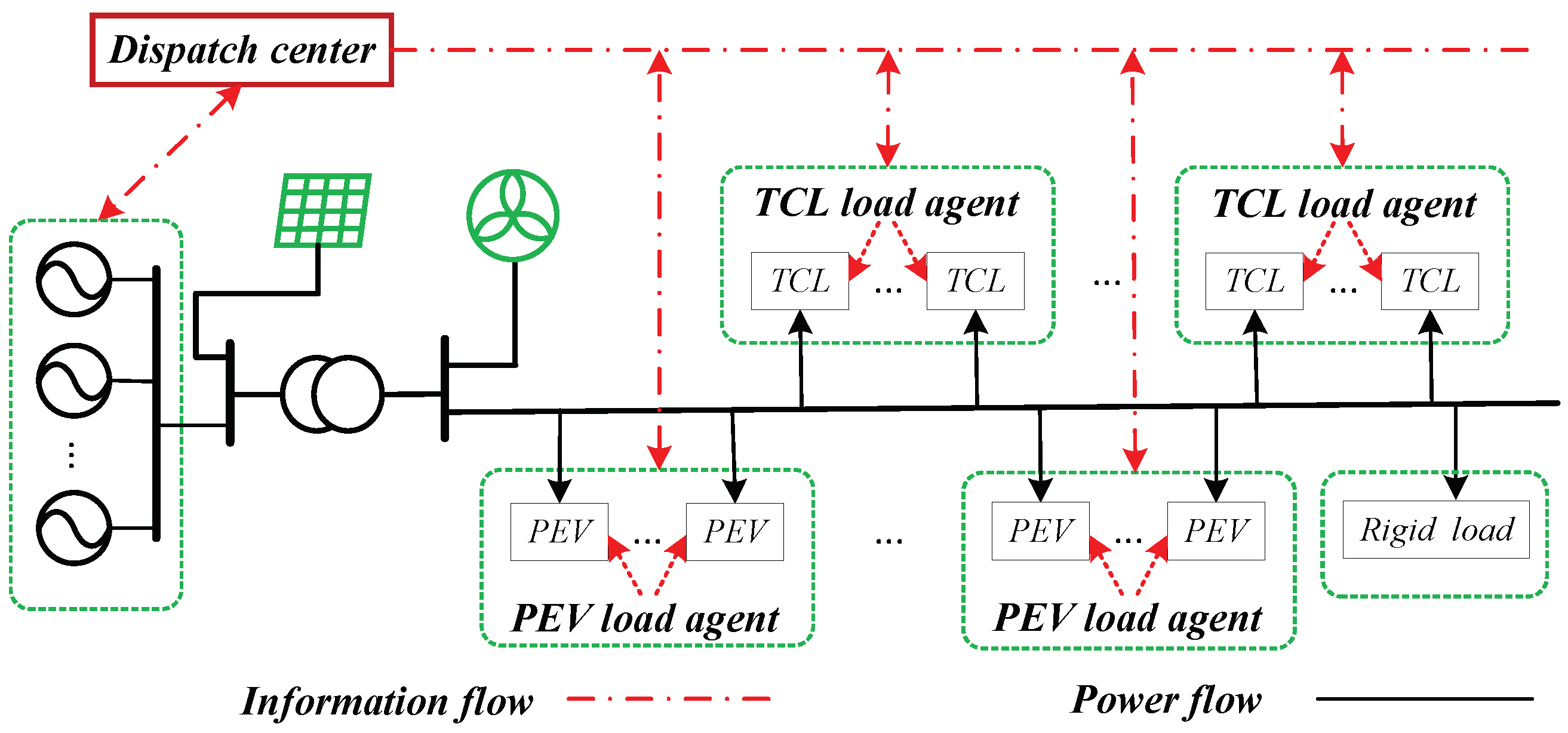
2. Problem Formulation

Consider the coordination optimization problem of a source–load system, where the source of the system includes the traditional generating units and renewable power (mainly wind power and photovoltaic power) and the load of the system includes rigid load and flexible load. The rigid loads, such as lighting and computers, are always uncontrollable but can be predicted. The flexible loads, such as thermostatically controlled loads and plug-in electric vehicles, can be controlled by the corresponding control signals. On the other hand, the renewable power injection is always a random variable because the wind speed and the ambient temperature and illumination are always random. Therefore, how to balance the power production and consumption with the maximal social welfare is a crucial problem among units and flexible loads.

This paper intends to solve this problem by setting up a chance-constrained look-ahead programming model for the source–load system and designing two kinds of demand response control algorithms for TCLs and EVs. Specifically, flexible loads are aggregated as a load agent, which can be involved in the electricity market to participate in the load bidding. The terminal DR loads are controlled by the load agent by issuing the corresponding control signals. The schematic diagram of the optimization dispatch is shown in Figure 1.

Based on the prediction of the rigid load, the actual renewable power injection, and the day-ahead power generation plan, the look-ahead optimization dispatch with chance constraints can be solved by the sample average approximation (SAA) method [39,40]. Furthermore, the generating units respond with optimal generating instructions and the flexible load agents achieve the optimal power profile by demand response control of massive-terminal, small, controlled loads. The detailed control models and the control algorithms of TCL agents and PEV agents will be discussed in the following section.

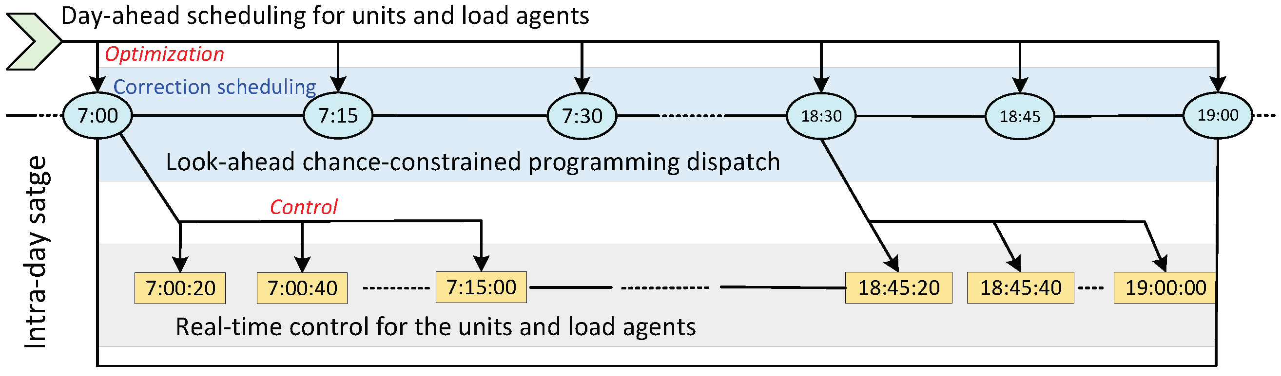
3. Chance-Constrained Look-Ahead Optimization

This paper considers the joint real-time economic dispatch problem for generating units and flexible load agents by considering the uncertainty of renewable energy power generation. The objective of the power scheduling is to maximize social welfare, i.e., maximizing both generating units and load agents:

$$\begin{array}{c}\hfill max\sum _{t=1}^T\mathbb{F}\left(\mathcal{P}\left(t\right)\right)=\sum _{t=1}^T\left[\sum _{i\in G}{\mathsf{\Omega }}_{G,i}\left(P_{G,i}\left(t\right),p\left(t\right)\right)+\sum _{j\in L}{\mathsf{\Omega }}_{L,j}\left(P_{L,j}\left(t\right),p\left(t\right)\right)\right],\end{array}$$

(1)

where $\mathbb{F}$ is the total social welfare with respect to the real-time power variable $\mathcal{P}\left(t\right)={[P_1\left(t\right),P_2\left(t\right),\dots ,P_{\left|G\right|+\left|L\right|}\left(t\right)]}^T={\mathcal{P}}_0\left(t\right)+\Delta \mathcal{P}\left(t\right)$ (day-ahead scheduling plus intraday corrective scheduling); $p\left(t\right)$ is the time-of-use (TOU) power price; ${\mathsf{\Omega }}_{G,i}(·)$ and ${\mathsf{\Omega }}_{L,j}(·)$ are the welfare functions of the ith generating unit and the jth load agent, which are given as follows:

$$\begin{array}{cc}\hfill & {\mathsf{\Omega }}_{G,i}(P_{G,i}\left(t\right),p\left(t\right))=p\left(t\right)P_{G,i}\left(t\right)-C_i\left(P_{G,i}\left(t\right)\right),\hfill \\ & {\mathsf{\Omega }}_{L,j}(P_{L,j}\left(t\right),p\left(t\right))=U_l\left(P_{L,j}\left(t\right)\right)-p\left(t\right)P_{L,j}\left(t\right).\hfill \end{array}$$

(2)

For the units, the cost function $C_i(·)$ usually can be approximated by a quadratic convex function $C_i\left(P_i\right)=a_i{P}_i^2+b_i{P}_i+c_i$, where $a_i$, $b_i$, and $c_i$ are predetermined constants and $P_i$ is the generated power. For the load agents, the utility function $U_j(·)$, often assumed to be the convex utility function with the zero initial value, is a quadratic utility function that can be described by [41,42]

$$U_j\left(P_{L,j}\right)=\{\begin{array}{c}{\omega }_j{P}_{L,j}-{\alpha }_j{P}_{L,j}^2,0\le P_{L,j}\le \frac{{\omega }_j}{2{\alpha }_j},\hfill \\ {\omega }_j^2/4{\alpha }_j,P_{L,j}\ge \frac{{\omega }_j}{2{\alpha }_j},\hfill \end{array}$$

(3)

where ${\omega }_j$ and ${\alpha }_j$ are predetermined constant coefficients.

Considering the randomness of the actual renewable power, the following chance constraint with a controllable interval is involved:

$$\begin{array}{c}\hfill \mathrm{Pr}\left(P_{lo}\le \sum _{i\in G}{P}_{G,i}\left(t\right)+P_{Rew}\left(t\right)-\sum _{j\in L}{P}_{L,j}\left(t\right)-P_D\left(t\right)\le P_{hi}\right)\ge p_a,\end{array}$$

(4)

where $[P_{lo},P_{hi}]$ is the controllable confidence interval of the source–load system, which is often set to be smaller than the actual operation interval because of the response uncertainty of the flexible DR loads; $P_{Rew}\left(t\right)=P_{wi}\left(t\right)+P_{pv}\left(t\right)$ is the renewable power injection with the random wind power variable $P_{wi}$ and the random photovoltaic power $P_{pv}$; $P_D$ is the prediction value of the rigid load in the system; the probability $p_a$ is required to be at least $95\%$.

Other considered inequality constraint conditions for such an optimization problem are given as follows:

$$\{\begin{array}{c}{P}_{G,i}^{min}\le P_{G,i}\left(t\right)\le P_{G,i}^{max},\hfill \\ -R_{G,i}^{\mathrm{dn}}\le \frac{1}{\Delta T}\left(P_{G,i}(t+1)-P_{G,i}\left(t\right)\right)\le R_{G,i}^{\mathrm{up}},\hfill \\ P_{L,j}^{min}\left(t\right)\le P_{L,j}\left(t\right)\le P_{L,j}^{max}\left(t\right),\hfill \\ -R_{L,j}^{\mathrm{dn}}\le \frac{1}{\Delta T}\left(P_{L,j}(t+1)-P_{L,j}\left(t\right)\right)\le R_{L,j}^{\mathrm{up}},\hfill \end{array}$$

(5)

for $\forall i\in G,j\in L$, and $t=1,\dots ,T$; $P_{G,i}^{min}$ and $P_{G,i}^{max}$ are the lower and upper bounds for ith generating unit; $P_{L,j}^{min}\left(t\right)$ and $P_{L,j}^{max}\left(t\right)$ are the time-varying lower and upper bounds for jth load agent; $R_{G/L}^{\mathrm{dn}}$ and $R_{G/L}^{\mathrm{up}}$ are the lower and upper ramping rates of the units and load agents.

By the sample average approximation method [39,40], the optimal power scheduling for units and flexible load agents can be obtained by solving the look-ahead optimization (1)–(5) with chance constraint. In the following, the design of the demand response control algorithms for the aggregate TCL agents and PEV agents will be provided.

Remark 1.

The power variability and uncertainty of the renewable power are handled by the probabilistic chance-constrained optimization, where the probability distributions of the wind power and the PV power are assumed to be mutually independent. Then, the joint probability density function can be derived by the probability theory. Then, the sample of the renewable power can be generated by its probability distribution. The power balance constraint is transformed to be a probability confidence interval with a predefined confidence level $p_a$, which is able to cope with the volatility of the renewable power. On the other hand, the inherent uncertainty of flexible TCLs and PEVs is absorbed by the reserve capacity of the system, i.e., the controllable confidence interval of the optimization constraint (4) can be set smaller than the actual operation interval of the source–load system.

4. Demand Response Control of Load Agents

It is well-known that both TCLs and PEVs are small loads in the distribution grid compared with the traditional generating units in the main grid. Therefore, how to control these dispersive and numerous small loads to fulfill a global optimization and control objective is a key problem in the implementation of the DR control. The aggregate approximate models are critical for such an optimization and control realization, which will simplify the complex task for the decentralized control strategies. In the actual control process, one needs to design the corresponding control strategies such that the aggregate power $P_T\left(t\right)$ of all terminal-controllable loads can track the reference power trajectory $P_{ref}\left(t\right)$ optimized in the chance-constrained optimization. The approximate models for aggregated TCLs and PEVs are utilized in this paper, based on which the error feedback control strategies are proposed. The following provides detailed models and control algorithms.

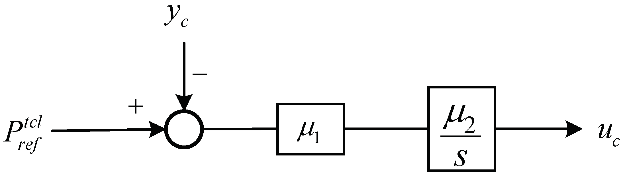
4.1. Aggregated TCL Model and Feedback Control

Suppose a population of homogeneous TCLs under a common control area is aggregated as a TCL agent, the aggregate power of which—based on the temperature control—is approximated by a bilinear system [43] as follows:

$$\{\begin{array}{c}{\dot{x}}_c\left(t\right)=A_c{x}_c\left(t\right)+B_c{x}_c\left(t\right)u_c\left(t\right),\hfill \\ y_c\left(t\right)=C_c{x}_c\left(t\right),\hfill \end{array}$$

(6)

where $x_c\left(t\right)\in {\mathbb{R}}^Q$ is the internal state denoting the average number of off or on TCLs in each temperature subinterval of the temperature deadband; $P_T\left(t\right)=y_c\left(t\right)\in \mathbb{R}$ is the approximate aggregate power output of the TCL agent; the coefficient matrices $A_c,B_c,C_c$ can be found in [43], which are omitted here due to space limits; $u_c\left(t\right)\in \mathbb{R}$ is an incorporated control input satisfying the constraint

$$\begin{array}{c}\hfill u_c\left(t\right)=\frac{1}{CR}(\Delta {\theta }_a\left(t\right)-\Delta {\theta }_{set}\left(t\right))-\Delta {\dot{\theta }}_{set}\left(t\right),\end{array}$$

(7)

where C (kWh/${}^{\circ }$C) is the thermal capacitance and R (${}^{\circ }$C/kW) is the thermal resistance; $\Delta {\theta }_a\left(t\right)={\theta }_a\left(t\right)-{\theta }_{base}$ is the deviation value between the ambient temperature ${\theta }_a\left(t\right)$ and the base value ${\theta }_{base}$; $\Delta {\theta }_{set}\left(t\right)={\theta }_{set}\left(t\right)-{\theta }_{set}^{des}$ is a bounded deviation value between the actual temperature setpoint ${\theta }_{set}\left(t\right)$ and preferred setpoint temperature ${\theta }_{set}^{des}$ for the comfort levels of customers. $\Delta {\dot{\theta }}_{set}$ is the changing rate of the setpoint temperature ${\theta }_{set}\left(t\right)$, which needs to be designed within an interval $[{\overline{\alpha }}_{on},{\overline{\alpha }}_{off}]$ so as to make the aggregate bilinear model (6) make sense, see the detailed illustration in [44].

Parameters ${\overline{\alpha }}_{on}$ and ${\overline{\alpha }}_{off}$ are functions with the independent variables ${\theta }_{base}$ and ${\theta }_{set}^{des}$, given as

$$\{\begin{array}{c}{\overline{\alpha }}_{on}({\theta }_{base},{\theta }_{set}^{des})=\frac{1}{CR}({\theta }_{base}-{\theta }_{set}^{des}-R{P}_r),\hfill \\ {\overline{\alpha }}_{off}({\theta }_{base},{\theta }_{set}^{des})=\frac{1}{CR}({\theta }_{base}-{\theta }_{set}^{des}),\hfill \end{array}$$

where $P_r$ (kW) is the energy transfer rate to or from the thermal mass, which is positive for cooling TCLs.

Next, the setpoint temperature ${\theta }_{set}\left(t\right)$ is determined indirectly by viewing the incorporated control $u_c\left(t\right)$ as an entire variable. By the optimization calculation from the dispatch center, the optimal power profile $P_{ref}^{tcl}\left(t\right)$ for the TCL agent can be derived. The updating of control input $u_c\left(t\right)$ is proposed based on the error feedback control:

$$\begin{array}{c}\hfill u_c\left(t\right)={\mu }_1\left(P_{ref}^{tcl}\left(t\right)-y_c\left(t\right)\right)+{\mu }_2{\int }_{t_0}^t\left(P_{ref}^{tcl}\left(t\right)-y_c\left(t\right)\right)\mathrm{d}t,\end{array}$$

(8)

where ${\mu }_1$ and ${\mu }_2$ are the control gains. The control structure is given in Figure 2.

While the actual temperature setpoint deviation values of TCLs can be updated by substituting (8) into (7). Furthermore, the real-time setpoint temperature ${\theta }_{set}\left(t\right)$ for the TCLs in the load agent can be obtained by

$$\begin{array}{c}\hfill {\theta }_{set}\left(t\right)={\theta }_{set}^{des}+\Delta {\theta }_{set}\left(t\right).\end{array}$$

(9)

According to the generated setpoint temperature control signal, the temperature of each TCL changes by the following temperature regulation differential equation:

$$\begin{array}{c}\hfill \frac{\mathrm{d}\theta \left(t\right)}{\mathrm{d}t}=\frac{1}{CR}\left({\theta }_a\left(t\right)-\theta \left(t\right)-s\left(t\right)R{P}_r\right),\end{array}$$

(10)

where $\theta \left(t\right)$ is the internal temperature of the conditioned mass. The operation state $s\left(t\right)$ is governed by the following thermostatic switching law:

$$\begin{array}{c}\hfill s\left(t\right)=\left\{\begin{array}{cc}0,& \mathrm{if}s(t-\tau )=1\&\theta \left(t\right)<{\theta }^{-}\left(t\right)\\ 1,& \mathrm{if}s(t-\tau )=0\&\theta \left(t\right)>{\theta }^{+}\left(t\right)\\ s(t-\tau ),& \mathrm{otherwise}\end{array}\right.\end{array}$$

(11)

where $\tau$ is the sampling period of temperature, and the lower and upper boundaries of the temperature deadband are given as

$$\begin{array}{c}\hfill {\theta }^{-}\left(t\right)={\theta }_{set}\left(t\right)-\frac{{\delta }_{db}}{2};{\theta }^{+}\left(t\right)={\theta }_{set}\left(t\right)+\frac{{\delta }_{db}}{2}.\end{array}$$

(12)

The deadband of each controlled TCL is a time-varying interval $[{\theta }^{-}\left(t\right),{\theta }^{+}\left(t\right)]$, since the setpoint temperature is regulated according to the global optimization objective.

In the above aggregate model (6), the parameters of TCLs are assumed to be homogeneous for model simplification. As for the heterogeneous TCLs, there are two methods to approximate the aggregate power. The first one is to utilize the averaged equivalent model with the averaged equipment parameters. The second one is to divide the heterogeneous TCLs to multiple homogeneous groups and model the homogeneous TCLs by an aggregate model.

4.2. Aggregated PEV Model and Feedback Control

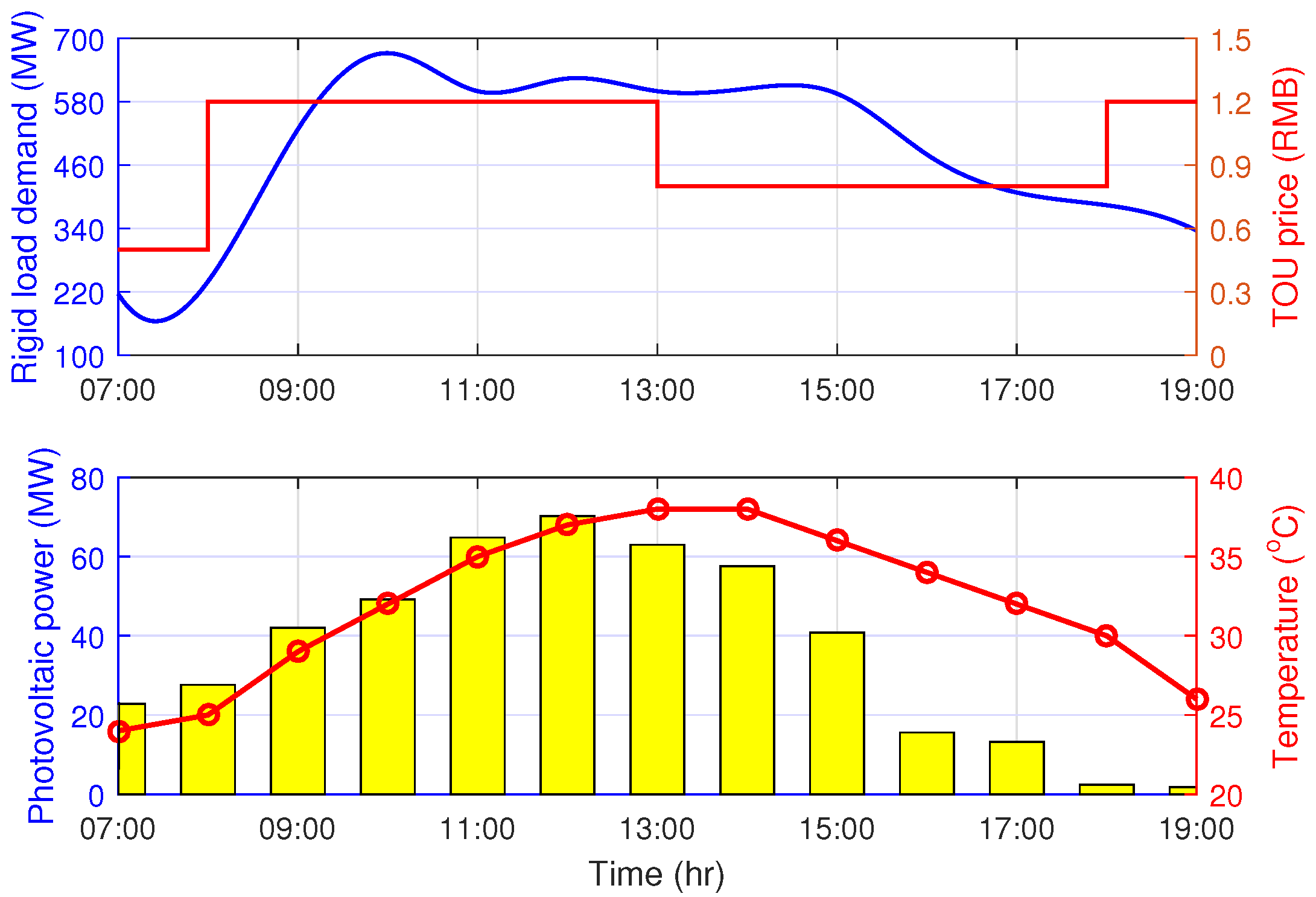
As for the PEV in the power grid, the SoC equation of a single PEV is always utilized to characterize the process of power consumption:

$$\begin{array}{c}\hfill SoC(k+1)=SoC\left(k\right)+\frac{{\eta }_e}{B_e}{u}_e\left(k\right)P_e^{max}\Delta t,\end{array}$$

(13)

where $B_e$ denotes the battery capacity; ${\eta }_e$ is the charging efficiency; $P_e^{max}$ is the maximal charging power of the PEV; $\Delta t$ is the sampling period of the SoC value; $u_e\left(k\right)$ is the charging ratio that needed to be designed. The value of SoC is distributed in the interval $[0,1]$, often characterized by an actual interval $[So{C}_{min},So{C}_{max}]$, where $So{C}_{min}$ is the minimal value for the charging battery and $So{C}_{max}$ is the objective charging state.

Suppose a population of PEVs under a common charging control area is aggregated as a PEV agent, and the aggregate charging control model of the agent is given by a transport-based load model [45]:

$$\{\begin{array}{c}{\dot{x}}_e\left(t\right)=A_e{x}_e\left(t\right)u_e\left(t\right)+\omega \left(t\right),\hfill \\ y_e\left(t\right)=C_e{x}_e\left(t\right)u_e\left(t\right).\hfill \end{array}$$

(14)

where $x_e\left(t\right)\in {\mathbb{R}}^n$ is the concentration of PEVs; $u_e\left(t\right)\in [0,1]$ is a bounded control input denoting the charging ratio relative to the maximal charging power of the PEV (the same with $u_e\left(t\right)$ in (13)); $\omega \left(t\right)\in {\mathbb{R}}^n$ is the disturbance of the entering/exiting PEV flow; $y_e\left(t\right)$ is the aggregate power output of the PEV agent.

In the above aggregate model, the SoC interval $[So{C}_{min},So{C}_{max}]$ is discretized into n equal segments of length h, and $x_{ej}\left(t\right)$ denotes the concentration of PEVs in the jth segment of the PEV agent at time t. The coefficient matrices $A_e,C_e$ are given with

$$\begin{array}{cc}\hfill & A_e=\frac{1}{h}{\left[\begin{array}{ccccc}-P_e^{max}& 0& \cdots & \cdots & 0\\ P_e^{max}& -P_e^{max}& \cdots & \cdots & 0\\ ⋮& \ddots & \ddots & \cdots & ⋮\\ 0& \cdots & P_e^{max}& -P_e^{max}& 0\\ 0& \cdots & \cdots & P_e^{max}& 0\end{array}\right]}_{n\times n},\hfill \\ \hfill & C_e={[P_e^{max},\cdots ,P_e^{max},0]}_n,h=\frac{So{C}_{max}-So{C}_{min}}{n}.\hfill \end{array}$$

Furthermore, the transport-based flow $\omega \left(t\right)$ of PEVs is defined as

$$\begin{array}{c}\hfill \omega \left(t\right)=\left\{\begin{array}{c}{\vartheta }_i{f}_{\mathrm{in}}^{\left(i\right)}\left(t\right),i=1,2,\dots ,n_1,\hfill \\ {\vartheta }_i{f}_{\mathrm{in}}^{\left(i\right)}\left(t\right)-f_{\mathrm{out}}^{\left(i\right)}\left(t\right),i=n_1+1,\dots ,n,\hfill \end{array}\right.\end{array}$$

where ${\vartheta }_i$ is the transport flow coefficient satisfying ${\sum }_{i=1}^n{\vartheta }_i=1$; $f_{\mathrm{in}}^{\left(i\right)}\left(t\right)$ is the input flow; $f_{\mathrm{out}}^{\left(i\right)}\left(t\right)$ is the output flow at ith discretization segments ($n_1\le i\le n$ governed by the transport dynamics of PEVs, given by

$$\begin{array}{c}\hfill f_{\mathrm{out}}^{\left(i\right)}\left(t\right)=f_{\mathrm{depa}}^{\left(i\right)}\left(t\right)-f_{\mathrm{stay}}^{\left(i\right)}\left(t\right)=\frac{P_e^{max}}{h}{x}_i\left(t\right)u_e\left(t\right)-f_{\mathrm{stay}}^{\left(i\right)}\left(t\right),\end{array}$$

(15)

where $f_{\mathrm{stay}}^{\left(i\right)}\left(t\right)$ means the EVs charged that can leave (the concentration of this kind of PEV load is denoted by $f_{\mathrm{depa}}^{\left(i\right)}\left(t\right)$) while choosing not to leave at this time—e.g., $f_{\mathrm{stay}}^{\left(i\right)}\left(t\right)=0.8f_{\mathrm{depa}}^{\left(i\right)}\left(t\right)$ denotes that $80\%$ of EVs stopped charging while waiting to leave.

Remark 2.

The dynamic characteristic of flexible terminal EV loads is described by the variable of the transport-based flow $\omega \left(t\right)$ of PEVs, where EVs can leave the power grid with a satisfied charging objective, i.e., they do not wait to leave until they are fully charged.

By the optimization calculation from the dispatch center, the optimal power profile $P_{ref}^{pev}\left(t\right)$ for the PEV agent can be derived. The updating of control input $u_e\left(t\right)$ is proposed based on the error feedback control:

$$\begin{array}{c}\hfill {\dot{u}}_e\left(t\right)=\kappa \mathrm{sat}\left(P_{ref}^{pev}\left(t\right)-y_e\left(t\right)\right),\end{array}$$

(16)

where $\kappa$ is positive control gain; the function $\mathrm{sat}(·)$ is a saturation function defined by

$$\begin{array}{c}\hfill \mathrm{sat}\left(\upsilon \right)=\left\{\begin{array}{cc}1,& \upsilon >ϵ\\ \upsilon /ϵ,& -ϵ\le \upsilon \le ϵ\\ -1,& \upsilon <ϵ\end{array}\right.\end{array}$$

(17)

where $1/ϵ$ is the slope of the predefined saturation function. The initial value for the reference control input is set to satisfy the constraint $0\le u_e\left(0\right)\le 1$. The control structure is given in Figure 3.

Finally, the practice charging power of PEV is $P_i\left(t\right)=P_{e,i}^{max}{u}_e\left(t\right)$; then, the charging state is measured by the SoC Equation (13). Instead, the power capacity available for the aggregator can be calculated approximately by the concentration of PEVs in each SoC subinterval:

$$\begin{array}{c}\hfill \Delta P\left(t\right)=\sum _{j=1}^n{x}_{ej}\left(t\right)\times P_e^{max},\end{array}$$

the minimal charging time $t_j^{min}$ for EVs in the jth segment (i.e., minimal available control period) can be calculated by

$$\begin{array}{c}\hfill t_j^{min}=\frac{B_e\left(So{C}_{\mathrm{obj}}-j(So{C}_{max}-So{C}_{min})/n\right)}{{\eta }_e{P}_e^{max}},\end{array}$$

and the maximal available control period $t_j^{max}=t_j^{\mathrm{dep}}-t_j^{\mathrm{arr}}$, where $t_j^{\mathrm{arr}}$ and $t_j^{\mathrm{dep}}$ are the arrival time and the temperature time.

Meanwhile, if the dwell time of the EV is smaller than the minimal charging time—i.e.,

$$\begin{array}{c}\hfill t_j^{\mathrm{dep}}-t_j^{\mathrm{arr}}<\frac{B_e\left(So{C}_{\mathrm{obj}}-So{C}_{\mathrm{ini}}\right)}{{\eta }_e{P}_e^{max}},\end{array}$$

where $So{C}_{\mathrm{obj}}$ and $So{C}_i^{\mathrm{ini}}$ are the objective and the initial SoC values—then, the EV is not available for scheduling, which can be viewed as disturbance for the aggregate model, and its practice charging power can be set $P_i\left(t\right)=P_{e,i}^{max}$ directly.

As for the PEV agents, the maximal and minimal regulation capacities are time-varying according to the changing of the transport flow of EVs and the states of the SoC equation. Therefore, the constraints for PEV agents are time-varying as well.

Remark 3.

The battery of the PEV can be charged at rated power or maximal charging power by time-controlled charge scheduling to become fully charged. Meanwhile, the charging power $P_c$ of PEV can be varied in $[P_c^{min},P_c^{max}]$ by turning the charging modes with the constant voltage or current. Therefore, the voltage controller or current controller can be utilized to realize the optimal charging power by $P_c=U_c\times I_c$. As in the voltage stabilization mode, the charging current can be controlled in the interval $[I_c^{min},I_c^{max}]$ by feedback control to regulate the actual charging power. Fast charging technology for batteries have already been applied in practice to reduce charging time by increasing the charging current. On the other hand, the time-varying charging power utilized in practice is sampled with a fixed sampling period instead of the fast-changing continuous power and, in each charging period, the charging power is a constant charging power as well.

In order to illustrate the accuracy of the demand response control, the relative errors are utilized to measure control performance:

$$\begin{array}{c}\hfill E_1\left(t\right)=\frac{|P_{ref}^{tcl}\left(t\right)-y_c\left(t\right)|}{P_{ref}^{tcl}\left(t\right)},E_2\left(t\right)=\frac{|P_{ref}^{pev}\left(t\right)-y_e\left(t\right)|}{P_{ref}^{pev}\left(t\right)}.\end{array}$$

If the optimal power tracking errors are acceptable, then the proposed demand response control algorithms can be utilized for demand response applications.

Remark 4.

The aggregate models of TCLs and PEVs are utilized in this paper mainly due to the fact that the actual TCL and PEV are often integrated into the power grid without extra electricity supervision. Therefore, the actual aggregate power is difficult to measure, and the aggregate models provide an approximate estimation for the aggregate power. The error feedback control algorithms are based on the tracking error of the optimal power profiles, which could ensure the tracking performance. The power response of the TCL agent is based on the temperature setpoint control signals, and the power response of the PEV agent is based on the changing of charging power.

5. Case Study

This section validates the performance of the proposed chance-constrained optimization and demand response control architecture through numerical simulation on a modified IEEE 39-bus test system, the unifilar diagram system structure is given in Figure 4. Suppose that the loads under bus nodes B11, B23, B28, and B32 are flexible controllable loads, which are managed by the corresponding load agents TCL/PEV A1/2, and loads under the bus nodes B27 and B29 are fixed loads. On the other hand, the generators G1∼G6 are slow units and generators G7∼G10 are AGC units.

The flexible controllable loads serve as demand side resources, which can provide active power regulation services together with generation units. Six slow units and the four flexible load agents are dispatched by the dispatch center based on the chance-constrained look-ahead dispatch. The cost coefficients and capacities for all the participants are given in

Table 1. Parameters of generation units and demand agents.

	Generation Unit Parameters (MW)
G	$a_i$	$b_i$	$R_{G,i}^{\mathrm{dn}}$	$R_{G,i}^{\mathrm{up}}$	$P_{G,i}^{min}$	$P_{G,i}^{max}$
G1	0.0451	2.8213	15	20	25	200
G2	0.0365	2.2421	22	24	20	180
G3	0.0274	3.1518	20	25	30	200
G4	0.0518	2.8523	18	12	30	150
G5	0.0818	4.1533	20	16	20	200
G6	0.0353	2.3472	15	15	20	160
	Demand Agent Parameters (MW)
L	${\alpha }_j$	${\omega }_j$	$R_{L,j}^{\mathrm{dn}}$	$R_{L,j}^{\mathrm{up}}$	$P_{L,j}^{min}$	$P_{L,j}^{max}$
TCL A1	0.2116	21.1621	4	6	10	50
TCL A2	0.2452	19.6168	5	9	15	40
PEV A1	0.2021	18.1892	8	6	10	45
PEV A2	0.2456	24.2234	5	7	12	50

. We considered the optimization dispatch and demand response control of a summer working day, where the TCLs (mainly air conditioners) and PEVs are controlled in real-time.

Furthermore, the optimization period is 15 min and the look-ahead period $T=4$; the DR control sampling period for real-time control is 20 s. The coupling time-scale relationship is given in Figure 5.

In the test system, we assume all TCLs in the same agent are homogeneous—that is, with the same thermal capacitance C, thermal resistance R, output cooling energy $P_r$, energy transmission efficiency $\eta$, and preferred setpoint ${\theta }_{set}^{des}$. The number of TCLs in each agent and the initial proportion of the off TCLs $p{r}_{\mathrm{off}}$ and other parameters are given in

Table 2. TCL agents’ private parameters.

Ag.	${\mathit{N}}_{\mathit{L}}$	${\mathit{pr}}_{\mathbf{off}}$	R	C	${\mathit{P}}_{\mathit{r}}$	$\mathit{\eta }$	${\mathit{\theta }}_{\mathit{set}}^{\mathit{des}}$	${\mathit{\delta }}_{\mathit{db}}$
A1	11780	0.52	5.12	8.82	19.63	2.92	23.15	1
A2	9730	0.49	5.44	9.89	16.56	2.71	22.45	1

. Suppose the ambient temperature is 24∼38 ${}^{\circ }$C, given in Figure 6 and ${\theta }_{base}$ = 34 ${}^{\circ }$C. The predicted rigid load and the TOU price are provided in Figure 6 as well.

On the other hand, the renewable power includes wind power and photovoltaic power, where the wind power is a random variable bounded by its rated output power. Suppose there are 50 wind generators in the wind farm with a rated power of 1.5 MW for each generator and 60 photovoltaic panels in the system. The photovoltaic power is closed related to the ambient temperature and illumination; its value is provided in Figure 6 as well. In the simulation, wind power and photovoltaic power are mixed together, the renewable power interval is shown in Figure 7, and a sampled wind power curve is distributed in the power interval.

The controllable interval of the source–load system is set to be $60\%$ of the maximal regulation capacity 100 MW, $[P_{lo},P_{hi}]=[-60,60]$ MW, and the chance-constraint probability $p_a=95\%$. By solving the chance-constrained look-ahead optimization, the optimal power trajectories for units and load agents are given in Figure 8 and Figure 9, respectively.

As can be seen from Figure 8 and Figure 9, the power generation follows the load fluctuation and load agents gain the corresponding regulation capacity as well. If all the TCLs and PEVs are not involved in the demand response program, then the extra power generation will be compensated by the generating units. Next, the simulation of the demand response control is illustrated.

As for the TCL agents, the state-space dimension $Q=30$, the sampling period $\tau$ is set to be 20 s, and the initial temperature of the TCLs follows a uniform distribution $U[22,25]$ ${}^{\circ }$C; the comfort temperature intervals for the two agents are given with $[21.15,26.15]$ and $[22.45,27.25]$ separately. By setting ${\mu }_1=0.7$ and ${\mu }_2=0.1$, and running the system (6) with control input (8), the reference power and the actual aggregate power are given in Figure 10 and Figure 11. The relative error curves are provided in Figure 12, and are smaller than $0.07\%$.

As for the PEV agents, the SoC interval is set to be $[So{C}_{min},So{C}_{max}]=[0.1,1]$, and the interval was divided into $n=9$ subintervals. Furthermore, $n_1=3$ means the EVs with the SoC value lower than $40\%$ can only enter but not exit and EVs with the SoC value upper than $40\%$ can enter or exit freely. The sampling period $\delta t=20$ s as well. The initial centralization of PEV $x_{·1}\left(0\right)=[23,520,30,225]$ and $x_{·j}\left(0\right)=[0,0]$ for $2\le j\le n$. The hourly transport flows for the incoming EVs of two PEV agents in time period from 07:00 to 19:00 are given in Figure 13. According to the survey of the daily trip lengths, over $40\%$ of the PEVs return to the first SoC discretization segment and the transport flow coefficient ${\theta }_j$ is set to be ${\theta }_{·1}=[0.42,0.45]$ and ${\theta }_{·j}\in U[0.03,0.09]$ for $2\le j\le n$.

The output transport flow of PEVs can be calculated by Equation (15), where $f_{\mathrm{stay}}^{\left(i\right)}\left(t\right)$ is set to be $0.8f_{\mathrm{depa}}^{\left(i\right)}\left(t\right)$—that is, $80\%$ PEVs charged that can leave while choosing not to leave at this time. Here, $f_{\mathrm{depa}}^{\left(i\right)}\left(t\right)$ denotes the concentration of PEV whose SoC has reached the target charging area.

We set $ϵ=2$ in the saturation function, $\kappa =0.6$, and the initial value $u_{\mathrm{ref}}\left(0\right)=[0.372,0.348]$ in the controller. Then, by system (14) with the control input (16), the optimal power profile and aggregate power of PEV agent are given in Figure 14 and Figure 15 for agents PEV $A1$ and $A2$.

As can be seen from Figure 14 and Figure 15, the PEV agents follow the optimal charging power profile well since the maximal charging power of the transport flow of PEVs in the simulation is much larger than its actual charging power. The relative error curves are provided in Figure 16, which are smaller than $0.03\%$.

Finally, the total response deviation curve $\Delta P={\sum }_{i\in G}{P}_{G,i}\left(t\right)+P_{Rew}\left(t\right)-{\sum }_{j\in L}{P}_{L,j}\left(t\right)-P_D\left(t\right)$ is shown in Figure 17. As can be seen from the figure, the deviation is distributed in the regulation interval and the statistical probability is $97.5\%$, which satisfies the chance-constraint probability.

As can be seen from the simulation results and the relative tracking errors, the demand response control performance of the TCL and PEV agents is acceptable as long as the optimal power curves are solvable, which shows that the proposed demand response control algorithm can realize the demand response power tracking of flexible load agents. By participating in the demand response program, the owner of the TCL or PEV can receive some compensation with lower electricity costs. The proposed dispatch and control framework can be applied not only in bulk power systems but also in microgrids since the structural design is similar.

Remark 5.

In the upper layer of optimization calculation, the renewable power curve for 15 min of data is derived by the cubic spline interpolation method. In the lower layer of control procedure, the control interval (20 s) for the flexible TCL and PEV loads is much smaller than the renewable power injection sampling period (1 h), which allows the DR loads sufficient time to track the uncertainty of the power injection.

6. Discussion

Compared with the traditional mode of power generation following load, the renewable power injection and the flexible loads in the demand side could participate in the interactive operation of power grids. The chance-constrained look-ahead optimization and demand response control algorithm proposed in this paper are effective for the coordinating operation of the source–load system, which can be applied in practice.

(1) Implementation: In the proposed dispatch optimization and control framework, units and load agents report their basic information to the dispatch center; then, the optimization can be solved in the dispatch center. The optimal dispatch plan is returned to the units and agents, and the units achieve the scheduled power by their own control algorithms. As for load agents, the control system of agents are equipped with the aggregate models for TCLs and PEVs, based on the error feedback algorithms; the corresponding control signals for the terminal TCLs and PEVs are generated and then broadcasted to them in a centralized way. The controllable power interval can be fulfilled by AGC units and flexible loads with price compensation. In order to protect the power grid, the power interval for the optimization calculation can be set conservatively, such as $60\%$ of the actual regulation capacity.

(2) Drawbacks: As for the chance-constrained optimization, there may be no optimal solution for the optimization. The confidence interval can be set larger and the confidence probability can be set smaller in the actual optimization, even when there is no solution for the optimization. On the other hand, since the aggregate models are approximate models, the actual control response errors are unavoidable. It has been shown in literature that the accuracy of the model is related to the dimension of the state-space model, i.e., the higher the dimensionality of the model, the higher the accuracy of the model. Conversely, the higher the dimensionality of the model, the higher the computation complexity. Therefore, a moderate choice for the dimension is feasible for the actual application. Meanwhile, since the proposed demand response control algorithm for PEVs is based on the time-varying charging power instead of on/off charging control, the EVs are assumed to be always available. Therefore, the chargeability of the EVs and user comfort levels have not been considered sufficiently in the manuscript. If the EV needs to be charged to the desired SoC with the desired minimal time instant, the EV can be charged at the maximal charging power directly.

7. Conclusions

This paper investigated the optimal dispatch and demand response control problems of flexible TCL and PEV loads in the smart grid with renewable energies. The dispatch and control strategy is realized by a chance-constraint optimization model and the aggregated TCL/PEV control models. By designing feedback control algorithms, the TCLs are controlled by the temperature setpoint and the PEVs are controlled by the time-varying charging power. The results revealed that the proposed dispatch and control strategy could coordinate the renewable energy power injection and the optimal DR realization of flexible loads effectively. Meanwhile, the simulation results demonstrated that the TCLs and PEVs respond well according to the proposed control algorithm and tracking errors are acceptable.

This paper only considers the charging control model of PEVs and the chargeability of the EVs, and user comfort constraints are not fully considered in the control model. Future work could incorporate the discharging control model of PEVs or some energy storage units into the DR control structure. The proposed optimization and control method need to consider more actual operation constraints, such as spot electricity price, comfort constraints, and consumers’ responses to uncertainty and randomness.

References

1. Hu, J.; Cao, J.; Yong, T. Multi-level dispatch control architecture for power systems with demand-side resources. IET Gener. Transm. Distrib. 2015, 9, 2799–2810. [Google Scholar] [CrossRef]
2. Bukhsh, W.; Zhang, C.; Pinson, P. An integrated multiperiod OPF model with demand response and renewable generation uncertainty. IEEE Trans. Smart Grid 2016, 7, 1495–1503. [Google Scholar] [CrossRef] [Green Version]
3. Hu, J.; Cao, J.; Guerrero, J.M.; Yong, T.; Yu, J. Improving frequency stability based on distributed control of multiple load aggregators. IEEE Trans. Smart Grid 2017, 8, 1553–1567. [Google Scholar] [CrossRef] [Green Version]
4. Shi, X.; Wen, G.; Cao, J.; Yu, X. Model predictive power dispatch and control with price-elastic load in energy internet. IEEE Trans. Ind. Inform. 2019, 15, 1775–1787. [Google Scholar] [CrossRef]
5. Chen, Z. Wind power in modern power systems. J. Mod. Power Syst. Clean Energy 2013, 1, 2–13. [Google Scholar] [CrossRef] [Green Version]
6. Yin, J.; Zhao, D. Economic dispatch coordinated with information granule chance constraint goal programming under the manifold uncertainties. IET Renew. Power Gener. 2019, 13, 1329–1337. [Google Scholar] [CrossRef]
7. Gu, Y.; Xie, L. Stochastic look-ahead economic dispatch with variable generation resources. IEEE Trans. Power Syst. 2017, 32, 17–29. [Google Scholar] [CrossRef]
8. Javadi, M.; Amraee, T.; Capitanescu, F. Look ahead dynamic security-constrained economic dispatch considering frequency stability and smart loads. Int. J. Electr. Power Energy Syst. 2019, 108, 2019. [Google Scholar] [CrossRef]
9. Wu, W.; Chen, J.; Zhang, B.; Sun, H. A robust wind power optimization method for look-ahead power dispatch. IEEE Trans. Sustain. Energy 2014, 5, 507–515. [Google Scholar] [CrossRef]
10. Xiong, P.; Jirutitijaroen, P.; Singh, C. A distributionally robust optimization model for unit commitment considering uncertain wind power generation. IEEE Trans. Power Syst. 2017, 32, 39–49. [Google Scholar] [CrossRef]
11. Ebrahimi, M.R.; Amjady, N. Adaptive robust optimization framework for day-ahead microgrid scheduling. Int. J. Electr. Power Energy Syst. 2019, 107, 2019. [Google Scholar] [CrossRef]
12. Gangammanavar, H.; Sen, S.; Zavala, V.M. Stochastic optimization of sub-hourly economic dispatch with wind energy. IEEE Trans. Power Syst. 2016, 31, 949–959. [Google Scholar] [CrossRef]
13. Wang, S.; Gangammanavar, H.; Eksioglu, S.D.; Mason, S.J. Stochastic optimization for energy management in power systems with multiple microgrids. IEEE Trans. Smart Grid 2019, 10, 1068–1079. [Google Scholar] [CrossRef]
14. Yao, L.; Wang, X.; Li, Y.; Duan, C.; Wu, X. Distributionally robust chance-constrained AC-OPF for integrating wind energy through multi-terminal VSC-HVDC. IEEE Trans. Sustain. Energy 2020, 11, 1414–1426. [Google Scholar] [CrossRef]
15. Shahidehpour, M.; Qi, F.; Wen, F.; Shao, C.; Li, Z. A chance-constrained decentralized operation of multi-area integrated electricity-natural gas systems with variable wind and solar energy. IEEE Trans. Sustain. Energy 2020, 11, 2230–2240. [Google Scholar]
16. Hu, J.; Cao, J.; Yong, T.; Guerrero, J.M.; Chen, M.Z.Q.; Li, Y. Demand response load following of source and load systems. IEEE Trans. Control. Syst. Technol. 2017, 25, 1586–1598. [Google Scholar] [CrossRef] [Green Version]
17. Bhattarai, B.P.; Levesque, M.; Bakjensen, B.; Pillai, J.R.; Maier, M.; Tipper, D.; Myers, K.S. Design and cosimulation of hierarchical architecture for demand response control and coordination. IEEE Trans. Ind. Inform. 2017, 13, 1806–1816. [Google Scholar] [CrossRef]
18. Bruninx, K.; Dvorkin, Y.; Delarue, E.; Dhaeseleer, W.; Kirschen, D.S. Valuing demand response controllability via chance constrained programming. IEEE Trans. Sustain. Energy 2018, 9, 178–187. [Google Scholar] [CrossRef] [Green Version]
19. Kong, X.; Yong, C.; Wang, C.; Chen, Y.; Yu, L. Optimal strategy of active distribution network considering source-network-load. IET Gener. Transm. Distrib. 2019, 13, 5586–5596. [Google Scholar] [CrossRef]
20. Leithon, J.; Lim, T.J.; Sun, S. Online demand response strategies for non-deferrable loads with renewable energy. IEEE Trans. Smart Grid 2018, 9, 5227–5235. [Google Scholar] [CrossRef]
21. Michael, D.; Florian, P.; Antonello, M. Hierarchical distributed robust optimization for demand response services. IEEE Trans. Smart Grid 2018, 9, 6018–6029. [Google Scholar]
22. Vrettos, E.; Andersson, G. Scheduling and provision of secondary frequency reserves by aggregations of commercial buildings. IEEE Trans. Sustain. Energy 2016, 7, 850–864. [Google Scholar] [CrossRef]
23. Herre, L.; Mathieu, J.L.; Soder, L. Impact of market timing on the profit of a risk-averse load aggregator. IEEE Trans. Power Syst. 2020, 35, 3970–3980. [Google Scholar] [CrossRef]
24. Lakshmanan, V.; Marinelli, M.; Hu, J.; Bindner, H.W. Provision of secondary frequency control via demand response activation on thermostatically controlled loads: Solutions and experiences from Denmark. Appl. Energy 2016, 173, 470–480. [Google Scholar] [CrossRef] [Green Version]
25. Totu, L.C.; Wisniewski, R.; Leth, J. Demand response of a TCL population using switching-rate actuation. IEEE Trans. Control. Syst. Technol. 2017, 25, 1537–1551. [Google Scholar] [CrossRef]
26. Mahdavi, N.; Braslavsky, J.H. Modelling and control of ensembles of variable-speed air conditioning loads for demand response. IEEE Trans. Smart Grid 2020, 11, 4249–4260. [Google Scholar] [CrossRef]
27. Hassan, A.; Mieth, R.; Deka, D.; Dvorkin, Y. Stochastic and distributionally robust load ensemble control. IEEE Trans. Power Syst. 2020, 35, 4678–4688. [Google Scholar] [CrossRef]
28. Wu, X.; Hu, X.; Moura, S.; Yin, X.; Pickert, V. Stochastic control of smart home energy management with plug-in electric vehicle battery energy storage and photovoltaic array. J. Power Sources 2016, 333, 203–212. [Google Scholar] [CrossRef] [Green Version]
29. Wu, X.; Hu, X.; Teng, Y.; Qian, S.; Cheng, R. Optimal integration of a hybrid solar-battery power source into smart home nanogrid with plug-in electric vehicle. J. Power Sources 2017, 363, 277–283. [Google Scholar] [CrossRef] [Green Version]
30. Koltsaklis, N.; Panapakidis, I.P.; Pozo, D.; Christoforidis, G.C. A prosumer model based on smart home energy management and forecasting techniques. Energies 2021, 14, 1724. [Google Scholar] [CrossRef]
31. Zhang, G.; Tan, S.T.; Wang, G.G. Real-time smart charging of electric vehicles for demand charge reduction at non-residential sites. IEEE Trans. Smart Grid 2018, 9, 4027–4037. [Google Scholar] [CrossRef]
32. Chen, Y.; Chang, J.M. Fair demand response with electric vehicles for the cloud based energy management service. IEEE Trans. Smart Grid 2018, 9, 458–468. [Google Scholar] [CrossRef]
33. Hafez, O.; Bhattacharya, K. Integrating EV charging stations as smart loads for demand response provisions in distribution systems. IEEE Trans. Smart Grid 2018, 9, 1096–1106. [Google Scholar] [CrossRef]
34. Zhang, Y.; Shen, S.; Mathieu, J.L. Distributionally robust chance-constrained optimal power flow with uncertain renewables and uncertain reserves provided by loads. IEEE Trans. Power Syst. 2017, 32, 1378–1388. [Google Scholar] [CrossRef]
35. Fang, X.; Hodge, B.; Du, E.; Kang, C.; Li, F. Introducing uncertainty components in locational marginal prices for pricing wind power and load uncertainties. IEEE Trans. Power Syst. 2019, 34, 2013–2024. [Google Scholar] [CrossRef]
36. Vrakopoulou, M.; Li, B.; Mathieu, J.L. Chance constrained reserve scheduling using uncertain controllable loads part I: Formulation and scenario-based analysis. IEEE Trans. Smart Grid 2019, 10, 1608–1617. [Google Scholar] [CrossRef]
37. Wang, B.; Dehghanian, P.; Zhao, D. Chance-constrained energy management system for power grids with high proliferation of renewables and electric vehicles. IEEE Trans. Smart Grid 2020, 11, 2324–2336. [Google Scholar] [CrossRef]
38. Wang, J.; Shi, Y.; Zhou, Y. Intelligent demand response for industrial energy management considering thermostatically controlled loads and EVs. IEEE Trans. Ind. Inform. 2019, 15, 3432–3442. [Google Scholar] [CrossRef] [Green Version]
39. Kleywegt, A.J.; Shapiro, A.; Homemdemello, T. The sample average approximation method for stochastic discrete optimization. SIAM J. Optim. 2002, 12, 479–502. [Google Scholar] [CrossRef] [Green Version]
40. Zhou, X.; Wang, X.; Huang, T.; Yang, C. Hybrid intelligence assisted sample average approximation method for chance constrained dynamic optimization. IEEE Trans. Ind. Inform. 2021, 17, 6409–6418. [Google Scholar] [CrossRef]
41. Samadi, P.; Mohsenian-Rad, H.; Schober, R.; Wong, V.W.S. Advanced demand side management for the future smart grid using mechanism design. IEEE Trans. Smart Grid 2012, 3, 1170–1180. [Google Scholar] [CrossRef]
42. Rahbari-Asr, N.; Ojha, U.; Zhang, Z.; Chow, M.-Y. Incremental welfare consensus algorithm for cooperative distributed generation/demand response in smart grid. IEEE Trans. Smart Grid 2014, 5, 2836–2845. [Google Scholar] [CrossRef]
43. Hu, J.; Cao, J.; Chen, M.Z.Q.; Yu, J.; Yao, J.; Yang, S.; Yong, T. Load following of multiple heterogeneous TCL aggregators by centralized control. IEEE Trans. Power Syst. 2017, 32, 3157–3167. [Google Scholar] [CrossRef]
44. Bashash, S.; Fathy, H.K. Modeling and control of aggregate air conditioning loads for robust renewable power management. IEEE Trans. Control. Syst. Technol. 2013, 21, 1318–1327. [Google Scholar] [CrossRef]
45. Bashash, S.; Fathy, H.K. Transport-based load modeling and sliding mode control of plug-in electric vehicles for robust renewable power tracking. IEEE Trans. Smart Grid 2012, 3, 526–534. [Google Scholar] [CrossRef]
Figure 1. Structure of the optimization dispatch framework of source–load systems.
Fractalfract 05 00140 g001
Figure 2. The control flowchart of the aggregate TCL control strategy.
Fractalfract 05 00140 g002
Figure 3. Control flowchart of the aggregate PEV control strategy.
Fractalfract 05 00140 g003
Figure 4. The modified IEEE39 bus system for testing and verification.
Fractalfract 05 00140 g004
Figure 5. The timescale for chance-constrained look-ahead programming and real-time DR control.
Fractalfract 05 00140 g005
Figure 6. Load prediction and photovoltaic power injection.
Fractalfract 05 00140 g006
Figure 7. Renewable power interval with stochastic wind power.
Fractalfract 05 00140 g007
Figure 8. The optimal power output of generating units.
Fractalfract 05 00140 g008
Figure 9. The optimal power consumption of load agents.
Fractalfract 05 00140 g009
Figure 10. The power tracking of the first TCL agent.
Fractalfract 05 00140 g010
Figure 11. The power tracking of the second TCL agent.
Fractalfract 05 00140 g011
Figure 12. The relative power tracking errors of TCL agents.
Fractalfract 05 00140 g012
Figure 13. The input flow of each PEV cluster for hourly data.
Fractalfract 05 00140 g013
Figure 14. The power tracking of the first PEV agent.
Fractalfract 05 00140 g014
Figure 15. The power tracking of the second PEV agent.
Fractalfract 05 00140 g015
Figure 16. The relative power tracking errors of PEV agents.
Fractalfract 05 00140 g016
Figure 17. The stochastic response curve within the controllable confidence interval [ 60 , 60 ] MW.
Fractalfract 05 00140 g017