Novel Computations of the Time-Fractional Fisher’s Model via Generalized Fractional Integral Operators by Means of the Elzaki Transform

Abstract

The present investigation dealing with a hybrid technique coupled with a new iterative transform method, namely the iterative Elzaki transform method (IETM), is employed to solve the nonlinear fractional Fisher’s model. Fisher’s equation is a precise mathematical result that arose in population dynamics and genetics, specifically in chemistry. The Caputo and Antagana-Baleanu fractional derivatives in the Caputo sense are used to test the intricacies of this mechanism numerically. In order to examine the approximate findings of fractional-order Fisher’s type equations, the IETM solutions are obtained in series representation. Moreover, the stability of the approach was demonstrated using fixed point theory. Several illustrative cases are described that strongly agree with the precise solutions. Moreover, tables and graphs are included in order to conceptualize the influence of the fractional order and on the previous findings. The projected technique illustrates that only a few terms are sufficient for finding an approximate outcome, which is computationally appealing and accurate to analyze. Additionally, the offered procedure is highly robust, explicit, and viable for nonlinear fractional PDEs, but it could be generalized to other complex physical phenomena.

1. Introduction

Researchers from various domains have been interested in fractional differential equations (FDEs) due to their wide applicability, and they are considered to be a handy tool for simulating the behaviour of several complex processes that have ramifications in specified disciplines of the physical sciences. Interestingly, it has boosted tremendous applications in autocatalytic reactions, anomalous diffusion process, viscoelastic damping, Maxwell fluid, virology, advection-diffusion process, thermal sciences, kinetics, optics, hydrodynamics, and epidemic diseases; different fractional calculus formulations are implemented in FDEs in order to adequately interpret and analyze memory. Numerous sorts of definitions and notions of fractional operators have been expounded by individuals such as Coimbra, Davison, and Essex; Riesz; Riemann and Liouville; Hadamard; Weyl; Jumarie; Caputo and Fabrizio [1]; Atangana and Baleanu [2]; Grünwald and Letnikov [3]; and Liouville and Caputo [4]. However, the Liouville-Caputo and AB operators are the best fractional filters.

Several studies have been contemplated on the applications of these operators. For example, Morales-Delgado [5] proposed a fractional analysis with and without kernel singularity. The authors of [6] employed AB fractional derivatives for finding the generalized Casson fluid model. Atangana and Alkahtani [7] used the Caputo–Fabrizio derivative for the analysis of groundwater flowing within a confined aquifer. Kumar et al. [8] considered the approximate-analytical solution of the regularized long-wave model by using the AB-fractional operator. Singh et al. [9] use the Mittag-Leffler type function to characterize the kinetics of an AB-fractional operator. The researchers of [10] proposed novel fractional optimal control problems with non-singular Mittage-Leffler functions as a kernel. More specifically, the Mittage-Leffler function is far more effective than the power and exponential functions in expressing physical difficulties. Consequently, the fractional derivative of the AB operator is well suited to unraveling heterogeneities in substances, structures, or media of various sizes.

Fractional PDEs have recently become extremely valuable in a variety of fields, including stochastic models, ground water flow, bacterial growth rates, astrophysics, and many more. Generally, PDEs are classified into conservation laws of energy, momentum, or electric charge (e.g., Fitzhugh-Nagumo equation, Korteweg-de Vties equations, Navier–Stokes equations, and Kawahara equations). The development of accurate and explicit solutions to nonlinear PDEs is a challenging task in applied sciences, and it is one of the most promising and productive research areas. Due to these facts, numerous mathematical methods for configuring approximate solutions have been proposed, such as the Adomian decomposition method (ADM) [11,12,13], homotopy perturbation method (HPM) [14,15], Laplace iterative transform method (LITM) [16], q-homotopy analysis method (q-HAM) [17], Haar wavelet method (HWM) [18], Lie symmetry analysis (LSA) [19], Chebyshev spectral collocation method (CSCM) [20], and many more.

Consider the generalized time-fractional Burgers–Fisher equation [18] presented as follows:

$$\begin{array}{c}\hfill \frac{{\partial }^{\alpha }\mathbf{f}}{\partial {\overline{t}}^{\alpha }}+\zeta {\mathbf{f}}^{\beta }\frac{\partial \mathbf{f}}{\partial {\mathbf{x}}_1}=\sigma \frac{{\partial }^2\mathbf{f}}{\partial {\mathbf{x}}_1^2}+\theta \mathbf{f}(1-{\mathbf{f}}^{\beta })\end{array}$$

(1)

where $\zeta ,\sigma ,\theta$ are parameters and $0<\alpha \le 1$. (1) plays a vital role in fluid dynamics models, heat conduction, elasticity, and capillary-gravity waves. When $\zeta =0$ and $\beta =1$ (1) are transformed into a Fisher’s type equation, the derivative in (1) is a Caputo/AB-fractional derivative of order $\alpha .$

Specifically, if $\zeta =0$ and $\sigma =\theta =1,$ the generalized time-fractional Fisher’s biological population diffusion equation [18] is presented as follows:

$$\begin{array}{c}\hfill \frac{{\partial }^{\alpha }\mathbf{f}}{\partial {\overline{t}}^{\alpha }}=\frac{{\partial }^2\mathbf{f}}{\partial {\mathbf{x}}_1^2}+\mathcal{F}\left(\mathbf{f}\right)\end{array}$$

(2)

where $\mathbf{f}({\mathbf{x}}_1,\overline{t})$ refers the population density and $\overline{t}>0,{\mathbf{x}}_1\in \mathbb{R}$, and $\mathcal{F}\left(\mathbf{f}\right)$ is a continuous nonlinear function fulfilling the following hypothesis: $\mathcal{F}\left(0\right)=\mathcal{F}\left(1\right)=0,$ and ${\mathcal{F}}^{\prime }\left(1\right)<0<{\mathcal{F}}^{\prime }\left(0\right)$.

Equation (1) transformed into the logistic equation if $\alpha =1,\zeta =0$ and the confluence of the diffusion equation has the diffusion factor $\sigma$ and the birth rate $\theta .$ The coordinates $({\mathbf{x}}_1,\overline{t})$ specified by $\mathbf{f}({\mathbf{x}}_1,\overline{t})$ provide the state evolution across the spatial-temporal domain. Fisher’s equation is used in many fields, including chemical kinetics [21], Neolithic transitions [22], branching Brownian motion [23], epidemics and bacteria [24], and many others. Wazwaz and Gorguis [11] used the ADM to solve Fisher’s equation and demonstrated their convergence. Dag et al. [25] contemplated the B-spline Galerkin method for Fisher’s equation. Bastani and Salkuyeh [26] adopted the compact finite difference approach in association with the third-order Runge–Kutta method to obtain Fisher’s equation. For further investigations into linear and nonlinear Fisher’s equations, see [27,28].

In 2001, Elzaki [29] expounded a new transform in order to facilitate the process of solving ODEs and PDEs in the time domain. This novel transform is the generalization of existing transforms (Laplace and Sumudu) that can contribute to in an analogous way to the Laplace and Sumudu transformations in order to determine the analytical solutions to the PDEs.

In [30], Daftardar-Gejji and Jafari suggested a new iterative approach (NITM) for solving functional equations, with the results reported in series form. Decomposing the nonlinear terms constitutes the foundation for the formulation of an iterative technique. Jafari et al. [16], first coupled the Laplace transform in the NITM and then they generated a novel recursive approach, namely ILTM, for obtaining the numerical consequences of FPDEs. Later, this approach has been correlated with different transformations (e.g., Sumudu transform, Aboodh transform, Elzaki transform, and Mohand transform) (see [31,32,33,34]). This methodology is incredibly pragmatic, and it does not entail the inclusion of an unconditioned matrix, convoluted integrals, or infinite series expressions. This approach avoids the demand for any explicit problematic configurations. NITM has been employed to solve PDEs in multiple investigations, including the KdV equation [35], Fornberg-Whitham equation [36], and Klein-Gordon equations [37].

Considering the substantial literature on fractional PDE frameworks, determining the analytical results of the underlying PDE is not an inexpensive procedure. In this perspective, we intend to design an appropriate technique for evaluating the numerical solution to Fisher’s, the generic Fisher equation, and nonlinear diffusion equations of the Fisher type that depict the complexities of the mechanism under consideration by utilizing NITM. The Elzaki transform (ET) is merged with the NITM, and the proactive concept is said to be the iterative Elzaki transform method (IETM). This novel method is applied to examining fractional-order Fisher’s models. In order to illustrate the capability of the recommended methodology, the findings of certain experimental examples were analysed. New strategies are applied to establish the results of the fractional-order and closed form results. An evaluation of IETM’s convergence and uniqueness is also supplied. We test the superiority and practicality of the described algorithmic strategies for generating the analytical results in a numerical simulation leveraging fabricated trajectories inferred from Fisher’s model. Additionally, other fractional-orders of linear and non-linear PDEs can be handled by the expounded approach.

2. Preliminaries

In this section, we will discus some basic preliminaries, definitions, and fractional frameworks of derivatives with power-law and Mittag-Leffler functions in their kernels, as well as the ET and fractional integrals.

Definition 1

([35]). The Caputo fractional derivative $\left(CFD\right)$ is defined as follows.

$$\begin{array}{c}\hfill {}_0^c{\mathcal{D}}_{\overline{t}}^{\alpha }=\left\{\begin{array}{c}\frac{1}{\Gamma (ȷ-\alpha )}\underset{0}{\overset{\overline{t}}{\int }}\frac{{\mathbf{f}}^{\left(ȷ\right)}\left({\mathbf{x}}_1\right)}{{(\overline{t}-{\mathbf{x}}_1)}^{\alpha +1-ȷ}}d{\mathbf{x}}_1,ȷ-1<\alpha <ȷ,\hfill \\ \frac{d^{ȷ}}{d{\overline{t}}^{ȷ}}\mathbf{f}\left(\overline{t}\right),\alpha =ȷ.\hfill \end{array}\right.\end{array}$$

(3)

Definition 2

([2]). The $AB$ fractional derivative in the Caputo sense $\left(ABC\right)$ is presented as follows:

$$\begin{array}{c}\hfill {}_{a_1}^{ABC}{\mathcal{D}}_{\overline{t}}^{\alpha }\left(\mathbf{f}\left(\overline{t}\right)\right)=\frac{\mathbb{N}\left(\alpha \right)}{1-\alpha }\underset{a_1}{\overset{\overline{t}}{\int }}{\mathbf{f}}^{\prime }\left(\overline{t}\right)E_{\alpha }\left[-\frac{\alpha {(\overline{t}-{\mathbf{x}}_1)}^{\alpha }}{1-\alpha }\right]d{\mathbf{x}}_1,\end{array}$$

(4)

where $\mathbf{f}\in {\mathcal{H}}_1(\check{\alpha },\check{\beta }),\check{\alpha }<\check{\beta },\alpha \in [0,1]$ and $\mathbb{N}\left(\alpha \right)$ indicates a normalization function as $\mathbb{N}\left(\alpha \right)=\mathbb{N}\left(0\right)=\mathbb{N}\left(1\right)=1.$

Definition 3

([2]). The fractional integral of the $ABC$-operator is stated as follows.

$$\begin{array}{c}\hfill {}_{a_1}^{ABC}{\mathcal{I}}_{\overline{t}}^{\alpha }\left(\mathbf{f}\left(\overline{t}\right)\right)=\frac{1-\alpha }{\mathbb{N}\left(\alpha \right)}\mathbf{f}\left(\overline{t}\right)+\frac{\alpha }{\Gamma \left(\alpha \right)\mathbb{N}\left(\alpha \right)}\underset{a_1}{\overset{\overline{t}}{\int }}\mathbf{f}\left({\mathbf{x}}_1\right){(\overline{t}-{\mathbf{x}}_1)}^{\alpha -1}d{\mathbf{x}}_1.\end{array}$$

(5)

Definition 4

([29]). A set $\mathcal{M}$ containing exponential mapping is presented as follows:

$$\begin{array}{c}\hfill \mathcal{M}=\left\{\mathbf{f}\left(\overline{t}\right):\exists z,p_1,p_2>0,\left|\mathbf{f}\left(\overline{t}\right)\right|<z{e}^{\frac{|\overline{t}|}{p_i}},if\overline{t}\in {(-1)}^i\times [0,\infty )|\right\}.\end{array}$$

(6)

where z is a finite number, but $p_1,p_2$ may be finite or infinite.

Definition 5

([29,35]). The $ET$ of a given mapping $\mathbf{f}\left(\overline{t}\right)$ is stated as follows.

$$\begin{array}{c}\hfill \mathbb{E}\left\{\mathbf{f}\left(\overline{t}\right)\right\}\left(\omega \right)=\tilde{\mathcal{U}}\left(\omega \right)=\omega \underset{0}{\overset{\infty }{\int }}{e}^{-\frac{\overline{t}}{\omega }}\mathbf{f}\left(\overline{t}\right)d\overline{t},\overline{t}\ge 0,\omega \in [p_1,p_2].\end{array}$$

(7)

Definition 6

([36]). The Elzaki transform of the $CFD$ is presented as follows.

$$\begin{array}{c}\hfill \mathbb{E}\left\{{}_0^c{\mathcal{D}}_{\overline{t}}^{\alpha }\left(\mathbf{f}\left(\overline{t}\right)\right)\right\}\left(\omega \right)={\omega }^{-\alpha }\tilde{\mathcal{U}}\left(\omega \right)-\sum _{\kappa =0}^{ȷ-1}{\omega }^{2-\alpha +\kappa }{\mathbf{f}}^{\left(\kappa \right)}\left(0\right),ȷ-1<\alpha <ȷ.\end{array}$$

(8)

Definition 7

([37]). The $ET$ of the $ABC$ fractional derivative operator is presented as follows:

$$\begin{array}{c}\hfill \mathbb{E}\left\{{}_0^{ABC}{\mathcal{D}}_{\overline{t}}^{\alpha }\left(\mathbf{f}\left(\overline{t}\right)\right)\right\}\left(\omega \right)=\frac{\mathbb{N}\left(\alpha \right)}{\alpha {\omega }^{\alpha }+1-\alpha }\left(\frac{\tilde{\mathcal{U}}\left(\omega \right)}{\omega }-\omega \mathbf{f}\left(0\right)\right),\end{array}$$

(9)

where $\mathbb{E}\left\{\mathbf{f}\left(\overline{t}\right)\right\}\left(\omega \right)=\tilde{\mathcal{U}}\left(\omega \right).$

3. Application of Caputo-Liouville and ABC Fractional Derivatives to the Non-Linear Fisher’s Model

In this note, we analyze time fractional Caputo-Liouville and the ABC fractional derivative operator in order to analyze the non-linear Fisher’s equation [18]. The model under consideration is presented as follows:

$$\begin{array}{c}\hfill {}_0^{\otimes }{\mathcal{D}}_{\overline{t}}^{\alpha }=\eta \frac{{\partial }^2\mathbf{f}({\mathbf{x}}_1,\overline{t})}{\partial {\mathbf{x}}_1^2}-\theta (\mathbf{f}({\mathbf{x}}_1,\overline{t})-\phi )(1-{\mathbf{f}}^{\beta }({\mathbf{x}}_1,\overline{t})),\beta >1,0<\alpha \le 1,\end{array}$$

(10)

which is subject to the following condition.

$$\begin{array}{c}\hfill \mathbf{f}({\mathbf{x}}_1,0)=0,a\le {\mathbf{x}}_1\le b.\end{array}$$

(11)

3.1. Description of IETM

Assume the following nonlinear fractional PDE:

$${}^{\otimes }{\mathcal{D}}_{\overline{t}}^{\alpha }\mathbf{f}({\mathbf{x}}_1,\overline{t})+\tilde{\mathcal{L}}\mathbf{f}({\mathbf{x}}_1,\overline{t})+\tilde{\mathcal{N}}\mathbf{f}({\mathbf{x}}_1,\overline{t})=\mathcal{F}({\mathbf{x}}_1,\overline{t}),\overline{t}>0,0<\alpha \le 1,ȷ-1<\alpha \le ȷ,ȷ\in \mathbb{N},$$

(12)

subject to the initial condition

$$\begin{array}{c}\hfill \frac{\partial {\mathbf{f}}^{\kappa }}{\partial {\overline{t}}^{\kappa }}({\mathbf{x}}_1,0)={\mathcal{G}}_{\kappa }\left({\mathbf{x}}_1\right),\kappa =0,1,\dots ,m_1-1.\end{array}$$

(13)

where ${}^{\otimes }{\mathcal{D}}_{\overline{t}}^{\alpha }=\frac{{\partial }^{\alpha }\mathbf{f}({\mathbf{x}}_1,\overline{t})}{\partial {\overline{t}}^{\alpha }}$ denotes the Caputo or ABC fractional derivative operator with $0<\alpha \le 1$, while $\tilde{\mathcal{L}}$ and $\tilde{\mathcal{N}}$ are linear and nonlinear terms, and $\mathcal{F}({\mathbf{x}}_1,\overline{t})$ indicates the source term.

By employing the Elzaki transform to (12), we acquire the following.

$$\begin{array}{c}\hfill \mathbb{E}\left[{}^{\otimes }{\mathcal{D}}_{\overline{t}}^{\alpha }\mathbf{f}({\mathbf{x}}_1,\overline{t})+\tilde{\mathcal{L}}\mathbf{f}({\mathbf{x}}_1,\overline{t})+\tilde{\mathcal{N}}\mathbf{f}({\mathbf{x}}_1,\overline{t})\right]=\mathbb{E}\left[\mathcal{F}({\mathbf{x}}_1,\overline{t})\right].\end{array}$$

By the virtue of the Elzaki differentiation property for the Caputo fractional derivative operator defined in (6), we have the following.

$$\begin{array}{ccc}\hfill & & \frac{1}{{\omega }^{\alpha }}\mathbb{E}\left[\mathbf{f}({\mathbf{x}}_1,\overline{t})\right]-\sum _{\kappa =0}^{m_1-1}{\mathbf{f}}_{\left(\kappa \right)}({\mathbf{x}}_1,0){\omega }^{2-\alpha +\kappa }=-\mathbb{E}\left[\tilde{\mathcal{L}}\mathbf{f}({\mathbf{x}}_1,\overline{t})+\tilde{\mathcal{N}}\mathbf{f}({\mathbf{x}}_1,\overline{t})\right]+\mathbb{E}\left[\mathcal{F}({\mathbf{x}}_1,\overline{t})\right],\hfill \\ & & \mathbb{E}\left[\mathbf{f}({\mathbf{x}}_1,\overline{t})\right]={\omega }^2\mathbf{f}({\mathbf{x}}_1,0)+{\omega }^{\alpha }\mathbb{E}\left[\mathcal{F}({\mathbf{x}}_1,\overline{t})\right]-{\omega }^{\alpha }\mathbb{E}\left[\tilde{\mathcal{L}}\mathbf{f}({\mathbf{x}}_1,\overline{t})+\tilde{\mathcal{N}}\mathbf{f}({\mathbf{x}}_1,\overline{t})\right].\hfill \end{array}$$

(14)

Again, in view of the Elzaki differentiation property for the ABC fractional derivative operator defined in (7), we have the following.

$$\begin{array}{c}\hfill \mathbb{E}\left[\mathbf{f}({\mathbf{x}}_1,\overline{t})\right]={\omega }^2\mathbf{f}({\mathbf{x}}_1,0)+\frac{\alpha {\omega }^{\alpha }+1-\alpha }{\mathbb{N}\left(\alpha \right)}\mathbb{E}\left[\mathcal{F}({\mathbf{x}}_1,\overline{t})\right]-\frac{\alpha {\omega }^{\alpha }+1-\alpha }{\mathbb{N}\left(\alpha \right)}\mathbb{E}\left[\tilde{\mathcal{L}}\mathbf{f}({\mathbf{x}}_1,\overline{t})+\tilde{\mathcal{N}}\mathbf{f}({\mathbf{x}}_1,\overline{t})\right].\end{array}$$

(15)

Now, by applying the inverse Elzaki transform to (14) and (15), respectively, we have the following:

$$\begin{array}{c}\hfill \mathbf{f}({\mathbf{x}}_1,\overline{t})={\mathbb{E}}^{-1}\left\{{\omega }^2\mathbf{f}({\mathbf{x}}_1,0)+{\omega }^{\alpha }\mathbb{E}\left[\mathcal{F}({\mathbf{x}}_1,\overline{t})\right]\right\}-{\mathbb{E}}^{-1}\left\{{\omega }^{\alpha }\mathbb{E}\left[\tilde{\mathcal{L}}\mathbf{f}({\mathbf{x}}_1,\overline{t})+\tilde{\mathcal{N}}\mathbf{f}({\mathbf{x}}_1,\overline{t})\right]\right\},\end{array}$$

(16)

and

$$\begin{array}{c}\hfill \mathbf{f}({\mathbf{x}}_1,\overline{t})={\mathbb{E}}^{-1}\left\{{\omega }^2\mathbf{f}({\mathbf{x}}_1,0)+\frac{\alpha {\omega }^{\alpha }+1-\alpha }{\mathbb{N}\left(\alpha \right)}\mathbb{E}\left[\mathcal{F}({\mathbf{x}}_1,\overline{t})\right]\right\}-{\mathbb{E}}^{-1}\left\{\frac{\alpha {\omega }^{\alpha }+1-\alpha }{\mathbb{N}\left(\alpha \right)}\mathbb{E}\left[\tilde{\mathcal{L}}\mathbf{f}({\mathbf{x}}_1,\overline{t})+\tilde{\mathcal{N}}\mathbf{f}({\mathbf{x}}_1,\overline{t})\right]\right\}.\end{array}$$

(17)

The iterative process in terms of power series is prescribed as follows.

$$\begin{array}{c}\hfill \mathbf{f}({\mathbf{x}}_1,\overline{t})=\sum _{m_1=0}^{\infty }{\mathbf{f}}_{m_1}({\mathbf{x}}_1,\overline{t}).\end{array}$$

(18)

Moreover, the linear factor can be stated as the following.

$$\begin{array}{c}\hfill \tilde{\mathcal{L}}\left(\sum _{m_1=0}^{\infty }{\mathbf{f}}_{m_1}({\mathbf{x}}_1,\overline{t})\right)=\sum _{m_1=0}^{\infty }\tilde{\mathcal{L}}\left[{\mathbf{f}}_{m_1}({\mathbf{x}}_1,\overline{t})\right].\end{array}$$

(19)

Furthermore, the nonlinear operator $\tilde{\mathcal{N}}$ can be decomposed [30] as follows:

$$\begin{array}{cc}\hfill \tilde{N}\left(\sum _{m_1=0}^{\infty }{\mathbf{f}}_{m_1}({\mathbf{x}}_1,\overline{t})\right)& =\tilde{N}\left({\mathbf{f}}_0({\mathbf{x}}_1,\overline{t})\right)+\sum _{m_1=0}^{\infty }\left[\tilde{N}\left(\sum _{\kappa =0}^{m_1}{\mathbf{f}}_{\kappa }({\mathbf{x}}_1,\overline{t})\right)-\tilde{N}\left(\sum _{\kappa =0}^{m_1-1}{\mathbf{f}}_{\kappa }({\mathbf{x}}_1,\overline{t})\right)\right]\\ & =\tilde{N}\left({\mathbf{f}}_0\right)+\sum _{\kappa =1}^{\infty }{D}_{m_1},\end{array}$$

(20)

where $D_m=\tilde{N}\left({\displaystyle \sum _{\kappa =0}^{m_1}}{\mathbf{f}}_{\kappa }({\mathbf{x}}_1,\overline{t})\right)-\tilde{N}\left({\displaystyle \sum _{\kappa =0}^{m_1-1}}{\mathbf{f}}_{\kappa }({\mathbf{x}}_1,\overline{t})\right).$

Substituting (18)–(20) into (16) and (17), respectively, we will obtain the following equations:

$$\begin{array}{ccc}\hfill \sum _{m_1=0}^{\infty }{\mathbf{f}}_{m_1}({\mathbf{x}}_1,\overline{t})& & =\mathcal{G}\left({\mathbf{x}}_1\right)+{\mathbb{E}}^{-1}\left\{{\omega }^{\alpha }\mathbb{E}\left[\mathcal{F}({\mathbf{x}}_1,\overline{t})\right]\right\}\hfill \\ & & -{\mathbb{E}}^{-1}\left\{{\omega }^{\alpha }\mathbb{E}\left[\tilde{\mathcal{L}}\sum _{\kappa =0}^{m_1}{\mathbf{f}}_{\kappa }({\mathbf{x}}_1,\overline{t})+\tilde{N}\left({\mathbf{f}}_0\right)+\sum _{\kappa =1}^{m_1}{D}_{m_1}\right]\right\},\hfill \end{array}$$

(21)

and

$$\begin{array}{ccc}\hfill \sum _{m_1=0}^{\infty }{\mathbf{f}}_{m_1}({\mathbf{x}}_1,\overline{t})& & =\mathcal{G}\left({\mathbf{x}}_1\right)+{\mathbb{E}}^{-1}\left\{\frac{\alpha {\omega }^{\alpha }+1-\alpha }{\mathbb{N}\left(\alpha \right)}\mathbb{E}\left[\mathcal{F}({\mathbf{x}}_1,\overline{t})\right]\right\}\hfill \\ & & -{\mathbb{E}}^{-1}\left\{\frac{\alpha {\omega }^{\alpha }+1-\alpha }{\mathbb{N}\left(\alpha \right)}\mathbb{E}\left[\tilde{\mathcal{L}}\sum _{\kappa =0}^{m_1}{\mathbf{f}}_{\kappa }({\mathbf{x}}_1,\overline{t})+\tilde{N}\left({\mathbf{f}}_0\right)+\sum _{\kappa =1}^{m_1}{D}_{m_1}\right]\right\}.\hfill \end{array}$$

(22)

We mention the following iterative scheme for the Caputo fractional derivative operator as follows.

$$\begin{array}{ccc}{\mathbf{f}}_0({\mathbf{x}}_1,\overline{t})\hfill & \hfill & =\mathcal{G}\left({\mathbf{x}}_1\right)+{\mathbb{E}}^{-1}\left\{{\omega }^{\alpha }\mathbb{E}\left[\mathcal{F}({\mathbf{x}}_1,\overline{t})\right]\right\},\hfill \\ {\mathbf{f}}_1({\mathbf{x}}_1,\overline{t})\hfill & \hfill & ={\mathbb{E}}^{-1}\left\{{\omega }^{\alpha }\mathbb{E}\left[\tilde{\mathcal{L}}{\mathbf{f}}_0({\mathbf{x}}_1,\overline{t})+\tilde{\mathcal{N}}\left({\mathbf{f}}_0({\mathbf{x}}_1,\overline{t})\right)\right]\right\},\hfill \\ & \hfill & ⋮\hfill \\ {\mathbf{f}}_{m_1+1}({\mathbf{x}}_1,\overline{t})\hfill & \hfill & ={\mathbb{E}}^{-1}\left\{{\omega }^{\alpha }\mathbb{E}\left[\tilde{\mathcal{L}}{\mathbf{f}}_{m_1}({\mathbf{x}}_1,\overline{t})+D_{m_1}\right]\right\},m_1>0,m_1\in \mathbb{N}.\hfill \end{array}$$

(23)

Analogously, the iterative scheme for the ABC fractional derivative operator is presented as follows.

$$\begin{array}{ccc}{\mathbf{f}}_0({\mathbf{x}}_1,\overline{t})\hfill & \hfill & =\mathcal{G}\left({\mathbf{x}}_1\right)+{\mathbb{E}}^{-1}\left\{\frac{\alpha {\omega }^{\alpha }+1-\alpha }{\mathbb{N}\left(\alpha \right)}\mathbb{E}\left[\mathcal{F}({\mathbf{x}}_1,\overline{t})\right]\right\},\hfill \\ {\mathbf{f}}_1({\mathbf{x}}_1,\overline{t})\hfill & \hfill & ={\mathbb{E}}^{-1}\left\{\frac{\alpha {\omega }^{\alpha }+1-\alpha }{\mathbb{N}\left(\alpha \right)}\mathbb{E}\left[\tilde{\mathcal{L}}{\mathbf{f}}_0({\mathbf{x}}_1,\overline{t})+\tilde{\mathcal{N}}\left({\mathbf{f}}_0({\mathbf{x}}_1,\overline{t})\right)\right]\right\},\hfill \\ & \hfill & ⋮\hfill \\ {\mathbf{f}}_{m_1+1}({\mathbf{x}}_1,\overline{t})\hfill & \hfill & ={\mathbb{E}}^{-1}\left\{\frac{\alpha {\omega }^{\alpha }+1-\alpha }{\mathbb{N}\left(\alpha \right)}\mathbb{E}\left[\tilde{\mathcal{L}}{\mathbf{f}}_{m_1}({\mathbf{x}}_1,\overline{t})+D_{m_1}\right]\right\},m_1>0,m_1\in \mathbb{N}.\hfill \end{array}$$

(24)

Finally, (12) and (13) yield the $m_1$-terms solution in series forms as follows.

$$\begin{array}{c}\hfill \mathbf{f}({\mathbf{x}}_1,\mathbf{f})={\mathbf{f}}_0({\mathbf{x}}_1,\overline{t})+{\mathbf{f}}_1({\mathbf{x}}_1,\overline{t})+{\mathbf{f}}_3({\mathbf{x}}_1,\overline{t})+\dots +{\mathbf{f}}_{m_1}({\mathbf{x}}_1,\overline{t}).,m_1=1,2,\dots \end{array}$$

(25)

3.2. Stability Analysis

Let there be a Banach space $(Y,\parallel .\parallel )$ and $\mathcal{V}$ be a self-map of $Y.$ Let ${\mathbf{x}}_{m+1}=h(\mathcal{V},{\mathbf{x}}_m)$ be a specific iterative scheme. Moreover, let $F\left(\mathcal{V}\right)$, the fixed-point of $\mathcal{V}$, possess at least one element and that ${\mathbf{x}}_n$ tends to a point $q\in F\left(\mathcal{V}\right).$ Consider a sequence $\left\{{\mathbf{y}}_m\right\}$ such that $\left\{{\mathbf{y}}_m\right\}\subseteq Y$ and ${ϵ}_m=\parallel {\mathbf{y}}_{m+1}-h(\mathcal{V},{\mathbf{y}}_m)\parallel .$ If $\underset{m\mapsto \infty }{lim}{ϵ}^m=0$ implies that $\underset{m\mapsto \infty }{lim}{y}^m=q,$ then we say that the iterative process ${\mathbf{x}}_{m+1}=h(\mathcal{H},{\mathbf{x}}_n)$ is $\mathcal{V}$-stable. Without any loss of generality, we surmise that $\left\{{\mathbf{y}}_m\right\}$ is upper bounded; otherwise convergence cannot be expected. If all hypotheses fulfilled for ${\mathbf{x}}_{m+1}=\mathcal{V}{\mathbf{x}}_m,$ which is known as Picard’s iteration, are satisfied, consequently, the iteration will be $\mathcal{V}$-stable. The following theorem will be presented next.

Theorem 1

([38]). Consider a Banach space $(Y,\parallel .\parallel )$ and $\mathcal{V}$ a self-map of Y holding the following:

$$\begin{array}{c}\hfill \parallel {\mathcal{V}}_{\mathbf{y}}-{\mathcal{V}}_{{\mathbf{x}}_1}\parallel \le \mathcal{K}\parallel \mathbf{y}-{\mathcal{V}}_{\mathbf{y}}\parallel +\widehat{k}\parallel \mathbf{y}-{\mathbf{x}}_1\parallel ,\forall {\mathbf{x}}_1,\mathbf{y}\in Y,\end{array}$$

(26)

where $\mathcal{K}>0,\widehat{k}\in [0,1),$ then $\mathcal{V}$ is Picard $\mathcal{V}$-stable.

Consider the following sequence, which represents the nonlinear fractional Fisher’s model as follows:

$$\begin{array}{c}\hfill {\mathbf{f}}_{m+1}({\mathbf{x}}_1,\overline{t})={\mathbf{f}}_m({\mathbf{x}}_1,\overline{t})+{\mathbb{E}}^{-1}\left[\frac{\alpha {\omega }^{\alpha }+1-\alpha }{\mathbb{N}\left(\alpha \right)}\mathbb{E}\left[\sigma \frac{{\partial }^2{\mathbf{f}}_m({\mathbf{x}}_1,\overline{t})}{\partial {\mathbf{x}}_1^2}+\theta {\mathbf{f}}_m({\mathbf{x}}_1,\overline{t})(1-{\widehat{\mathbf{f}}}_m^{\beta }({\mathbf{x}}_1,\overline{t}))\right]\right],\end{array}$$

(27)

where $\frac{\alpha {\omega }^{\alpha }+1-\alpha }{\mathbb{N}\left(\alpha \right)}$ is the fractional Langrange multiplier and ${\widehat{\mathbf{f}}}_m^{\beta }$ is a limited variant that denotes $\delta {\widehat{\mathbf{f}}}_m^{\beta }=0.$

Theorem 2.

Consider $\overline{T}$ as a self-map stated as follows:

$$\begin{array}{ccc}\hfill \overline{T}\left({\mathbf{f}}_m({\mathbf{x}}_1,\overline{t})\right)& & ={\mathbf{f}}_{m+1}({\mathbf{x}}_1,\overline{t})\hfill \\ & & ={\mathbf{f}}_n({\mathbf{x}}_1,\overline{t})+{\mathbb{E}}^{-1}\left[\frac{\alpha {\omega }^{\alpha }+1-\alpha }{\mathbb{N}\left(\alpha \right)}\mathbb{E}\left[\sigma \frac{{\partial }^2{\mathbf{f}}_m({\mathbf{x}}_1,\overline{t})}{\partial {\mathbf{x}}_1^2}+\theta {\mathbf{f}}_m({\mathbf{x}}_1,\overline{t})(1-{\mathbf{f}}_m^{\beta }({\mathbf{x}}_1,\overline{t}))\right]\right]\hfill \end{array}$$

(28)

is $\overline{T}$-stable in $L^2(a,b)$ if $\left[1+\left(\frac{\sigma {\Omega }_1{\Omega }_2+\theta (1-{(\mathcal{K}+\mathcal{H})}^{\beta })}{\mathbb{N}\left(\alpha \right)}\right)\left(\frac{\alpha {\overline{t}}^{\alpha }}{\Gamma (\alpha +1)}+(1-\alpha )\right)\right]<\Theta .$

Proof. 

First, we illustrate that $\overline{T}$ has a fixed point. In order to accomplish this, we examined the following for all $(m,\kappa )\in \mathbb{N}\times \mathbb{N}$.

$$\parallel \overline{T}\left({\mathbf{f}}_m({\mathbf{x}}_1,\overline{t})\right)-\overline{T}\left({\mathbf{f}}_{\kappa }({\mathbf{x}}_1,\overline{t})\right)|=∥\begin{array}{cc}& {\mathbf{f}}_m({\mathbf{x}}_1,\overline{t})-{\mathbf{f}}_{\kappa }({\mathbf{x}}_1,\overline{t})\hfill \\ & +{\mathbb{E}}^{-1}\left[\frac{\alpha {\omega }^{\alpha }+1-\alpha }{\mathbb{N}\left(\alpha \right)}\mathbb{E}\left[\sigma \frac{{\partial }^2{\mathbf{f}}_m({\mathbf{x}}_1,\overline{t})}{\partial {\mathbf{x}}_1^2}+\theta {\mathbf{f}}_m({\mathbf{x}}_1,\overline{t})(1-{\mathbf{f}}_m^{\beta }({\mathbf{x}}_1,\overline{t}))\right]\right]\hfill \\ & +{\mathbb{E}}^{-1}\left[\frac{\alpha {\omega }^{\alpha }+1-\alpha }{\mathbb{N}\left(\alpha \right)}\mathbb{E}\left[\sigma \frac{{\partial }^2{\mathbf{f}}_{\kappa }({\mathbf{x}}_1,\overline{t})}{\partial {\mathbf{x}}_1^2}+\theta {\mathbf{f}}_{\kappa }({\mathbf{x}}_1,\overline{t})(1-{\mathbf{f}}_{\kappa }^{\beta }({\mathbf{x}}_1,\overline{t}))\right]\right]\hfill \end{array}∥.$$

Employing the linearity property of the inverse Elzaki transform yields the following.

$$\parallel \overline{T}\left({\mathbf{f}}_m({\mathbf{x}}_1,\overline{t})\right)-\overline{T}\left({\mathbf{f}}_{\kappa }({\mathbf{x}}_1,\overline{t})\right)|=∥\begin{array}{cc}& {\mathbf{f}}_m({\mathbf{x}}_1,\overline{t})-{\mathbf{f}}_{\kappa }({\mathbf{x}}_1,\overline{t})\hfill \\ & +{\mathbb{E}}^{-1}[\frac{\alpha {\omega }^{\alpha }+1-\alpha }{\mathbb{N}\left(\alpha \right)}\mathbb{E}\left\{\begin{array}{c}[\sigma \frac{{\partial }^2\left[{\mathbf{f}}_m({\mathbf{x}}_1,\overline{t})-{\mathbf{f}}_{\kappa }({\mathbf{x}}_1,\overline{t})\right]}{\partial {\mathbf{x}}_1^2}\hfill \\ +\theta \left[{\mathbf{f}}_m({\mathbf{x}}_1,\overline{t})-{\mathbf{f}}_{\kappa }({\mathbf{x}}_1,\overline{t})\right]\hfill \\ -\theta \left[{\mathbf{f}}_m^{\beta +1}({\mathbf{x}}_1,\overline{t})-{\mathbf{f}}_{\kappa }^{\beta +1}({\mathbf{x}}_1,\overline{t})\right]\left]\right]\hfill \end{array}\right.\hfill \end{array}∥.$$

Utilizing triangular inequality for the norms, we have the following.

$$\begin{array}{ccc}\hfill & \hfill & \parallel \overline{T}\left({\mathbf{f}}_m({\mathbf{x}}_1,\overline{t})\right)-\overline{T}\left({\mathbf{f}}_{\kappa }({\mathbf{x}}_1,\overline{t})\right)|\hfill \\ & \hfill & \le \parallel {\mathbf{f}}_m({\mathbf{x}}_1,\overline{t})-{\mathbf{f}}_{\kappa }({\mathbf{x}}_1,\overline{t})|+\hfill \\ & \hfill & +{\mathbb{E}}^{-1}\left[\frac{\alpha {\omega }^{\alpha }+1-\alpha }{\mathbb{N}\left(\alpha \right)}\left[\parallel \sigma \frac{{\partial }^2\left[{\mathbf{f}}_m({\mathbf{x}}_1,\overline{t})-{\mathbf{f}}_{\kappa }({\mathbf{x}}_1,\overline{t})\right]}{\partial {\mathbf{x}}_1^2}\parallel \right]\right]\hfill \\ & \hfill & +{\mathbb{E}}^{-1}\left[\frac{\alpha {\omega }^{\alpha }+1-\alpha }{\mathbb{N}\left(\alpha \right)}\mathbb{E}\left[\parallel \theta \left[{\mathbf{f}}_m({\mathbf{x}}_1,\overline{t})-{\mathbf{f}}_{\kappa }({\mathbf{x}}_1,\overline{t})\right]\parallel \right]\right]\hfill \\ & \hfill & +{\mathbb{E}}^{-1}\left[\frac{\alpha {\omega }^{\alpha }+1-\alpha }{\mathbb{N}\left(\alpha \right)}\mathbb{E}\left[\parallel -\theta \left[{\mathbf{f}}_m^{\beta +1}({\mathbf{x}}_1,\overline{t})-{\mathbf{f}}_{\kappa }^{\beta +1}({\mathbf{x}}_1,\overline{t})\right]\parallel \right]\right].\hfill \end{array}$$

(29)

Equation (29) can be examined on a case-by-case basis, beginning with the following.

$$\begin{array}{c}\hfill \parallel \sigma \frac{{\partial }^2\left[{\mathbf{f}}_m({\mathbf{x}}_1,\overline{t})-{\mathbf{f}}_{\kappa }({\mathbf{x}}_1,\overline{t})\right]}{\partial {\mathbf{x}}_1^2}\parallel \le \sigma {\Omega }_1{\Omega }_2.\end{array}$$

(30)

The following results.

$$\begin{array}{ccc}\hfill & & \parallel \theta \left[{\mathbf{f}}_m^{\beta +1}({\mathbf{x}}_1,\overline{t})-{\mathbf{f}}_{\kappa }^{\beta +1}({\mathbf{x}}_1,\overline{t})\right]\parallel \hfill \\ & & \le \parallel \sum _{i=0}^{\beta }{\mathcal{K}}_{\beta }^i{\left({\mathbf{f}}_m({\mathbf{x}}_1,\overline{t})\right)}^i{\left({\mathbf{f}}_{\kappa }({\mathbf{x}}_1,\overline{t})\right)}^{\beta -i-1}\parallel .\parallel {\mathbf{f}}_m({\mathbf{x}}_1,\overline{t})-{\mathbf{f}}_{\kappa }({\mathbf{x}}_1,\overline{t})\parallel .\hfill \end{array}$$

(31)

Since ${\mathbf{f}}_m({\mathbf{x}}_1,\overline{t}),{\mathbf{f}}_{\kappa }({\mathbf{x}}_1,\overline{t})$ are bounded, there are two different positive constants that we can obtain $\mathcal{K},\mathcal{H}$ such that for all $({\mathbf{x}}_1,\overline{t}),$ we have the following.

$$\begin{array}{c}\hfill \parallel {\mathbf{f}}_m({\mathbf{x}}_1,\overline{t})\parallel \le \mathcal{K},\parallel {\mathbf{f}}_{\kappa }({\mathbf{x}}_1,\overline{t})\parallel \le \mathcal{H},(m,\kappa )\in \mathbb{N}\times \mathbb{N}.\end{array}$$

(32)

As a result of combining the triangular inequality with the above inequalities, (31) is obtained as follows.

$$\begin{array}{ccc}\hfill & & \parallel \theta \left[{\mathbf{f}}_m^{\beta +1}({\mathbf{x}}_1,\overline{t})-{\mathbf{f}}_{\kappa }^{\beta +1}({\mathbf{x}}_1,\overline{t})\right]\parallel \hfill \\ & & \le {(\mathcal{K}+\mathcal{H})}^{\beta }\parallel {\mathbf{f}}_m({\mathbf{x}}_1,\overline{t})-{\mathbf{f}}_{\kappa }({\mathbf{x}}_1,\overline{t})\parallel .\hfill \end{array}$$

(33)

Now, by combining (31) and (33) into (34), we obtain the following result:

$$\begin{array}{ccc}\hfill & & \parallel \overline{T}\left({\mathbf{f}}_m({\mathbf{x}}_1,\overline{t})\right)-\overline{T}\left({\mathbf{f}}_{\kappa }({\mathbf{x}}_1,\overline{t})\right)|\hfill \\ & & \le \left[1+\left(\frac{\sigma {\Omega }_1{\Omega }_2+\theta (1-{(\mathcal{K}+\mathcal{H})}^{\beta })}{\mathbb{N}\left(\alpha \right)}\right)\left(\frac{\alpha {\overline{t}}^{\alpha }}{\Gamma (\alpha +1)}+(1-\alpha )\right)\right]\parallel {\mathbf{f}}_m({\mathbf{x}}_1,\overline{t})-{\mathbf{f}}_{\kappa }({\mathbf{x}}_1,\overline{t})\parallel \hfill \end{array}$$

(34)

with the following.

$$\left[1+\left(\frac{\sigma {\Omega }_1{\Omega }_2+\theta (1-{(\mathcal{K}+\mathcal{H})}^{\beta })}{\mathbb{N}\left(\alpha \right)}\right)\left(\frac{\alpha {\overline{t}}^{\alpha }}{\Gamma (\alpha +1)}+(1-\alpha )\right)\right]<\Theta .$$

This establishes the existence of a fixed point for the nonlinear $\overline{T}$-self map. As a consequence, the proof is complete. We also proved that $\overline{T}$ fulfills the requirements of Theorem 1. Allow (7) to hold by inserting the following.

$$\begin{array}{c}\hfill \mathbf{f}=\left[1+\left(\frac{\sigma {\Omega }_1{\Omega }_2+\theta (1-{(\mathcal{K}+\mathcal{H})}^{\beta })}{\mathbb{N}\left(\alpha \right)}\right)\left(\frac{\alpha {\overline{t}}^{\alpha }}{\Gamma (\alpha +1)}+(1-\alpha )\right)\right],\end{array}$$

(35)

This proves that hypothesis of Theorem 1 fulfills the nonlinear mapping $\overline{T}.$ Thus, all assumptions in Theorem 1 satisfies the described nonlinear mapping $\overline{T},$ and $\overline{T}$ is Picard’s $\overline{T}$-stable. As a result, the proof of Theorem 2 is complete. □

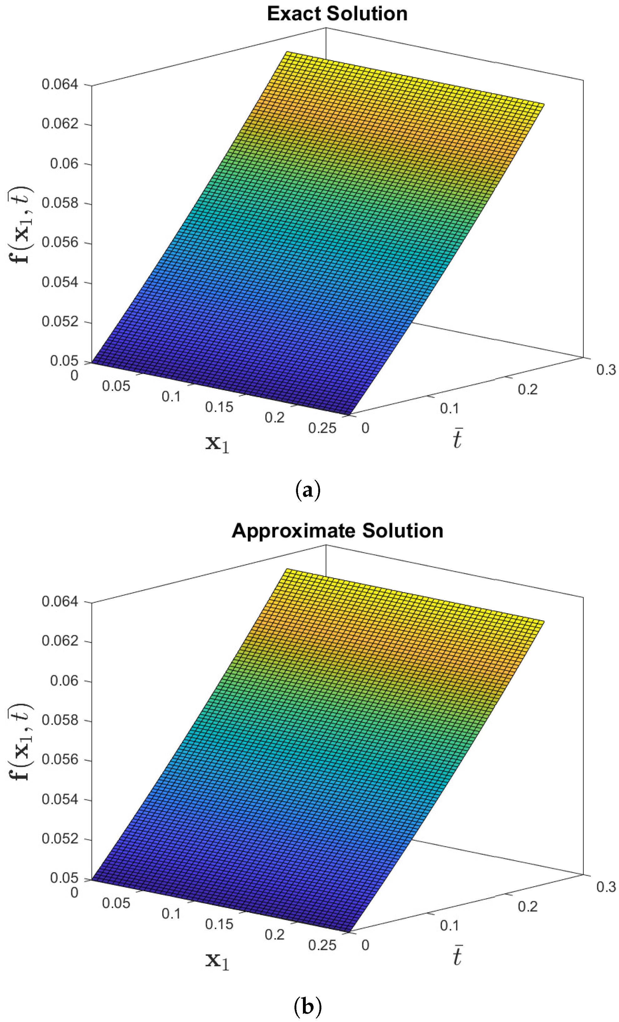
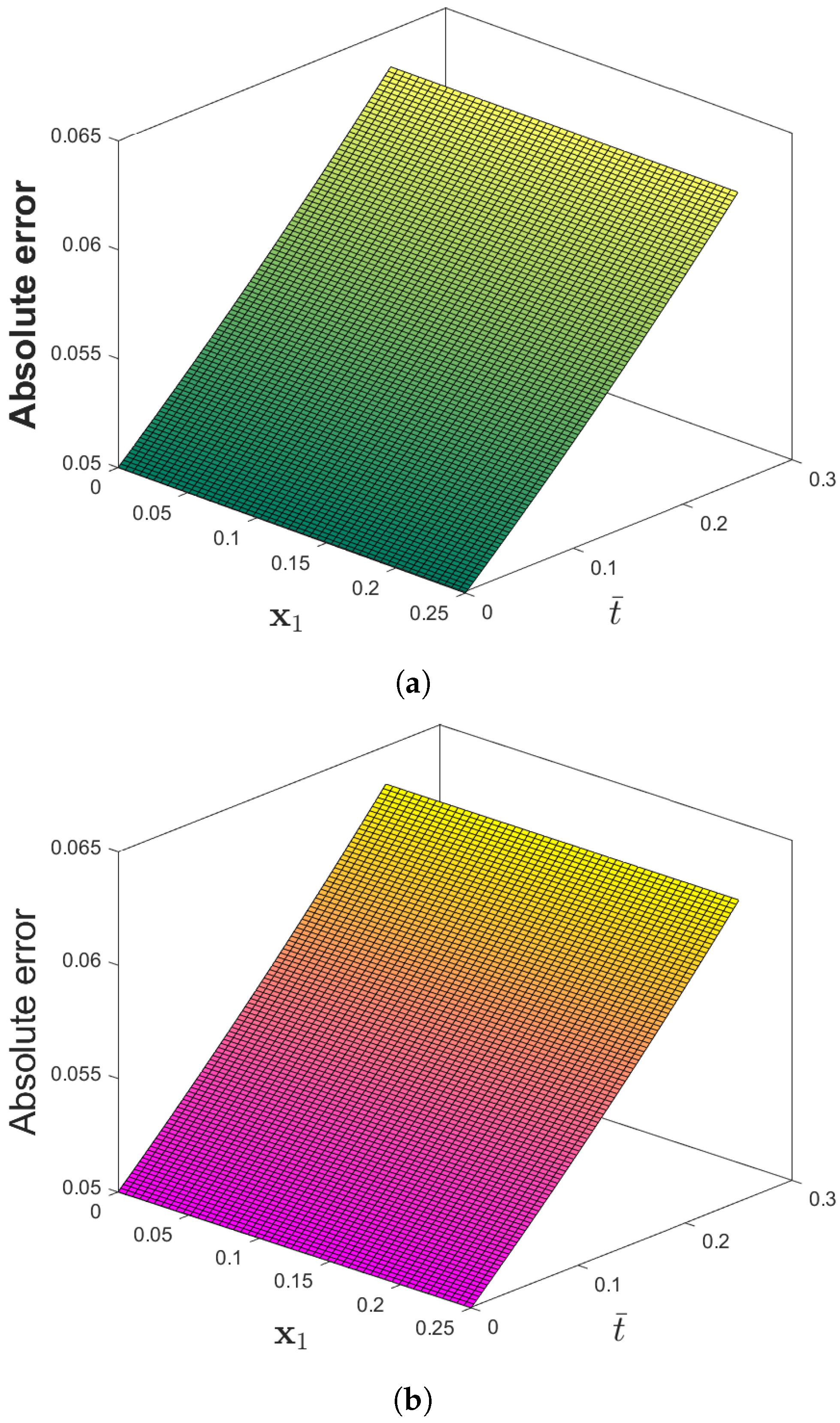
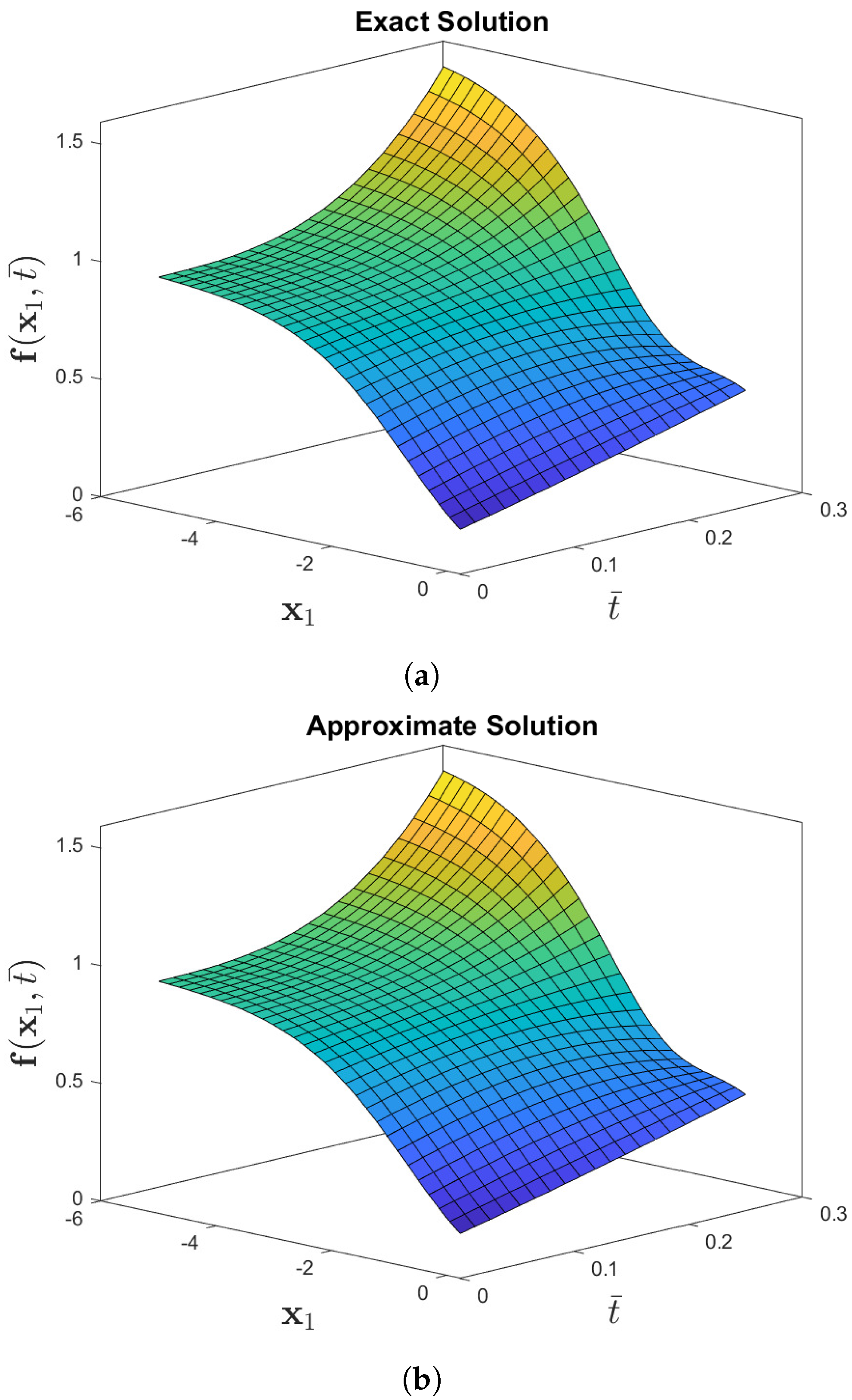
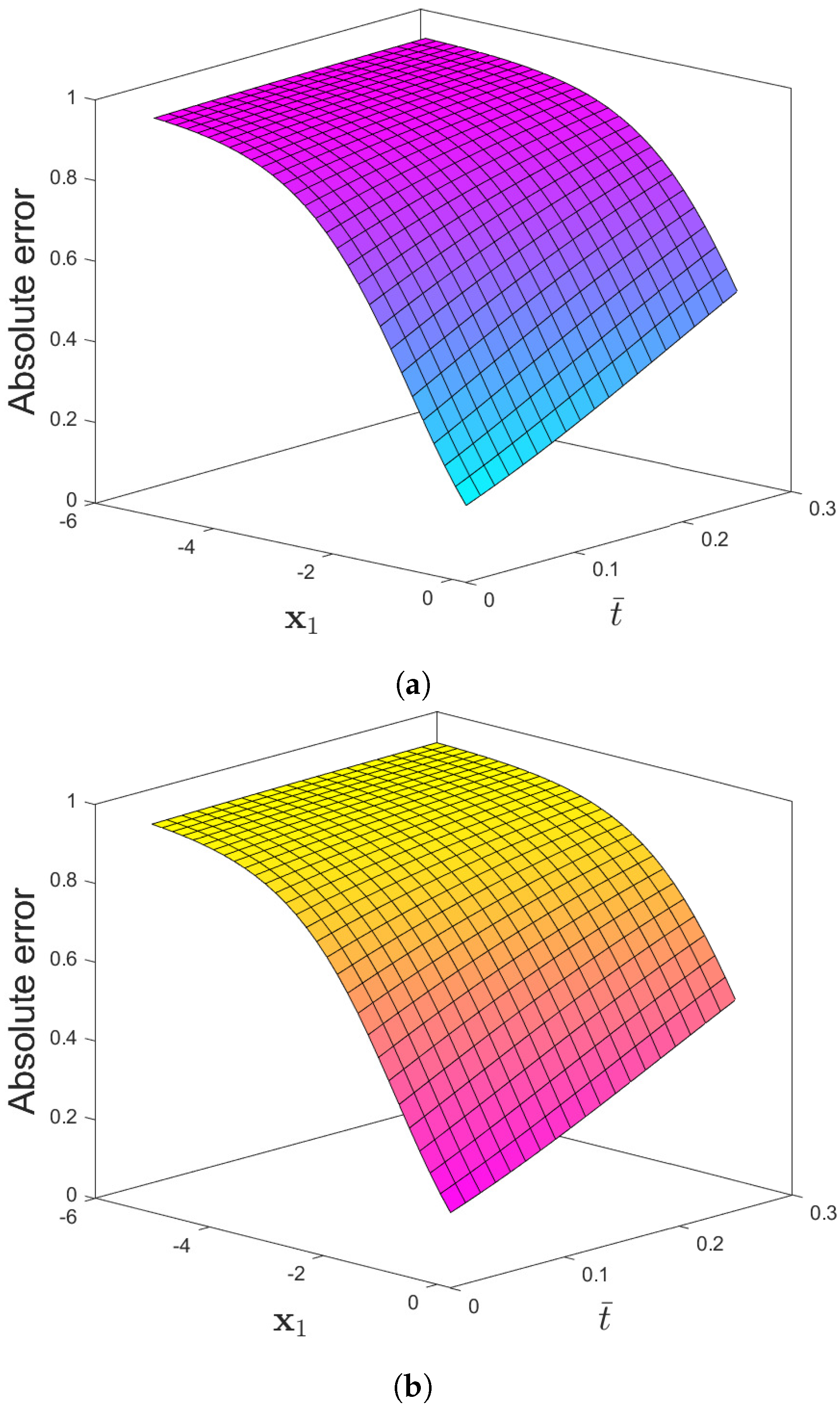
4. Evaluation of the Fractional Fisher Model via IETM

This section demonstrate the reliability and preciseness of the projected methodology.

Problem 1.

If $\theta =1,\beta =1$, and $\phi =0$ in (10) with ${\mathbf{f}}_0({\mathbf{x}}_1,0)=\eta ,$ then the one dimensional time fractional Fisher equation is presented as follows.

$$\begin{array}{c}\hfill \frac{{\partial }^{\alpha }\mathbf{f}}{\partial {\overline{t}}^{\alpha }}=\frac{{\partial }^2\mathbf{f}}{\partial {\mathbf{x}}_1^2}+\mathbf{f}(1-\mathbf{f}).\end{array}$$

(36)

The integer-order solution for the Fisher’s Equation (36) is obtained by using the Taylor’s series expansion for $\alpha =1$ as follows.

$$\mathbf{f}({\mathbf{x}}_1,\overline{t})=\frac{\eta exp\left(\overline{t}\right)}{1-\eta +\eta exp\left(\overline{t}\right)}.$$

Case I. First, we formulate Problem 1 by utilizing the Elzaki transform coupled with the Caputo derivative operator.

By employing the Elzaki transform to (36) with the initial condition, we have the following.

$$\begin{array}{c}\hfill \mathbb{E}\left[\frac{{\partial }^{\alpha }\mathbf{f}}{\partial {\overline{t}}^{\alpha }}\right]=\mathbb{E}\left[\frac{{\partial }^2\mathbf{f}}{\partial {\mathbf{x}}_1^2}+\mathbf{f}(1-\mathbf{f})\right].\end{array}$$

(37)

The following is the case:

$$\begin{array}{c}\hfill \frac{1}{{\omega }^{\alpha }}\mathbb{E}\left[\mathbf{f}({\mathbf{x}}_1,\overline{t})\right]-\sum _{\kappa =0}^{m-1}{\mathbf{f}}_{\left(\kappa \right)}({\mathbf{x}}_1,0){\omega }^{2-\alpha +\kappa }=\mathbb{E}\left[\frac{{\partial }^2\mathbf{f}}{\partial {\mathbf{x}}_1^2}+\mathbf{f}(1-\mathbf{f})\right].\end{array}$$

equivalently, we have

$$\begin{array}{c}\hfill \frac{1}{{\omega }^{\alpha }}\mathbb{E}\left[\mathbf{f}({\mathbf{x}}_1,\overline{t})\right]={\mathbf{f}}_{\left(0\right)}({\mathbf{x}}_1,0){\omega }^{2-\alpha }+\mathbb{E}\left[\frac{{\partial }^2\mathbf{f}}{\partial {\mathbf{x}}_1^2}+\mathbf{f}(1-\mathbf{f})\right].\end{array}$$

Using the inverse Elzaki transform, we have the following.

$$\begin{array}{c}\hfill \mathbf{f}({\mathbf{x}}_1,\overline{t})=\eta +{\mathbb{E}}^{-1}\left[{\omega }^{\alpha }\mathbb{E}\left[\frac{{\partial }^2\mathbf{f}}{\partial {\mathbf{x}}_1^2}+\mathbf{f}(1-\mathbf{f})\right]\right].\end{array}$$

Applying the iterative technique described in Section 3.1, we obtain the following.

$$\begin{array}{ccc}\hfill {\mathbf{f}}_0({\mathbf{x}}_1,\overline{t})& & =\eta ,\hfill \\ \hfill {\mathbf{f}}_1({\mathbf{x}}_1,\overline{t})& & ={\mathbb{E}}^{-1}\left[{\omega }^{\alpha }\mathbb{E}\left\{{\left({\mathbf{f}}_0({\mathbf{x}}_1,\overline{t})\right)}_{{\mathbf{x}}_1{\mathbf{x}}_1}+{\mathbf{f}}_0(1-{\mathbf{f}}_0)\right\}\right]\hfill \\ & & =\eta (1-\eta )\frac{{\overline{t}}^{\alpha }}{\Gamma (\alpha +1)},\hfill \\ \hfill {\mathbf{f}}_2({\mathbf{x}}_1,\overline{t})& & ={\mathbb{E}}^{-1}\left[{\omega }^{\alpha }\mathbb{E}\left\{{\left({\mathbf{f}}_1({\mathbf{x}}_1,\overline{t})\right)}_{{\mathbf{x}}_1{\mathbf{x}}_1}+{\mathbf{f}}_1(1-{\mathbf{f}}_1)\right\}\right]\hfill \\ & & =\eta (1-\eta )(1-2\eta )\frac{{\overline{t}}^{2\alpha }}{\Gamma (2\alpha +1)},\hfill \\ \hfill {\mathbf{f}}_3({\mathbf{x}}_1,\overline{t})& & ={\mathbb{E}}^{-1}\left[{\omega }^{\alpha }\mathbb{E}\left\{{\left({\mathbf{f}}_2({\mathbf{x}}_1,\overline{t})\right)}_{{\mathbf{x}}_1{\mathbf{x}}_1}+{\mathbf{f}}_2(1-{\mathbf{f}}_2)\right\}\right]\hfill \\ & & =\eta (1-\eta )(1-6\eta +6{\eta }^2)\frac{{\overline{t}}^{3\alpha }}{\Gamma (3\alpha +1)},\hfill \\ \hfill {\mathbf{f}}_4({\mathbf{x}}_1,\overline{t})& & ={\mathbb{E}}^{-1}\left[{\omega }^{\alpha }\mathbb{E}\left\{{\left({\mathbf{f}}_3({\mathbf{x}}_1,\overline{t})\right)}_{{\mathbf{x}}_1{\mathbf{x}}_1}+{\mathbf{f}}_3(1-{\mathbf{f}}_3)\right\}\right]\hfill \\ & & =\eta (1-\eta )(1-2\eta )(1-12\eta +12{\eta }^2)\frac{{\overline{t}}^{4\alpha }}{\Gamma (4\alpha +1)},\hfill \\ \hfill ⋮\end{array}$$

Provided that the series form solution is as follows:

$$\begin{array}{c}\hfill \mathbf{f}({\mathbf{x}}_1,\overline{t})={\mathbf{f}}_0({\mathbf{x}}_1,\overline{t})+{\mathbf{f}}_1({\mathbf{x}}_1,\overline{t})+{\mathbf{f}}_2({\mathbf{x}}_1,\overline{t})+{\mathbf{f}}_3({\mathbf{x}}_1,\overline{t})+\dots +{\mathbf{f}}_{m_1}({\mathbf{x}}_1,\overline{t}).\end{array}$$

we consequently have

$$\begin{array}{ccc}\hfill \mathbf{f}({\mathbf{x}}_1,\overline{t})& & =\eta +\eta (1-\eta )\frac{{\overline{t}}^{\alpha }}{\Gamma (\alpha +1)}+\eta (1-\eta )(1-2\eta )\frac{{\overline{t}}^{2\alpha }}{\Gamma (2\alpha +1)}+\eta (1-\eta )(1-6\eta +6{\eta }^2)\frac{{\overline{t}}^{3\alpha }}{\Gamma (3\alpha +1)}\hfill \\ & & +\eta (1-\eta )(1-2\eta )(1-12\eta +12{\eta }^2)\frac{{\overline{t}}^{4\alpha }}{\Gamma (4\alpha +1)}+\dots \hfill \end{array}$$

Case II. Now we formulate Problem 1 by utilizing Elzaki transform coupled with the ABC derivative operator.

By employing the Elzaki transform to (36) with the initial condition, we have the following.

$$\begin{array}{c}\hfill \mathbb{E}\left[\frac{{\partial }^{\alpha }\mathbf{f}}{\partial {\overline{t}}^{\alpha }}\right]=\mathbb{E}\left[\frac{{\partial }^2\mathbf{f}}{\partial {\mathbf{x}}_1^2}+\mathbf{f}(1-\mathbf{f})\right].\end{array}$$

(38)

The following is then the case.

$$\begin{array}{c}\hfill \mathbb{E}\left[\mathbf{f}({\mathbf{x}}_1,\overline{t})\right]={\mathbf{f}}_{\left(0\right)}({\mathbf{x}}_1,0){\omega }^2+\frac{\alpha {\omega }^{\alpha }+1-\alpha }{\mathbb{N}\left(\alpha \right)}\mathbb{E}\left[\frac{{\partial }^2\mathbf{f}}{\partial {\mathbf{x}}_1^2}+\mathbf{f}(1-\mathbf{f})\right].\end{array}$$

Using the inverse Elzaki transform, we have the following.

$$\begin{array}{c}\hfill \mathbf{f}({\mathbf{x}}_1,\overline{t})=\eta +{\mathbb{E}}^{-1}\left[\frac{\alpha {\omega }^{\alpha }+1-\alpha }{\mathbb{N}\left(\alpha \right)}\mathbb{E}\left[\frac{{\partial }^2\mathbf{f}}{\partial {\mathbf{x}}_1^2}+\mathbf{f}(1-\mathbf{f})\right]\right].\end{array}$$

Applying the iterative technique described in Section 3.1, we obtain the following results.

$$\begin{array}{ccc}\hfill {\mathbf{f}}_0({\mathbf{x}}_1,\overline{t})& & =\eta ,\hfill \\ \hfill {\mathbf{f}}_1({\mathbf{x}}_1,\overline{t})& & ={\mathbb{E}}^{-1}\left[\frac{\alpha {\omega }^{\alpha }+1-\alpha }{\mathbb{N}\left(\alpha \right)}\mathbb{E}\left\{{\left({\mathbf{f}}_0({\mathbf{x}}_1,\overline{t})\right)}_{{\mathbf{x}}_1{\mathbf{x}}_1}+{\mathbf{f}}_0(1-{\mathbf{f}}_0)\right\}\right]\hfill \\ & & =\frac{\eta (1-\eta )}{\mathbb{N}\left(\alpha \right)}\left[\frac{\alpha {\overline{t}}^{\alpha }}{\Gamma (\alpha +1)}+(1-\alpha )\right],\hfill \\ \hfill {\mathbf{f}}_2({\mathbf{x}}_1,\overline{t})& & ={\mathbb{E}}^{-1}\left[\frac{\alpha {\omega }^{\alpha }+1-\alpha }{\mathbb{N}\left(\alpha \right)}\mathbb{E}\left\{{\left({\mathbf{f}}_1({\mathbf{x}}_1,\overline{t})\right)}_{{\mathbf{x}}_1{\mathbf{x}}_1}+{\mathbf{f}}_1(1-{\mathbf{f}}_1)\right\}\right]\hfill \\ & & =\frac{\eta (1-\eta )(1-2\eta )}{{\mathbb{N}}^2\left(\alpha \right)}\left[\frac{{\alpha }^2{\overline{t}}^{2\alpha }}{\Gamma (2\alpha +1)}+2\alpha (1-\alpha )\frac{{\overline{t}}^{\alpha }}{\Gamma (\alpha +1)}+{(1-\alpha )}^2\right],\hfill \\ \hfill {\mathbf{f}}_3({\mathbf{x}}_1,\overline{t})& & ={\mathbb{E}}^{-1}\left[\frac{\alpha {\omega }^{\alpha }+1-\alpha }{\mathbb{N}\left(\alpha \right)}\mathbb{E}\left\{{\left({\mathbf{f}}_2({\mathbf{x}}_1,\overline{t})\right)}_{{\mathbf{x}}_1{\mathbf{x}}_1}+{\mathbf{f}}_2(1-{\mathbf{f}}_2)\right\}\right]\hfill \\ & & =\frac{\eta (1-\eta )(1-6\eta +6{\eta }^2)}{{\mathbb{N}}^3\left(\alpha \right)}\left[\frac{{\alpha }^3{\overline{t}}^{3\alpha }}{\Gamma (3\alpha +1)}+3{\alpha }^2(1-\alpha )\frac{{\overline{t}}^{2\alpha }}{\Gamma (2\alpha +1)}+3\alpha {(1-\alpha )}^2\frac{{\overline{t}}^{\alpha }}{\Gamma (\alpha +1)}+{(1-\alpha )}^3\right],\hfill \\ \hfill ⋮\end{array}$$

Provided the series form solution is as follows:

$$\begin{array}{c}\hfill \mathbf{f}({\mathbf{x}}_1,\overline{t})={\mathbf{f}}_0({\mathbf{x}}_1,\overline{t})+{\mathbf{f}}_1({\mathbf{x}}_1,\overline{t})+{\mathbf{f}}_2({\mathbf{x}}_1,\overline{t})+{\mathbf{f}}_3({\mathbf{x}}_1,\overline{t})+\dots +{\mathbf{f}}_{m_1}({\mathbf{x}}_1,\overline{t}).\end{array}$$

we consequently have

$$\begin{array}{ccc}\hfill \mathbf{f}({\mathbf{x}}_1,\overline{t})& & =\eta +\frac{\eta (1-\eta )}{\mathbb{N}\left(\alpha \right)}\left[\frac{\alpha {\overline{t}}^{\alpha }}{\Gamma (\alpha +1)}+(1-\alpha )\right]+\frac{\eta (1-\eta )(1-2\eta )}{{\mathbb{N}}^2\left(\alpha \right)}\left[\frac{{\alpha }^2{\overline{t}}^{2\alpha }}{\Gamma (2\alpha +1)}+2\alpha (1-\alpha )\frac{{\overline{t}}^{\alpha }}{\Gamma (\alpha +1)}+{(1-\alpha )}^2\right]\hfill \\ & & +\frac{\eta (1-\eta )(1-6\eta +6{\eta }^2)}{{\mathbb{N}}^3\left(\alpha \right)}\left[\frac{{\alpha }^3{\overline{t}}^{3\alpha }}{\Gamma (3\alpha +1)}+3{\alpha }^2(1-\alpha )\frac{{\overline{t}}^{2\alpha }}{\Gamma (2\alpha +1)}+3\alpha {(1-\alpha )}^2\frac{{\overline{t}}^{\alpha }}{\Gamma (\alpha +1)}+{(1-\alpha )}^3\right]+\dots \hfill \end{array}$$

For showing the accuracy and compactness of our proposed algorithm (IETM via CFD and ABC fractional derivatives), we compare our results with [39]. It can be observed from

Table 1. Comparison results with exact $\left({\mathbf{f}}_E\right)$ IETM-numerical solutions $\left({\mathbf{f}}_{Num}\right)$ for CFD and ABC fractional derivative operator of $\mathbf{f}({\mathbf{x}}_1,\overline{t})$ of Case 1 with absolute errors and the HPM [39] when $\alpha =1,$$\overline{t}=0.01,$$\eta =0.05$, and $\phi =0$ for various values of ${\mathbf{x}}_1.$

$\mathit{\eta }$	${\mathbf{f}}_{\mathit{E}}$	${\mathbf{f}}_{\mathit{Num}/\mathit{CFD}}$ sol.	${\mathbf{f}}_{\mathit{Num}/\mathit{ABC}}$ sol.	$|{\mathbf{f}}_{\mathit{E}}-{\mathbf{f}}_{\mathit{Num}/\mathit{CFD}}|$	$|{\mathbf{f}}_{\mathit{E}}-{\mathbf{f}}_{\mathit{Num}/\mathit{ABC}}|$	HPM sol. [39]
0.1	1.009 $\times {10}^{-1}$	1.009 $\times {10}^{-1}$	2.329 $\times {10}^{-1}$	0	1.319 $\times {10}^{-1}$	8.999 × ${10}^{-1}$
0.2	2.016 $\times {10}^{-1}$	2.016 $\times {10}^{-1}$	4.091 $\times {10}^{-1}$	0	2.017 $\times {10}^{-1}$	7.987 $\times {10}^{-1}$
0.3	3.021 $\times {10}^{-1}$	3.021 $\times {10}^{-1}$	5.429 $\times {10}^{-1}$	0	2.408 $\times {10}^{-1}$	9.210 $\times {10}^{-1}$
0.4	4.024 $\times {10}^{-1}$	4.024 $\times {10}^{-1}$	6.464 $\times {10}^{-1}$	1.00 $\times {10}^{-11}$	2.440 $\times {10}^{-1}$	7.540 $\times {10}^{-1}$
0.5	5.025 $\times {10}^{-1}$	5.025 $\times {10}^{-1}$	7.292 $\times {10}^{-1}$	3.00 $\times {10}^{-10}$	2.267 $\times {10}^{-1}$	8.908 $\times {10}^{-1}$
0.6	6.024 $\times {10}^{-1}$	6.024 $\times {10}^{-1}$	7.984 $\times {10}^{-1}$	1.00 $\times {10}^{-10}$	1.960 $\times {10}^{-1}$	9.765 $\times {10}^{-1}$
0.7	7.021 $\times {10}^{-1}$	7.021 $\times {10}^{-1}$	8.589 $\times {10}^{-1}$	0	1.568 $\times {10}^{-1}$	9.344 $\times {10}^{-1}$
0.8	8.016 $\times {10}^{-1}$	8.016 $\times {10}^{-1}$	9.131 $\times {10}^{-1}$	3.00 $\times {10}^{-10}$	1.115 $\times {10}^{-1}$	9.123 $\times {10}^{-1}$
0.9	9.009 $\times {10}^{-1}$	9.009 $\times {10}^{-1}$	9.609 $\times {10}^{-1}$	3.00 $\times {10}^{-10}$	6.000 $\times {10}^{-2}$	9.777 $\times {10}^{-1}$
1.0	1.000 $\times {10}^0$	1.000 $\times {10}^0$	1.000 $\times {10}^0$	0	0	1.000 $\times {10}^0$

that the present algorithm is very effective and yields accurate results. The absolute errors of the numerical solution of Fisher’s equation obtained by IETM (CFD and ABC fractional derivatives) and the exact solutions for Case 1 are depicted in Table 1 and presents a strong correlation among the proposed technique and rapidly converges to the exact solution very efficiently in a short admissible domain.

Figure 1 compares the exact and approximate solutions to Problem 1 using the CDF operator. The absolute error norm in Figure 2 for (36) with the assumptions of $\eta$ = 0.05, $\theta$ = 1, $\beta =1$, and $\phi =0$ ensures the approximation of the numerical results derived by IETM to the exact solution via the CFD and ABC fractional derivative operators, respectively. The results of the graphical representation reveal that the model is highly dependent on fractional order $\alpha$. The absolute inaccuracy is really small. Two dimensional representations of graphs via Figure 3 show the strong connection between the exact and approximate solutions for various fractional orders. Furthermore, Figure 3a,b illustrate that the ABC fractional derivative operator has better harmony than the CFD operator.

Problem 2.

If $\theta =6,\beta =1$ and $\phi =0$ in (10) with ${\mathbf{f}}_0({\mathbf{x}}_1,0)=\frac{1}{{(1+exp\left({\mathbf{x}}_1\right))}^2},$ then the one dimensional time fractional Fisher equation is presented as follows.

$$\begin{array}{c}\hfill \frac{{\partial }^{\alpha }\mathbf{f}}{\partial {\overline{t}}^{\alpha }}=\frac{{\partial }^2\mathbf{f}}{\partial {\mathbf{x}}_1^2}+6\mathbf{f}(1-\mathbf{f}).\end{array}$$

(39)

The integer-order solution for the Fisher’s Equation (39) is obtained by using the Taylor’s series expansion for $\alpha =1$ as follows.

$$\mathbf{f}({\mathbf{x}}_1,\overline{t})=\frac{1}{{(1+exp({\mathbf{x}}_1-5\overline{t}))}^2}.$$

Case I. First, we formulate Problem 2 by utilizing the Elzaki transform coupled with the Caputo derivative operator.

Employing the Elzaki transform to (39) with the initial condition, we have the following.

$$\begin{array}{c}\hfill \mathbb{E}\left[\frac{{\partial }^{\alpha }\mathbf{f}}{\partial {\overline{t}}^{\alpha }}\right]=\mathbb{E}\left[\frac{{\partial }^2\mathbf{f}}{\partial {\mathbf{x}}_1^2}+6\mathbf{f}(1-\mathbf{f})\right].\end{array}$$

(40)

The following results:

$$\begin{array}{c}\hfill \frac{1}{{\omega }^{\alpha }}\mathbb{E}\left[\mathbf{f}({\mathbf{x}}_1,\overline{t})\right]-\sum _{\kappa =0}^{m-1}{\mathbf{f}}_{\left(\kappa \right)}({\mathbf{x}}_1,0){\omega }^{2-\alpha +\kappa }=\mathbb{E}\left[\frac{{\partial }^2\mathbf{f}}{\partial {\mathbf{x}}_1^2}+6\mathbf{f}(1-\mathbf{f})\right].\end{array}$$

equivalently, we have

$$\begin{array}{c}\hfill \frac{1}{{\omega }^{\alpha }}\mathbb{E}\left[\mathbf{f}({\mathbf{x}}_1,\overline{t})\right]={\mathbf{f}}_{\left(0\right)}({\mathbf{x}}_1,0){\omega }^{2-\alpha }+\mathbb{E}\left[\frac{{\partial }^2\mathbf{f}}{\partial {\mathbf{x}}_1^2}+6\mathbf{f}(1-\mathbf{f})\right].\end{array}$$

Using the inverse Elzaki transform, we have the following.

$$\begin{array}{c}\hfill \mathbf{f}({\mathbf{x}}_1,\overline{t})=\eta +{\mathbb{E}}^{-1}\left[{\omega }^{\alpha }\mathbb{E}\left[\frac{{\partial }^2\mathbf{f}}{\partial {\mathbf{x}}_1^2}+6\mathbf{f}(1-\mathbf{f})\right]\right].\end{array}$$

Applying the iterative technique described in Section 3.1, we obtain the following.

$$\begin{array}{ccc}\hfill {\mathbf{f}}_0({\mathbf{x}}_1,\overline{t})& & =\frac{1}{{(1+exp\left({\mathbf{x}}_1\right))}^2},\hfill \\ \hfill {\mathbf{f}}_1({\mathbf{x}}_1,\overline{t})& & ={\mathbb{E}}^{-1}\left[{\omega }^{\alpha }\mathbb{E}\left\{{\left({\mathbf{f}}_0({\mathbf{x}}_1,\overline{t})\right)}_{{\mathbf{x}}_1{\mathbf{x}}_1}+6{\mathbf{f}}_0(1-{\mathbf{f}}_0)\right\}\right]\hfill \\ & & =\frac{10exp\left({\mathbf{x}}_1\right)}{{(1+exp\left({\mathbf{x}}_1\right))}^3}\frac{{\overline{t}}^{\alpha }}{\Gamma (\alpha +1)},\hfill \\ \hfill {\mathbf{f}}_2({\mathbf{x}}_1,\overline{t})& & ={\mathbb{E}}^{-1}\left[{\omega }^{\alpha }\mathbb{E}\left\{{\left({\mathbf{f}}_1({\mathbf{x}}_1,\overline{t})\right)}_{{\mathbf{x}}_1{\mathbf{x}}_1}+6{\mathbf{f}}_1(1-{\mathbf{f}}_1)\right\}\right]\hfill \\ & & =\frac{50exp\left({\mathbf{x}}_1\right)(exp\left(2{\mathbf{x}}_1\right)-1)}{{(1+exp\left({\mathbf{x}}_1\right))}^4}\frac{{\overline{t}}^{2\alpha }}{\Gamma (2\alpha +1)},\hfill \\ \hfill {\mathbf{f}}_3({\mathbf{x}}_1,\overline{t})& & ={\mathbb{E}}^{-1}\left[{\omega }^{\alpha }\mathbb{E}\left\{{\left({\mathbf{f}}_2({\mathbf{x}}_1,\overline{t})\right)}_{{\mathbf{x}}_1{\mathbf{x}}_1}+6{\mathbf{f}}_2(1-{\mathbf{f}}_2)\right\}\right]\hfill \\ & & =-\frac{750(7exp\left({\mathbf{x}}_1\right)-4exp\left(2{\mathbf{x}}_1\right)-1)}{3{(1+exp\left({\mathbf{x}}_1\right))}^5}\frac{{\overline{t}}^{3\alpha }}{\Gamma (3\alpha +1)},\hfill \\ \hfill ⋮\end{array}$$

Provided the series form solution is the following:

$$\begin{array}{c}\hfill \mathbf{f}({\mathbf{x}}_1,\overline{t})={\mathbf{f}}_0({\mathbf{x}}_1,\overline{t})+{\mathbf{f}}_1({\mathbf{x}}_1,\overline{t})+{\mathbf{f}}_2({\mathbf{x}}_1,\overline{t})+{\mathbf{f}}_3({\mathbf{x}}_1,\overline{t})+\dots +{\mathbf{f}}_{m_1}({\mathbf{x}}_1,\overline{t}).\end{array}$$

we consequently have the following.

$$\begin{array}{ccc}\hfill \mathbf{f}({\mathbf{x}}_1,\overline{t})& & =\frac{1}{{(1+exp\left({\mathbf{x}}_1\right))}^2}+\frac{10exp\left({\mathbf{x}}_1\right)}{{(1+exp\left({\mathbf{x}}_1\right))}^3}\frac{{\overline{t}}^{\alpha }}{\Gamma (\alpha +1)}+\frac{50exp\left({\mathbf{x}}_1\right)(exp\left(2{\mathbf{x}}_1\right)-1)}{{(1+exp\left({\mathbf{x}}_1\right))}^4}\frac{{\overline{t}}^{2\alpha }}{\Gamma (2\alpha +1)}\hfill \\ & & -\frac{570(7exp\left({\mathbf{x}}_1\right)-4exp\left(2{\mathbf{x}}_1\right)-1)}{3{(1+exp\left({\mathbf{x}}_1\right))}^5}\frac{{\overline{t}}^{3\alpha }}{\Gamma (3\alpha +1)}+\dots \hfill \end{array}$$

Case II. Now we formulate Problem 2 by utilizing the Elzaki transform coupled with an ABC derivative operator.

Employing the Elzaki transform to (39) with the initial condition, we have the following.

$$\begin{array}{c}\hfill \mathbb{E}\left[\frac{{\partial }^{\alpha }\mathbf{f}}{\partial {\overline{t}}^{\alpha }}\right]=\mathbb{E}\left[\frac{{\partial }^2\mathbf{f}}{\partial {\mathbf{x}}_1^2}+6\mathbf{f}(1-\mathbf{f})\right].\end{array}$$

(41)

$$\begin{array}{c}\hfill \mathbb{E}\left[\mathbf{f}({\mathbf{x}}_1,\overline{t})\right]={\mathbf{f}}_{\left(0\right)}({\mathbf{x}}_1,0){\omega }^2+\frac{\alpha {\omega }^{\alpha }+(1-\alpha )}{\mathbb{N}\left(\alpha \right)}\mathbb{E}\left[\frac{{\partial }^2\mathbf{f}}{\partial {\mathbf{x}}_1^2}+6\mathbf{f}(1-\mathbf{f})\right].\end{array}$$

By using the inverse Elzaki transform, we have the following.

$$\begin{array}{c}\hfill \mathbf{f}({\mathbf{x}}_1,\overline{t})=\eta +{\mathbb{E}}^{-1}\left[\frac{\alpha {\omega }^{\alpha }+(1-\alpha )}{\mathbb{N}\left(\alpha \right)}\mathbb{E}\left[\frac{{\partial }^2\mathbf{f}}{\partial {\mathbf{x}}_1^2}+6\mathbf{f}(1-\mathbf{f})\right]\right].\end{array}$$

By applying the iterative technique described in Section 3.1, we obtain the following.

$$\begin{array}{ccc}\hfill {\mathbf{f}}_0({\mathbf{x}}_1,\overline{t})& & =\frac{1}{{(1+exp\left({\mathbf{x}}_1\right))}^2},\hfill \\ \hfill {\mathbf{f}}_1({\mathbf{x}}_1,\overline{t})& & ={\mathbb{E}}^{-1}\left[\frac{\alpha {\omega }^{\alpha }+(1-\alpha )}{\mathbb{N}\left(\alpha \right)}\mathbb{E}\left\{{\left({\mathbf{f}}_0({\mathbf{x}}_1,\overline{t})\right)}_{{\mathbf{x}}_1{\mathbf{x}}_1}+6{\mathbf{f}}_0(1-{\mathbf{f}}_0)\right\}\right]\hfill \\ & & =\frac{10exp\left({\mathbf{x}}_1\right)}{\mathbb{N}\left(\alpha \right){(1+exp\left({\mathbf{x}}_1\right))}^3}\left[\frac{\alpha {\overline{t}}^{\alpha }}{\Gamma (\alpha +1)}+(1-\alpha )\right],\hfill \\ \hfill {\mathbf{f}}_2({\mathbf{x}}_1,\overline{t})& & ={\mathbb{E}}^{-1}\left[\frac{\alpha {\omega }^{\alpha }+(1-\alpha )}{\mathbb{N}\left(\alpha \right)}\mathbb{E}\left\{{\left({\mathbf{f}}_1({\mathbf{x}}_1,\overline{t})\right)}_{{\mathbf{x}}_1{\mathbf{x}}_1}+6{\mathbf{f}}_1(1-{\mathbf{f}}_1)\right\}\right]\hfill \\ & & =\frac{50exp\left({\mathbf{x}}_1\right)(exp\left(2{\mathbf{x}}_1\right)-1)}{{\mathbb{N}}^2\left(\alpha \right){(1+exp\left({\mathbf{x}}_1\right))}^4}\left[\frac{{\alpha }^2{\overline{t}}^{2\alpha }}{\Gamma (2\alpha +1)}+2\alpha (1-\alpha )\frac{{\overline{t}}^{\alpha }}{\Gamma (1+\alpha )}+{(1-\alpha )}^2\right],\hfill \\ \hfill {\mathbf{f}}_3({\mathbf{x}}_1,\overline{t})& & ={\mathbb{E}}^{-1}\left[\frac{\alpha {\omega }^{\alpha }+(1-\alpha )}{\mathbb{N}\left(\alpha \right)}\mathbb{E}\left\{{\left({\mathbf{f}}_2({\mathbf{x}}_1,\overline{t})\right)}_{{\mathbf{x}}_1{\mathbf{x}}_1}+6{\mathbf{f}}_2(1-{\mathbf{f}}_2)\right\}\right]\hfill \\ & & =-\frac{750(7exp\left({\mathbf{x}}_1\right)-4exp\left(2{\mathbf{x}}_1\right)-1)}{3{\mathbb{N}}^3\left(\alpha \right){(1+exp\left({\mathbf{x}}_1\right))}^5}\hfill \\ & & \times \left[\frac{{\alpha }^3{\overline{t}}^{3\alpha }}{\Gamma (3\alpha +1)}+3{\alpha }^2(1-\alpha )\frac{{\overline{t}}^{2\alpha }}{\Gamma (1+2\alpha )}+3\alpha {(1-\alpha )}^2\frac{{\overline{t}}^{\alpha }}{\Gamma (1+\alpha )}+{(1-\alpha )}^3\right],\hfill \\ \hfill ⋮\end{array}$$

Provided that the series form solution is as follows:

$$\begin{array}{c}\hfill \mathbf{f}({\mathbf{x}}_1,\overline{t})={\mathbf{f}}_0({\mathbf{x}}_1,\overline{t})+{\mathbf{f}}_1({\mathbf{x}}_1,\overline{t})+{\mathbf{f}}_2({\mathbf{x}}_1,\overline{t})+{\mathbf{f}}_3({\mathbf{x}}_1,\overline{t})+\dots +{\mathbf{f}}_{m_1}({\mathbf{x}}_1,\overline{t}).\end{array}$$

the following consequently results.

$$\begin{array}{ccc}\hfill \mathbf{f}({\mathbf{x}}_1,\overline{t})& & =\frac{1}{{(1+exp\left({\mathbf{x}}_1\right))}^2}+\frac{10exp\left({\mathbf{x}}_1\right)}{\mathbb{N}\left(\alpha \right){(1+exp\left({\mathbf{x}}_1\right))}^3}\left[\frac{\alpha {\overline{t}}^{\alpha }}{\Gamma (\alpha +1)}+(1-\alpha )\right]\hfill \\ & & +\frac{50exp\left({\mathbf{x}}_1\right)(exp\left(2{\mathbf{x}}_1\right)-1)}{{\mathbb{N}}^2\left(\alpha \right){(1+exp\left({\mathbf{x}}_1\right))}^4}\left[\frac{{\alpha }^2{\overline{t}}^{2\alpha }}{\Gamma (2\alpha +1)}+2\alpha (1-\alpha )\frac{{\overline{t}}^{\alpha }}{\Gamma (1+\alpha )}+{(1-\alpha )}^2\right]\hfill \\ & & -\frac{750(7exp\left({\mathbf{x}}_1\right)-4exp\left(2{\mathbf{x}}_1\right)-1)}{3{\mathbb{N}}^3\left(\alpha \right){(1+exp\left({\mathbf{x}}_1\right))}^5}\hfill \\ & & \times \left[\frac{{\alpha }^3{\overline{t}}^{3\alpha }}{\Gamma (3\alpha +1)}+3{\alpha }^2(1-\alpha )\frac{{\overline{t}}^{2\alpha }}{\Gamma (1+2\alpha )}+3\alpha {(1-\alpha )}^2\frac{{\overline{t}}^{\alpha }}{\Gamma (1+\alpha )}+{(1-\alpha )}^3\right]+\dots \hfill \end{array}$$

For showing the accuracy and compactness of our proposed algorithm (IETM via CFD and ABC fractional derivatives), we compare our results with [39]. It can be observed from

Table 2. Comparison results with exact $\left({\mathbf{f}}_E\right)$ IETM-numerical solutions $\left({\mathbf{f}}_{Num}\right)$ for CFD and ABC fractional derivative operator of $\mathbf{f}({\mathbf{x}}_1,\overline{t})$ of Case 2 with absolute errors and the HPM [39] when $\alpha =1,$$\overline{t}=0.01$, and $\phi =0$ for various values of ${\mathbf{x}}_1.$

${\mathbf{x}}_1$	${\mathbf{f}}_{\mathit{E}}$	${\mathbf{f}}_{\mathit{Num}/\mathit{CFD}}$ sol.	${\mathbf{f}}_{\mathit{Num}/\mathit{ABC}}$ sol.	$|{\mathbf{f}}_{\mathit{E}}-{\mathbf{f}}_{\mathit{Num}/\mathit{CFD}}|$	$|{\mathbf{f}}_{\mathit{E}}-{\mathbf{f}}_{\mathit{Num}/\mathit{ABC}}|$	HPM sol. [39]
0.1	2.377 $\times {10}^{-1}$	2.375 $\times {10}^{-1}$	2.432 $\times {10}^{-1}$	1.394 $\times {10}^{-4}$	−5.7000 $\times {10}^{-4}$	8.387 $\times {10}^{-1}$
0.2	2.140 $\times {10}^{-1}$	2.138 $\times {10}^{-1}$	2.159 $\times {10}^{-1}$	1.119 $\times {10}^{-4}$	−0.019 $\times {10}^{-4}$	9.567 $\times {10}^{-1}$
0.3	1.917 $\times {10}^{-1}$	1.915 $\times {10}^{-1}$	2.000 $\times {10}^{-1}$	9.68 $\times {10}^{-5}$	−0.083 $\times {10}^{-5}$	4.534 $\times {10}^{-1}$
0.4	1.709 $\times {10}^{-1}$	1.708 $\times {10}^{-1}$	1.888 $\times {10}^{-1}$	7.32 $\times {10}^{-5}$	−0.179 $\times {10}^{-5}$	8.887 $\times {10}^{-1}$
0.5	1.516 $\times {10}^{-1}$	−0.18 $\times {10}^{-5}$	1.575 $\times {10}^{-1}$	4.85 $\times {10}^{-5}$	−0.059 $\times {10}^{-5}$	7.337 $\times {10}^{-1}$
0.6	1.339 $\times {10}^{-1}$	1.338 $\times {10}^{-1}$	1.958 $\times {10}^{-1}$	2.35 $\times {10}^{-5}$	−0.619 $\times {10}^{-5}$	9.337 $\times {10}^{-1}$
0.7	1.176 $\times {10}^{-1}$	1.175 $\times {10}^{-1}$	1.234 $\times {10}^{-1}$	4.85 $\times {10}^{-5}$	−0.58 $\times {10}^{-5}$	7.337 $\times {10}^{-1}$
0.8	1.029 $\times {10}^{-1}$	1.029 $\times {10}^{-1}$	1.416 $\times {10}^{-1}$	2.51 $\times {10}^{-5}$	−0.055 $\times {10}^{-5}$	9.998 $\times {10}^{-1}$
0.9	8.966 $\times {10}^{-2}$	8.971 $\times {10}^{-2}$	9.516 $\times {10}^{-1}$	4.76 $\times {10}^{-5}$	3.426 $\times {10}^{-5}$	9.001 $\times {10}^{-1}$
1.0	7.778 $\times {10}^{-1}$	7.784 $\times {10}^{-1}$	9.001 $\times {10}^0$	6.75 $\times {10}^{-5}$	−1.223 $\times {10}^{-5}$	7.337 $\times {10}^{-1}$

that the present algorithm is very effective and yields accurate results. The absolute errors of the numerical solution of Fisher’s equation obtained by IETM (CFD and ABC fractional derivatives) and the exact solutions for Case 2 are depicted in Table 2 and presents a strong correlation among the proposed technique and rapidly converges to the exact solution very efficiently in a short admissible domain.

Figure 4 compares the exact and approximate solutions to Problem 2 by using the CDF operator. The absolute error norm in Figure 5 for (39) with the assumptions of $\theta =6,\beta =1$, and $\phi =0$ ensures the approximation of the numerical results derived by the IETM to the exact solution via the CFD and ABC fractional derivative operators, respectively. The results of the graphical representation reveal that the model is highly dependent on fractional order $\alpha$. The absolute inaccuracy is really small. Surface and two dimensional representations of graphs via Figure 6 show the strong connection between the exact and approximate solutions for various fractional orders. Furthermore, Figure 6a,b illustrates that the ABC fractional derivative operator has better harmony than the CFD operator.

Problem 3.

If $\theta =1,\beta =6$, and $\phi =0$ in (10) with ${\mathbf{f}}_0({\mathbf{x}}_1,0)=\frac{1}{{(1+exp\left(\frac{3{\mathbf{x}}_1}{2}\right))}^{1/3}},$ then the one dimensional time fractional generalized Fisher’s equation is presented as follows.

$$\begin{array}{c}\hfill \frac{{\partial }^{\alpha }\mathbf{f}}{\partial {\overline{t}}^{\alpha }}=\frac{{\partial }^2\mathbf{f}}{\partial {\mathbf{x}}_1^2}+\mathbf{f}(1-{\mathbf{f}}^6).\end{array}$$

(42)

The integer-order solution for the Fisher’s Equation (42) is obtained by using the Taylor’s series expansion for $\alpha =1$ as follows.

$$\mathbf{f}({\mathbf{x}}_1,\overline{t})={\left(\frac{1}{2}\right)}^{1/3}{\left(tanh\left(\frac{15}{8}\overline{t}-\frac{3}{4}{\mathbf{x}}_1\right)+1\right)}^{1/3}.$$

Case I. First, we formulate Problem 3 by utilizing the Elzaki transform coupled with the Caputo derivative operator.

Employing the Elzaki transform to (42) with the initial condition, we have the following.

$$\begin{array}{c}\hfill \mathbb{E}\left[\frac{{\partial }^{\alpha }\mathbf{f}}{\partial {\overline{t}}^{\alpha }}\right]=\mathbb{E}\left[\frac{{\partial }^2\mathbf{f}}{\partial {\mathbf{x}}_1^2}+\mathbf{f}(1-{\mathbf{f}}^6)\right].\end{array}$$

(43)

The following is the case.

$$\begin{array}{c}\hfill \frac{1}{{\omega }^{\alpha }}\mathbb{E}\left[\mathbf{f}({\mathbf{x}}_1,\overline{t})\right]-\sum _{\kappa =0}^{m-1}{\mathbf{f}}_{\left(\kappa \right)}({\mathbf{x}}_1,0){\omega }^{2-\alpha +\kappa }=\mathbb{E}\left[\frac{{\partial }^2\mathbf{f}}{\partial {\mathbf{x}}_1^2}+\mathbf{f}(1-{\mathbf{f}}^6)\right].\end{array}$$

Equivalently, we have the following.

$$\begin{array}{c}\hfill \frac{1}{{\omega }^{\alpha }}\mathbb{E}\left[\mathbf{f}({\mathbf{x}}_1,\overline{t})\right]={\mathbf{f}}_{\left(0\right)}({\mathbf{x}}_1,0){\omega }^{2-\alpha }+\mathbb{E}\left[\frac{{\partial }^2\mathbf{f}}{\partial {\mathbf{x}}_1^2}+\mathbf{f}(1-{\mathbf{f}}^6)\right].\end{array}$$

By using the inverse Elzaki transform, we have the following.

$$\begin{array}{c}\hfill \mathbf{f}({\mathbf{x}}_1,\overline{t})=\frac{1}{{(1+exp\left(\frac{3{\mathbf{x}}_1}{2}\right))}^{1/3}}+{\mathbb{E}}^{-1}\left[{\omega }^{\alpha }\mathbb{E}\left[\frac{{\partial }^2\mathbf{f}}{\partial {\mathbf{x}}_1^2}+\mathbf{f}(1-{\mathbf{f}}^6)\right]\right].\end{array}$$

By applying the iterative technique described in Section 3.1, we obtain the following.

$$\begin{array}{ccc}\hfill {\mathbf{f}}_0({\mathbf{x}}_1,\overline{t})& & =\frac{1}{{(1+exp\left(\frac{3{\mathbf{x}}_1}{2}\right))}^{1/3}},\hfill \\ \hfill {\mathbf{f}}_1({\mathbf{x}}_1,\overline{t})& & ={\mathbb{E}}^{-1}\left[{\omega }^{\alpha }\mathbb{E}\left\{{\left({\mathbf{f}}_0({\mathbf{x}}_1,\overline{t})\right)}_{{\mathbf{x}}_1{\mathbf{x}}_1}+{\mathbf{f}}_0(1-{\mathbf{f}}_0^6)\right\}\right]\hfill \\ & & =\frac{5exp\left(\frac{3{\mathbf{x}}_1}{2}\right)}{4{(1+exp\left(\frac{3{\mathbf{x}}_1}{2}\right))}^{4/3}}\frac{{\overline{t}}^{\alpha }}{\Gamma (\alpha +1)},\hfill \\ \hfill {\mathbf{f}}_2({\mathbf{x}}_1,\overline{t})& & ={\mathbb{E}}^{-1}\left[{\omega }^{\alpha }\mathbb{E}\left\{{\left({\mathbf{f}}_1({\mathbf{x}}_1,\overline{t})\right)}_{{\mathbf{x}}_1{\mathbf{x}}_1}+{\mathbf{f}}_1(1-{\mathbf{f}}_1^6)\right\}\right]\hfill \\ & & =\frac{50exp\left(\frac{3{\mathbf{x}}_1}{2}\right)\left(exp\left(\frac{3x}{2}\right)-3\right)}{16{(1+exp\left(\frac{3{\mathbf{x}}_1}{2}\right))}^{7/3}}\frac{{\overline{t}}^{2\alpha }}{\Gamma (2\alpha +1)},\hfill \\ \hfill {\mathbf{f}}_3({\mathbf{x}}_1,\overline{t})& & ={\mathbb{E}}^{-1}\left[{\omega }^{\alpha }\mathbb{E}\left\{{\left({\mathbf{f}}_2({\mathbf{x}}_1,\overline{t})\right)}_{{\mathbf{x}}_1{\mathbf{x}}_1}+{\mathbf{f}}_2(1-{\mathbf{f}}_2^6)\right\}\right]\hfill \\ & & =\frac{125exp\left(\frac{3{\mathbf{x}}_1}{2}\right)\left(exp\left(3{\mathbf{x}}_1\right)-18exp\left(\frac{3{\mathbf{x}}_1}{2}\right)+9\right)}{16{(1+exp\left(\frac{3{\mathbf{x}}_1}{2}\right))}^{10/3}}\frac{{\overline{t}}^{3\alpha }}{\Gamma (3\alpha +1)},\hfill \\ \hfill ⋮\end{array}$$

Provided the series form solution is the following:

$$\begin{array}{c}\hfill \mathbf{f}({\mathbf{x}}_1,\overline{t})={\mathbf{f}}_0({\mathbf{x}}_1,\overline{t})+{\mathbf{f}}_1({\mathbf{x}}_1,\overline{t})+{\mathbf{f}}_2({\mathbf{x}}_1,\overline{t})+{\mathbf{f}}_3({\mathbf{x}}_1,\overline{t})+\dots +{\mathbf{f}}_{m_1}({\mathbf{x}}_1,\overline{t}).\end{array}$$

the following consequently results.

$$\begin{array}{ccc}\hfill \mathbf{f}({\mathbf{x}}_1,\overline{t})& & =\frac{1}{{(1+exp\left(\frac{3{\mathbf{x}}_1}{2}\right))}^{1/3}}+\frac{5exp\left(\frac{3{\mathbf{x}}_1}{2}\right)}{4{(1+exp\left(\frac{3{\mathbf{x}}_1}{2}\right))}^{4/3}}\frac{{\overline{t}}^{\alpha }}{\Gamma (\alpha +1)}+\frac{50exp\left(\frac{3{\mathbf{x}}_1}{2}\right)\left(exp\left(\frac{3x}{2}\right)-3\right)}{16{(1+exp\left(\frac{3{\mathbf{x}}_1}{2}\right))}^{7/3}}\frac{{\overline{t}}^{2\alpha }}{\Gamma (2\alpha +1)}\hfill \\ & & +\frac{750exp\left(\frac{3{\mathbf{x}}_1}{2}\right)\left(exp\left(3{\mathbf{x}}_1\right)-18exp\left(\frac{3{\mathbf{x}}_1}{2}\right)+9\right)}{16{(1+exp\left(\frac{3{\mathbf{x}}_1}{2}\right))}^{10/3}}\frac{{\overline{t}}^{3\alpha }}{\Gamma (3\alpha +1)}+\dots \hfill \end{array}$$

Case II. Now we formulate Problem 3 by utilizing the Elzaki transform coupled with an ABC derivative operator.

Employing the Elzaki transform to (42) with the initial condition, we have the following.

$$\begin{array}{c}\hfill \mathbb{E}\left[\frac{{\partial }^{\alpha }\mathbf{f}}{\partial {\overline{t}}^{\alpha }}\right]=\mathbb{E}\left[\frac{{\partial }^2\mathbf{f}}{\partial {\mathbf{x}}_1^2}+\mathbf{f}(1-{\mathbf{f}}^6)\right].\end{array}$$

(44)

$$\begin{array}{c}\hfill \mathbb{E}\left[\mathbf{f}({\mathbf{x}}_1,\overline{t})\right]={\mathbf{f}}_{\left(0\right)}({\mathbf{x}}_1,0){\omega }^2+\frac{\alpha {\omega }^{\alpha }+(1-\alpha )}{\mathbb{N}\left(\alpha \right)}\mathbb{E}\left[\frac{{\partial }^2\mathbf{f}}{\partial {\mathbf{x}}_1^2}+\mathbf{f}(1-{\mathbf{f}}^6)\right].\end{array}$$

By using the inverse Elzaki transform, we have the following.

$$\begin{array}{c}\hfill \mathbf{f}({\mathbf{x}}_1,\overline{t})=\frac{1}{{(1+exp\left(\frac{3{\mathbf{x}}_1}{2}\right))}^{1/3}}+{\mathbb{E}}^{-1}\left[\frac{\alpha {\omega }^{\alpha }+(1-\alpha )}{\mathbb{N}\left(\alpha \right)}\mathbb{E}\left[\frac{{\partial }^2\mathbf{f}}{\partial {\mathbf{x}}_1^2}+\mathbf{f}(1-{\mathbf{f}}^6)\right]\right].\end{array}$$

By applying the iterative technique described in Section 3.1, we obtain the following.

$$\begin{array}{ccc}\hfill {\mathbf{f}}_0({\mathbf{x}}_1,\overline{t})& & =\frac{1}{{(1+exp\left(\frac{3{\mathbf{x}}_1}{2}\right))}^{1/3}},\hfill \\ \hfill {\mathbf{f}}_1({\mathbf{x}}_1,\overline{t})& & ={\mathbb{E}}^{-1}\left[\frac{\alpha {\omega }^{\alpha }+(1-\alpha )}{\mathbb{N}\left(\alpha \right)}\mathbb{E}\left\{{\left({\mathbf{f}}_0({\mathbf{x}}_1,\overline{t})\right)}_{{\mathbf{x}}_1{\mathbf{x}}_1}+{\mathbf{f}}_0(1-{\mathbf{f}}_0^6)\right\}\right]\hfill \\ & & =\frac{5exp\left(\frac{3{\mathbf{x}}_1}{2}\right)}{4\mathbb{N}\left(\alpha \right){(1+exp\left(\frac{3{\mathbf{x}}_1}{2}\right))}^{4/3}}\left[\frac{\alpha {\overline{t}}^{\alpha }}{\Gamma (\alpha +1)}+(1-\alpha )\right],\hfill \\ \hfill {\mathbf{f}}_2({\mathbf{x}}_1,\overline{t})& & ={\mathbb{E}}^{-1}\left[\frac{\alpha {\omega }^{\alpha }+(1-\alpha )}{\mathbb{N}\left(\alpha \right)}\mathbb{E}\left\{{\left({\mathbf{f}}_1({\mathbf{x}}_1,\overline{t})\right)}_{{\mathbf{x}}_1{\mathbf{x}}_1}+{\mathbf{f}}_1(1-{\mathbf{f}}_1^6)\right\}\right]\hfill \\ & & =\frac{50exp\left(\frac{3{\mathbf{x}}_1}{2}\right)\left(exp\left(\frac{3x}{2}\right)-3\right)}{16{\mathbb{N}}^2\left(\alpha \right){(1+exp\left(\frac{3{\mathbf{x}}_1}{2}\right))}^{7/3}}\left[\frac{{\alpha }^2{\overline{t}}^{2\alpha }}{\Gamma (2\alpha +1)}+2\alpha (1-\alpha )\frac{{\overline{t}}^{\alpha }}{\Gamma (\alpha +1)}+{(1-\alpha )}^2\right],\hfill \\ \hfill \\ \hfill {\mathbf{f}}_3({\mathbf{x}}_1,\overline{t})& & ={\mathbb{E}}^{-1}\left[\frac{\alpha {\omega }^{\alpha }+(1-\alpha )}{\mathbb{N}\left(\alpha \right)}\mathbb{E}\left\{{\left({\mathbf{f}}_2({\mathbf{x}}_1,\overline{t})\right)}_{{\mathbf{x}}_1{\mathbf{x}}_1}+{\mathbf{f}}_2(1-{\mathbf{f}}_2^6)\right\}\right]\hfill \\ & & =\frac{750exp\left(\frac{3{\mathbf{x}}_1}{2}\right)\left(exp\left(3{\mathbf{x}}_1\right)-18exp\left(\frac{3{\mathbf{x}}_1}{2}\right)+9\right)}{16{\mathbb{N}}^3\left(\alpha \right){(1+exp\left(\frac{3{\mathbf{x}}_1}{2}\right))}^{10/3}}\hfill \\ & & \times \left[\frac{{\alpha }^3{\overline{t}}^{3\alpha }}{\Gamma (3\alpha +1)}+3{\alpha }^2(1-\alpha )\frac{{\overline{t}}^{2\alpha }}{\Gamma (2\alpha +1)}+3\alpha {(1-\alpha )}^2\frac{{\overline{t}}^{\alpha }}{\Gamma (\alpha +1)}+{(1-\alpha )}^3\right],\hfill \\ \hfill ⋮\end{array}$$

Provided the series form solution is as follows:

$$\begin{array}{c}\hfill \mathbf{f}({\mathbf{x}}_1,\overline{t})={\mathbf{f}}_0({\mathbf{x}}_1,\overline{t})+{\mathbf{f}}_1({\mathbf{x}}_1,\overline{t})+{\mathbf{f}}_2({\mathbf{x}}_1,\overline{t})+{\mathbf{f}}_3({\mathbf{x}}_1,\overline{t})+\dots +{\mathbf{f}}_{m_1}({\mathbf{x}}_1,\overline{t}).\end{array}$$

the following consequently results.

$$\begin{array}{cc}\hfill \mathbf{f}({\mathbf{x}}_1,\overline{t})& ={\displaystyle \frac{1}{{(1+exp\left({\displaystyle \frac{3{\mathbf{x}}_1}{2}}\right))}^{1/3}}}+{\displaystyle \frac{5exp\left({\displaystyle \frac{3{\mathbf{x}}_1}{2}}\right)}{4\mathbb{N}\left(\alpha \right){(1+exp\left({\displaystyle \frac{3{\mathbf{x}}_1}{2}}\right))}^{4/3}}}\left[{\displaystyle \frac{\alpha {\overline{t}}^{\alpha }}{\Gamma (\alpha +1)}}+(1-\alpha )\right]\\ & +{\displaystyle \frac{50exp\left({\displaystyle \frac{3{\mathbf{x}}_1}{2}}\right)\left(exp\left({\displaystyle \frac{3x}{2}}\right)-3\right)}{16{\mathbb{N}}^2\left(\alpha \right){(1+exp\left({\displaystyle \frac{3{\mathbf{x}}_1}{2}}\right))}^{7/3}}}\left[{\displaystyle \frac{{\alpha }^2{\overline{t}}^{2\alpha }}{\Gamma (2\alpha +1)}}+2\alpha (1-\alpha ){\displaystyle \frac{{\overline{t}}^{\alpha }}{\Gamma (\alpha +1)}}+{(1-\alpha )}^2\right]\\ & +{\displaystyle \frac{750exp\left({\displaystyle \frac{3{\mathbf{x}}_1}{2}}\right)\left(exp\left(3{\mathbf{x}}_1\right)-18exp\left({\displaystyle \frac{3{\mathbf{x}}_1}{2}}\right)+9\right)}{16{\mathbb{N}}^3\left(\alpha \right){(1+exp\left({\displaystyle \frac{3{\mathbf{x}}_1}{2}}\right))}^{10/3}}}\\ & \times \left[{\displaystyle \frac{{\alpha }^3{\overline{t}}^{3\alpha }}{\Gamma (3\alpha +1)}}+3{\alpha }^2(1-\alpha ){\displaystyle \frac{{\overline{t}}^{2\alpha }}{\Gamma (2\alpha +1)}}+3\alpha {(1-\alpha )}^2{\displaystyle \frac{{\overline{t}}^{\alpha }}{\Gamma (\alpha +1)}}+{(1-\alpha )}^3\right]+\dots \end{array}$$

Figure 7 compares the exact and approximate solutions to Problem 3 using the CDF operator. The absolute error norm in Figure 8 for (42) with the assumptions of $\theta =1,\beta =6$, and $\phi =0$ ensures the approximation of the numerical results derived by the IETM to the exact solution via the CFD and ABC fractional derivative operators, respectively. The results of the graphical representation reveal that the model is highly dependent on fractional order $\alpha$. The absolute inaccuracy is really small. Surface and two dimensional representations of graphs via Figure 9 show the strong connection between the exact and approximate solutions for various fractional orders. Furthermore, Figure 9a,b illustrate that the ABC fractional derivative operator has better harmony than the CFD operator.

Problem 4.

If $\theta =1,\beta =1$, and $0<\phi <1$ in (10) with ${\mathbf{f}}_0({\mathbf{x}}_1,0)=\frac{1}{(1+exp(-\frac{1}{\sqrt{2}}){\mathbf{x}}_1)},$ then the nonlinear diffusion equation of the Fisher’s type is as follows.

$$\begin{array}{c}\hfill \frac{{\partial }^{\alpha }\mathbf{f}}{\partial {\overline{t}}^{\alpha }}=\frac{{\partial }^2\mathbf{f}}{\partial {\mathbf{x}}_1^2}+\mathbf{f}(1-\mathbf{f})(\mathbf{f}-\phi ).\end{array}$$

(45)

The integer-order solution for the the nonlinear diffusion equation of the Fisher’s type (45) is obtained by using the Taylor’s series expansion for $\alpha =1$ as follows.

$$\mathbf{f}({\mathbf{x}}_1,\overline{t})=\frac{1}{1+exp(-\zeta /\sqrt{2})}.$$

Case I. First, we formulate Problem 4 by utilizing the Elzaki transform coupled with the Caputo derivative operator.

By employing the Elzaki transform to (45) with the initial condition, we have the following.

$$\begin{array}{c}\hfill \mathbb{E}\left[\frac{{\partial }^{\alpha }\mathbf{f}}{\partial {\overline{t}}^{\alpha }}\right]=\mathbb{E}\left[\frac{{\partial }^2\mathbf{f}}{\partial {\mathbf{x}}_1^2}+\mathbf{f}(1-\mathbf{f})(\mathbf{f}-\phi )\right].\end{array}$$

(46)

The following results.

$$\begin{array}{c}\hfill \frac{1}{{\omega }^{\alpha }}\mathbb{E}\left[\mathbf{f}({\mathbf{x}}_1,\overline{t})\right]-\sum _{\kappa =0}^{m-1}{\mathbf{f}}_{\left(\kappa \right)}({\mathbf{x}}_1,0){\omega }^{2-\alpha +\kappa }=\mathbb{E}\left[\frac{{\partial }^2\mathbf{f}}{\partial {\mathbf{x}}_1^2}+\mathbf{f}(1-\mathbf{f})(\mathbf{f}-\phi )\right].\end{array}$$

Equivalently, we also have the following.

$$\begin{array}{c}\hfill \frac{1}{{\omega }^{\alpha }}\mathbb{E}\left[\mathbf{f}({\mathbf{x}}_1,\overline{t})\right]={\mathbf{f}}_{\left(0\right)}({\mathbf{x}}_1,0){\omega }^{2-\alpha }+\mathbb{E}\left[\frac{{\partial }^2\mathbf{f}}{\partial {\mathbf{x}}_1^2}+\mathbf{f}(1-\mathbf{f})(\mathbf{f}-\phi )\right].\end{array}$$

By using the inverse Elzaki transform, the following results.

$$\begin{array}{c}\hfill \mathbf{f}({\mathbf{x}}_1,\overline{t})=\frac{1}{(1+exp(-\frac{1}{\sqrt{2}}){\mathbf{x}}_1)}+{\mathbb{E}}^{-1}\left[{\omega }^{\alpha }\mathbb{E}\left[\frac{{\partial }^2\mathbf{f}}{\partial {\mathbf{x}}_1^2}-\phi \mathbf{f}+(\phi +1){\mathbf{f}}^2-{\mathbf{f}}^3\right]\right].\end{array}$$

By applying the iterative technique described in Section 3.1, we obtain the following.

$$\begin{array}{ccc}\hfill {\mathbf{f}}_0({\mathbf{x}}_1,\overline{t})& & =\frac{1}{(1+exp(-\frac{1}{\sqrt{2}}){\mathbf{x}}_1)},\hfill \\ \hfill {\mathbf{f}}_1({\mathbf{x}}_1,\overline{t})& & ={\mathbb{E}}^{-1}\left[{\omega }^{\alpha }\mathbb{E}\left\{{\left({\mathbf{f}}_0({\mathbf{x}}_1,\overline{t})\right)}_{{\mathbf{x}}_1{\mathbf{x}}_1}+(\phi +1){\mathbf{f}}_0^2-{\mathbf{f}}_0^3-\phi {\mathbf{f}}_0\right\}\right]\hfill \\ & & =\frac{(1-2\phi )exp\left(\frac{-{\mathbf{x}}_1}{\sqrt{2}}\right)}{2{(1+exp\left(\frac{-{\mathbf{x}}_1}{\sqrt{2}}\right))}^2}\frac{{\overline{t}}^{\alpha }}{\Gamma (\alpha +1)},\hfill \\ \hfill {\mathbf{f}}_2({\mathbf{x}}_1,\overline{t})& & ={\mathbb{E}}^{-1}\left[{\omega }^{\alpha }\mathbb{E}\left\{{\left({\mathbf{f}}_1({\mathbf{x}}_1,\overline{t})\right)}_{{\mathbf{x}}_1{\mathbf{x}}_1}+(\phi +1){\mathbf{f}}_1^2-{\mathbf{f}}_1^3-\phi {\mathbf{f}}_1\right\}\right]\hfill \\ & & =-\frac{{(1-2\phi )}^{2}exp\left(\frac{-{\mathbf{x}}_1}{\sqrt{2}}\right)(exp\left(\frac{-{\mathbf{x}}_1}{\sqrt{2}}\right)-1)}{4{(1+exp(-\frac{{\mathbf{x}}_1}{\sqrt{2}}))}^3}\frac{{\overline{t}}^{2\alpha }}{\Gamma (2\alpha +1)},\hfill \\ \hfill {\mathbf{f}}_3({\mathbf{x}}_1,\overline{t})& & ={\mathbb{E}}^{-1}\left[{\omega }^{\alpha }\mathbb{E}\left\{{\left({\mathbf{f}}_2({\mathbf{x}}_1,\overline{t})\right)}_{{\mathbf{x}}_1{\mathbf{x}}_1}+(\phi +1){\mathbf{f}}_2^2-{\mathbf{f}}_2^3-\phi {\mathbf{f}}_2\right\}\right]\hfill \\ & & =-\frac{{(1-2\phi )}^{3}exp\left(\frac{-{\mathbf{x}}_1}{\sqrt{2}}\right)(exp\left(\sqrt{2}x\right)-4exp\left(\frac{-{\mathbf{x}}_1}{\sqrt{2}}\right)+1)}{8{(1+exp\left(\frac{-{\mathbf{x}}_1}{\sqrt{2}}\right))}^4}\frac{{\overline{t}}^{3\alpha }}{\Gamma (3\alpha +1)},\hfill \\ \hfill ⋮\end{array}$$

Provided that the series form solution is the following:

$$\begin{array}{c}\hfill \mathbf{f}({\mathbf{x}}_1,\overline{t})={\mathbf{f}}_0({\mathbf{x}}_1,\overline{t})+{\mathbf{f}}_1({\mathbf{x}}_1,\overline{t})+{\mathbf{f}}_2({\mathbf{x}}_1,\overline{t})+{\mathbf{f}}_3({\mathbf{x}}_1,\overline{t})+\dots +{\mathbf{f}}_{m_1}({\mathbf{x}}_1,\overline{t}).\end{array}$$

the following consequently results.

$$\begin{array}{ccc}\hfill \mathbf{f}({\mathbf{x}}_1,\overline{t})& & =\frac{1}{(1+exp(-\frac{1}{\sqrt{2}}){\mathbf{x}}_1)}+\frac{(1-2\phi )exp(-\frac{{\mathbf{x}}_1}{\sqrt{2}})}{2{(1+exp\left(\frac{-{\mathbf{x}}_1}{\sqrt{2}}\right))}^2}\frac{{\overline{t}}^{\alpha }}{\Gamma (\alpha +1)}-\frac{{(1-2\phi )}^{2}exp\left(\frac{-{\mathbf{x}}_1}{\sqrt{2}}\right)(exp\left(\frac{-{\mathbf{x}}_1}{\sqrt{2}}\right)-1)}{4{(1+exp\left(\frac{-{\mathbf{x}}_1}{\sqrt{2}}\right))}^3}\frac{{\overline{t}}^{2\alpha }}{\Gamma (2\alpha +1)}\hfill \\ & & -\frac{{(1-2\phi )}^{3}exp\left(\frac{-{\mathbf{x}}_1}{\sqrt{2}}\right)(exp\left(\sqrt{2}{\mathbf{x}}_1\right)-4exp\left(\frac{-{\mathbf{x}}_1}{\sqrt{2}}\right)+1)}{8{(1+exp\left(\frac{-{\mathbf{x}}_1}{\sqrt{2}}\right))}^4}\frac{{\overline{t}}^{3\alpha }}{\Gamma (3\alpha +1)}+\dots \hfill \end{array}$$

Case II. We now formulate Problem 4 by utilizing the Elzaki transform coupled with the ABC derivative operator.

By employing the Elzaki transform to (45) with the initial condition, we have the following.

$$\begin{array}{c}\hfill \mathbb{E}\left[\frac{{\partial }^{\alpha }\mathbf{f}}{\partial {\overline{t}}^{\alpha }}\right]=\mathbb{E}\left[\frac{{\partial }^2\mathbf{f}}{\partial {\mathbf{x}}_1^2}+\mathbf{f}(1-\mathbf{f})(\mathbf{f}-\phi )\right].\end{array}$$

(47)

$$\begin{array}{c}\hfill \mathbb{E}\left[\mathbf{f}({\mathbf{x}}_1,\overline{t})\right]={\mathbf{f}}_{\left(0\right)}({\mathbf{x}}_1,0){\omega }^2+\frac{\alpha {\omega }^{\alpha }+1-\alpha }{\mathbb{N}\left(\alpha \right)}\mathbb{E}\left[\frac{{\partial }^2\mathbf{f}}{\partial {\mathbf{x}}_1^2}+\mathbf{f}(1-\mathbf{f})(\mathbf{f}-\phi )\right].\end{array}$$

By using the inverse Elzaki transform, we have the following.

$$\begin{array}{c}\hfill \mathbf{f}({\mathbf{x}}_1,\overline{t})=\frac{1}{(1+exp(-\frac{1}{\sqrt{2}}){\mathbf{x}}_1)}+{\mathbb{E}}^{-1}\left[\frac{\alpha {\omega }^{\alpha }+1-\alpha }{\mathbb{N}\left(\alpha \right)}\mathbb{E}\left[\frac{{\partial }^2\mathbf{f}}{\partial {\mathbf{x}}_1^2}-\phi \mathbf{f}+(\phi +1){\mathbf{f}}^2-{\mathbf{f}}^3\right]\right].\end{array}$$

Applying the iterative technique described in Section 3.1, we obtain the following.

$$\begin{array}{ccc}\hfill {\mathbf{f}}_0({\mathbf{x}}_1,\overline{t})& & =\frac{1}{(1+exp(-\frac{1}{\sqrt{2}}){\mathbf{x}}_1)},\hfill \\ \hfill {\mathbf{f}}_1({\mathbf{x}}_1,\overline{t})& & ={\mathbb{E}}^{-1}\left[\frac{\alpha {\omega }^{\alpha }+1-\alpha }{\mathbb{N}\left(\alpha \right)}\mathbb{E}\left\{{\left({\mathbf{f}}_0({\mathbf{x}}_1,\overline{t})\right)}_{{\mathbf{x}}_1{\mathbf{x}}_1}+(\phi +1){\mathbf{f}}_0^2-{\mathbf{f}}_0^3-\phi {\mathbf{f}}_0\right\}\right]\hfill \\ & & =\frac{(1-2\phi )exp\left(\frac{{\mathbf{x}}_1}{\sqrt{2}}\right)}{2\mathbb{N}\left(\alpha \right){(1+exp\left(\frac{{\mathbf{x}}_1}{\sqrt{2}}\right))}^2}\left[\frac{\alpha {\overline{t}}^{\alpha }}{\Gamma (\alpha +1)}+(1-\alpha )\right],\hfill \\ \hfill {\mathbf{f}}_2({\mathbf{x}}_1,\overline{t})& & ={\mathbb{E}}^{-1}\left[\frac{\alpha {\omega }^{\alpha }+1-\alpha }{\mathbb{N}\left(\alpha \right)}\mathbb{E}\left\{{\left({\mathbf{f}}_1({\mathbf{x}}_1,\overline{t})\right)}_{{\mathbf{x}}_1{\mathbf{x}}_1}+(\phi +1){\mathbf{f}}_1^2-{\mathbf{f}}_1^3-\phi {\mathbf{f}}_1\right\}\right]\hfill \\ & & =-\frac{{(1-2\phi )}^{2}exp\left(\frac{{\mathbf{x}}_1}{\sqrt{2}}\right)(exp\left(\frac{{\mathbf{x}}_1}{\sqrt{2}}\right)-1)}{4{\mathbb{N}}^2\left(\alpha \right){(1+exp\left(\frac{{\mathbf{x}}_1}{\sqrt{2}}\right))}^3}\left[\frac{{\alpha }^2{\overline{t}}^{2\alpha }}{\Gamma (2\alpha +1)}+2\alpha (1-\alpha )\frac{{\overline{t}}^{\alpha }}{\Gamma (\alpha +1)}+{(1-\alpha )}^2\right],\hfill \\ \hfill {\mathbf{f}}_3({\mathbf{x}}_1,\overline{t})& & ={\mathbb{E}}^{-1}\left[\frac{\alpha {\omega }^{\alpha }+1-\alpha }{\mathbb{N}\left(\alpha \right)}\mathbb{E}\left\{{\left({\mathbf{f}}_2({\mathbf{x}}_1,\overline{t})\right)}_{{\mathbf{x}}_1{\mathbf{x}}_1}+(\phi +1){\mathbf{f}}_2^2-{\mathbf{f}}_2^3-\phi {\mathbf{f}}_2\right\}\right]\hfill \\ & & =-\frac{{(1-2\phi )}^{3}exp\left(\frac{{\mathbf{x}}_1}{\sqrt{2}}\right)(exp\left(\sqrt{2}x\right)-4exp\left(\frac{{\mathbf{x}}_1}{\sqrt{2}}\right)+1)}{8{\mathbb{N}}^3\left(\alpha \right){(1+exp\left(\frac{{\mathbf{x}}_1}{\sqrt{2}}\right))}^4}\hfill \\ & & \times \left[\frac{{\alpha }^3{\overline{t}}^{3\alpha }}{\Gamma (3\alpha +1)}+3{\alpha }^2(1-\alpha )\frac{{\overline{t}}^{2\alpha }}{\Gamma (2\alpha +1)}+3\alpha {(1-\alpha )}^2\frac{{\overline{t}}^{\alpha }}{\Gamma (\alpha +1)}+{(1-\alpha )}^3\right],\hfill \\ \hfill ⋮\end{array}$$

Provided that the series form solution is the following:

$$\begin{array}{c}\hfill \mathbf{f}({\mathbf{x}}_1,\overline{t})={\mathbf{f}}_0({\mathbf{x}}_1,\overline{t})+{\mathbf{f}}_1({\mathbf{x}}_1,\overline{t})+{\mathbf{f}}_2({\mathbf{x}}_1,\overline{t})+{\mathbf{f}}_3({\mathbf{x}}_1,\overline{t})+\dots +{\mathbf{f}}_{m_1}({\mathbf{x}}_1,\overline{t}).\end{array}$$

the following consequently results.

$$\begin{array}{ccc}\hfill \mathbf{f}({\mathbf{x}}_1,\overline{t})& & =\frac{1}{(1+exp(-\frac{1}{\sqrt{2}}){\mathbf{x}}_1)}+\frac{(1-2\phi )exp\left(\frac{{\mathbf{x}}_1}{\sqrt{2}}\right)}{2\mathbb{N}\left(\alpha \right){(1+exp\left(\frac{{\mathbf{x}}_1}{\sqrt{2}}\right))}^2}\left[\frac{\alpha {\overline{t}}^{\alpha }}{\Gamma (\alpha +1)}+(1-\alpha )\right]\hfill \\ & & -\frac{{(1-2\phi )}^{2}exp\left(\frac{{\mathbf{x}}_1}{\sqrt{2}}\right)(exp\left(\frac{{\mathbf{x}}_1}{\sqrt{2}}\right)-1)}{4{\mathbb{N}}^2\left(\alpha \right){(1+exp\left(\frac{{\mathbf{x}}_1}{\sqrt{2}}\right))}^3}\left[\frac{{\alpha }^2{\overline{t}}^{2\alpha }}{\Gamma (2\alpha +1)}+2\alpha (1-\alpha )\frac{{\overline{t}}^{\alpha }}{\Gamma (\alpha +1)}+{(1-\alpha )}^2\right]\hfill \\ & & -\frac{{(1-2\phi )}^{3}exp\left(\frac{{\mathbf{x}}_1}{\sqrt{2}}\right)(exp\left(\sqrt{2}{\mathbf{x}}_1\right)-4exp\left(\frac{{\mathbf{x}}_1}{\sqrt{2}}\right)+1)}{8{\mathbb{N}}^3\left(\alpha \right){(1+exp\left(\frac{{\mathbf{x}}_1}{\sqrt{2}}\right))}^4}\hfill \\ & & \times \left[\frac{{\alpha }^3{\overline{t}}^{3\alpha }}{\Gamma (3\alpha +1)}+3{\alpha }^2(1-\alpha )\frac{{\overline{t}}^{2\alpha }}{\Gamma (2\alpha +1)}+3\alpha {(1-\alpha )}^2\frac{{\overline{t}}^{\alpha }}{\Gamma (\alpha +1)}+{(1-\alpha )}^3\right]+\dots \hfill \end{array}$$

Figure 10 compares the exact and approximate solutions to Problem 4 by using the CDF operator. The absolute error norm in Figure 11 for (45) with the assumptions of $\theta =1,\beta =1$, and $0<\phi <1$ ensures the approximation of the numerical results derived by the IETM to the exact solution via the CFD and ABC fractional derivative operators, respectively. The results of the graphical representation reveal that the model is highly dependent on fractional order $\alpha$. The absolute inaccuracy is really small. Surface and two dimensional representations of graphs via Figure 12 show the strong connection between the exact and approximate solutions for various fractional orders. Furthermore, Figure 12a,b illustrate that the ABC fractional derivative operator has better harmony than the CFD operator.

Remark 1.

The integer-order $(\alpha =1)$ solution of Problem 4 is the following:

$$\mathbf{f}({\mathbf{x}}_1,\overline{t})=\frac{1}{1+exp(-\zeta /\sqrt{2})},$$

which agrees completely with the findings [40], where $\zeta ={\mathbf{x}}_1+c_1\overline{t}$ and $c_1=\frac{1}{2\sqrt{2}}-\sqrt{2}\phi .$ It is obvious that $\mathbf{f}(-\infty )=0.\mathbf{f}(\infty )=1$, and hence $\mathbf{f}\left(\zeta \right)$ in this scenario is a wave front traveling from right to left with speed $c_1=\frac{1}{2\sqrt{2}}-\sqrt{2}\phi .$ It is worth noting that (45) enables steady travelling wave solutions.

$$\begin{array}{ccc}\hfill \mathbf{f}({\mathbf{x}}_1,\overline{t})& & =\frac{1}{2}\left(1+tanh\left(\frac{+}{}\frac{{\mathbf{x}}_1}{2\sqrt{2}}+\frac{(1-2\phi )}{4}\overline{t}\right)\right),\hfill \\ \hfill \mathbf{f}({\mathbf{x}}_1,\overline{t})& & =\frac{\phi }{2}\left(1+tanh\left(\frac{+}{}\frac{\phi {\mathbf{x}}_1}{2\sqrt{2}}+\frac{({\phi }^2-2\phi )}{4}\overline{t}\right)\right),\hfill \\ \hfill \mathbf{f}({\mathbf{x}}_1,\overline{t})& & =\frac{(1+\phi )}{2}+\frac{(1-\phi )}{2}\left(1+tanh\left(\frac{+}{}\frac{(1-\phi ){\mathbf{x}}_1}{2\sqrt{2}}+\frac{(1-{\phi }^2)}{4}\overline{t}\right)\right),\hfill \end{array}$$

(48)

The above is proposed by Khawara and Tanaka [41].

5. Conclusions

In this paper, the new iterative Elzaki transform method is used to efficiently solve the nonlinear Fisher’s equation by using the Caputo and the AB fractional derivative operators, which possess a fractional Lagrange multiplier. In addition, the concept of $\mathcal{V}$-stable mapping and the fixed point theorem demonstrates the stability of the proposed technique in the sense of the AB-fractional operator. Several illustrative cases were carried out to verify the efficacy and reliability of the proposed technique. The findings indicate that the ABC fractional derivative is completely accurate and has a wide spectrum of uses as compared to CFD. In comparison to existing numerical algorithms, the suggested method has a lower processing complexity. Furthermore, the approach interprets and regulates the series of solutions, which converge swiftly to the exact solution in a short admissible domain. In this process, we do not require rectification functionals, stationary constraints, or hefty integrals since the findings are noise-free, which addresses the drawbacks of earlier techniques. Furthermore, we believe that this technique will be adopted to contend with other non-linear fractional order systems of equations that are extremely complex. In the future, we will investigate a similar problem by utilizing the double Laplace transform and generalized Kudryashov method, which will be a useful mechanism for solving nonlinear PDEs and other FDEs.

References

1. Caputo, M.; Fabrizio, M. A new definition of fractional derivative without singular kernel. Prog. Fract. Differ. Appl. 2015, 73, 1–13. [Google Scholar]
2. Atangana, A.; Baleanu, D. New fractional derivatives with non-local and non-singular kernel. Theory and Application to Heat Transfer Model. arXiv 2016, arXiv:1602.03408. [Google Scholar]
3. Scherer, R.; Kalla, S.L.; Tang, Y.; Huanget, J. The Grünwald-Letnikov method for fractional differential equations. Comput. Math. Appl. 2011, 62, 902–917. [Google Scholar] [CrossRef] [Green Version]
4. Li, C.; Qian, D.; Chen, Y.Q. On Riemann-Liouville and Caputo Derivatives. Discret. Dyn. Nat. Soc. 2011, 2011, 562494. [Google Scholar] [CrossRef] [Green Version]
5. Morales-Delgado, V.F.; Gómez-Aguilar, J.F.; Yepez-Martínez, H.; Baleanu, D.; Escobar-Jimenez, R.F.; Olivares-Peregrino, V.H. Laplace homotopy analysis method for solving linear partial differential equations using a fractional derivative with and without kernel singular. Adv. Differ. Equ. 2016, 2016, 164. [Google Scholar] [CrossRef] [Green Version]
6. Sheikh, N.A.; Ali, F.; Saqib, M.; Khan, I.; Jan, S.A.A.; Alshomrani, A.S.; Alghamdi, M.S. Comparison and analysis of the Atangana-Baleanu and Caputo-Fabrizio fractional derivatives for generalized Casson fluid model with heat generation and chemical reaction. Results Phys. 2017, 7, 789. [Google Scholar] [CrossRef]
7. Atangana, A.; Alkahtani, B.S.T. New model of groundwater flowing within a confine aquifer: Application of Caputo-Fabrizio derivative. Arab. J. Geo-Sci. 2016, 9, 8. [Google Scholar] [CrossRef]
8. Kumar, D.; Singh, J.; Baleanu, D. Analysis of regularized long-wave equation associated with a new fractional operator with Mittag-Leffler type kernel. Physica A 2018, 492, 155–167. [Google Scholar] [CrossRef]
9. Singh, J.; Kumar, D.; Baleanu, D. On the analysis of chemical kinetics system pertaining to a fractional derivative with Mittag-Leffler type kernel. Chaos 2017, 27, 103113. [Google Scholar] [CrossRef]
10. Baleanu, D.; Jajarmi, A.; Hajipour, M. A new formulation of the fractional optimal control problems involving Mittag-Leffler nonsingular kernel. J. Optim. Theory Appl. 2017, 175, 718–737. [Google Scholar] [CrossRef]
11. Wazwaz, A.M.; Gorguis, A. An analytic study of Fisher’s equation by using Adomian decomposition method. Appl. Math. Comput. 2004, 154, 609–620. [Google Scholar] [CrossRef]
12. Rashid, S.; Khalid, A.; Sultana, S.; Hammouch, Z.; Shah, R.; Alsharif, A.M. A novel analytical view of time-fractional Korteweg-De Vries equations via a new integral transform. Symmetry 2021, 13, 1254. [Google Scholar] [CrossRef]
13. Rashid, S.; Kubra, K.T.; Rauf, A.; Chu, Y.-M.; Hamed, Y.S. New numerical approach for time-fractional partial differential equations arising in physical system involving natural decomposition method. Phys. Scr. 2021, 96, 105204. [Google Scholar] [CrossRef]
14. Abedle-Rady, A.S.; Rida, S.Z.; Arafa, A.A.M.; Adedl-Rahim, H.R. Approximate analytical solutions of the fractional nonlinear dispersive equations using homotopy perturbation Sumudu transform method. Int. J. Innov. Sci. Eng. Technol. 2014, 1, 257–267. [Google Scholar]
15. Rashid, S.; Kubra, K.T.; Lehre, S.U. Fractional spatial diffusion of a biological population model via a new integral transform in the settings of power and Mittag-Leffler nonsingular kernel. Phys. Scr. A 2021, 96, 114003. [Google Scholar] [CrossRef]
16. Jafari, H.; Nazari, M.; Baleanu, D.; Khalique, C.M. A new approach for solving a system of fractional partial differential equations. Comput. Math. Appl. 2013, 66, 838–843. [Google Scholar] [CrossRef]
17. Veeresha, P.; Prakasha, D.G.; Baskonus, H.M. Novel simulations to the time-fractional Fisher’s equation. Math. Sci. 2019, 13, 33–42. [Google Scholar] [CrossRef]
18. Gupta, A.K.; Ray, S.S. On the solutions of fractional Burgers-Fisher and generalized Fisher’s equations using two reliable methods. Int. J. Math. Math. Sci. 2014, 2014, 682910. [Google Scholar] [CrossRef] [Green Version]
19. Li, C.; Zhang, J. Lie symmetry analysis and exact solutions of generalized fractional Zakharov-Kuznetsov equations. Symmetry 2019, 11, 601. [Google Scholar] [CrossRef] [Green Version]
20. Khader, M.M.; Saad, K.M. A numerical approach for solving the fractional Fisher equation using Chebyshev spectral collocation method. Chaos Solitons Fract. 2018, 110, 169–177. [Google Scholar] [CrossRef]
21. Rossa, J.; Villaverdeb, A.F.; Bangab, J.R.; Vazquezc, S.; Moranc, F. A generalized Fisher equation and its utility in chemical kinetics. Proc. Natl. Acad. Sci. USA 2010, 107, 12777–12781. [Google Scholar] [CrossRef] [PubMed] [Green Version]
22. Ammerman, A.J.; Cavalli-Sforza, L.L. The Neolithic Transition and the Genetics of Population in Europe; Princeton University Press: Princeton, NJ, USA, 1984. [Google Scholar]
23. Merdan, M. Solutions of time-fractional reaction-diffusion equation with modified Riemann-Liouville derivative. Int. J. Phys. Sci. 2012, 7, 2317–2326. [Google Scholar] [CrossRef]
24. Kerke, V.M. Results from variants of the Fisher equation in the study of epidemics and bacteria. Physica A 2004, 342, 242–248. [Google Scholar]
25. Dag, I.; Sahin, A.; Korkmaz, A. Numerical investigation of the solution of Fisher’s equation via the B-spline galerkin method. Numer. Meth. Partial Differ. Equ. 2010, 26, 1483–1503. [Google Scholar] [CrossRef]
26. Bastani, M.; Salkuyeh, D.K. A highly accurate method to solve Fisher’s equation. Pramana 2012, 78, 335–346. [Google Scholar] [CrossRef]
27. Gazdag, J.; Canosa, J. Numerical solution of Fisher’s equation. J. Appl. Probab. 1974, 11, 445–457. [Google Scholar] [CrossRef]
28. Zhao, T.; Li, C.; Zang, Z.; Wu, Y. Chebyshev-Legendre pseudo-spectral method for the generalised Burgers-Fisher equation. Appl. Math. Model. 2012, 36, 1046–1056. [Google Scholar] [CrossRef]
29. Elzaki, T.M. The new integral transform Elzaki transform. Glob. J. Pure Appl. Math. 2011, 7, 57–64. [Google Scholar]
30. Daftardar-Gejji, V.; Jafari, H. An iterative method for solving nonlinear functional equations. J. Math. Anal. Appl. 2006, 316, 753–763. [Google Scholar] [CrossRef] [Green Version]
31. Belgacem, F.B.M.; Karaballi, A.A.; Kalla, S.L. Analytical investigations of the sumudu transform and applications to integral production equations. Math. Probab. Eng. 2003, 2003, 103–118. [Google Scholar] [CrossRef] [Green Version]
32. Aboodh, K.S. The new integral transform “Aboodh Transform”. Glob. J. Pure Appl. Math. 2013, 9, 35–43. [Google Scholar]
33. Elzaki, T.M. Application of new transform Elzaki transform to partial differential equations. Glob. J. Pure Appl. Math. 2011, 7, 65–70. [Google Scholar]
34. Mahgoub, M.M.A. The new integral transform “Mohand Transform”. Adv. Theor. Appl. Math. 2017, 12, 113–120. [Google Scholar]
35. Alderremy, A.A.; Elzaki, T.M.; Chamekh, M. New transform iterative method for solving some Klein-Gordon equations. Results Phys. 2018, 10, 655–659. [Google Scholar] [CrossRef]
36. Sedeeg, A.H. A coupling Elzaki transform and homotopy perturbation method for solving nonlinear fractional heat-like equations. Am. J. Math. Comput. Model 2016, 1, 15–20. [Google Scholar]
37. Yavuz, M.; Abdeljawad, T. Nonlinear regularized long-wave models with a new integral transformation applied to the fractional derivative with power and Mittag-Leffler kernel. Adv. Differ. Equ. 2020, 2020, 367. [Google Scholar] [CrossRef]
38. Odibat, Z.M.; Momani, S. Application of variational iteration method to nonlinear differential equation of fractional order. Int. J. Nonlinear Sci. Numer. Simul. 2006, 7, 27–34. [Google Scholar] [CrossRef]
39. Agrseven, D.; Öziş, T. An analytical study for Fisher type equations by using homotopy perturbation method. Comput. Math. Appl. 2010, 60, 602–609. [Google Scholar]
40. Jone, D.S.; Sleeman, B.D. Differential Equations and Mathematical Biology; Chapman & Hall/CRC: New York, NY, USA, 2003. [Google Scholar]
41. Kawahara, T.; Tanaka, M. Interactions of traveling fronts: An exact solution of a nonlinear diffusion equation. Phys. Lett. A 1983, 97, 311–314. [Google Scholar] [CrossRef]
Figure 1. Numerical behavior of exact and approximate solution to the f(x1, t ¯ ) for Problem 1 when the parameters are η = 0.05, θ = 1, β = 1, and φ = 0.
Fractalfract 05 00094 g001
Figure 2. (a) Absolute error plots of f(x1, t ¯ ) for Problem 1 for (a) CFD and (b) ABC when the parameters are η = 0.05, θ = 1, β = 1, and φ = 0.
Fractalfract 05 00094 g002
Figure 3. Two dimensional representation of f(x1, t ¯ ) for Problem 1 at different fractional orders when the parameters are η = 0.05, θ = 1, β = 1, and φ = 0. (a) illustrates the comparison view of CFD and ABC operators with their exact solutions, while (b) shows the two dimensional view of the exact-approximate solution with different fractional-order in the CFD and ABC fractional derivative sense.
Fractalfract 05 00094 g003
Figure 4. Numerical-behavior of exact and approximate solution to the f(x1, t ¯ for Problem 2 when the parameters are θ = 6, β = 1, and φ = 0.
Fractalfract 05 00094 g004
Figure 5. (a) Absolute-error plots of f(x1, t ¯ ) for Problem 2 for (a) CFD and (b) ABC when the parameters are θ = 6, β = 1, and φ = 0.
Fractalfract 05 00094 g005
Figure 6. (a) Three-dimensional comparison plot among exact, CFD, and ABC fractional derivative operators via the IETM (b) Two dimensional representation of f(x1, t ¯ ) for Problem 2 when the parameters are θ = 6, β = 1, and φ = 0.
Fractalfract 05 00094 g006aFractalfract 05 00094 g006b
Figure 7. Numerical-behavior of exact and approximate solution to the f(x1, t ¯ for Problem 3 when the parameters are θ = 1, β = 6, and φ = 0.
Fractalfract 05 00094 g007
Figure 8. (a) Absolute-error plots of f(x1, t ¯ ) for Problem 3 for (a) CFD and (b) ABC when the parameters are θ = 1, β = 6, and φ = 0.
Fractalfract 05 00094 g008aFractalfract 05 00094 g008b
Figure 9. (a) Three-dimensional comparison plot among exact, CFD, and ABC fractional derivative operators via the IETM (b) Two dimensional representation of f(x1, t ¯ ) for Problem 3 at different fractional orders when θ = 1, β = 6, and φ = 0.
Fractalfract 05 00094 g009
Figure 10. Numerical-behavior of exact and approximate solution to the f(x1, t ¯ for Problem 4 when the parameters are θ = 1, β = 1, and φ = 1/10.
Fractalfract 05 00094 g010
Figure 11. (a) Absolute-error plots of f(x1, t ¯ ) for Problem 3 for (a) CFD and (b) ABC when the parameters are θ = 1, β = 1, and φ = 1/10.
Fractalfract 05 00094 g011
Figure 12. (a) Three-dimensional comparison plot among exact, CFD, and ABC fractional derivative operators via the IETM (b) Two dimensional representation of f(x1, t ¯ ) for Problem 4 at different fractional orders when the parameters are θ = 1, β = 1, and φ = 1/10.
Fractalfract 05 00094 g012aFractalfract 05 00094 g012b