Homotopy Perturbation Method for the Fractal Toda Oscillator

Abstract

The fractal Toda oscillator with an exponentially nonlinear term is extremely difficult to solve; Elias-Zuniga et al. (2020) suggested the equivalent power-form method. In this paper, first, the fractal variational theory is used to show the basic property of the fractal oscillator, and a new form of the Toda oscillator is obtained free of the exponential nonlinear term, which is similar to the form of the Jerk oscillator. The homotopy perturbation method is used to solve the fractal Toda oscillator, and the analytical solution is examined using the numerical solution which shows excellent agreement. Furthermore, the effect of the order of the fractal derivative on the vibration property is elucidated graphically.

1. Introduction

An oscillation occurs when its kinetic energy and its potential energy are changed alternatively, while the total energy remains unchanged. Its variational formulation can be expressed as [1,2,3]:

$$J(u)={\displaystyle \int \left\{\frac{1}{2}(\frac{du}{dt}{)}^2-f(u)\right\}dt}$$

(1)

where $\frac{1}{2}{\dot{u}}^2$ is kinetic energy and $f\left(u\right)$ is the potential energy.

They meet the following energy balance equation [4]:

$$\frac{1}{2}(\frac{du}{dt}{)}^2+f(u)=H$$

(2)

where H is the Hamiltonian constant depending on the initial conditions.

Generally, a nonlinear oscillator can be written in the form:

$$\frac{d^{2}u}{d{t}^2}+\frac{d}{du}f(u)=0;$$

(3)

with the initial conditions:

$$u(0)=A,\dot{u}(0)=0$$

(4)

For an oscillator, it requires [5,6]:

$$\frac{d^2}{d{u}^2}f(u)>0$$

(5)

When $f(u)=\frac{1}{2}{u}^2+\frac{1}{4}\epsilon u^4$, we have the well-known Duffing oscillator, which reads as follows:

$$\frac{d^{2}u}{d{t}^2}+u+\epsilon u^3=0$$

(6)

The potential function, $f\left(u\right)$, will greatly affect its periodic property. In this paper, we consider a potential with an exponential form:

$$f(u)=e^u-u$$

(7)

and its variational formulation is:

$$J(u)={\displaystyle \int \left\{\frac{1}{2}(\frac{du}{dt}{)}^2-(e^u-u)\right\}dt}$$

(8)

The nonlinear oscillator can be obtained from Equation (8) as a stationary condition:

$$\frac{d^{2}u}{d{t}^2}+e^u=1;\hspace{1em}u(0)=A,\dot{u}(0)=0$$

(9)

This is the Toda oscillator [7,8,9,10].

2. Fractal Toda Oscillator and Fractal Weierstrass Theorem

The Toda oscillator is well-known for its chaos and bifurcation properties [9,10], and its fractal partner was first studied in [8], where some new properties were revealed. The fractal vibration theory has attracted much attention recently and can solve what the classic vibration theory cannot solve. For example, the pull-in instability of a micro-electromechanical system (MEMS) oscillator can never be solved by differential models, and it was Tian and colleagues that made a momentous contribution to the landmark using a fractal modification [11,12,13]. Ji et al. suggested a new fractal vibration theory to avoid vibration damage [14]. A fractal oscillation revealed, for the first time, the mechanism of Fangzhu device for water collection from the air [15,16,17,18]. In a microgravity space, a fractal modification of Newton’s law is a must to describe the motion [19]. Zuo established a fractal vibration model for the 3D printing process [20]. Elias-Zuniga et al. suggested a fractal model for current generation in porous electrodes [21]. Elias-Zuniga et al. extended the Duffing equation to its fractal modification [22]. He, Liu, and Gepreel found the large period property of a fractal concrete beam [23]. He et al. revealed the thermal response of a fractal concrete [24]. Various analytical methods for the frequency-amplitude relationship of a fractal oscillator have appeared in literature, among which He’s frequency formulation was the simplest [25,26,27,28].

In a fractal space, the variational formulation of Equation (8) can be modified as [29]:

$$J(u)={\displaystyle \int \left\{\frac{1}{2}(\frac{du}{d{t}^{\alpha }}{)}^2-(e^u-u)\right\}d{t}^{\alpha }}$$

(10)

where $\frac{du}{d{t}^{\alpha }}$ is the two-scale fractal derivative [30].

The fractal variational theory is helpful to establish a governing equation in a fractal space. Some useful fractal variational principles can be found in the literature, for example, the fractal variational theory for compressible fluids [31], the fractal variational principle for the telegraph equation [32], the fractal variational theory for Chaplygin-He gas [33], and the fractal variational principle for a solitary wave traveling [34,35,36,37,38].

Consider a fractal variational principle in the form:

$$J(u)={\displaystyle \int L(t,u,\frac{du}{d{t}^{\alpha }})d{t}^{\alpha }}$$

(11)

and introduce a new variable w defined as:

$$\frac{du}{d{t}^{\alpha }}=w$$

(12)

The fractal variational formulation given in Equation (11) becomes:

$$J(u)={\displaystyle \int L(t,u,w)d{t}^{\alpha }}$$

(13)

which is subject to the constraint of Equation (12).

The fractal Weierstrass function is defined as [29]:

$$E(t,u,u^{(\alpha )},w)=L(t,u,w)-L(t,u,u^{(\alpha )})-(w-u^{(\alpha )})\frac{\partial L}{\partial w}$$

(14)

where $u^{(\alpha )}=\frac{du}{d{t}^{\alpha }}$.

According to the fractal Weierstrass theorem [29], Equation (11) is a strong minimal variational principle if the following conditions are satisfied:

$$E(t,w,w^{(\alpha )},q)\ge 0\mathrm{and}\frac{{\partial }^{2}E}{\partial q^2}>0$$

(15)

In our study for Equation (10), the fractal Weierstrass function is:

$$\begin{array}{l}E=L(t,u,w)-L(t,u,u^{(\alpha )})-(w-u^{(\alpha )})\frac{\partial L}{\partial w}\\ =\left[\frac{1}{2}{w}^2-(e^u-u)\right]-\left[\frac{1}{2}{(\frac{du}{d{t}^{\alpha }})}^2-(e^u-u)\right]-(w-\frac{du}{d{t}^{\alpha }})\frac{du}{d{t}^{\alpha }}\end{array}$$

(16)

It is obvious that

$$E(t,u,u^{(\alpha )},w)=0\mathrm{and}\frac{{\partial }^{2}E}{\partial w^2}=1>0.$$

(17)

Therefore, Equation (10) is a strong minimal variational principle.

The fractal Toda oscillator can be obtained from minimizing Equation (10), which is:

$$\frac{d^{2}u}{d{t}^{2\alpha }}+e^u=1$$

(18)

The initial conditions are:

$$u(0^{\alpha })=A,\frac{du}{d{t}^{\alpha }}(0^{\alpha })=0$$

(19)

Using the two-scale transform [30]:

$$T=t^{\alpha }.$$

(20)

The fractal Toda oscillator can be expressed in the form:

$$\ddot{u}+e^u=1,u(0)=A,\dot{u}(0)=0$$

(21)

where the dot is the derivative $T$ concerning.

3. A Simplified Model for the Fractal Toda Oscillator

To establish a compatible form of the Toda oscillator, it is suitable to convert it to a Jerk oscillator. To accomplish this aim, an annihilation operator is required for the function $e^u$ which is found to be $\left(D-\dot{u}\right),$ in such a way that $\left(D-\dot{u}\right)e^u\to 0;D\equiv d../dT$; therefore, Equation (21) can be converted to the following form:

$$\stackrel{⃛}{u}+\dot{u}=\dot{u}\ddot{u},$$

(22)

This is an alternative equation free of the exponential nonlinear term. It is known as a Jerk oscillator. It lacks the linear term; therefore, it can be modified by adding the term ${\omega }^{3}u$ to both sides as follows:

$$\left(D^3+{\omega }^3\right)u={\omega }^{3}u-\dot{u}+\dot{u}\ddot{u},$$

(23)

where ${\omega }^3$ is an unknown to be determined later; therefore, these nonlinear equations can be solved by the HPM. In [39], a reduced-order model for analysis is proposed by using the HPM. Equation (23) can be arranged in the form:

$$\left(D+\omega \right)\left(D^2-\omega D+{\omega }^2\right)u={\omega }^{3}u-\dot{u}+\dot{u}\ddot{u}.$$

(24)

Since the original equation is a second-order equation, then, it is suitable to reduce the rank of Equation (23). This can be accomplished when operating on both sides of Equation (24) by the inverse of $\left(D+\omega \right)$ as follows [40,41,42,43,44,45,46,47,48]:

$$\left(D^2+{\omega }^2\right)u=\omega \dot{u}+{\left(D+\omega \right)}^{-1}\left({\omega }^{3}u-\dot{u}+\dot{u}\ddot{u}\right).$$

(25)

This is a second-order differential equation that contains quadratic nonlinear terms.

Application of the HPM

The homotopy perturbation method was first proposed to solve nonlinear differential equations [40], and it is also an effective tool for various nonlinear oscillators [41,42,43]. To solve Equation (21) by the homotopy perturbation method, we can establish the homotopy equation in the form:

$$\left(D^2+{\omega }^2\right)u=\rho \left[\omega \dot{u}+{\left(D+\omega \right)}^{-1}\left({\omega }^{3}u-\dot{u}+\dot{u}\ddot{u}\right)\right];\rho \in \left[0,1\right]$$

(26)

Accordingly, we expand the solution in the form:

$$u(T)=u_0(T)+\rho u_1(T)+{\rho }^2{u}_2(T)+\dots ,$$

(27)

where $u_i,i=0,1,2,\dots$ are unknown constants to be later determined. Because there is only one unknown in the homotopy Equation (16), that is $\omega$, the first-order perturbation is enough to determine it. Substituting the expansion (27) into the homotopy Equation (26) yields:

$${\rho }^0:\left(D^2+{\omega }^2\right)u_0=0,\hspace{1em}{u}_0(0)=A\&{\dot{u}}_0(0)=0,$$

(28)

$${\rho }^1:\left(D^2+{\omega }^2\right)u_1=\omega {\dot{u}}_0+\frac{1}{D+\omega }\left({\omega }^3{u}_0-{\dot{u}}_0+{\dot{u}}_0{\ddot{u}}_0\right),\hspace{1em}{u}_1(0)=0\&{\dot{u}}_1(0)=0,$$

(29)

Equation (28) having the following solution:

$$u_0(T)=A\cos \omega T.$$

(30)

Employing (30) into (29) yields:

$$\left(D^2+{\omega }^2\right)u_1=-A{\omega }^2\sin \omega T+\frac{1}{2}A\left[\left({\omega }^2+1\right)\sin \omega T+\left({\omega }^2-1\right)\cos \omega T-\frac{2A}{5}{\omega }^2\cos 2\omega T+\frac{1}{5}A{\omega }^2\sin 2\omega T\right].$$

(31)

Removing the terms that producing secular terms gives:

$${\omega }^2=1.$$

(32)

Accordingly, the periodic solution of Equation (30) has the form:

$$u_0(T)=A\cos T.$$

(33)

Employing (32) and (33) with (31), its solution becomes:

$$u_1(T)=-\frac{1A^2}{15}\cos T+\frac{4A^2}{15}\sin T+\frac{A^2}{15}\cos 2T-\frac{A^2}{30}\sin 2T.$$

(34)

The first-order approximate solution can be performed by employing (33) and (34) into the expansion (27) and letting $\rho \to 1$ yield:

$$u(t^{\alpha })=A\left(1-\frac{1}{15}A\right)\cos t^{\alpha }+\frac{4A^2}{15}\sin t^{\alpha }+\frac{A^2}{15}\cos 2t^{\alpha }-\frac{A^2}{30}\sin 2t^{\alpha }.$$

(35)

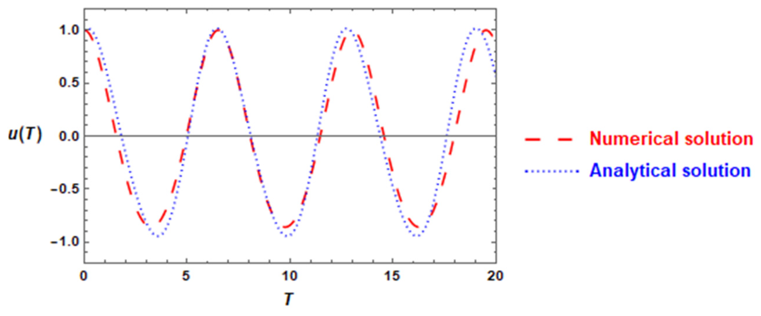
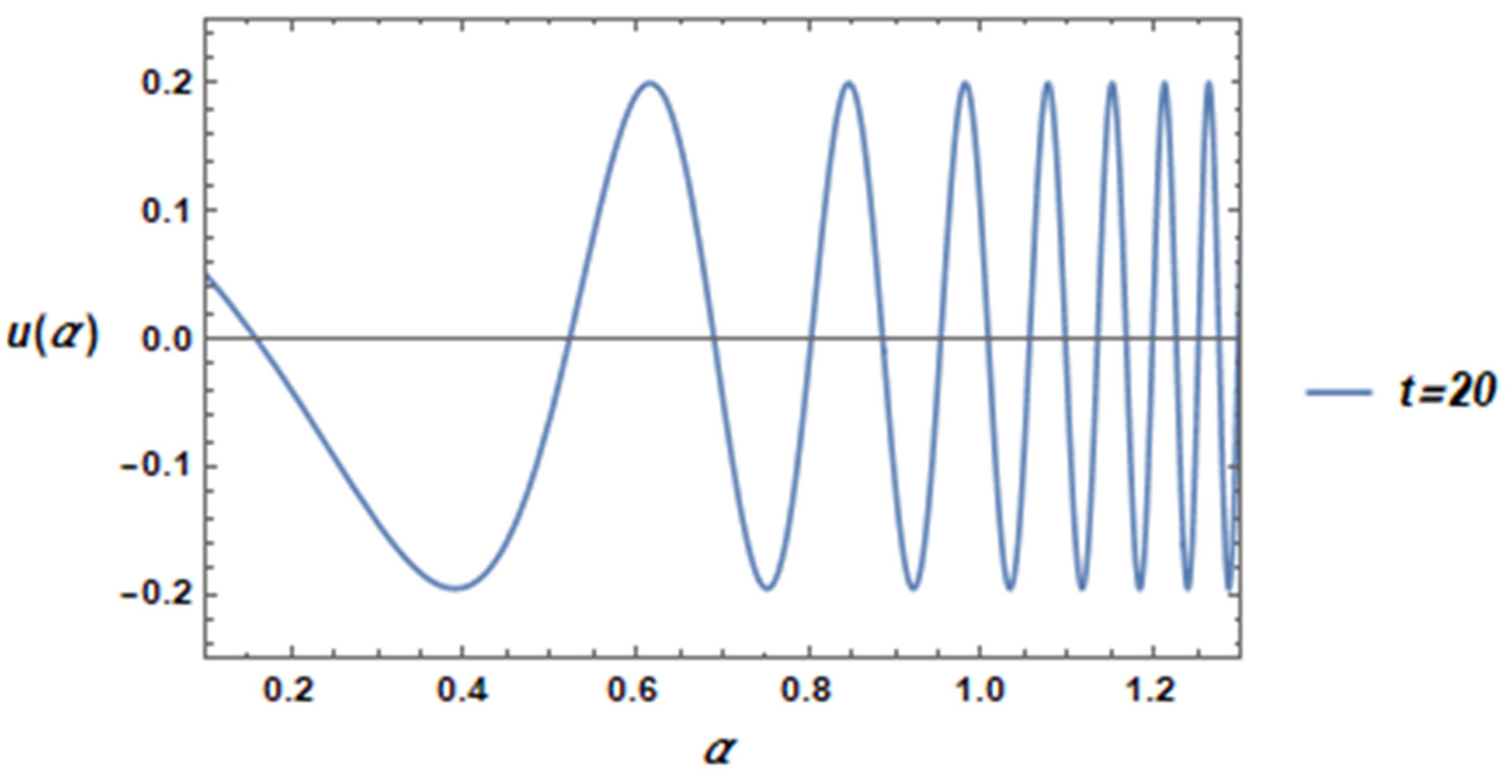
4. Numerical Illustration

For more opportunities, the attained approximate analytical solution must validate the numerical solution. For this perseverance, the numerical solution of Equation (21) was utilized to confirm the approximate solution (35). Therefore, Figure 1 is designed to demonstrate the bounded analytical solution given from the HPM, together with the numerical solution that is given by Mathematica software. Through this figure, the usage of the sample chosen system exposed that the value of the amplitude $A=0.1$ and $\alpha$ is supposed in the stander case of $\alpha =1$. As shown from this figure, the amplitudes of the solution in the two cases coincident. Additionally, both solutions behave in the periodic nature of the solution. It is found that there is excellent agreement between the analytical solution and the numerical solution even when the amplitude $A$ has increased, as displayed in Figure 2, Figure 3 and Figure 4. Three sequences of the parameter $\alpha$ are considered $\left(\alpha =0.6,0.8\&1\right)$ for the solution (35) with the fixed amplitude $A=0.2$ and graphed together in Figure 5. It is observed that an increase in $\alpha$ leads to a decrease in the wavelength with the wave height fixed. In Figure 6, the analytical solution (35) is plotted as a function of the parameter $\alpha$ with the fixed variable t to the value $t=20$. Again, an increase in the parameter $\alpha$ decreases the wavelength.

5. Conclusions

In this paper, we show the basic properties of a fractal oscillator in the frame of fractal variational theory. The fractal Tota oscillator can be obtained by minimizing the fractal variational formulation. The complexity of the Toda equation was relaxed by converting it to the jerk oscillator. The homotopy perturbation method was adopted to solve the nonlinear third-order differential equation, and the results are good enough for practical applications. The accuracy of the obtained solution was examined by comparing it with the numerical solutions which show excellent agreement even for relatively large amplitudes.

References

1. He, J.H. Variational principle and periodic solution of the Kundu–Mukherjee–Naskar equation. Results Phys. 2020, 17, 103031. [Google Scholar] [CrossRef]
2. He, J.H.; Anjum, N.; Skrzypacz, P.S. A Variational Principle for a Nonlinear Oscillator Arising in Microelectromechanical System. J. Appl. Comput. Mech. 2021, 7, 78–83. [Google Scholar] [CrossRef]
3. Liu, H.Y.; Li, Z.M.; Yao, S.W.; Yao, Y.J.; Liu, J. A variational principle for the photocatalytic NOx abatement. Therm. Sci. 2020, 24, 2515–2518. [Google Scholar] [CrossRef]
4. He, J.-H.; Hou, W.-F.; Qie, N.; Gepreel, K.A.; Shirazi, A.H.; Sedighi, H.M. Hamiltonian-based frequency-amplitude formulation for nonlinear oscillators. Facta Univ. Ser. Mech. Eng. 2021, 19, 199–208. [Google Scholar] [CrossRef]
5. He, J.H. The simpler, the better: Analytical methods for nonlinear oscillators and fractional oscillators. J. Low Freq. Noise Vib. Act. Control 2019, 38, 1252–1260. [Google Scholar] [CrossRef] [Green Version]
6. He, J.H. The simplest approach to nonlinear oscillators. Results Phys. 2019, 15, 102546. [Google Scholar] [CrossRef]
7. Cialdi, S.; Castelli, F.; Prati, F. Lasers as Toda oscillators: An experimental confirmation. Opt. Commun. 2013, 287, 76–179. [Google Scholar] [CrossRef]
8. Elías-Zúñiga, A.; Palacios-Pineda, L.M.; Jiménez-Cedeño, I.H.; Martínez-Romero, O.; Trejo, D.O. Equivalent power-form representation of the fractal Toda oscillator. Fractals 2021, 29, 2150034. [Google Scholar] [CrossRef]
9. Mboupda Pone, J.R.; Kingni, S.T.; Kol, G.R.; Pham, V.T. Hopf bifurcation, antimonotonicity and amplitude controls in the chotic Toda jerk oscillator: Analysis, circuit realization and combination synchronization in its fractional-order form. Automatika 2019, 60, 149–161. [Google Scholar] [CrossRef]
10. Takahashi, D.A. Newton’s equation of motion with quadratic drag force and Toda’s potential as a solvable one. Phys. Scr. 2018, 93, 075204. [Google Scholar] [CrossRef] [Green Version]
11. Tian, D.; Ain, Q.T.; Anjum, N. Fractal N/MEMS: From pull-in instability to pull-in stability. Fractals 2021, 29, 2050030. [Google Scholar] [CrossRef]
12. Tian, D.; He, C.H. A fractal micro-electromechanical system and its pull-in stability. J. Low Freq. Noise Vib. Act. Control 2021. [Google Scholar] [CrossRef]
13. Tian, D.; He, C.H.; He, J.H. Fractal Pull-in Stability Theory for Microelectromechanical Systems. Front. Phys.-Math. Stat. Phys. 2021, 9, 606011. [Google Scholar]
14. Ji, F.Y.; He, C.H.; Zhang, J.J.; He, J.H. A fractal Boussinesq equation for nonlinear transverse vibration of a nanofiber-reinforced concrete pillar. Appl. Math. Model. 2020, 82, 437–448. [Google Scholar] [CrossRef]
15. He, C.-H.; He, J.-H.; Sedighi, H.M. Fangzhu: An ancient Chinese nanotechnology for water collection from air: History, mathematical insight, promises, and challenges. Math. Methods Appl. Sci. 2021. [Google Scholar] [CrossRef]
16. Wang, K.L. Effect of Fangzhu’s nano-scale surface morphology on water collection. Math. Methods Appl. Sci. 2021. [Google Scholar] [CrossRef]
17. He, J.-H.; El-Dib, Y.O. Homotopy perturbation method for Fangzhu oscillator. J. Math. Chem. 2020, 58, 2245–2253. [Google Scholar] [CrossRef]
18. He, C.H.; Liu, C.; He, J.H.; Shirazi, A.H.; Mohammad-Sedighi, H. Passive Atmospheric water harvesting utilizing an ancient Chinese ink slab and its possible applications in modern architecture. Facta Univ. Mech. Eng. 2021, 19, 229–239. [Google Scholar] [CrossRef]
19. Wang, K.L. A new fractal model for the soliton motion in a microgravity space. Int. J. Numer. Methods Heat Fluid Flow. 2020. [Google Scholar] [CrossRef]
20. Zuo, Y.-T. A gecko-like fractal receptor of a three-dimensional printing technology: A fractal oscillator. J. Math. Chem. 2021, 59, 735–744. [Google Scholar] [CrossRef]
21. Elias-Zuniga, A.; Palacios-Pineda, L.M.; Jiménez-Cedeño, I.H.; Martínez-Romero, O.; Olvera-Trejo, D. A fractal model for current generation in porous electrodes. J. Electroanal. Chem. 2021, 880, 114883. [Google Scholar] [CrossRef]
22. Elias-Zuniga, A.; Palacios-Pineda, L.M.; Jimenez-Cedeno, I.H.; Martínez-Romeroa, O.; Olvera-Trejo, D. Analytical solution of the fractal Cubic-Quintic Duffing equation. Fractals 2021, 29, 2150080. [Google Scholar] [CrossRef]
23. He, C.H.; Liu, C.; Gepreel, K.A. Low frequency property of a fractal vibration model for a concrete beam. Fractals 2021, 29, 2150117. [Google Scholar] [CrossRef]
24. He, C.H.; Liu, C.; He, J.H.; Mohammad-Sedighi, H.; Shokri, A.; Gepreel, K.A. A fractal model for the internal temperature response of a porous concrete. Appl. Comput. Math. 2021, 20, 1871–1875. [Google Scholar]
25. Wang, K.L.; Wei, C.F. A powerful and simple frequency formula to nonlinear fractal oscillators. J. Low Freq. Noise Vib. Act. Control 2020. [Google Scholar] [CrossRef]
26. Elías-Zúñiga, A.; Palacios-Pineda, L.M.; Jiménez-Cedeño, I.H.; Martínez-Romero, O.; Trejo, D.O. He’s frequency–amplitude formulation for nonlinear oscillators using Jacobi elliptic functions. J. Low Freq. Noise Vib. Act. Control 2020, 39, 1216–1223. [Google Scholar] [CrossRef]
27. He, J.H.; Kou, S.J.; He, C.H.; Zhang, Z.W.; Gepreel, K.A. Fractal oscillation and its frequency-amplitude property. Fractals 2021, 29, 2150105. [Google Scholar] [CrossRef]
28. Feng, G.Q. He’s frequency formula to fractal undamped Duffing equation. J. Low Freq. Noise Vib. Act. Control 2021. [Google Scholar] [CrossRef]
29. He, J.H.; Qie, N.; He, C.H.; Saeed, T. On a strong minimum condition of a fractal variational principle. Appl. Math. Lett. 2021, 119, 107199. [Google Scholar] [CrossRef]
30. He, J.H.; Ain, Q.T. New promises and future challenges of fractal calculus: From two-scale thermodynamics to fractal variational principle. Therm. Sci. 2020, 24, 659–681. [Google Scholar] [CrossRef]
31. He, J.H. A fractal variational theory for one-dimensional compressible flow in a microgravity space. Fractals 2020, 28, 2050024. [Google Scholar] [CrossRef]
32. He, J.H. On the fractal variational principle for the Telegraph equation. Fractals 2021, 29, 2150022. [Google Scholar] [CrossRef]
33. Wang, K.L.; Yao, S.W. Fractal variational theory for Chaplygin-He Gas in a microgravity condition. Comput. Methods Appl. Mech. Eng. 2020, 6, 1606–1612. [Google Scholar]
34. Wang, K.L.; He, C.H. A remark on Wang’s fractal variational principle. Fractals 2019, 27, 1950134. [Google Scholar] [CrossRef]
35. Khan, Y. A novel soliton solutions for the fractal Radhakrishnan-Kundu-Lakshmanan model arising in birefringent fibers. Opt. Quantum Electron. 2021, 53, 127. [Google Scholar] [CrossRef]
36. Khan, Y. Fractal modification of complex Ginzburg-Landau model arising in the oscillating phenomena. Results Phys. 2020, 18, 103324. [Google Scholar] [CrossRef]
37. Khan, Y. A variational approach for novel solitary solutions of FitzHugh-Nagumo equation arising in the nonlinear reac-tion-diffusion equation. Int. J. Numer. Methods Heat Fluid Flow 2020, 31. [Google Scholar] [CrossRef]
38. Cao, X.Q.; Hou, S.C.; Guo, Y.N.; Zhang, C.Z.; Peng, K.C. Variational principle for 2+1 dimensional Broer-Kaup equations with fractal derivatives. Fractals 2020, 28, 2050107. [Google Scholar] [CrossRef]
39. He, J.H.; El-Dib, Y.O. The reducing rank method to solve third-order Duffing equation with the homotopy perturbation. Numer. Methods Partial. Differ. Equ. 2020, 37, 1800–1808. [Google Scholar] [CrossRef]
40. He, J.H. Homotopy perturbation technique. Comput. Methods Appl. Mech. Eng. 1999, 178, 257–262. [Google Scholar] [CrossRef]
41. He, J.H.; El-Dib, Y.O. Homotopy perturbation method with three expansions. J. Math. Chem. 2021, 59, 1139–1150. [Google Scholar] [CrossRef]
42. He, J.H.; El-Dib, Y.O. Periodic property of the time-fractional Kundu–Mukherjee–Naskar equation. Results Phys. 2020, 19, 103345. [Google Scholar] [CrossRef]
43. Li, X.X.; He, C.H. Homotopy perturbation method coupled with the enhanced perturbation method. J. Low Freq. Noise Vib. Act. Control 2019, 38, 1399–1403. [Google Scholar] [CrossRef]
44. Ji, Q.P.; Wang, J.; Lu, L.X.; Ge, C.F. Li-He’s modified homotopy perturbation method coupled with the energy method for the dropping shock response of a tangent nonlinear packaging system. J. Low Freq. Noise Vib. Act. Control 2020, 40, 675–682. [Google Scholar] [CrossRef]
45. Shen, Y.; El-Dib, Y.O. A periodic solution of the fractional sine-Gordon equation arising in architectural engineering. J. Low-Freq. Noise. Vib. Act. Control 2020. [Google Scholar] [CrossRef] [Green Version]
46. El-Dib, Y.O.; Elgazery, N. Effect of fractional derivative properties on the periodic solution of the nonlinear oscillators. Fractals 2020, 28, 2050095. [Google Scholar] [CrossRef]
47. El-Dib, Y.O. Homotopy perturbation method with rank upgrading technique for the superior nonlinear oscillation. Math. Comput. Simul. 2021, 182, 555–565. [Google Scholar] [CrossRef]
48. El-Dib, Y.O.; Matoog, R.T. The Rank Upgrading Technique for a Harmonic Restoring Force of Nonlinear oscillators. Appl. Comput. Mech. 2021, 7, 782–789. [Google Scholar]
Figure 1. Comparison between the numerical solution (dashed red line) of the Toda Equation (21) and the analytical solution (dotted blue line) of the solution (35) in the case of α = 1 .
Fractalfract 05 00093 g001
Figure 2. Comparison between the numerical solution (dashed red line) of the Toda Equation (21) and the analytical solution (dotted blue line) of the solution (35) in the case of α = 1 .
Fractalfract 05 00093 g002
Figure 3. Comparison between the numerical solution (dashed red line) of the Toda Equation (21) and the analytical solution (dotted blue line) of the solution (35) in the case of α = 1 .
Fractalfract 05 00093 g003
Figure 4. Comparison between the numerical solution (dashed red line) of the Toda Equation (21) and the analytical solution (dotted blue line) of the solution (35) in the case of α = 1 .
Fractalfract 05 00093 g004
Figure 5. Graphing the solution (35) for sequences of the parameter α .
Fractalfract 05 00093 g005
Figure 6. Plots the approximate solution (35) as a function in α .
Fractalfract 05 00093 g006
Publisher’s Note: MDPI stays neutral with regard to jurisdictional claims in published maps and institutional affiliations.