
Analytic Fuzzy Formulation of a Time-Fractional Fornberg–Whitham Model with Power and Mittag–Leffler Kernels

 ,
,  and
and 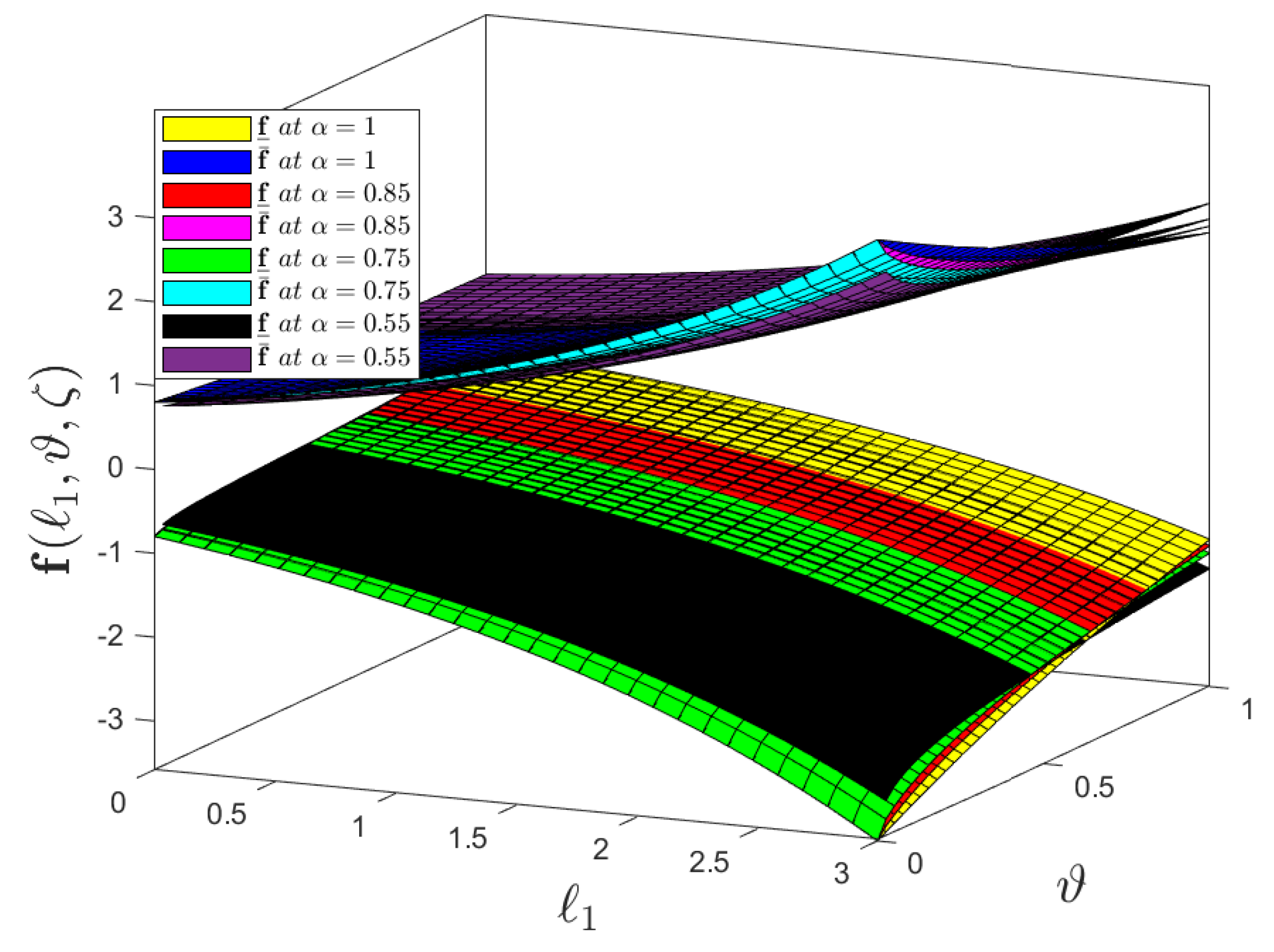
Abstract
1. Introduction
2. Preliminaries
- 1.
- Ω is normal (for some );
- 2.
- Ω is upper semi continuous;
- 3.
- , i.e., Ω is convex;
- 4.
- is compact.
- 1.
- is non-decreasing, left continuous, bounded over and left continuous at
- 2.
- is non-increasing, right continuous, bounded over and right continuous at
- 3.
- 1.
- 2.
- 3.
- (i)
- .
- (ii)
- (i)
- For all of sufficiently small size, the subsequent -differences exist:and the following limits hold:
- (ii)
- For all of sufficiently small size, the subsequent -differences exist:and the following limits hold:
- (i)
- If is -partial differentiable for ℓ (i.e., Θ is partial differentiable for ℓ under the meaning of Definition 8(i)), then
- (ii)
- If is -partial differentiable for ℓ (i.e., Θ is partial differentiable for ℓ under the meaning of Definition 8(ii)), then
2.1. A Fuzzy Elzaki Transform for Fuzzy Caputo Fractional Derivative and a Fuzzy Atangana–Baleanu Fractional Derivative Operator
2.2. Some Algebraic Properties of Fuzzy Elzaki Transform
3. Proposed Algorithm
4. Test Examples and Their Physical Interpretation
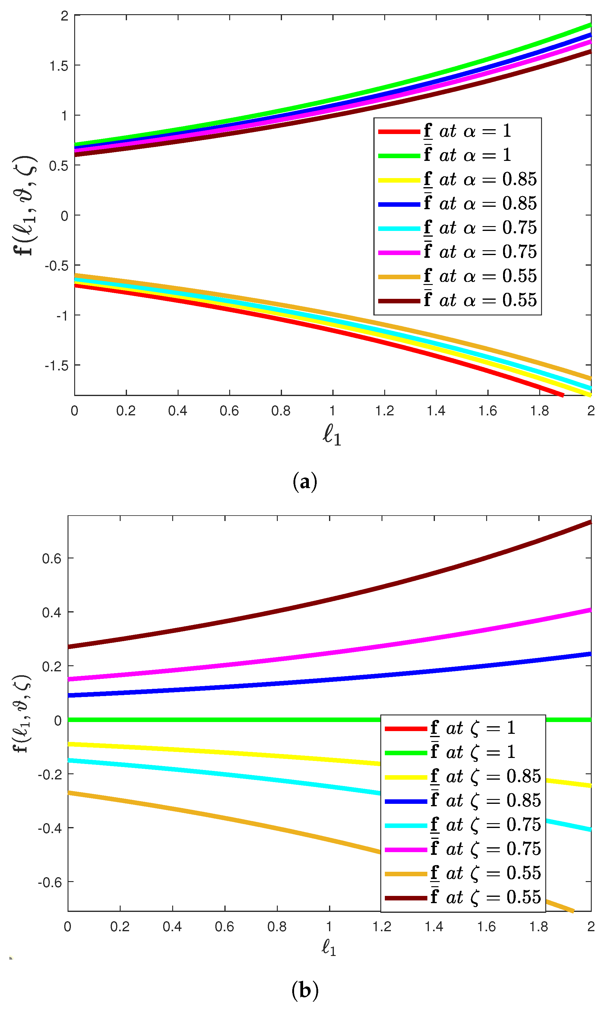
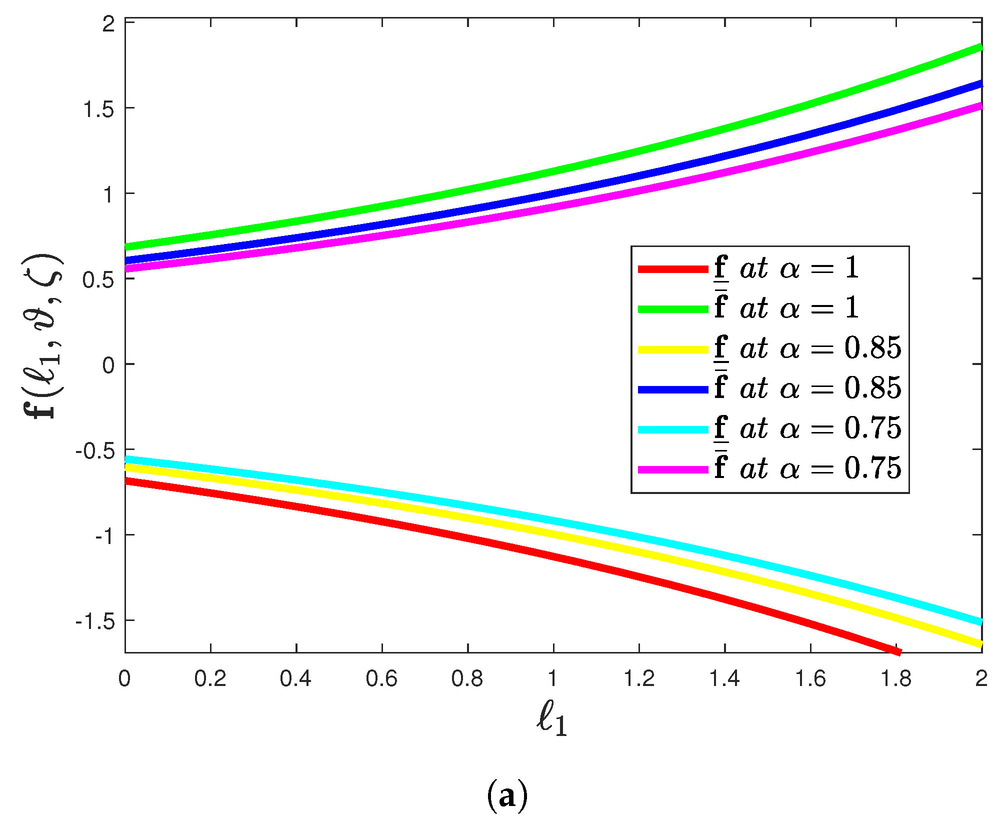
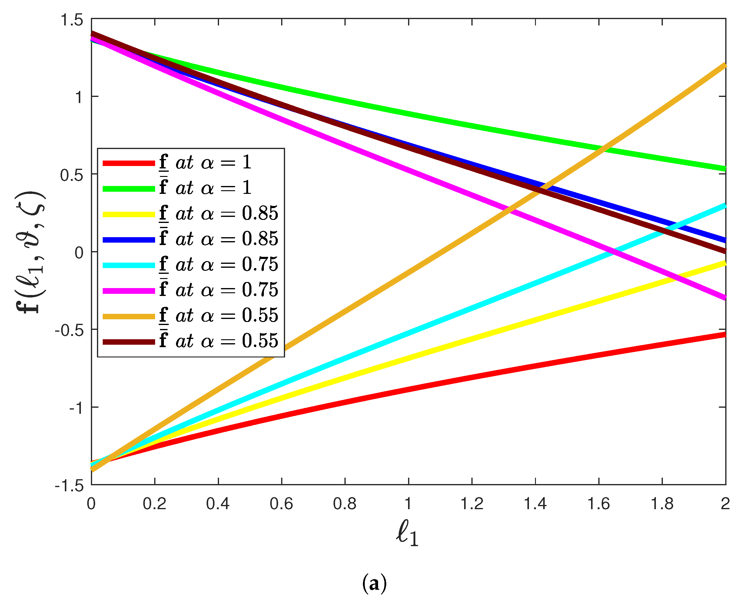
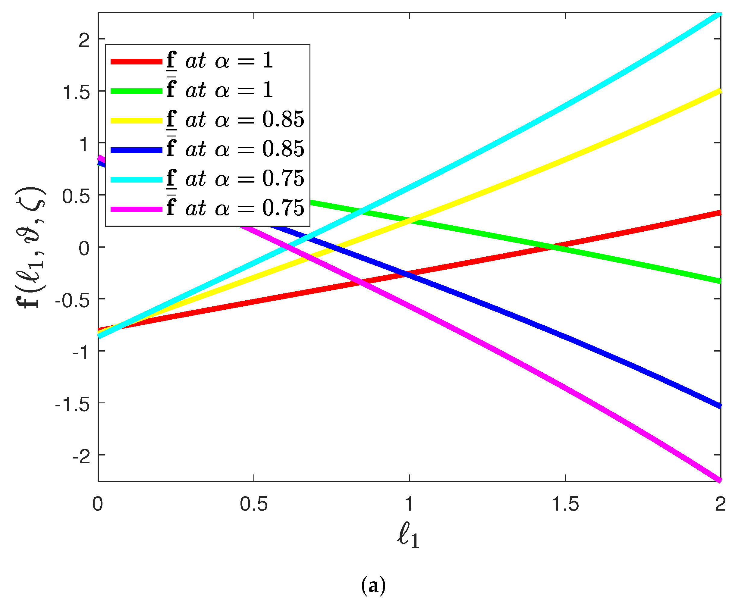
- The effect of the proposed methodology on the mapping is displayed in Figure 2a for the varying fractional orders by considering CFD operator. It exhibits a relatively small increase in the mapping with the decrease in .
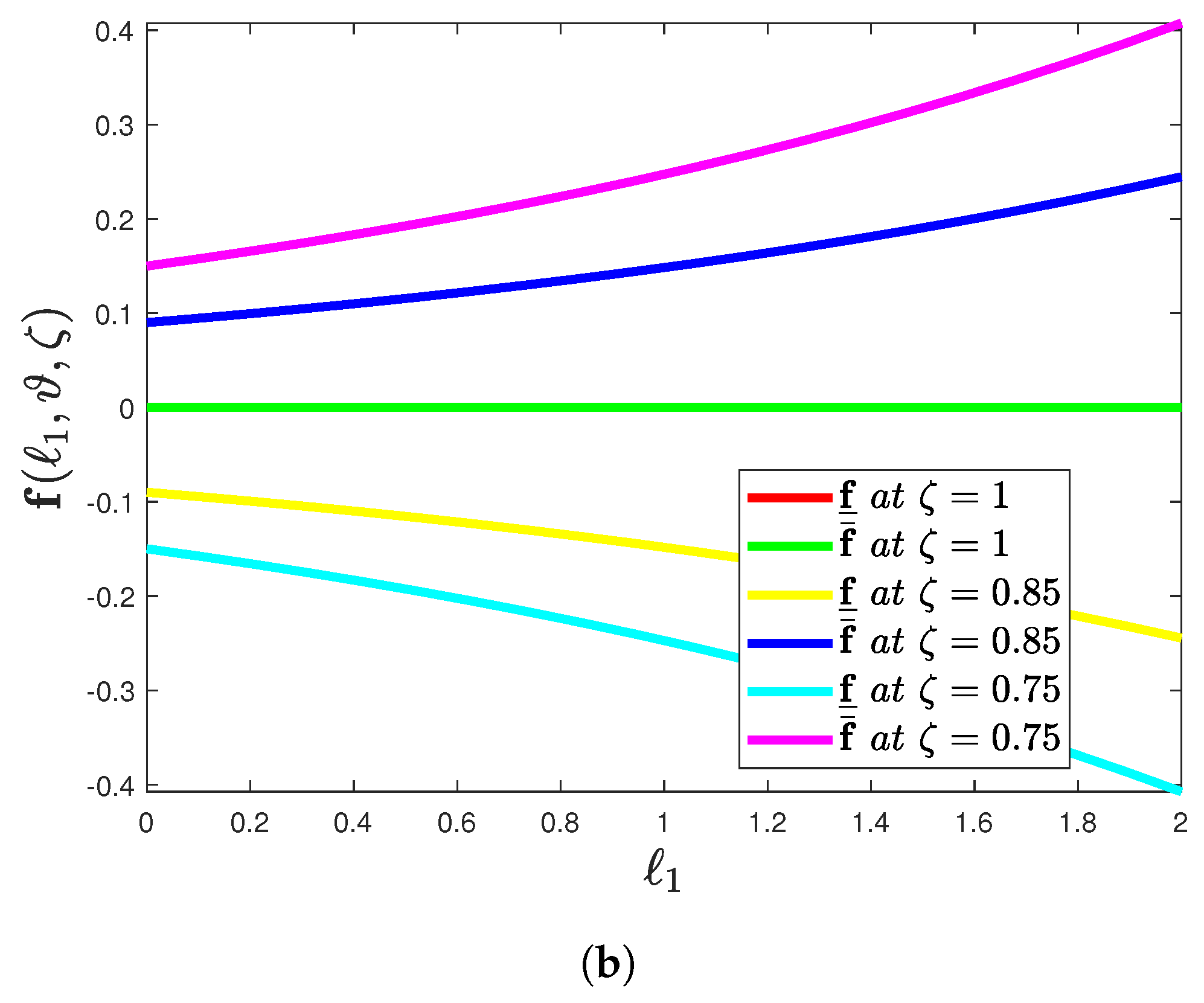
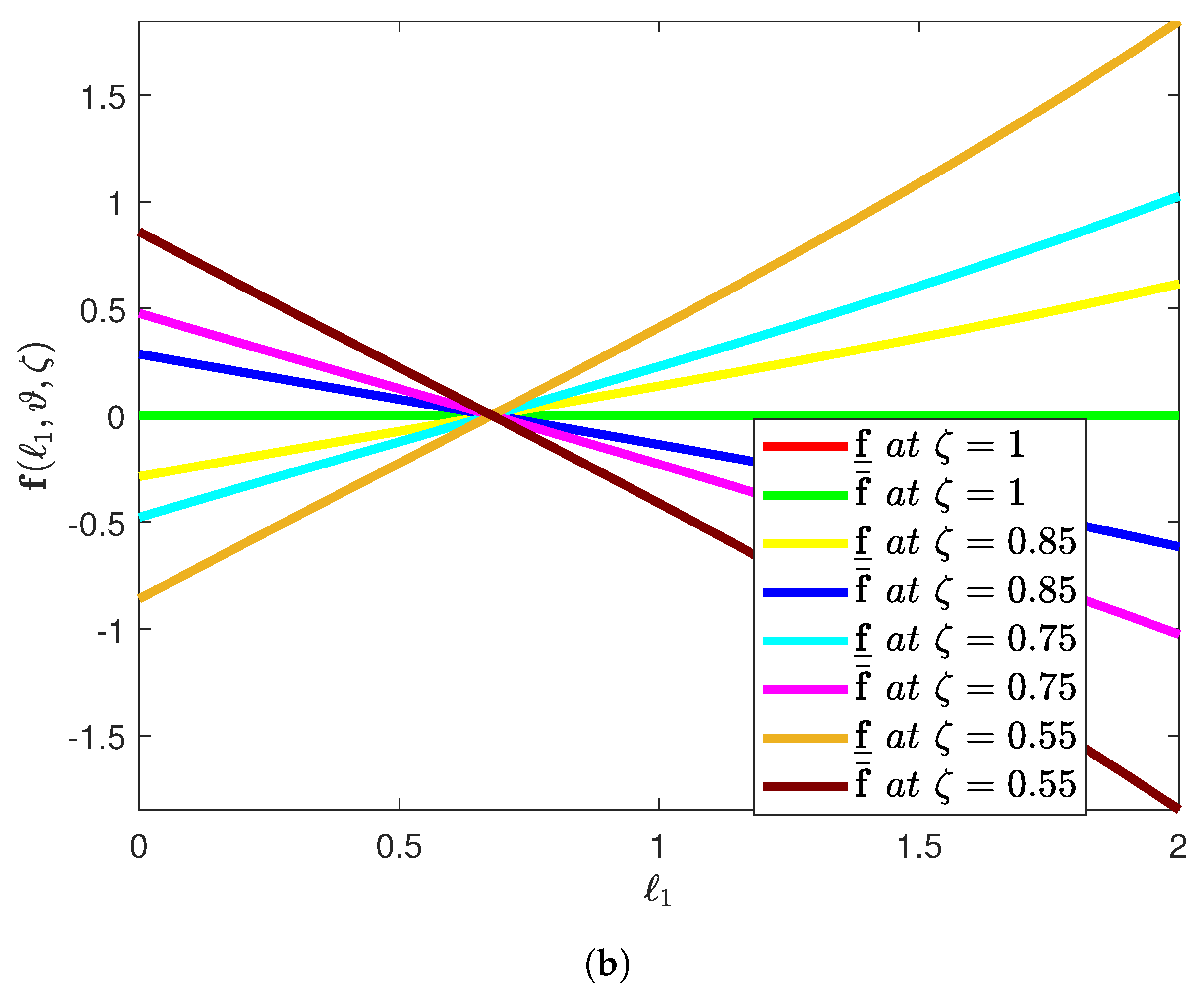
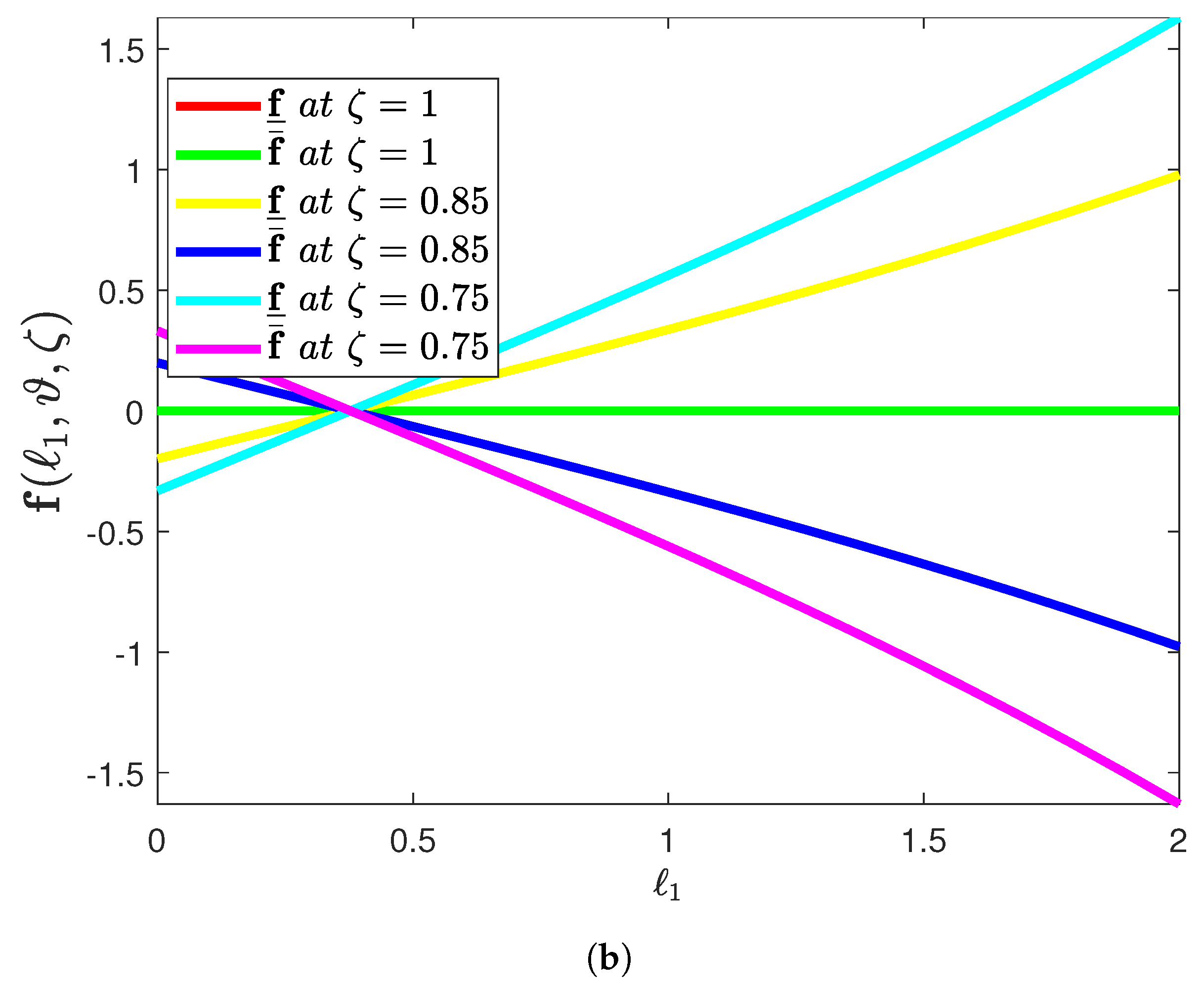
- The profile graph of Figure 2b demonstrates the lower and upper solution of varying uncertainty when the fractional order is assumed to be by proposing CFD operator. It emphasizes a relatively small variation in the mapping with the increase in .
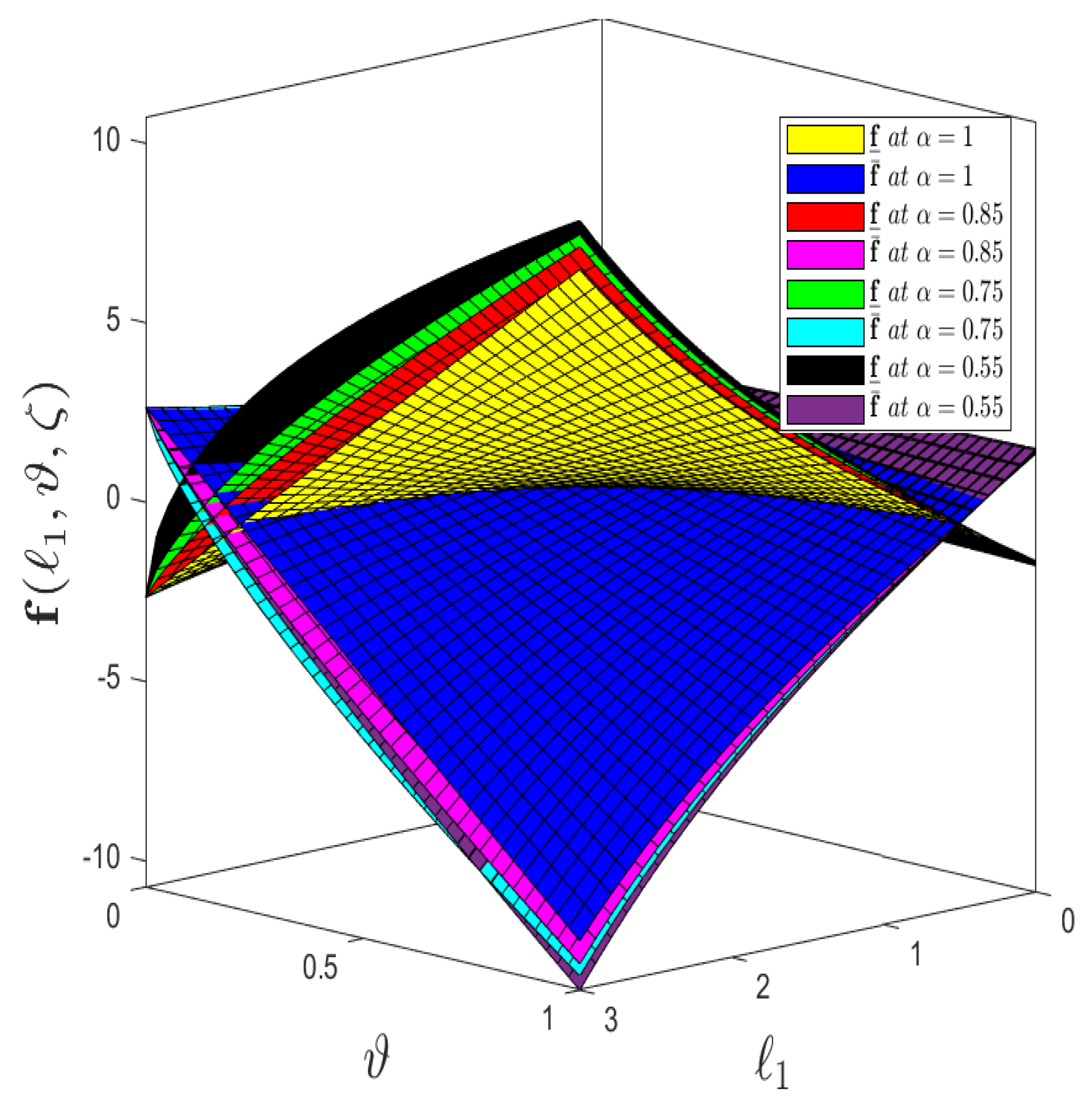
- The effect of the proposed methodology on the mapping is displayed in Figure 3a for the varying fractional orders by considering the ABC fractional derivative operator. It exhibits a relatively small increase in the mapping with the decrease in .
- The Profile graph of Figure 3b demonstrates the lower and upper solutions of varying uncertainty when the fractional order is assumed to be by proposing the ABC fractional derivative operator. It emphasizes a relatively small variation in the mapping with the increase in .
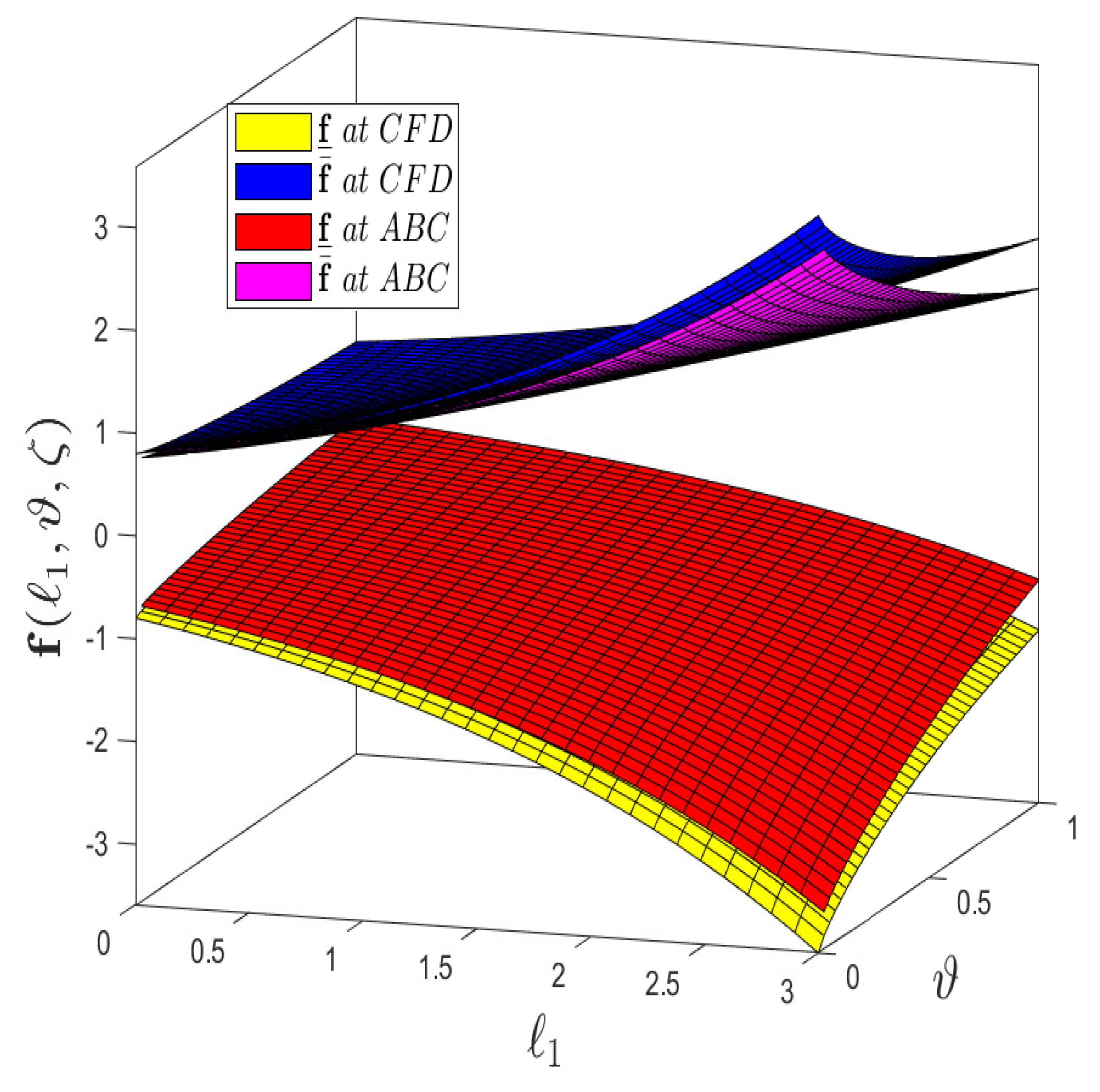
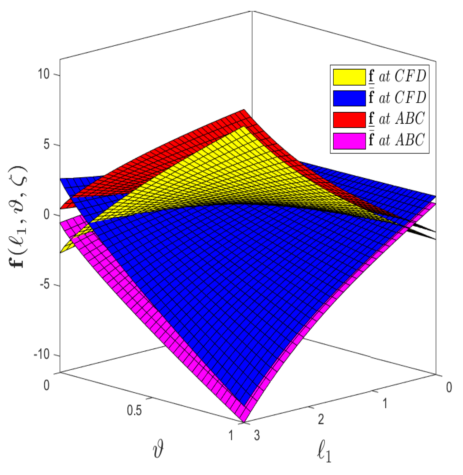
- Figure 4 demonstrates the comparison analysis between the CFD operator and the ABC fractional derivative operator for varying fractional order with uncertainty exhibits that lower the solution profile for the ABC fractional operator has strong ties with the upper solution as compared to the CFD operator.
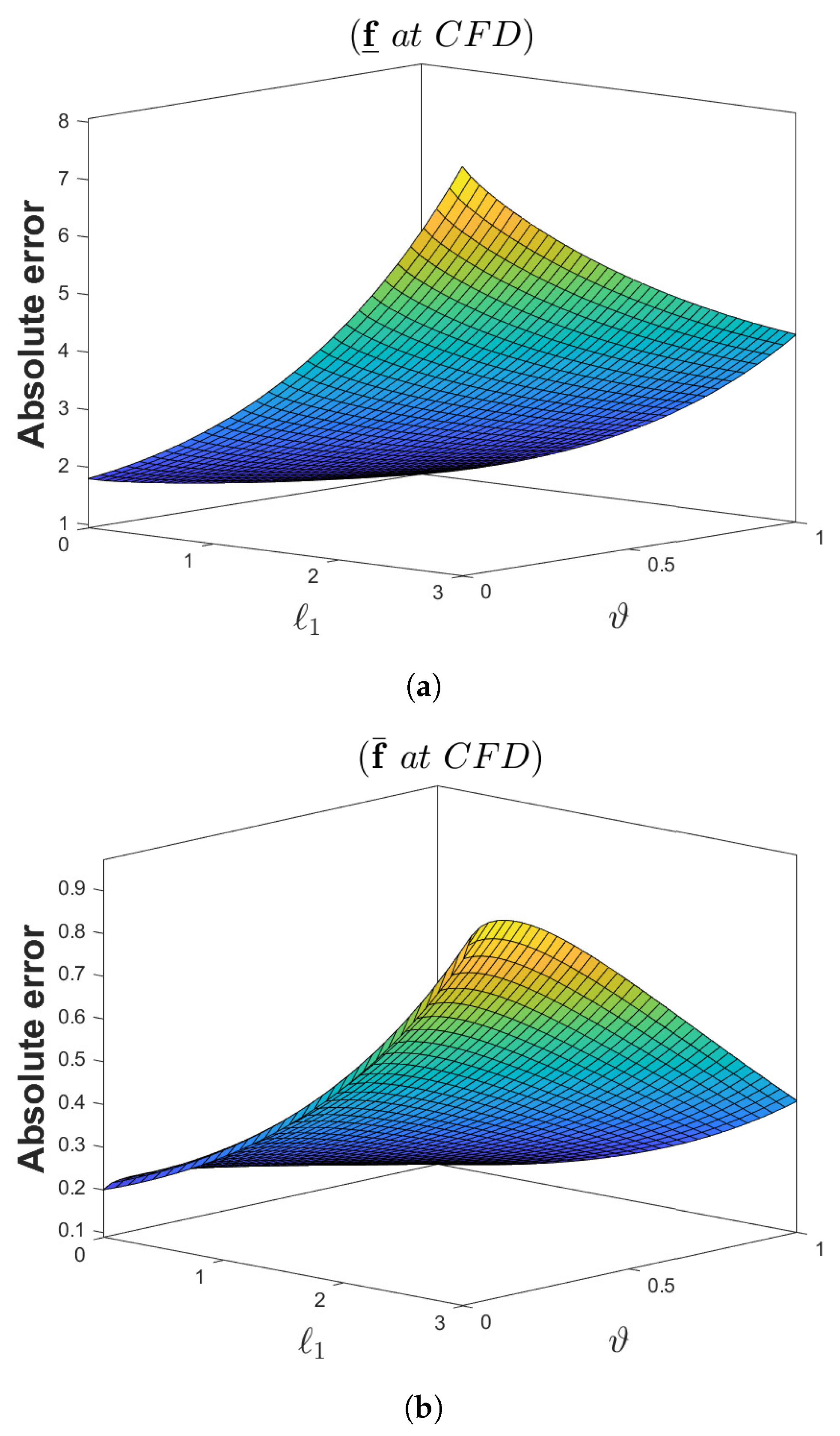
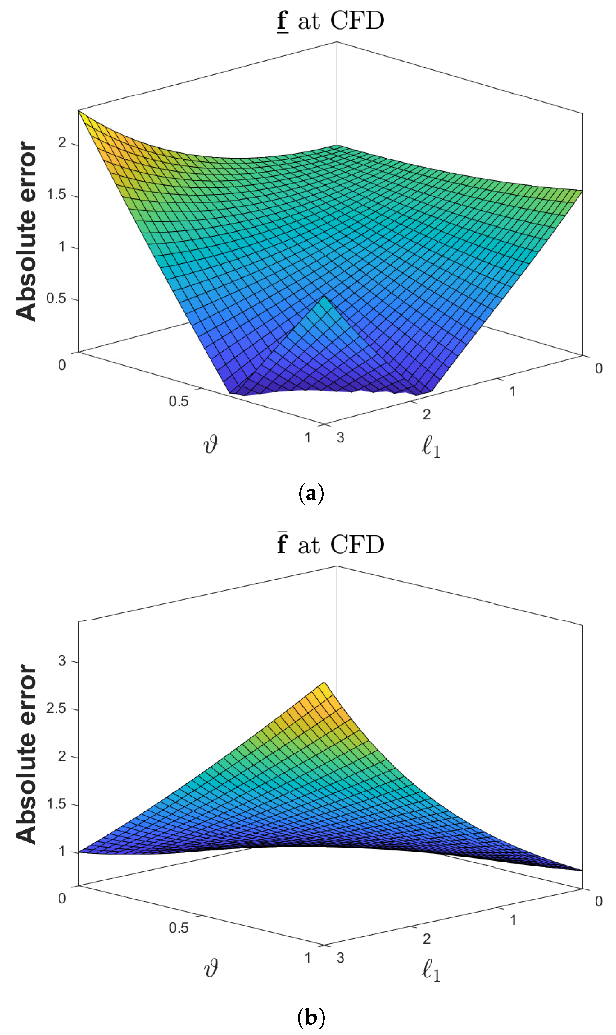
- Figure 5 shows the comparison analysis between ( and the exact solution), ( and exact solution), respectively, for three dimensional error plots by considering the CFD operator.
- The effect of the proposed methodology on the mapping is displayed in Figure 7a for the varying fractional-orders by the considering CFD operator. It exhibits a relatively small increase in the mapping with the decrease in .
- The profile graph of Figure 7b demonstrates the lower and upper solution of varying uncertainty when the fractional order is assumed to be by proposing the CFD operator. It emphasizes a relatively small variation in the mapping with the increase in .
- The effect of the proposed methodology on the mapping is displayed in Figure 8a for the varying fractional orders by considering ABC fractional derivative operator. It exhibits a relatively small increase in the mapping with the decrease in .
- The profile graph of Figure 8b demonstrates the lower and upper solutions of varying uncertainty when the fractional order is assumed to be by proposing the ABC fractional derivative operator. It emphasizes a relatively small variation in the mapping with the increase in .
- Figure 9 demonstrates the comparison analysis between CFD operator and ABC fractional derivative operator for varying fractional order with uncertainty exhibits that the lower solution profile for ABC fractional operator has strong ties with the upper solution as compared to the CFD operator.
- Figure 10 shows the comparison analysis between ( and the exact solution), ( and the exact solution), respectively, for three dimensional error plots by considering the CFD operator.
5. Conclusions
Author Contributions
Funding
Institutional Review Board Statement
Informed Consent Statement
Data Availability Statement
Acknowledgments
Conflicts of Interest
References
- Podlubny, I. Fractional Differential Equations; Academic Press: San Diego, CA, USA, 1999. [Google Scholar]
- Hilfer, R. Applications of Fractional Calculus in Physics; Word Scientific: Singapore, 2000. [Google Scholar]
- Kilbas, A.; Srivastava, H.M.; Trujillo, J.J. Theory and Application of Fractional Differential Equations; Elsevier: Amsterdam, The Netherlands, 2006; Volume 204, pp. 1–523. [Google Scholar]
- Magin, R.L. Fractional Calculus in Bioengineering; Begell House Publishers: Redding, CT, USA, 2006. [Google Scholar]
- Samko, S.G.; Kilbas, A.A.; Marichev, O.I. Fractional Integrals and Derivatives: Theory and Applications; Gordon and Breach Science Publishers: Philadelphia, PA, USA, 1993. [Google Scholar]
- Jajarmi, A.; Baleanu, D. On the fractional optimal control problems with a general derivative operator. Asian J. Cont. 2021, 23, 1062–1071. [Google Scholar] [CrossRef]
- Jajarmi, A.; Baleanu, D. Suboptimal control of fractional-order dynamic systems with delay argument. J. Vib. Control 2018, 24, 2430–2446. [Google Scholar] [CrossRef]
- Baleanu, D.; Zibaei, S.; Namjoo, M.; Jajarmi, A. A nonstandard finite difference scheme for the modeling and nonidentical synchronization of a novel fractional chaotic system. Adv. Diff. Eqs. 2021, 2021, 308. [Google Scholar] [CrossRef]
- Tuan, N.H.; Ganji, R.M.; Jafari, H. A numerical study of fractional rheological models and fractional Newell-Whitehead-Segel equation with non-local and non-singular kernel. Chin. J. Phys. 2020, 68, 308–320. [Google Scholar] [CrossRef]
- Ganji, R.M.; Jafari, H.; Baleanu, D. A new approach for solving multi variable orders differential equations with Mittag–Leffler kernel. Chaos Solitons Fract. 2020, 130, 109405. [Google Scholar] [CrossRef]
- Baleanu, D.; Jajarmi, A.; Mohammadi, H.; Rezapour, S. A new study on the mathematical modelling of human liver with Caputo–Fabrizio fractional derivative. Chaos Solitons Fract. 2020, 134, 109705. [Google Scholar] [CrossRef]
- Rashid, S.; Khalid, A.; Bazighifan, O.; Oros, G.I. New modifications of integral inequalities via ℘-convexity pertaining to fractional calculus and their applications. Mathematics 2021, 9, 1753. [Google Scholar] [CrossRef]
- Atangana, A.; Baleanu, D. New fractional derivatives with nonlocal and non-singular kernel: Theory and application to heat transfer model. Therm. Sci. 2016, 20, 763–769. [Google Scholar] [CrossRef]
- Caputo, M.; Fabrizio, M. A new definition of fractional derivative without singular kernel. Prog. Fract. Differ. Appl. 2015, 1, 1–13. [Google Scholar]
- Baleanu, D.; Sajjadi, S.S.; Jajarmi, A.; Defterli, O. On a nonlinear dynamical system with both chaotic and non-chaotic behaviours: A new fractional analysis and control. Adv. Differ. Equ. 2021, 2021, 234. [Google Scholar] [CrossRef]
- Abdeljawad, T.; Baleanu, D. Integration by parts and its applications of a new nonlocal fractional derivative with Mittag-Leffler nonsingular kernel. Nonlinear Anal. Theory Methods Appl. 2017, 10, 1098–1107. [Google Scholar] [CrossRef]
- Abdeljawad, T. Fractional operators with generalized Mittag-Leffler kernels and their iterated differintegrals. Chaos 2019, 29, 023102. [Google Scholar] [CrossRef]
- Li, Z.; Wang, C.; Agarwal, R.P.; Sakthivel, R. Hyers-Ulam-Rassias stability of quaternion multidimensional fuzzy nonlinear difference equations with impulses. Iran. J. Fuzzy Syst. 2021, 18, 143–160. [Google Scholar]
- Kandel, A.; Byatt, W.J. Fuzzy differential equations. In Proceedings of the International Conference Cybernetics and Society, Tokyo, Japan, 3–7 November 1978; pp. 1213–1216. [Google Scholar]
- Agarwal, R.P.; Lakshmikantham, V.; Nieto, J.J. On the concept of solution for fractional differential equations with uncertainty. Nonlin. Anal. Theory Meth Appl. 2010, 72, 2859–2862. [Google Scholar] [CrossRef]
- El-Sayed, S.; Kaya, D. An application of the ADM to seven-order Sawada-Kotara equations. Appl. Math. Comput. 2004, 157, 93–101. [Google Scholar] [CrossRef]
- El-Tawil, M.A.; Huseen, S. On convergence of the q-homotopy analysis method. Int. J. Contemp. Math. Sci. 2013, 8, 481–497. [Google Scholar] [CrossRef]
- Darvishia, M.T.; Kheybaria, S.; Khanib, F. A numerical solution of the Lax’s 7th-order KdV equation by Pseudo spectral method and Darvishi’s Preconditioning. Int. J. Contemp. Math. Sci. 2007, 2, 1097–1106. [Google Scholar] [CrossRef]
- Shiralashetti, S.C.; Kumbinarasaiah, S. Laguerre wavelets collocation method for the numerical solution of the Benjamina–Bona–Mohany equations. J. Taibah Univ. Sci. 2019, 13, 9–15. [Google Scholar] [CrossRef]
- Lahmar, N.A.; Belhamitib, O.; Bahric, S.M. A new Legendre-Wavelets decomposition method for solving PDEs. Malaya J. Mat. 2014, 1, 72–81. [Google Scholar]
- Hoa, N.V.; Vu, H.; Duc, T.M. Fuzzy fractional differential equations under Caputo Katugampola fractional derivative approach. Fuzzy Sets Syst. 2019, 375, 70–99. [Google Scholar] [CrossRef]
- Hoa, N.V. Fuzzy fractional functional differential equations under Caputo gH-differentiability. Commun. Nonlinear Sci. Numer. Simul. 2015, 22, 1134–1157. [Google Scholar] [CrossRef]
- Salahshour, S.; Ahmadian, A.; Senu, N.; Baleanu, D.; Agarwal, P. On analytical aolutions of the fractional differential equation with uncertainty: Application to the Basset problem. Entropy 2015, 17, 885–902. [Google Scholar] [CrossRef]
- Ahmad, S.; Ullah, A.; Akgül, A.; Abdeljawad, T. Semi-analytical solutions of the 3rd order fuzzy dispersive partial differential equations under fractional operators. Alex. Eng. J. 2021, 60, 5861–5878. [Google Scholar] [CrossRef]
- Shah, K.; Seadawy, A.R.; Arfan, M. Evaluation of one dimensional fuzzy fractional partial differential equations. Alex. Eng. J. 2020, 59, 3347–3353. [Google Scholar] [CrossRef]
- Allahviranloo, T. An analytic approximation to the solution of fuzzy heat equation by Adomian decomposition method. Int. J. Contemp. Math. Sci. 2009, 4, 105–114. [Google Scholar]
- Allahviranloo, T. The Adomian decomposition method for fuzzy system of linear equations. Appl. Math. Comput. 2005, 163, 553–563. [Google Scholar] [CrossRef]
- Biswas, S.; Roy, T.K. Adomian decomposition method for fuzzy differential equations with linear differential operator. J. Comput. Inf. Sci. Eng. 2016, 11, 243–250. [Google Scholar]
- Hamoud, A.; Ghadle, K. Modified Adomian decomposition method for solving fuzzy Volterra–Fredholm integral equations. J. Indian Math. Soc. 2018, 85, 52–69. [Google Scholar]
- Whitham, G.B. Variational methods and applications to water wave. Proc. R. Soc. Lond. Ser. A 1967, 299, 6–25. [Google Scholar]
- Fornberg, B.; Whitham, G.B. A numerical and theoretical study of certain nonlinear wave phenomena. Philos. Trans. R. Soc. Lond. Ser. A 1978, 289, 373–404. [Google Scholar]
- Abidi, F.; Omrani, K. The homotopy analysis method for solving the Fornberg—Whitham equation and comparison with Adomian’s decomposition method. Comput. Math. Appl. 2010, 59, 2743–2750. [Google Scholar] [CrossRef]
- Gupta, P.K.; Singh, M. Homotopy perturbation method fractional Fornberg–Whitham equation. Comput. Math. Appl. 2011, 61, 250–254. [Google Scholar] [CrossRef]
- Lu, J. An analytical approach to the Fornberg–Whitham type equations by using the variational iteration method. Comput. Math. Appl. 2011, 61, 2010–2013. [Google Scholar] [CrossRef][Green Version]
- Sakar, M.G.; Erdogan, F.; Yildirim, A. Variational iteration method for the time-fractional Fornberg–Whitham equation. Comput. Math. Appl. 2012, 63, 1382–1388. [Google Scholar] [CrossRef]
- Chen, A.; Li, J.; Deng, X.; Huang, W. Travelling wave solutions of the Fornberg–Whitham equation. Appl. Math. Comput. 2009, 215, 3068–3075. [Google Scholar]
- Yin, J.; Tian, L.; Fan, X. Classification of travelling waves in the Fornberg–Whitham equation. J. Math. Anal. Appl. 2010, 368, 133–143. [Google Scholar] [CrossRef]
- Zhou, J.; Tian, L. A type of bounded traveling wave solutions for the Fornberg–Whitham equation. J. Math. Anal. Appl. 2008, 346, 255–261. [Google Scholar] [CrossRef]
- He, B.; Meng, Q.; Li, S. Explicit peakon and solitary wave solutions for the modified Fornberg–Whitham equation. Appl. Math. Comput. 2010, 5, 1976–1982. [Google Scholar] [CrossRef]
- Fan, X.; Yang, S.; Yin, J.; Tian, L. Bifurcations of traveling wave solutions for a two-component Fornberg–Whitham equation. Commun. Nonlinear Sci. Numer. Simul. 2011, 16, 3956–3963. [Google Scholar] [CrossRef]
- Jiang, B.; Bi, B. Smooth and non-smooth traveling wave solutions of the Fornberg–Whitham equation with linear dispersion term. Appl. Math. Comput. 2010, 216, 2155–2162. [Google Scholar] [CrossRef]
- Adomian, G. A review of the decomposition method in applied mathematics. J. Math. Anal. Appl. 1988, 135, 501–544. [Google Scholar] [CrossRef]
- Belgacem, F.B.M.; Karaballi, A.A.; Kalla, S.L. Analytical investigations of the sumudu transform and applications to integral production equations. Math. Prob. Eng. 2003, 2003, 103–118. [Google Scholar] [CrossRef]
- Aboodh, K.S. The new integral transform “Aboodh Transform”. Glob. J. Pure Appl. Math. 2013, 9, 35–43. [Google Scholar]
- Elzaki, T.M. Application of new transform Elzaki transform to partial differential equations. Glob. J. Pure Appl. Math. 2011, 7, 65–70. [Google Scholar]
- Mahgoub, M.M.A. The new integral transform “Mohand Transform”. Adv. Theor. Appl. Math. 2017, 12, 113–120. [Google Scholar]
- Rashid, S.; Hammouch, Z.; Aydi, H.; Ahmad, A.G.; Alsharif, A.M. Novel computations of the time-fractional Fisher’s model via generalized fractional integral operators by means of the Elzaki transform. Fractal Fract. 2021, 5, 94. [Google Scholar] [CrossRef]
- Rashid, S.; Kubra, K.T.; Guirao, J.L.G. Construction of an approximate analytical solution for multi-dimensional fractional Zakharov-Kuznetsov equation via Aboodh adomian decomposition method. Symmetry 2021, 13, 1542. [Google Scholar] [CrossRef]
- Rashid, S.; Kubra, K.T.; Abualnaja, K.M. Fractional view of heat-like equations via the Elzaki transform in the settings of the Mittag-Leffler function. Math. Methods Appl. Sci. 2021. [Google Scholar] [CrossRef]
- Rashid, S.; Khalid, A.; Sultana, S.; Hammouch, Z.; Shah, R.; Alsharif, A.M. A novel analytical view of time-fractional Korteweg-De Vries equations via a new integral transform. Symmetry 2021, 13, 1254. [Google Scholar] [CrossRef]
- Rashid, S.; Kubra, K.T.; Ullah, S. Fractional spatial diffusion of a biological population model via a new integral transform in the settings of power and Mittag-Leffler nonsingular kernel. Phys. Scr. 2021, 96, 114003. [Google Scholar] [CrossRef]
- Rashid, S.; Jarad, F.; Abualnaja, K.M. On fuzzy Volterra-Fredholm integrodifferential equation associated with Hilfer-generalized proportional fractional derivative. AIMS Math. 2021, 6, 10920–10946. [Google Scholar] [CrossRef]
- Rashid, S.; Kubra, K.T.; Rauf, A.; Chu, Y.-M.; Hamed, Y.S. New numerical approach for time-fractional partial differential equations arising in physical system involving natural decomposition method. Phys. Scr. 2021, 96, 105204. [Google Scholar] [CrossRef]
- Allahviranloo, T. Fuzzy Fractional Differential Operators and Equation Studies in Fuzziness and Soft Computing; Springer: Berlin, Germany, 2021. [Google Scholar]
- Zimmermann, H.J. Fuzzy Set Theory and Its Applications; Kluwer Academic Publishers: Dordrecht, The Netherlands, 1991. [Google Scholar]
- Zadeh, L.A. Fuzzy sets. Inform. Contr. 1965, 8, 338–353. [Google Scholar] [CrossRef]
- Allahviranloo, T.; Ahmadi, M.B. Fuzzy Lapalce Transform. Soft Comput. 2010, 14, 235–243. [Google Scholar] [CrossRef]
- Georgieva, A. Double Fuzzy Sumudu transform to solve partial Volterra fuzzy integro-differential equations. Mathematics 2020, 8, 692. [Google Scholar] [CrossRef]
- Bede, B.; Stefanini, L. Generalized differentiability of fuzzy-valued functions. Fuzzy Sets Syst. 2013, 230, 119–141. [Google Scholar] [CrossRef]
- Bede, B.; Gal, S.G. Generalizations of the differentiability of fuzzy-number-valued functions with applications to fuzzy differential equations. Fuzzy Sets Syst. 2005, 151, 581–599. [Google Scholar] [CrossRef]
- Allahviranloo, T.; Armand, A.; Gouyandeh, Z. Fuzzy fractional differential equations under generalized fuzzy Caputo derivative. J. Intell. Fuzzy Syst. 2014, 26, 1481–1490. [Google Scholar] [CrossRef]
- Salahshour, S.; Allahviranloo, T.; Abbasbandy, S. Solving fuzzy fractional differential equations by fuzzy Laplace transforms. Commun. Nonlinear Sci. Numer. Simul. 2012, 17, 1372–1381. [Google Scholar] [CrossRef]
- Yavuz, M.; Abdeljawad, T. Nonlinear regularized long-wave models with a new integral transformation applied to the fractional derivative with power and Mittag-Leffler kernel. Adv. Differ. Equ. 2020, 2020, 367. [Google Scholar] [CrossRef]
- Henstock, R. Theory of Integration; Butterworth: London, UK, 1963. [Google Scholar]
- Gong, Z.T.; Wang, L.L. The Henstock–Stieltjes integral for fuzzy-number-valued functions. Inf. Sci. 2012, 188, 276–297. [Google Scholar] [CrossRef]


Publisher’s Note: MDPI stays neutral with regard to jurisdictional claims in published maps and institutional affiliations. |
© 2021 by the authors. Licensee MDPI, Basel, Switzerland. This article is an open access article distributed under the terms and conditions of the Creative Commons Attribution (CC BY) license (https://creativecommons.org/licenses/by/4.0/).
Share and Cite
Rashid, S.; Ashraf, R.; Akdemir, A.O.; Alqudah, M.A.; Abdeljawad, T.; Mohamed, M.S. Analytic Fuzzy Formulation of a Time-Fractional Fornberg–Whitham Model with Power and Mittag–Leffler Kernels. Fractal Fract. 2021, 5, 113. https://doi.org/10.3390/fractalfract5030113
Rashid S, Ashraf R, Akdemir AO, Alqudah MA, Abdeljawad T, Mohamed MS. Analytic Fuzzy Formulation of a Time-Fractional Fornberg–Whitham Model with Power and Mittag–Leffler Kernels. Fractal and Fractional. 2021; 5(3):113. https://doi.org/10.3390/fractalfract5030113
Chicago/Turabian StyleRashid, Saima, Rehana Ashraf, Ahmet Ocak Akdemir, Manar A. Alqudah, Thabet Abdeljawad, and Mohamed S. Mohamed. 2021. "Analytic Fuzzy Formulation of a Time-Fractional Fornberg–Whitham Model with Power and Mittag–Leffler Kernels" Fractal and Fractional 5, no. 3: 113. https://doi.org/10.3390/fractalfract5030113
APA StyleRashid, S., Ashraf, R., Akdemir, A. O., Alqudah, M. A., Abdeljawad, T., & Mohamed, M. S. (2021). Analytic Fuzzy Formulation of a Time-Fractional Fornberg–Whitham Model with Power and Mittag–Leffler Kernels. Fractal and Fractional, 5(3), 113. https://doi.org/10.3390/fractalfract5030113