Estimating Conditional Power for Sequential Monitoring of Covariate Adaptive Randomized Designs: The Fractional Brownian Motion Approach

Abstract

Conditional power based on classical Brownian motion (BM) has been widely used in sequential monitoring of clinical trials, including those with the covariate adaptive randomization design (CAR). Due to some uncontrollable factors, the sequential test statistics under CAR procedures may not satisfy the independent increment property of BM. We confirm the invalidation of BM when the error terms in the linear model with CAR design are not independent and identically distributed. To incorporate the possible correlation structure of the increment of the test statistic, we utilize the fractional Brownian motion (FBM). We conducted a comparative study of the conditional power under BM and FBM. It was found that the conditional power under FBM assumption was mostly higher than that under BM assumption when the Hurst exponent was greater than 0.5.

1. Introduction

Clinical trials, aiming to evaluate the safety and efficacy of drugs and medical devices in target populations, play an important role in the development of public health and medicine [1]. Adaptive randomized clinical design improves the trial, based on the accumulated data and changing environment, making clinical trials more efficient, flexible, and ethically reasonable [2].

The treatment effects estimated from unadjusted models may not be appropriate when the covariates are not balanced. Meanwhile, some covariates, such as elevated values of biomarkers that were found to affiliate with disease status in the translational research, may be critical in determining the treatment effects in clinical trials [3]. For example, biomarker HR23B is closely related to and used to indicate the effectiveness of histone deacetylase inhibitors-based therapy for tumors [4]. To address the problem of covariate imbalance, a useful tool is the Covariate Adaptive Randomization (CAR) procedure in which participants are assigned to different treatment groups based on previous participants’ assignment, previous participants’ covariates, and current participants’ covariates, such that the asymmetries across the subgroups are minimized [5]. Although the complete randomization is good at eliminating the selection bias, the CAR design is a more reasonable comprise between reducing the selection bias and balancing covariates assignments [6]. The rigorous theory of covariate adaptive randomized clinical trials has been developed more recently [7]. Thereafter, progress has been made in research on statistical inference with CAR designs [8,9].

Traditionally, classical Brownian motion (BM) is a fundamental theory for monitoring outcome effects in clinical trials, including those with CAR designs [10,11,12,13,14]. It has been proved that the sequential test statistics of covariate adaptive clinical trials follow Brownian motion asymptotically under some regularized conditions [15].

A condition of performing the hypothesis testing of covariate adaptive randomized clinical trials is that the underlying error terms are independent and identically distributed (iid). In addition, independent increments are a property of classical Brownian motion [16]. However, the independent increment property of the test statistics may not be completely met in some situations. For example, some patients may enter the trial during the same season; some patients may be treated by the same hospital or the same physician. Therefore, the error terms from the model may be correlated and follow special covariance patterns. Given the situation that most of the previous theoretical research into sequential monitoring of CAR designs was based on the Brownian motion assumption, it is necessary to explore the stochastic properties of the sequential monitoring process when error structures are not independent and identically distributed. We propose fractional Brownian motion (FBM) as a more valid tool to investigate the outcomes of clinical trials with correlated error structures.

FBM, annotated as “$B_H\left(t\right)$”, is a Gaussian process with E($B_H\left(t\right))=0$, and $\mathrm{Cov}(B_H\left(s\right), B_H\left(t\right))=$½$(t^{2H}+s^{2H}-|t-s{|}^{2H})$, where the Hurst coefficient (H), in the range of $0<H<1$, is a parameter of the FBM, describing the long-term dependence of the process [17,18,19]. FBM is a Markov process when $H=1/2$ [20,21]. The maximum likelihood estimation (MLE) method was proposed for estimating the Hurst coefficient underlying FBM in clinical trials [22]. The log likelihood function of the observed value of $B_H={(B_H\left(t_1\right),\dots B_H\left(t_n\right))}^t$ was $L_n\left(B_H, H\right)=-$nlog$\left(2\pi \right)/2 -$ log$\left|\sum \left(H\right)\right|/2-B_H{}^t{\Sigma }^{-1}\left(H\right)B_H/2,$ where $\sum \left(H\right)$ is the variance covariance matrix of $B_H$ [22].

In this paper, comprehensive simulations of the sequential monitoring of CAR procedures were conducted to investigate the breakdown of BM when the independent increment assumption was not met. We further calculated the conditional power (CP) under the null hypothesis, with the BM assumption and with the FBM assumption, respectively.

Section 2 of this paper includes the test statistics and theoretical properties under covariate adaptive randomized clinical trials with correlated error structures. In Section 3, results from numerical simulations are provided to estimate the Hurst exponents for sequential monitoring of CAR procedures when error structures are not iid. Conditional powers are calculated and compared between BM and FBM assumptions in Section 4. Conclusions and discussions are found in Section 5.

2. Covariate-Adaptive Randomized Clinical Trials with Correlated Error Structures

Assume there is a two-arm randomized sequential clinical trial with covariate adaptive designs. ${\mu }_1$ and ${\mu }_2$ are parameters for group 1 and group 2, measuring the main effects of the treatment in each group, respectively. $I_i$ are the indicator variables for $i$th patient assigned to the different treatment groups, $i=1, 2, \dots N$. When $I_i=1$, the patient is assigned to the treatment group 1; when $I_i=0$, the patient is assigned to the treatment group 2. Let $Y_i$ be the response outcomes of the model. $X_{i, 1}$…$X_{i, p}$ are covariates. ${\beta }_1$…${\beta }_p$ are unknown parameters for the covariates. p is the number of covariates besides ${\mu }_1$ and ${\mu }_2$. The expectation of X is equal to 0. All covariates are independent from each other. ${\epsilon }_i\prime s$ denote the error terms that are correlated. N is the total sample size.

$$Y_i={\mu }_1{I}_i+{\mu }_2\left(1-I_i\right)+{\beta }_1{X}_{i, 1}+\dots +{\beta }_p{X}_{i, p}+{\epsilon }_i\hspace{1em}i=1,\dots ,N$$

(1)

$$\mathrm{E}\left(X_k\right)=0,\mathrm{for}k=1,2,\dots ,p$$

$X_{i, k}$’s are covariates independent with the error terms ${\epsilon }_i$.

Indicator $I_i$ are also independent with the error terms ${\epsilon }_i$.

$$\mathrm{Let}Y={(Y_1, Y_2, \dots , Y_N)}^T, \beta ={({\mu }_1, {\mu }_2, {\beta }_1, \dots , {\beta }_p)}^T , \epsilon ={({\epsilon }_1, {\epsilon }_2, \dots , {\epsilon }_N)}^T$$

$$X=\left[\begin{array}{cc}{I}_1& \begin{array}{ccc}1-I_1& X_{1, 1}& \begin{array}{cc}\cdots & X_{1, p}\end{array}\end{array}\\ \begin{array}{c}{I}_2\\ \begin{array}{c}⋮\\ I_N\end{array}\end{array}& \begin{array}{c}\begin{array}{ccc}1-I_2& X_{2, 1}& \begin{array}{cc}\cdots & X_{2, p}\end{array}\end{array}\\ \begin{array}{c} \begin{array}{ccc}⋮ & ⋮& \begin{array}{cc}\ddots & ⋮\end{array}\end{array}\\ \begin{array}{ccc}1-I_N& X_{N, 1}& \begin{array}{cc}\cdots & X_{N, p}\end{array}\end{array}\end{array}\end{array}\end{array}\right]$$

The expression (1) can be synthesized to the matrix form: $Y=X\beta +\epsilon$.

The hypothesis for testing the treatment effect is:

$$H_0: {\mu }_1-{\mu }_2=0\mathrm{vs}.H_A:{\mu }_1-{\mu }_2\ne 0$$

When error terms are independent and normally distributed, the statistics for testing the main outcome effect at the time point t can be denoted as [7]:

$$Z_t^{*}=\frac{L{\widehat{\beta }}^{*}\left(t\right)}{\sqrt{{\widehat{\sigma }}^{*}{(t)}^{2}L{(X{(\lfloor Nt\rfloor )}^{T}X(\lfloor Nt\rfloor ))}^{-1}{L}^T}}$$

(2)

$$B_H^{*}\left(t\right)=\frac{\sqrt{t}L{\widehat{\beta }}^{*}\left(t\right)}{\sqrt{{\widehat{\sigma }}^{*}{(t)}^{2}L{(X{(\lfloor Nt\rfloor )}^{T}X(\lfloor Nt\rfloor ))}^{-1}{L}^T}}$$

(3)

$${\widehat{\beta }}^{*}\left(t\right)={(X{(\lfloor Nt\rfloor )}^{T}X(\lfloor Nt\rfloor ))}^{-1}X\left(\lfloor Nt\rfloor {)}^{T}Y\left(\lfloor Nt\rfloor \right)\right)$$

(4)

$${\widehat{\sigma }}^{2*}\left(t\right)={(Y\left(\lfloor Nt\rfloor \right)-X\left(\lfloor Nt\rfloor \right){\widehat{\beta }}^{*}\left(t\right))}^T\left(Y\left(\lfloor Nt\rfloor \right)-X\left(\lfloor Nt\rfloor \right)\widehat{\beta }{\left(t\right)}^{*}\right)/\left(\lfloor Nt\rfloor -p-2\right)$$

(5)

Under null hypothesis with equal treatment effect, we have:

$$\begin{gathered} L=\left(1,-1, 0,\dots , 0\right) \\ t=n/N,n<N,t\in \left[0, 1\right] \end{gathered}$$

$\lfloor ·\rfloor$ is denoted as the floor function.

When using the statistic (2), the sequential monitoring process with multiple interim analyses is considered. For example, the investigator may evaluate the test statistics after every 100 patients finish the study in a 4000 patients’ clinical trial. $Z_1$ is the statistic test for patients 1–100; $Z_2$ is for patients 1–200; …; $Z_{40}$ is for patients 1–4000. Each test statistic Z value is different from others, with different recruited patient numbers at that time point.

It was indicated that the test statistic Z score at each time point in (2) followed normal distribution under the null hypothesis [7]. Interim normalized Z value can be transformed into B-value $B_{\left(H\right)}$ as $B_H\left(t\right)=Z_t{t}^{1/2}$. The sequential statistics test $B_H$ in the model (3) converges to asymptotically Brownian motion [12]. Both conclusions above were based on the assumption of error terms iid in the model. In some cases, the independent increment property of the test statistic may be invalid when error terms $\epsilon ’s$ of linear model (1) are correlated. Nonetheless, people may ignore the covariance in the error terms and still use the original classical hypothesis test, with error terms independent and identically distributed. This scenario is called misspecification in our study. * used in the above Equations (2)–(5) were the mis-specified test equations and parameters, distinguished from the classical original hypothesis test formula when $\epsilon ’s$ are iid.

If the sequential test statistics $B_H^{*}(t$) converge to a standard Brownian motion, Cov$(Z_{t_i}^{*}$,$Z_{t_j}^{*})=\sqrt{t_i/t_j}$ $0\le t_i\le t_j\le 1$ [23]. Then Cov$(B_H^{*}\left(t_i\right)$,$B_H^{*}\left(t_j\right))\stackrel{p}{\to }{t}_i$ since $B_H^{*}\left(t\right)=Z_t^{*}\sqrt{t}$. However, based on the theoretical derivation in Yang [15], the covariance of $B_H^{*}(t_i$) and $B_H^{*}(t_j$) could not converge to the minimum of $t_i$ and $t_j$ under the null hypothesis in misspecification scenarios. The conclusion demonstrated that $B_H^{*}\left(t\right)$ in sequential test statistics (3) was not asymptotically standard Brownian motion under the misspecification scenarios.

3. Simulations for Misspecification Scenarios

Since the sequential test statistics cannot converge to asymptotically Brownian motion when error terms are correlated, we propose a larger class of fractional Brownian motion for the stochastic structure of the test statistic. Maximum likelihood method was used to estimate the Hurst exponents of the FBM for the sequential monitoring processes under the misspecification assumption. If the mean estimation of H values deviates significantly from 0.5, the sequential monitoring processes would be confirmed as not converging to BM. Error terms in the model (1) were assumed to follow specific correlated patterns. Increments of fractional Brownian motion, defined as $W_i=B_H\left(t_i\right)-B_H\left(t_{i-1}\right)$, were used in the error terms ε of our simulations [24]. fbm() function in the R software is a way to create one dimension FBM series $B_H$(t) [25]. Covariance of the increments of fractional Brownian motion is:

$$\mathrm{Cov}(u,v)=\frac{1}{2}\{\left|u-\left(v+1\right){|}^{2H}+\right|v-\left(u+1\right){|}^{2H}-2|u-v{|}^{2H}\}$$

(6)

Incorrect estimators (4) and (5) and incorrect classical hypothesis test statistics (2) were used to build the sequential monitoring processes without considering the covariance terms.

In the Equation (1), $p_1$, $p_2$ are the probability of success respectively in the Bernoulli distribution when the covariates $X_1$, $X_2$ are binary variables. ${\mu }_1, {\mu }_2, {\beta }_1, {\beta }_2, p_1$,$p_2$ were set up as 0.5, 0.5, 1, 1, 0.5, 0.5, respectively. 1000 replications were used for all the simulations. Patients were assumed to be sequentially randomized into two treatment groups by the block randomization (BR) (by blockrand() function in R software), stratified permuted block randomization (SPB) [26], and Pocock and Simon minimization designs (PS) [27] in the simulation studies consecutively. No covariate, two discrete covariates, and two continuous covariates situations were illustrated under misspecification scenarios in the simulation studies.

Assume 4000 patients were recruited in a clinical trial study with uniformly distributed enter time. An interim analysis would be done after every 100 new patients had finished the study. In total, 40 interim results were obtained. The maximum likelihood method was used to estimate the Hurst exponent (H) for normalized $B_H$ value from the sequential test (3) in the entire paper. When H$=0.5$, this indicated an uncorrelated process, corresponding to classical Brownian motion. It was shown that $B_H$ has a long range dependence property when 0.5 < H <1 [28,29].

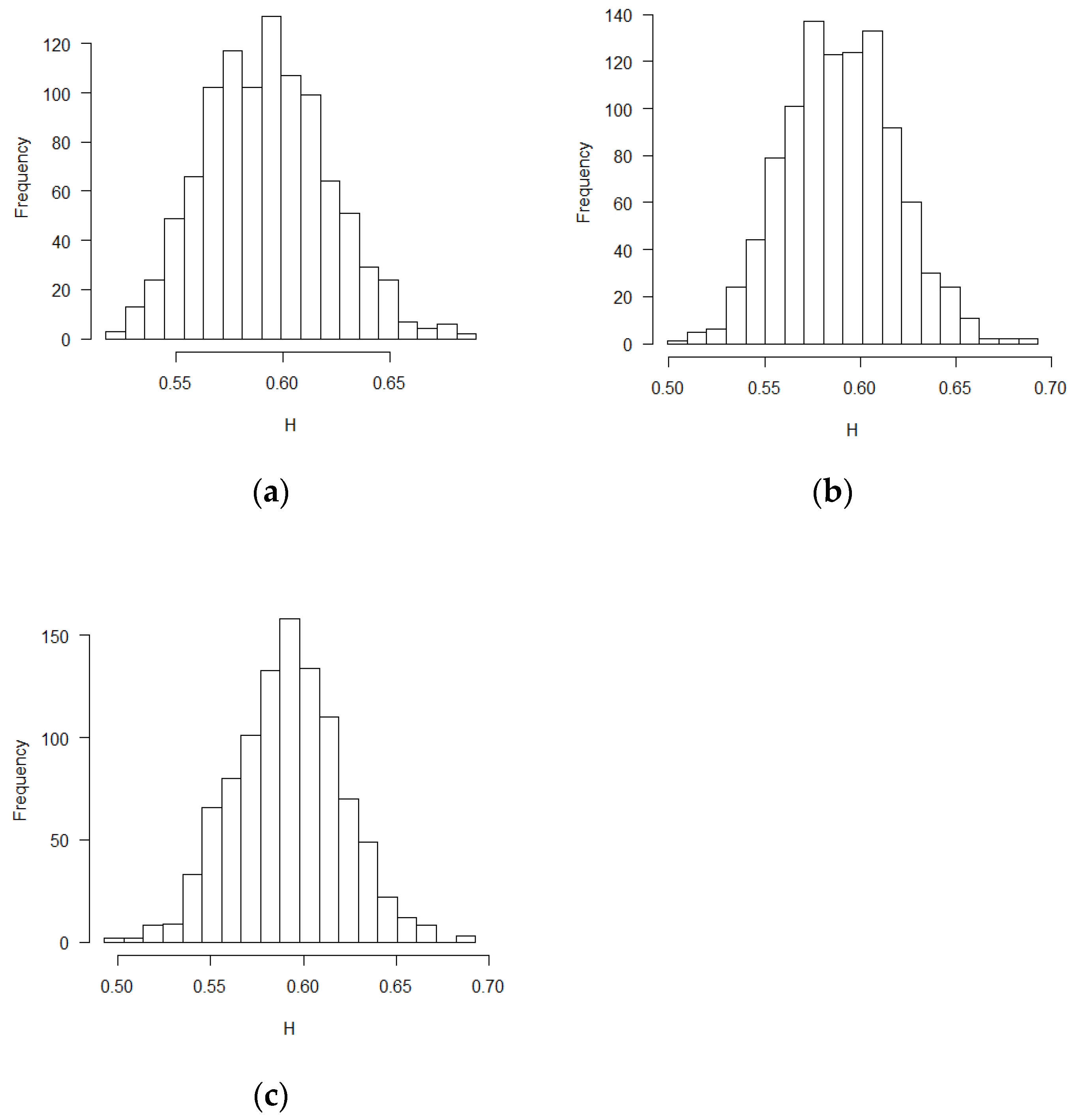
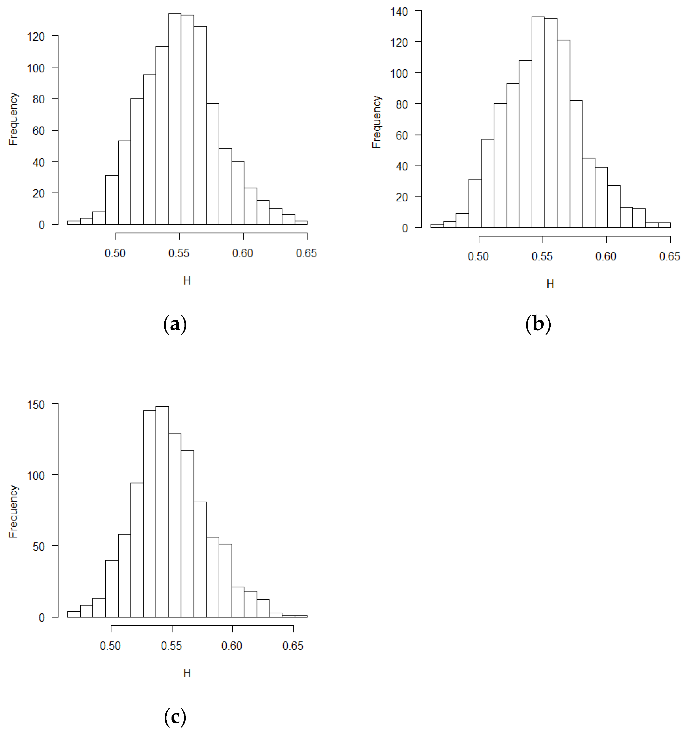
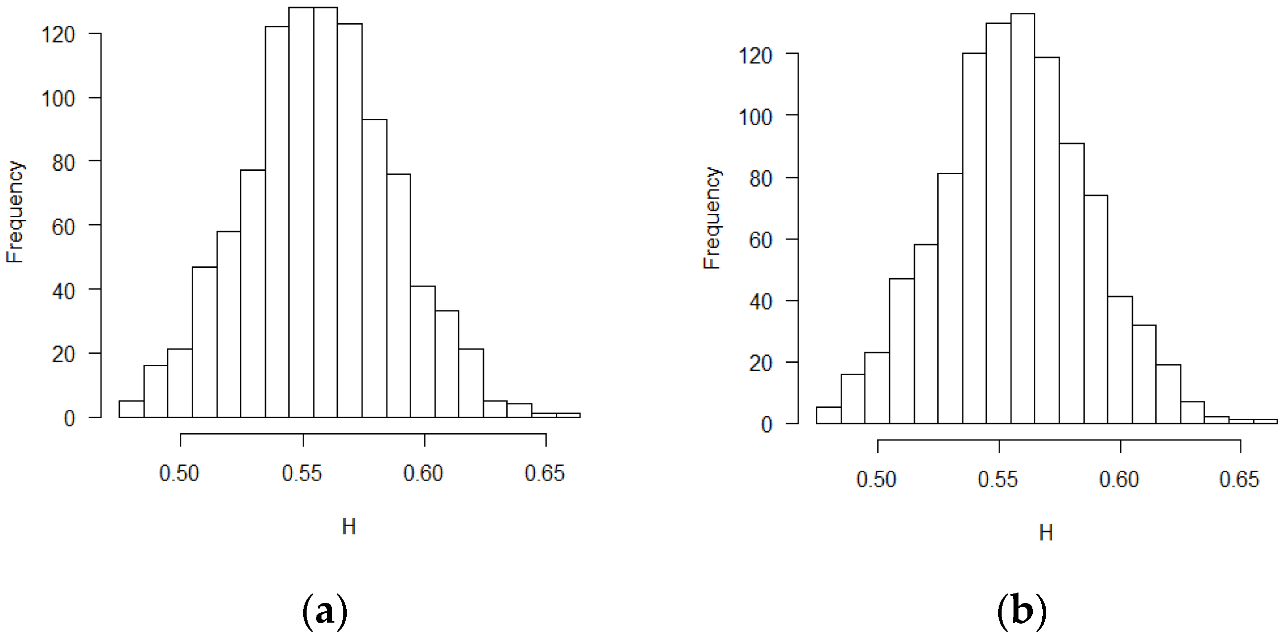
The mean and standard deviation of Hurst exponent estimations were tabulated in

Table 1. Hurst exponent estimations for covariate adaptive randomized clinical trials, ε’s ~increments of FBM, ${\mu }_1, {\mu }_2, {\beta }_1,{\beta }_2, p_1,p_2$ (0.5, 0.5, 1, 1, 0.5, 0.5).

		MLE Estimation			Peltler Lévy Véhel Hn,1 (1)
Designs		Mean	SD	p Value	Mean	SD	p Value
BR	No covariate	0.5921	0.0287	<0.0001	0.6056	0.0360	<0.0001
	Two discrete	0.5898	0.0288	<0.0001	0.6077	0.0347	<0.0001
	Two continuous	0.5915	0.0292	<0.0001	0.6067	0.0358	<0.0001
PS	No covariate	0.5504	0.0299	<0.0001	0.5608	0.0347	<0.0001
	Two discrete	0.5503	0.0299	<0.0001	0.5607	0.0348	<0.0001
	two continuous	0.5490	0.0300	<0.0001	0.5604	0.0351	<0.0001
SPB	No covariate	0.5568	0.0302	<0.0001	0.5685	0.0361	<0.0001
	Two discrete	0.5567	0.0302	<0.0001	0.5694	0.0354	<0.0001
	Two continuous	0.5576	0.0286	<0.0001	0.5691	0.0340	<0.0001

, in which another Hurst estimation method proposed by Peltler Lévy Véhel was used to validate the MLE results [30]. Two Hurst estimation methods reached similar results. The distribution of the estimates of H is close to normal distribution. The visual histograms are shown in Figure 1, Figure 2 and Figure 3. Mean estimated H values from the misspecification scenarios in Table 1 and Figure 1, Figure 2 and Figure 3 deviated from 0.5. All test of statistical significance test proved this conclusion with p value less than 0.0001 by t-test (Student’s t-Test) function in R software. According to the theoretical derivation results and simulation results, sequential test statistics do not follow a Brownian motion in the covariate adaptive randomized clinical trials sequential monitoring processes when error terms are correlated. Models with different covariate types reached similar conclusions.

4. Conditional Power for Covariate Adaptive Randomized Clinical Trials with Correlated Error Structures

Test statistics derived from covariate adaptive randomized clinical trials do not follow a Brownian motion in the sequential monitoring processes when ignoring the error term covariance patterns in the statistics test formula [15]. The independent increment property is not satisfied under the misspecification assumption for the covariate adaptive randomized clinical trials. Therefore, a more general form of stochastic process, fractional Brownian motion, was proposed for the misspecification scenarios. In this section, conditional powers were calculated and compared between the BM and the FBM methods.

Conditional power is the probability of rejecting the null hypothesis, given the interim data results up to the time of interim analysis [31]. Conditional power is used for the decisions regarding possible early termination, or proceeding to the original plan, or increasing the sample sizes in the clinical trial interim analyses. The evaluation of the conditional power can predict the long-term clinical trial study results based on the partially observed data.

Under the null hypothesis of no treatment effect for the clinical trial, $Z_t$ is the sequential test statistic at time t. Normalized $Z_t$ from the estimated of β$\left(t\right)$ in the covariate adaptive randomized clinical trial can be transformed to the B value as $B_H\left(t\right)$ = $Z_t{t}^{1/2}$. Assuming time $t>s$, the conditional probability can be calculated with Brownian motion: $CP=P\left(Z_t\ge a|Z_s=b\right)=1-\Phi (\frac{a{t}^{1/2}-b{s}^{1/2}}{\sqrt{t-s}}$) [10,32]. When the treatment effect is not equal in two groups, Brownian motion would have a drift parameter $\theta$. Brownian motion with drift follows the normal distribution with mean $\theta \left(t-s\right)$ and variance $(t-s$). The conditional power with drift is expressed as: $CP=1-\Phi (\frac{a{t}^{1/2}-b{s}^{1/2}-\theta \left(t-s\right)}{\sqrt{t-s}}$) [10,33].

The conditional probability under null hypothesis in terms of FBM was proposed in Lai et al. [34] expressed as:

$$CP=P\left(B_H\left(t_N\right)\ge s_N|B_H\left(t_n\right)=s_n\dots B_H\left(t_2\right)=s_2, B_H\left(t_1\right)=s_1\right)=1-\Phi \left(\frac{s_N-{\mu }_{H_n}}{{\sigma }_{H_n}}\right)$$

(7)

The conditional distribution in the Equation (7) is normally distributed as $N({\mu }_{H_n}$, ${\sigma }_{H_n}^2$). $\sum$ is the variance- covariance matrix of $B_H\left(t_N\right)$ and $B_H\left(t_n\right)\dots B_H\left(t_2\right), B_H\left(t_1\right)$, denoted as [$\begin{array}{cc}{\sum }_{11}& {\sum }_{12}\\ {\sum }_{21}& {\sum }_{22}\end{array}$]. $\sum$ is a symmetric matrix. ${\mu }_{H_n}={\sum }_{12}{\sum }_{22}^{-1}{\mu }_n$. ${\sigma }_{H_n}^2={\sum }_{11}-{\sum }_{12}{\sum }_{22}^{-1}{\sum }_{21}$. ${\mu }_n$ = ($B_H\left(t_n\right)\dots B_H\left(t_2\right), B_H\left(t_1\right){)}^t$ [34].

A two-stage simulation strategy was used to calculate the conditional power [35]. Recruited time $t$ was divided into two parts by the time point $ti.fix$, which resembled the interim analysis time point in the real clinical trial. The first part before the time point $ti.fix$, which is called the fixed part, includes the already known data information. The second part after the time point $ti.fix$ and until $t=1$ is called the unknown part. The empirical result was denoted as the analyzed data from $ti.fix$ to $t=1$ by 1000 simulations. It was assumed that the empirical results can respond the consequence at the end of the whole clinical trial.

Based on the Formula (7), CPs with the assumptions of the BM and FBM were calculated respectively for the fixed part, from $t=0$ to $t=ti.fix$. In Formula (7), $s_1$, $s_2$,..., $s_n$ are the observed values before $t_N$. The mean ${\mu }_{H_n}$ and ${\sigma }_{H_n}$ are described in the definition of Equation (7). The conditional power was denoted as CP (BM) under BM assumption with $H=0.5$. If the conditional power was calculated under the FBM assumption with the estimated H value by MLE approach, this was denoted as CP (FBM).

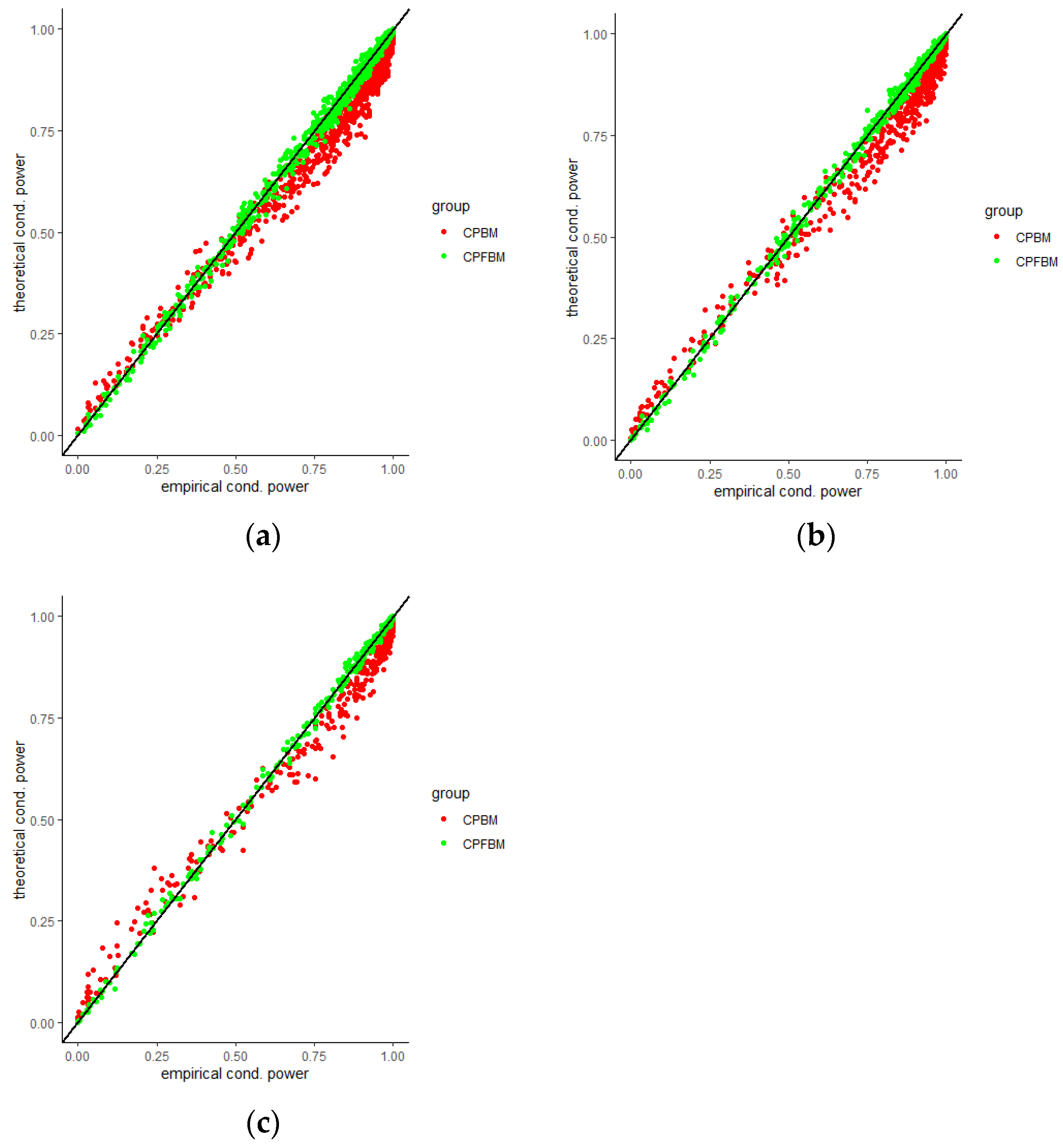
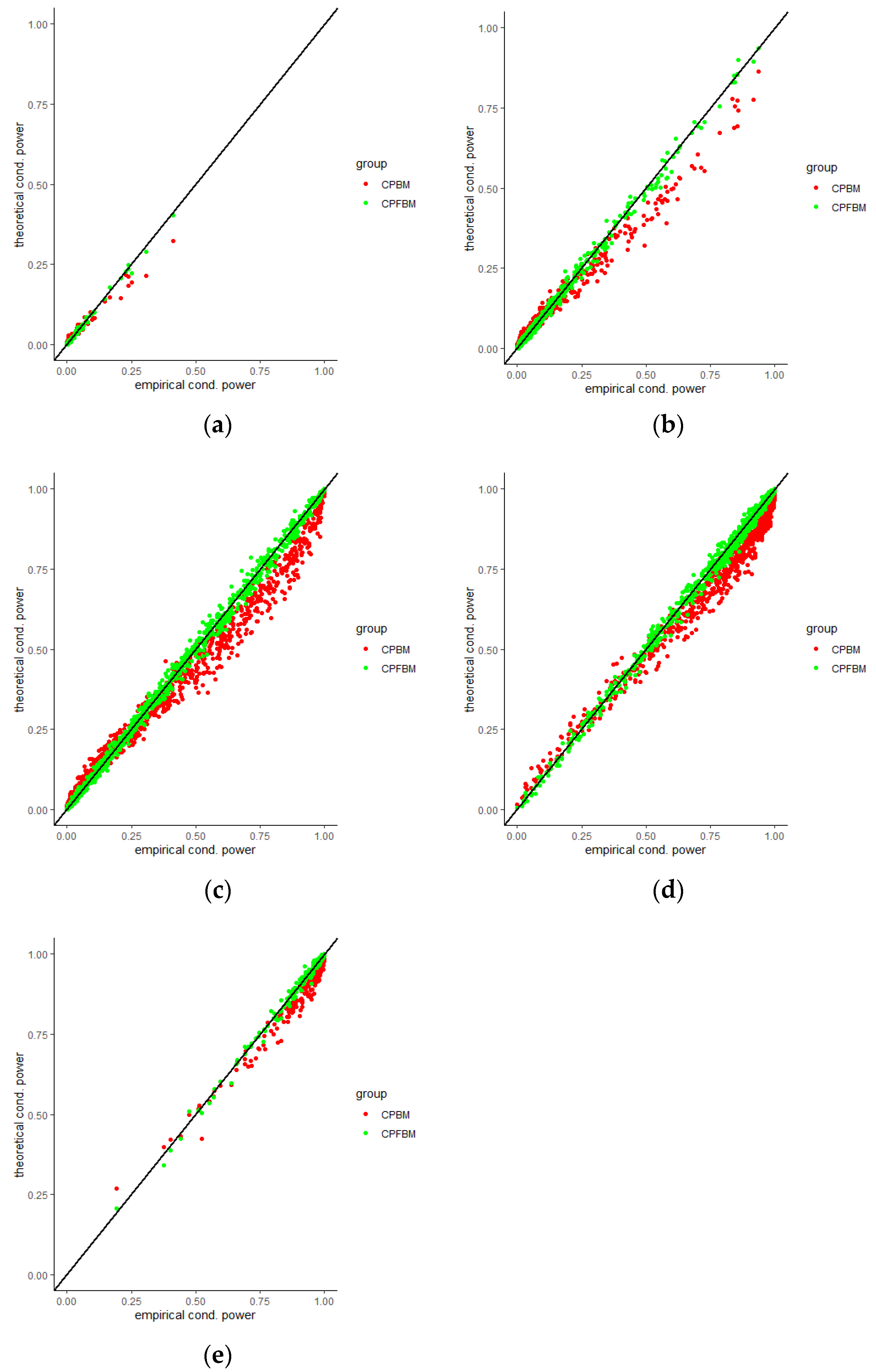
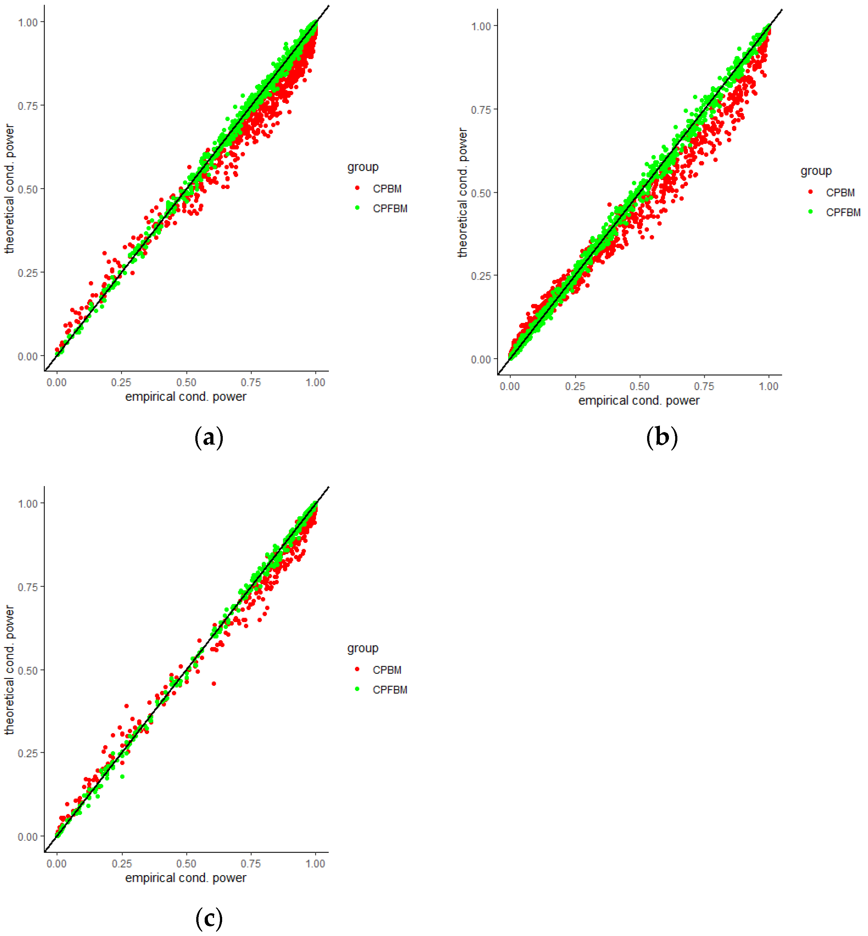
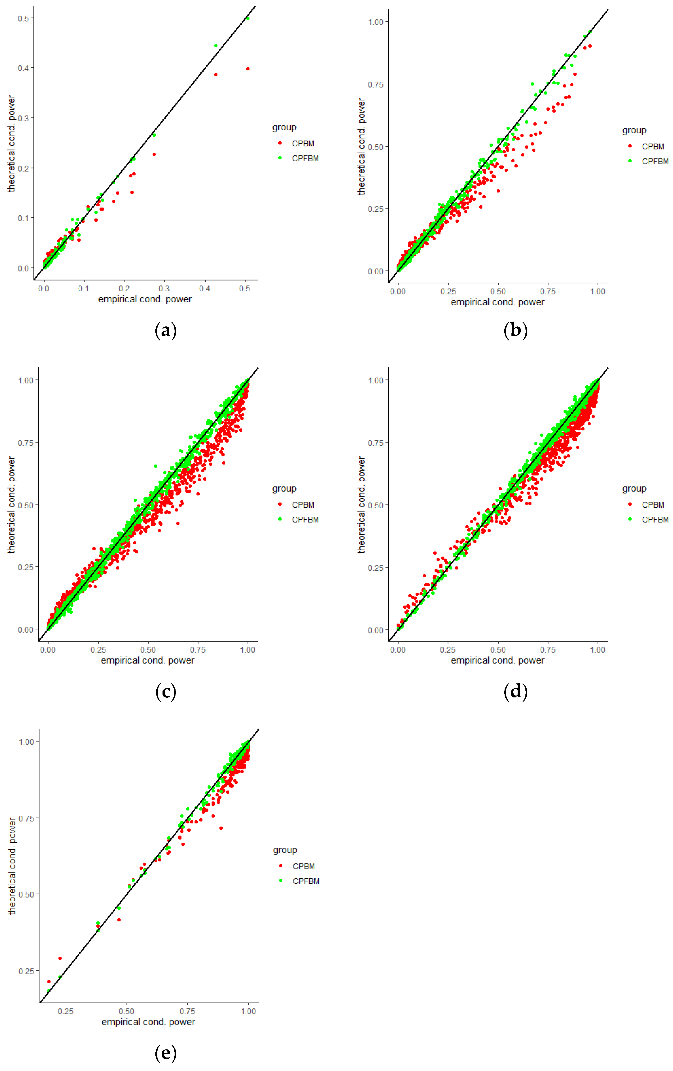
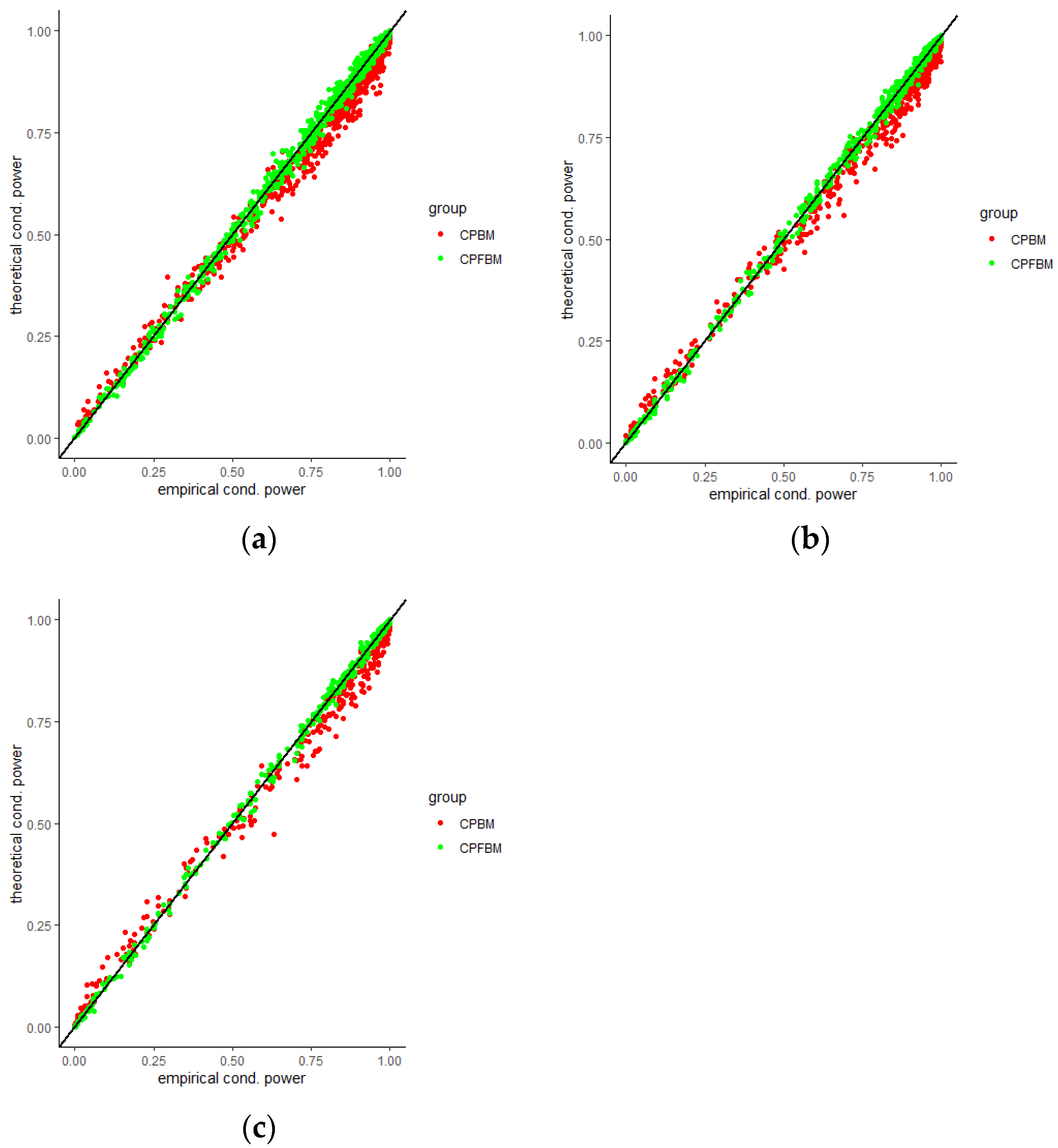
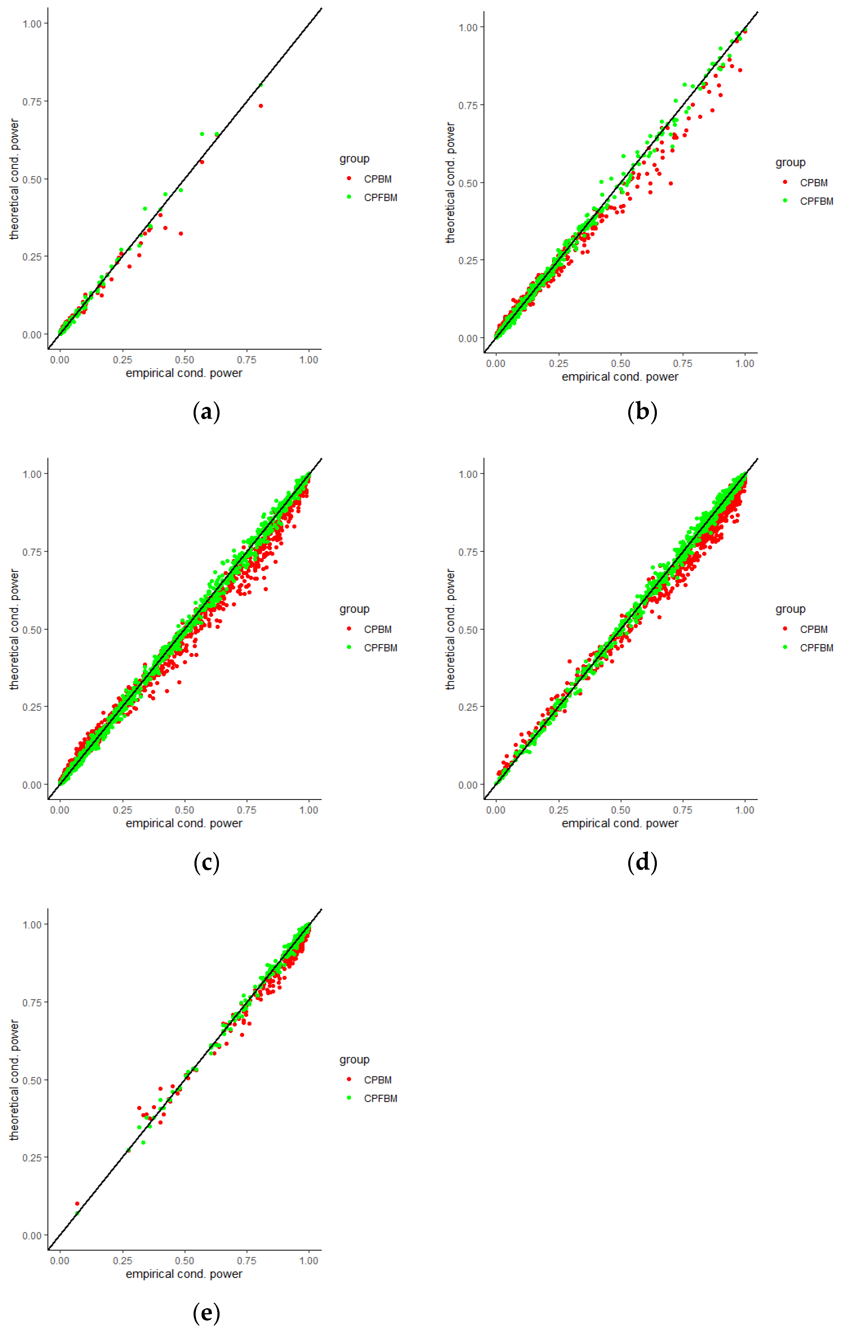
CP (empirical) was assumed to predict the results at the end of the whole clinical trial ($t=1$) with the formula CP (empirical)$=$ Count ($Z\left(t_N\right)>1.96)/1000$. 1.96 is the critical value for the hypothesis test with alpha $=0.05$ at $t=1$. CP (empirical), among 1000 replications, was treated as the standard criterion to compare with theoretical values CP (BM) and CP (FBM) [35]. Scatter plots for CP (BM), CP (FBM) and empirical CPs virtually demonstrated the consistency between the theoretical and empirical data.

Scenarios were simulated when a Brownian motion showed a mean shift upwards with drift. Assume that B$\left(t\right)$ is a standard Brownian motion process. A new Brownian motion process $U\left(t\right)$ with drift would be shown as $U\left(t\right)=\theta t+{\sigma }^{2}B\left(t\right), t\ge 0$. $\theta$ is the drift parameter. Assuming ${\sigma }^2=1$, different parameters ($\theta =0, 0.5, 1, 1.5, 2)$ were illustrated in the conditional power simulation processes. ${\mu }_{H_n}$ in the equation (7) corresponded with the drift parameters in the simulations. In addition, different interim time points, $ti.fix=0.7, 0.8, 0.9,$ were evaluated respectively.

In this section, a total sample size of 4000 participants was illustrated with 40 interim time points, although the actual number of interim analyses is much fewer. The error terms of the model were not independent and identically distributed but were assumed to follow increments of fractional Brownian motion with the Hurst exponent $H=0.9$. In this study, $B_H\left(t\right)$ were calculated first from sequential monitoring test statistics (3) under misspecification scenarios. H values were calculated based on the $B_H\left(t\right).$ Then, conditional powers were performed using Equation (7) with $B_H\left(t\right)$ from sequential processes.

We evaluated the performances of CP (BM) and CP (FBM), compared with CP (empirical) under different drift parameters and $ti.fix$ time points in

Table 2. CPs under misspecification scenarios: ε’s~increments of FBM, H = 0.9, drift = 0.

${\mathit{\mu }}_1, {\mathit{\mu }}_2, {\mathit{\beta }}_1,{\mathit{\beta }}_2, {\mathit{p}}_1,{\mathit{p}}_2$	ti.fix = 0.7	Designs	CP (Empirical)	CP (BM)	CP (FBM)	H
(0.5, 0.5)	No covariate	BR	0.0059	0.0062	0.0059	0.5890
		PS	0.0094	0.0093	0.0093	0.5494
		SPB	0.0093	0.0095	0.0093	0.5569
(0.5, 0.5, 1, 1, 0.5, 0.5)	Two discrete	BR	0.0043	0.0049	0.0041	0.5875
		PS	0.0094	0.0093	0.0093	0.5494
		SPB	0.0123	0.0120	0.0123	0.5550
(0.5, 0.5, 1, 1)	Two continuous	BR	0.0050	0.0053	0.0050	0.5883
		PS	0.0139	0.0137	0.0141	0.5477
		SPB	0.0079	0.0081	0.0078	0.5583

,

Table 3. CPs under misspecification scenarios: ε’s~increments of FBM, H = 0.9, drift = 0.5.

${\mathit{\mu }}_1, {\mathit{\mu }}_2, {\mathit{\beta }}_1,{\mathit{\beta }}_2, {\mathit{p}}_1,{\mathit{p}}_2$	ti.fix = 0.7	Designs	CP (Empirical)	CP (BM)	CP (FBM)	H
(0.5, 0.5)	No covariate	BR	0.0816	0.0776	0.0817	0.5889
		PS	0.0931	0.0903	0.0926	0.5494
		SPB	0.0940	0.0903	0.0935	0.5568
(0.5, 0.5, 1, 1, 0.5, 0.5)	Two discrete	BR	0.0824	0.0774	0.0812	0.5874
		PS	0.0931	0.0903	0.0926	0.5493
		SPB	0.1020	0.0987	0.1019	0.5549
(0.5, 0.5, 1, 1)	Two continuous	BR	0.0760	0.0728	0.0758	0.5882
		PS	0.1013	0.0982	0.1010	0.5476
		SPB	0.0911	0.0879	0.0905	0.5582

,

Table 4. CPs under misspecification scenarios: ε’s~increments of FBM, H = 0.9, drift = 1.

${\mathit{\mu }}_1, {\mathit{\mu }}_2, {\mathit{\beta }}_1,{\mathit{\beta }}_2, {\mathit{p}}_1,{\mathit{p}}_2$	ti.fix = 0.7	Designs	CP (Empirical)	CP (BM)	CP (FBM)	H
(0.5, 0.5)	No covariate	BR	0.3896	0.3647	0.3893	0.5887
		PS	0.3861	0.3720	0.3852	0.5491
		SPB	0.3868	0.3704	0.3864	0.5566
(0.5, 0.5, 1, 1, 0.5, 0.5)	Two discrete	BR	0.3927	0.3666	0.3920	0.5872
		PS	0.3861	0.3720	0.3851	0.5490
		SPB	0.4011	0.3854	0.3996	0.5547
(0.5, 0.5, 1, 1)	Two continuous	BR	0.3911	0.3630	0.3898	0.5880
		PS	0.3831	0.3712	0.3820	0.5474
		SPB	0.3854	0.3700	0.3855	0.5580

,

Table 5. CPs under misspecification scenarios: ε’s~increments of FBM, H = 0.9, drift = 2.

${\mathit{\mu }}_1, {\mathit{\mu }}_2, {\mathit{\beta }}_1,{\mathit{\beta }}_2, {\mathit{p}}_1,{\mathit{p}}_2$	ti.fix = 0.7	Designs	CP (Empirical)	CP (BM)	CP (FBM)	H
(0.5, 0.5)	No covariate	BR	0.9788	0.9685	0.9784	0.5878
		PS	0.9587	0.9528	0.9586	0.5482
		SPB	0.9618	0.9551	0.9619	0.5557
(0.5, 0.5, 1, 1, 0.5, 0.5)	Two discrete	BR	0.9779	0.9670	0.9774	0.5863
		PS	0.9587	0.9528	0.9586	0.5481
		SPB	0.9634	0.9565	0.9629	0.5537
(0.5, 0.5, 1, 1)	Two continuous	BR	0.9771	0.9670	0.9767	0.5870
		PS	0.9570	0.9505	0.9567	0.5465
		SPB	0.9667	0.9594	0.9665	0.5571

,

Table 6. CPs under misspecification scenarios: ε’s~increments of FBM, H = 0.9, drift = 1.5, ti.fix = 0.7.

${\mathit{\mu }}_1, {\mathit{\mu }}_2, {\mathit{\beta }}_1,{\mathit{\beta }}_2, {\mathit{p}}_1,{\mathit{p}}_2$	ti.fix = 0.7	Designs	CP (Empirical)	CP (BM)	CP (FBM)	H
(0.5, 0.5)	No covariate	BR	0.8100	0.7744	0.8081	0.5883
		PS	0.7675	0.7507	0.7669	0.5487
		SPB	0.7732	0.7533	0.7727	0.5562
(0.5, 0.5, 1, 1, 0.5, 0.5)	Two discrete	BR	0.8010	0.7686	0.7997	0.5868
		PS	0.7675	0.7507	0.7669	0.5487
		SPB	0.7809	0.7616	0.7800	0.5543
(0.5, 0.5, 1, 1)	Two continuous	BR	0.8111	0.7747	0.8089	0.5876
		PS	0.7619	0.7451	0.7607	0.5470
		SPB	0.7766	0.7569	0.7760	0.5576

,

Table 7. CPs under misspecification scenarios: ε’s~increments of FBM, H = 0.9, drift = 1.5, ti.fix = 0.8.

${\mathit{\mu }}_1, {\mathit{\mu }}_2, {\mathit{\beta }}_1,{\mathit{\beta }}_2, {\mathit{p}}_1,{\mathit{p}}_2$	ti.fix = 0.8	Designs	CP (Empirical)	CP (BM)	CP (FBM)	H
(0.5, 0.5)	No covariate	BR	0.8705	0.8447	0.8697	0.5896
		PS	0.8234	0.8120	0.8231	0.5491
		SPB	0.8360	0.8214	0.8356	0.5568
(0.5, 0.5, 1, 1, 0.5, 0.5)	Two discrete	BR	0.8571	0.8348	0.8568	0.5877
		PS	0.8234	0.8120	0.8231	0.5490
		SPB	0.8401	0.8260	0.8402	0.5558
(0.5, 0.5, 1, 1)	Two continuous	BR	0.8701	0.8445	0.8695	0.5889
		PS	0.8186	0.8071	0.8178	0.5476
		SPB	0.8374	0.8224	0.8372	0.5577

and

Table 8. CPs under misspecification scenarios: ε’s~increments of FBM, H = 0.9, drift = 1.5, ti.fix = 0.9.

${\mathit{\mu }}_1, {\mathit{\mu }}_2, {\mathit{\beta }}_1,{\mathit{\beta }}_2, {\mathit{p}}_1,{\mathit{p}}_2$	ti.fix = 0.9	Designs	CP (Empirical)	CP (BM)	CP (FBM)	H
(0.5, 0.5)	No covariate	BR	0.9041	0.8933	0.9041	0.5910
		PS	0.8732	0.8658	0.8725	0.5496
		SPB	0.8826	0.8746	0.8822	0.5576
(0.5, 0.5, 1, 1, 0.5, 0.5)	Two discrete	BR	0.9052	0.8931	0.9049	0.5888
		PS	0.8732	0.8658	0.8725	0.5495
		SPB	0.8857	0.8781	0.8856	0.5563
(0.5, 0.5, 1, 1)	Two continuous	BR	0.9107	0.9002	0.9108	0.5905
		PS	0.8670	0.8609	0.8669	0.5482
		SPB	0.8816	0.8739	0.8813	0.5574

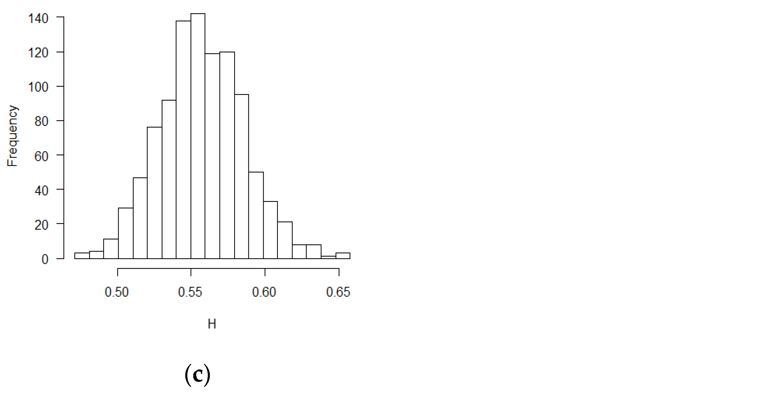
. Figure 4, Figure 5, Figure 6, Figure 7, Figure 8 and Figure 9 were the scatter plots with x axis representing the theoretical CPs and y axis representing the empirical CPs. Green dots in the figures are the CP (FBM), while red dots are the CP (BM). Based on the results from the Tables, the mean estimations of the Hurst coefficients deviated away from 0.5 under different scenarios. Assuming the treatment effects are equal between two groups with drift parameter $\theta =0$, CPs are small and close to 0. CPs increased dramatically along with the increase in drift parameter values. Different $ti.fix=0.7, 0.8, 0.9$ resume the interim analysis time points in the simulations. CPs increased as $ti.fix$ time values increased, since the interim analysis time point is closer to the end of the trial. When $H>0.5$, most of the CP (FBM) values were greater than CP (BM) values. From all Tables, the majority of CP (FBM) values matched the CP (empirical) values better than the CP (BM) values.

5. Conclusions and Discussions

In this study, we investigated the sequential monitoring properties in covariate adaptive randomized clinical trials under the misspecification scenarios. We also performed numerical simulations under various situations in which the mean estimates of Hurst coefficient by MLE from the sequential test statistics under misspecification scenarios deviated from 0.5. Brownian motion is satisfied only when $H=0.5$. Therefore, the independent increment assumption was violated and Brownian motion was not appropriate for the sequential process. However, clinical researchers may not know the existence of the covariance in the error terms, and hence use the original classical statistic test under the misspecification scenarios, leading to non-Brownian motion trajectory of the test statistics under sequential analysis. Therefore, it is necessary to estimate the Hurst coefficient.

We calculated conditional powers for covariate adaptive randomized clinical trials with mis-specified error structures of the model under different covariate types, adaptive designs, drift parameters, and interim time points. Conditional powers based on the fractional Brownian motion (CP (FBM)) assumption resulted in better consistency with the standard empirical value (CP (empirical)) than conditional powers under the classical Brownian motion (CP (BM)) assumption. When the $H_{MLE}>0.5$, most conditional powers under the FBM assumption were greater than the conditional powers under the classical Brownian motion assumption. The fractional Brownian motion, incorporating a dependent increment assumption, would be a reasonable approach for the clinical trial sequential analyses. Even if the sequential procedure actually follows the Brownian motion, the application of the fractional Brownian motion technique would still be useful, since BM is a special case of FBM with $H=0.5$.