Kinetic Model for Drying in Frame of Generalized Fractional Derivatives

Abstract

In this article, the Lewis model was considered for the soybean drying process by new fractional differential operators to analyze the estimated time in $50{}^{\circ }\mathrm{C}$, $60{}^{\circ }\mathrm{C}$, $70{}^{\circ }\mathrm{C}$, and $80{}^{\circ }\mathrm{C}$. Moreover, we used dimension parameters for the physical meaning of these fractional models within generalized and Caputo fractional derivatives. Results obtained with generalized fractional derivatives were analyzed comparatively with the Caputo fractional, integer order derivatives and Page model for the soybean drying process. All results for fractional derivatives are discussed and compared in detail.

1. Introduction

Drying kinetic phenomena is an important tool for long-continued food storing conditions. It is based on the loss of humidity inside the foods. Moisture content has a direct impact on the reproduction of fungus, must, microbial, etc. These negative effects of humidity make the storage time of foods shorten and for this reason, it raises the cost burden.

Mathematical modeling formulas are an effective and useful instrument for predicting some real world problems, such as the growth of microorganisms, the spread of outbreak diseases, tumor cell growth, and drying kinetic models. If we mention the effectiveness of the current ordinary differential models, we can clearly say that fractional differential equations are more alternative and efficient tools than integer order counterparts.

Diffusion process models heat and mass transfer in solid matters. This process can be applied with some differences on the drying kinetics of foods. Agutter et al. [1] described this diffusion process in living organisms with the movements of particles inside the cells.

Fractional calculus has been rising in popularity in the last decades. Especially, fractional differential modeling problems give more accurate results due to having a non-locality and memory effect. However, the dimension of quantities has great importance for the physical meaning of the problems. A new parameter must be used for preserving the dimension of quantities on fractionalizing modeling problems [2,3]. Fractional derivatives are alternative tools to try to explain better anomalous diffusion process with real data. For this reason, Simpson et al. [4] studied fractional mass transfer modeling in food drying, also Ramírez et al. [5] analyzed the drying analysis of apple slices in view of fractional calculus.

Modeling of mass transfer can be obtained by Fick’s Law. The fractional version of Fick’s Law can be found in [6]. Although classical Lewis model describes exponential behavior of diffusion, fractional Lewis model describes the non-exponential behavior of diffusion and it is called an anomalous diffusion [7].

The grain drying process speed depends on the conditions such as temperature, airflow, and mechanical drying systems. Besides, drying kinetic models show the estimated time needed for the optimum loss of humidity. These models take into account temperature effect, moisture content, and airflow. Fick’s second law explains rates of diffusion involving both time and space

$$\frac{\partial Y}{\partial t}=D{\nabla }^{2}Y,$$

(1)

where D is the diffusion coefficient and Y is the moisture content of the food.

Lewis model [8] is based on thin layer drying with temperature effect

$$\frac{\partial Y}{\partial t}=-k(Y\left(t\right)-Y_e),$$

(2)

where $Y_e$ is equilibrium moisture content and k is a constant of drying has dimension min${}^{-1}$. If we solve Equation (2), then we have the following solution

$$Y\left(t\right)=(Y_0-Y_e)e^{-kt}+Y_e,$$

(3)

where $Y_0$ is the initial moisture content inside the food.

Page’s model [9] is the modified version of Lewis model with a changing parameter in the exponential function

$$Y\left(t\right)=(Y_0-Y_e)e^{-k{t}^n}+Y_e,$$

(4)

where n is an adjustment parameter used for fitting data. This method is more successful on fitting real data than the Lewis method.

Fractional calculus has seen a rising in popularity in recent decades. The most important reason for this is having applications in real world problems and its ability to obtain better results than ordinary counterparts. The first known fractional derivative definitions are Riemann–Liouville and Liouville–Caputo fractional derivatives. In recent years, new fractional derivative definitions have been introduced by Caputo–Fabrizio (CF) [10], Atangana–Baleanu (AB) [11], and generalized AB [12]. Several studies were published involving these new fractional derivative definitions [13,14,15,16,17,18,19,20,21,22]. We can mention countless studies in this area, therefore we want to give some of them: Sekerci et al. [23,24] Kumar et al. [25], Ullah et al. [26], Singh et al. [27], Jajarmi et al. [28], Yusuf et al. [29], Qureshi et al. [30,31], Bas et al. [32], and so on [33,34,35,36]. Generalized fractional integrals and derivatives are defined by Katugampola [37,38]. This new type of fractional derivative shows the characteristic of both Riemann–Liouville while $\rho \to 1$ and the Hadamard [39] while $\rho \to 0$. Its Caputo form is introduced in [40].

Recently, Matias et al. [41] have studied fractional counterpart of Lewis model (2) within Caputo fractional derivative and they have achieved fitting experimental data with Caputo fractional version of Lewis model (2). Nicolin et al. studied the empirical drying model with fractional order [42].

In this study, we handled the Lewis model (see Equation (2)) within generalized fractional derivatives, with a parameter for preserving the dimension on fractional equations. We considered the soybean drying conditions at $50{}^{\circ }\mathrm{C}$, $60{}^{\circ }\mathrm{C}$, $70{}^{\circ }\mathrm{C}$, and $80{}^{\circ }\mathrm{C}$. We analyzed these results with generalized fractional derivatives, including two parameters as $\alpha$ order and real $\rho$ value, comparatively with the Caputo fractional and integer order derivatives for Lewis model and Page model (4).

2. Mathematical Background

Definition 1.

[43] The Caputo fractional derivative is given as, $\alpha >0$, $\alpha \in \mathbb{R}$ ve $n-1\le \alpha <n$, $n\in \mathbb{N}$,

$$\begin{array}{c}\hfill {}_a^C{D}_x^{\alpha }f\left(t\right)=\frac{1}{\mathsf{\Gamma }\left(n-\alpha \right)}\underset{a}{\overset{x}{\int }}\frac{d^{n}f\left(t\right)}{d{t}^n}{\left(x-t\right)}^{n-\alpha -1}dt.\end{array}$$

Definition 2.

[37] The generalized left and right fractional integrals of complex order α, $Re\left(\alpha \right)>0$ and $\rho \in {\mathbb{R}}^{+}$ are given respectively by

$$\begin{array}{ccc}\hfill {}_a{I}^{\alpha ,\rho }f\left(t\right)& =& \frac{1}{\mathsf{\Gamma }\left(\alpha \right)}{\int }_a^t{\left(\frac{t^{\rho }}{\rho }-\frac{x^{\rho }}{\rho }\right)}^{\alpha -1}f\left(x\right)d_{\rho }x,\hfill \end{array}$$

(5)

and

$$\begin{array}{ccc}\hfill I_b^{\alpha ,\rho }f\left(t\right)& =& \frac{1}{\mathsf{\Gamma }\left(\alpha \right)}{\int }_t^b{\left(\frac{t^{\rho }}{\rho }-\frac{x^{\rho }}{\rho }\right)}^{\alpha -1}f\left(x\right)d_{\rho }x,\hfill \end{array}$$

(6)

where $d_{\rho }x=\frac{{\displaystyle dx}}{{\displaystyle x^{1-\rho }}}$

Definition 3.

[40] The generalized left and right fractional derivatives in the Caputo sense of complex order α, $Re\left(\alpha \right)>0$, and $\rho \in {\mathbb{R}}^{+}$ are given, respectively, by

$$\begin{array}{ccc}\hfill {}_a^C{D}^{\alpha ,\rho }f\left(t\right)& =& {}_a{I}^{n-\alpha ,\rho }{\gamma }^{n}f\left(t\right)\hfill \\ \hfill & =& \frac{1}{\mathsf{\Gamma }(n-\alpha )}{\int }_a^t{\left(\frac{t^{\rho }}{\rho }-\frac{x^{\rho }}{\rho }\right)}^{n-\alpha -1}{\gamma }^{n}f\left(x\right)d_{\rho }x,\hfill \end{array}$$

(7)

and

$$\begin{array}{ccc}\hfill {}^C{D}_b^{\alpha ,\rho }f\left(t\right)& =& I_b^{n-\alpha ,\rho }{\left(-\gamma \right)}^{n}f\left(t\right)\hfill \\ \hfill & =& \frac{1}{\mathsf{\Gamma }(n-\alpha )}{\int }_t^b{\left(\frac{t^{\rho }}{\rho }-\frac{x^{\rho }}{\rho }\right)}^{n-\alpha -1}{\left(-\gamma \right)}^{n}f\left(x\right)d_{\rho }x,\hfill \end{array}$$

(8)

where $\gamma =t^{1-\rho }\frac{d}{dt}$, $\rho >0$. If $\rho =1$ in this definition, we obtain a Caputo fractional derivative and if $\rho \to 0$, we obtain a Caputo–Hadamard fractional derivative defined in [40].

Theorem 1.

[44] $\rho —$Laplace transform of the function $f\left(t\right)$ is given as

$$L_{\rho }\left\{f\left(t\right)\right\}\left(s\right)={\int }_0^{\infty }{e}^{-s\frac{t^{\rho }}{\rho }}f\left(t\right)\frac{dt}{t^{1-\rho }},\rho >0,$$

(9)

where $f:[0,\infty )\to \mathbb{R}$ is a real valued function.

Theorem 2.

[44] $\rho —$Laplace transform of $\gamma f\left(t\right)$ is defined as follows,

$$L_{\rho }\left\{\gamma f\left(t\right)\right\}\left(s\right)=s{L}_{\rho }\left\{f\left(t\right)\right\}-f\left(0\right).$$

(10)

Theorem 3.

[44] Let $f\in A{C}_{\gamma }^n[0,a]$, $a>0$, $\alpha >0$, and ${\gamma }^k={\left(t^{1-\rho }\frac{d}{dt}\right)}^{k}f\left(t\right)$, $k=0,1,\dots ,n$ has exponential order $e^{c\frac{t^{\rho }}{\rho }}$, then we have

$$L_{\rho }{\{}_0^C{D}^{\alpha ,\rho }f\left(t\right)\}=s^{\alpha }\left[L_{\rho }\left\{f\left(t\right)\right\}-\sum _{k=0}^{n-1}{s}^{-k-1}\left({\gamma }^{k}f\right)\left(0\right)\right],$$

(11)

where $s>0$.

Lemma 1.

[44] $Re\left(\alpha \right)>0$ and $\left|\frac{a}{s^{\alpha }}\right|<1,$ the $\rho —$Laplace transform of some special functions are as below

i. 

$L_{\rho }\left\{E_{\alpha }\left(-a{\left(\frac{t^{\rho }}{\rho }\right)}^{\alpha }\right)\right\}=\frac{{\displaystyle s^{\alpha }}}{{\displaystyle s(s^{\alpha }+a)}}$.

ii. 

$L_{\rho }\left\{1-E_{\alpha }\left(-a{\left(\frac{t^{\rho }}{\rho }\right)}^{\alpha }\right)\right\}=\frac{{\displaystyle a}}{{\displaystyle s(s^{\alpha }+a)}}$.

iii. 

$L_{\rho }\left\{{\left(\frac{t^{\rho }}{\rho }\right)}^{\alpha -1}{E}_{\alpha ,\alpha }\left(-a{\left(\frac{t^{\rho }}{\rho }\right)}^{\alpha }\right)\right\}=\frac{{\displaystyle 1}}{{\displaystyle s^{\alpha }+a}}$.

iv. 

$L_{\rho }\left\{{\left(\frac{t^{\rho }}{\rho }\right)}^{\beta -1}{E}_{\alpha ,\beta }\left(a{\left(\frac{t^{\rho }}{\rho }\right)}^{\alpha }\right)\right\}=\frac{{\displaystyle s^{\alpha -\beta }}}{{\displaystyle s^{\alpha }-a}}$.

3. Main Results

In this section, we consider the Lewis model (see Equation (2)) within generalized and Caputo fractional derivatives by preserving dimension of the physical quantities for fractional operators. It has already been discussed in numerous studies that mathematical models based on fractional order derivatives give much better results than their integer order counterparts.

Caputo fractional derivative enables them to be used in physical, engineering, and biological problems due to having integer order initial conditions. Hence, we can mention clearly in the development of fractional calculus in real world problems began with the Caputo definition. In this context, drying kinetic modeling is considered by Caputo and generalized fractional derivative in the Caputo sense.

3.1. Lewis Drying Kinetic Model in Fractional Cases

We can give the model (Equation (2)) in fractional cases, generalized, and Caputo, so one can find analytical solutions by using Laplace transforms.

Starting from this, we can give the fractional version of the Lewis model (Equation (2)).

3.1.1. Drying Kinetic with Generalized Fractional Derivative

$${}_0^C{D}_t^{\alpha ,\rho }Y\left(t\right)=-k^{\alpha \rho }(Y\left(t\right)-Y_e),0<\alpha \le 1,$$

(12)

$$Y\left(0\right)=1,$$

(13)

If we take the $\rho$—Laplace transform of Equation (12) and using initial condition (Equation (13)), then we have

$$L_{\rho }\left\{{}_0^C{D}^{\alpha ,\rho }Y\left(t\right)\right\}\left(s\right)=L_{\rho }\left\{-k^{\alpha \rho }(Y\left(t\right)-Y_e)\right\}\left(s\right),$$

(14)

thus one can attain

$$\left(s^{\alpha }{L}_{\rho }\left\{Y\left(t\right)\right\}\left(s\right)-s^{\alpha -1}Y\left(0\right)\right)=L_{\rho }\{-k^{\alpha \rho }(Y\left(t\right)-Y_e)\}\left(s\right),$$

(15)

and from here, if we can take the inverse $\rho$–LT of the last equation, we can obtain analytical solution as follows

$$\begin{array}{c}\hfill Y\left(t\right)=Y\left(0\right)E_{\alpha }\left(-k^{\alpha \rho }{\left(\frac{t^{\rho }}{\rho }\right)}^{\alpha }\right)+Y_e\left[1-E_{\alpha }\left(-k^{\alpha \rho }{\left(\frac{t^{\rho }}{\rho }\right)}^{\alpha }\right)\right].\end{array}$$

(16)

3.1.2. Drying Kinetic with Caputo Fractional Derivative

$${}_0^C{D}_t^{\alpha }Y\left(t\right)=-k^{\alpha }(Y\left(t\right)-Y_e),0<\alpha \le 1,$$

(17)

$$Y\left(0\right)=1.$$

(18)

If we take the Laplace transform of Equation (17) and using initial condition (Equation (18)), then we have

$$L\left\{{}_0^C{D}^{\alpha }Y\left(t\right)\right\}\left(s\right)=-L\left\{-k^{\alpha }(Y\left(t\right)-Y_e)\right\}\left(s\right),$$

(19)

and from here, if we can take the inverse LT of the last equation, we can obtain analytical solution as follows

$$\begin{array}{c}\hfill Y\left(t\right)=(Y\left(0\right)-Y_e)E_{\alpha }\left(-k^{\alpha }{t}^{\alpha }\right)+Y_e.\end{array}$$

(20)

4. Comparative Results

In this section, we analyze drying kinetics for soybean in 50 ${}^{\circ }\mathrm{C},$ 60 ${}^{\circ }\mathrm{C},$ 70 ${}^{\circ }\mathrm{C},$ and 80 ${}^{\circ }\mathrm{C}$. Matias et al. [41] considered real data for the drying kinetics of soybean and managed to fit the data to the results obtained within Caputo fractional sense. From this point of view, we compared the generalized fractional derivative with Caputo, classical Lewis model, and Page model. We used all parameters, like $\alpha$ order and $k,Y_e,n$ constants from [41], during our study. We adapted the k parameter in the Caputo–Lewis model as $k^{\alpha }$ for preserving physical quantities and hence the value of k will change for each $\alpha$ parameters. We study to match generalized fractional results to the Caputo fractional results of [41].

Table 1. Parameter values of models [41].

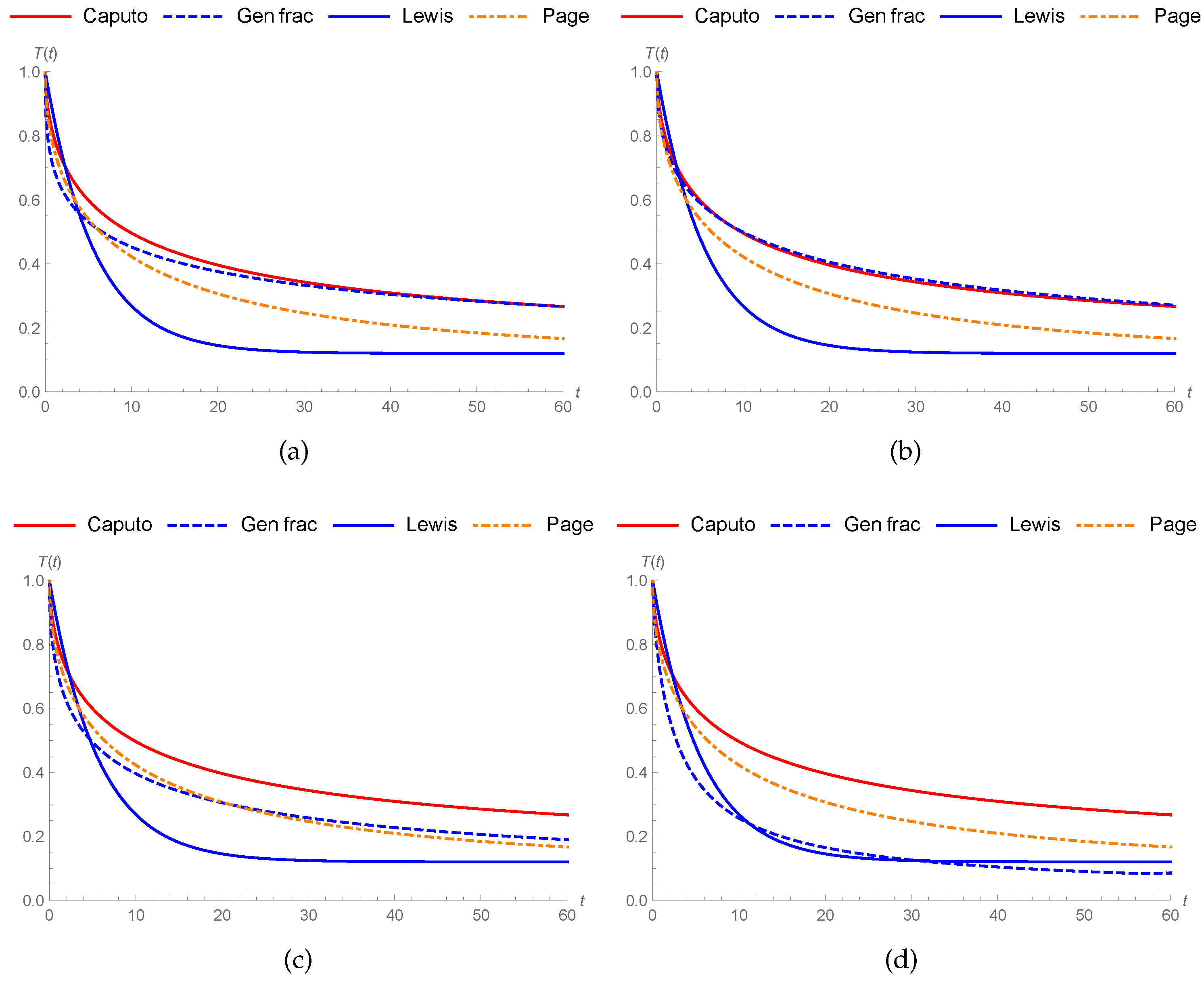
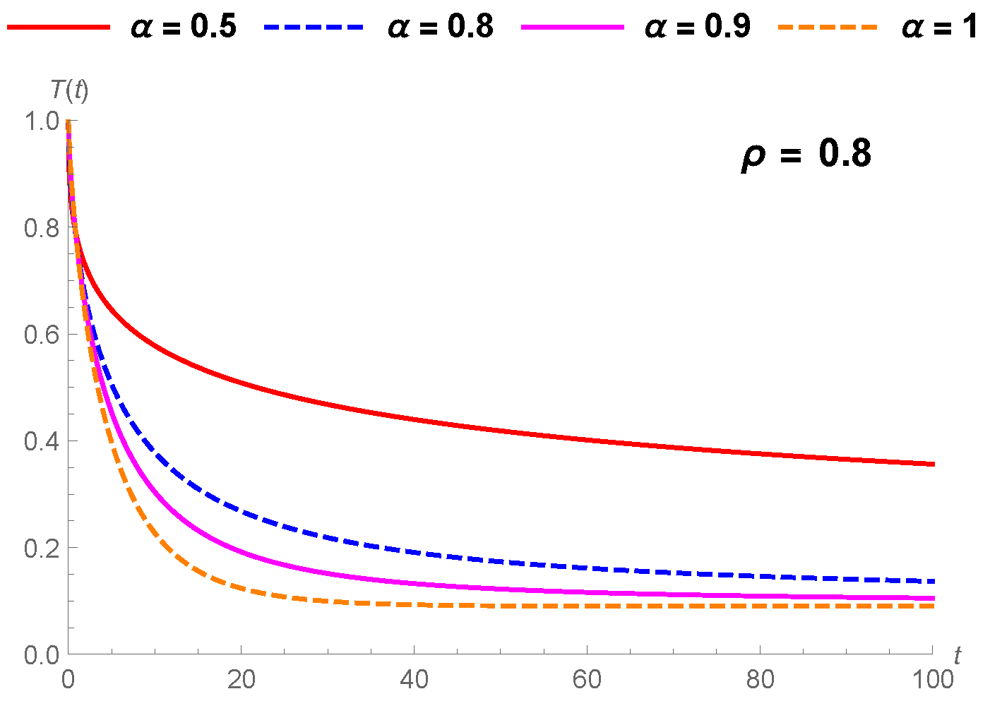
Figures	Parameters	Page	Lewis Classical	Lewis Caputo	Lewis Gen. Frac.
	k	0.31	0.178	0.0835014	0.0579262
Figure 1a	$Y_e$	0.10	0.12	0.09	0.01
	$\alpha$			0.57478	0.5
	$\rho$				0.8
	n	0.52
	k	0.31	0.178	0.0835014	0.0430676
Figure 1b	$Y_e$	0.10	0.12	0.09	0.01
	$\alpha$			0.57478	0.6
	$\rho$				0.8
	n	0.52
	k	0.31	0.178	0.0835014	0.0917365
Figure 1c	$Y_e$	0.10	0.12	0.09	0.01
	$\alpha$			0.57478	0.63
	$\rho$				0.8
	n	0.52
	k	0.31	0.178	0.0835014	0.187836
Figure 1d	$Y_e$	0.10	0.12	0.09	0.01
	$\alpha$			0.57478	0.9
	$\rho$				0.8
	n	0.52

,

Table 2. Parameter values of models [41].

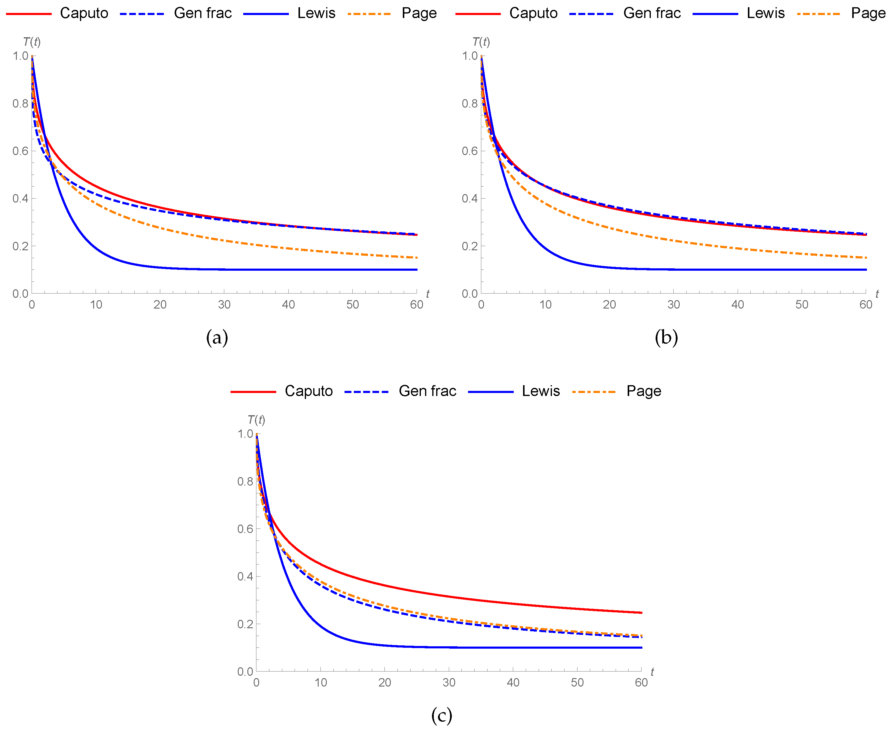
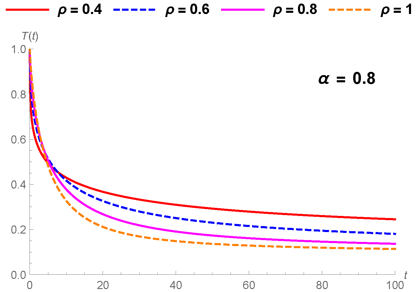
Figures	Parameters	Page	Lewis Classical	Lewis Caputo	Lewis Gen. Frac.
	k	0.39	0.23	0.109725	0.0911242
Figure 2a	$Y_e$	0.08	0.10	0.07	0.008
	$\alpha$			0.53	0.45
	$\rho$				0.85
	n	0.46
	k	0.39	0.23	0.109725	0.065617
Figure 2b	$Y_e$	0.08	0.10	0.07	0.001
	$\alpha$			0.53	0.52
	$\rho$				0.85
	n	0.46
	k	0.39	0.23	0.109725	0.142309
Figure 2c	$Y_e$	0.08	0.10	0.07	0.01
	$\alpha$			0.53	0.65
	$\rho$				0.95
	n	0.46

,

Table 3. Parameter values of models [41].

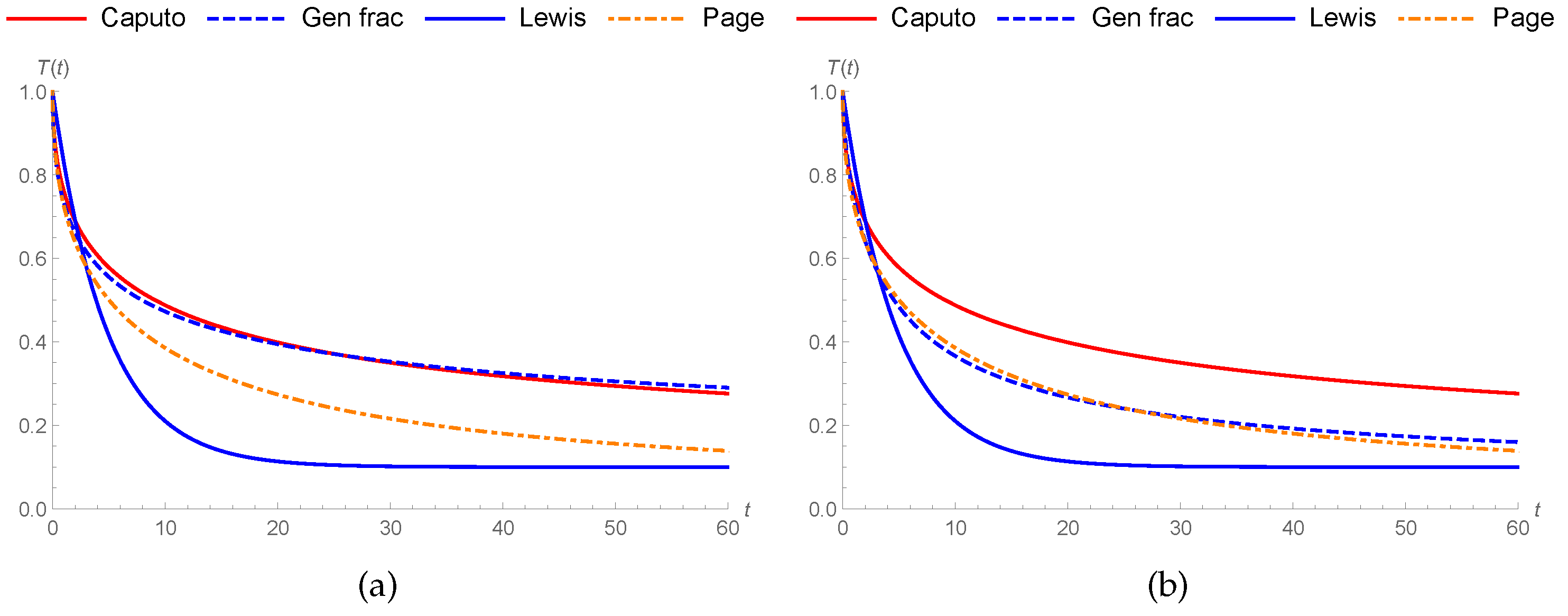
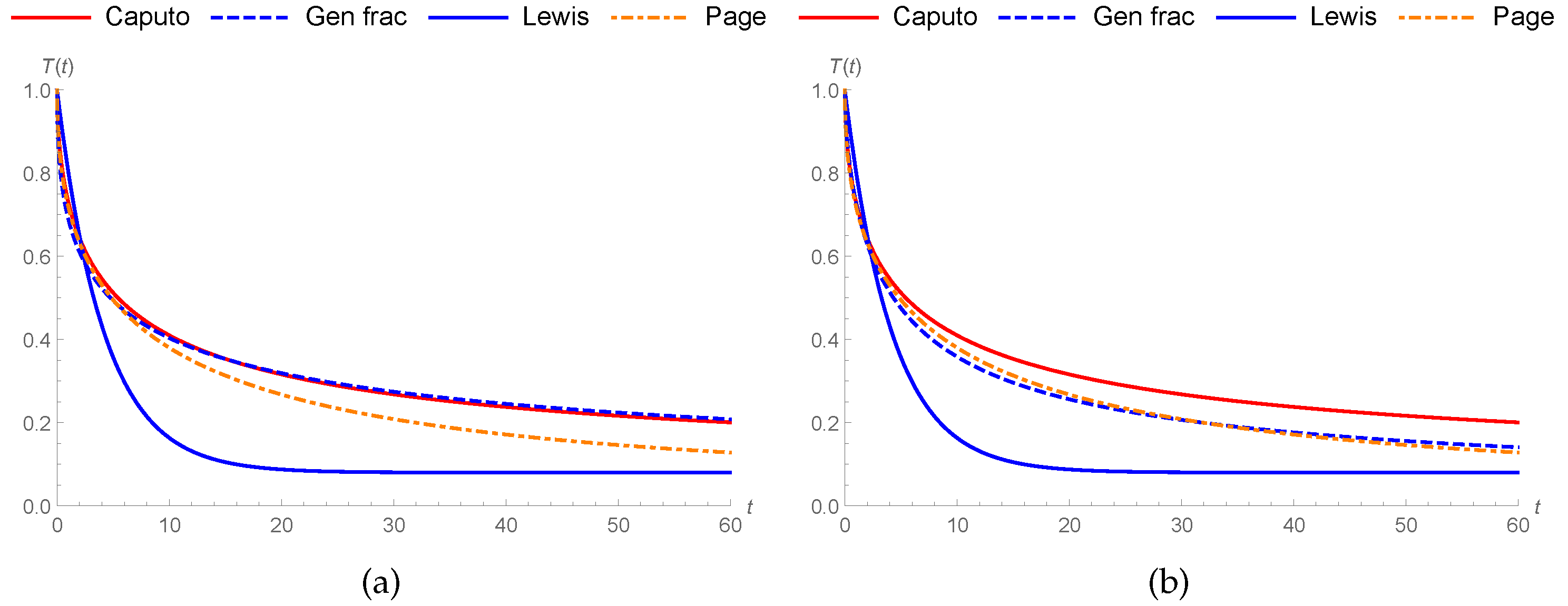
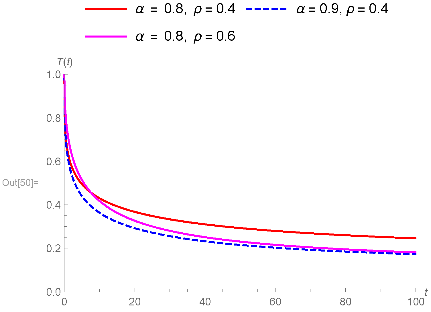
Figures	Parameters	Page	Lewis Classical	Lewis Caputo	Lewis Gen. Frac.
	k	0.35	0.21	0.0785997	0.0822175
Figure 3a	$Y_e$	0.07	0.10	0.05	0.1
	$\alpha$			0.50050	0.61
	$\rho$				0.79
	n	0.49
	k	0.35	0.21	0.0785997	0.126885
Figure 3b	$Y_e$	0.07	0.10	0.05	0.05
	$\alpha$			0.50050	0.85
	$\rho$				0.79
	n	0.49

and

Table 4. Parameter values of models [41].

Figures	Parameters	Page	Lewis Classical	Lewis Caputo	Lewis Gen. Frac.
	k	0.35	0.24	0.125972	0.106117
Figure 4a	$Y_e$	0.05	0.08	0.04	0.01
	$\alpha$			0.55	0.52
	$\rho$				0.9
	n	0.48
	k	0.35	0.24	0.125972	0.142309
Figure 4b	$Y_e$	0.05	0.08	0.04	0.01
	$\alpha$			0.55	0.65
	$\rho$				0.95
	n	0.48

show the parameters used in Figure 1, Figure 2, Figure 3 and Figure 4 respectively.

5. Discussion

In this section, we discuss drying kinetic models, which are Lewis (Equation (2)), Page (Equation (4)), and fractional Lewis Equations (Equation (12)) and (Equation (17)) involving generalized and Caputo fractional operators, respectively. We illustrate the governing drying kinetic equations with fractional, classical, and Page models. Matias et al. [41] considered real data for the soybean drying process and managed to fit the data to the results obtained within the Caputo fractional sense. From this point of view, we compared generalized fractional and classical derivatives to the Page model and made use of parameters, like $\alpha$ order of Caputo and $k,Y_e,n$ parameters, from [41] during our study.

We tried to match the generalized fractional results to the fractional result of [41]. Thus, we can easily say that the generalized fractional results are much better than the Caputo fractional results in all conditions in Figure 1a,b, Figure 2a,b, Figure 3a and Figure 4a. Furthermore, generalized fractional results work compatible with the Page model results in Figure 1c, Figure 2c, Figure 3b and Figure 4b. Also, we observed generalized fractional result approaches to classical Lewis model in Figure 1d. Figure 5, Figure 6 and Figure 7 compares the Lewis generalized fractional results under different $\alpha$ orders and real $\rho$ values. We show the effect of generalized fractional derivative on Lewis model under different finite times t = 5, 10, 20, 50, 100, and 200 for changing $\alpha ,\rho$ parameters in Figure 8, Figure 9 and Figure 10.

6. Conclusions

Consequently, we considered the Lewis model (Equation (2)), which was used for the grain drying process in view of generalized fractional and Caputo fractional derivatives. However, we used a parameter for preserving the dimension of fractional equations and hence, equations will have meaning from a physical viewpoint.

We analyzed the results based on scientific data for the soybean drying process and compared the results in view of Caputo and generalized fractional derivatives. We observed that the generalized fractional derivative gives compatible results with the Caputo fractional results in all conditions. It is worth noting that different real $\rho$ values differ when changing between Page and fractional results.

Eventually, generalized fractional derivatives give good results compatible with Caputo in all conditions for the Lewis model (Equation (2)), which was used for the grain drying process. The generalized fractional derivatives for the Lewis model gave more advantageous results than the integer order counterparts based on scientific data applied by Matias et al. [41].

References

- Agutter, P.S.; Malone, P.C.; Wheatley, D.N. Diffusion theory in biology: A relic of mechanistic materialism. J. Hist. Biol. 2000, 33, 71–111. [Google Scholar] [CrossRef] [PubMed]
- Garcia, J.R.; Calderon, M.G.; Ortiz, J.M.; Baleanu, D.; de Santiago, C.S.V. Motion of a particle in a resisting medium using fractional calculus approach. Proc. Rom. Acad. A 2013, 14, 42–47. [Google Scholar]
- Diethelm, K. A fractional calculus based model for the simulation of an outbreak of dengue fever. Nonlinear Dyn. 2013, 71, 613–619. [Google Scholar] [CrossRef]
- Simpson, R.; Jaques, A.; Nuńez, H.; Ramirez, C.; Almonacid, A. Fractional calculus as a mathematical tool to improve the modeling of mass transfer phenomena in food processing. Food Eng. Rev. 2013, 5, 45–55. [Google Scholar] [CrossRef]
- Ramírez, C.; Astorga, V.; Nuńez, H.; Jaques, A.; Simpson, R. Anomalous diffusion based on fractional calculus approach applied to drying analysis of apple slices: The effects of relative humidity and temperature. J. Food Process Eng. 2017, 40, e12549. [Google Scholar] [CrossRef]
- Metzler, R.; Klafter, J. The random walk’s guide to anomalous diffusion: A fractional dynamics approach. Phys. Rep. 2000, 339, 1–77. [Google Scholar] [CrossRef]
- Fomin, S.; Chugunov, V.; Hashida, T. Mathematical modeling of anomalous diffusion in porous media. Fract. Differ. Calc. 2011, 1, 1–28. [Google Scholar] [CrossRef]
- Lewis, W.K. The rate of drying of solid materials. Ind. Eng. Chem. 1921, 13, 427–432. [Google Scholar] [CrossRef]
- Page, G.E. Factors Influencing the Maximum Rates of Air Drying Shelled Corn in Thin Layers; Purdue University: West Lafayette, IN, USA, 1949. [Google Scholar]
- Caputo, M.; Fabrizio, M. A new definition of fractional derivative without singular kernel. Prog. Fract. Differ. Appl. 2015, 1, 1–13. [Google Scholar]
- Atangana, A.; Baleanu, D. New fractional derivatives with nonlocal and generalized kernel: Theory and application to heat transfer model. Therm. Sci. 2016, 20, 757–763. [Google Scholar] [CrossRef]
- Abdeljawad, T.; Baleanu, D. On fractional derivatives with generalized Mittag-Leffler kernels. Adv. Differ. Equ. 2018, 2018, 468. [Google Scholar] [CrossRef]
- Fernandez, A.; Özarslan, M.A.; Baleanu, D. On fractional calculus with general analytic kernels. Appl. Math. Comput. 2019, 354, 248–265. [Google Scholar] [CrossRef]
- Bas, E.; Ozarslan, R. Real world applications of fractional models by Atangana-Baleanu fractional derivative. Chaos Solitons Fractals 2018, 116, 121–125. [Google Scholar] [CrossRef]
- Bas, E.; Ozarslan, R.; Baleanu, D.; Ercan, A. Comparative simulations for solutions of fractional Sturm-Liouville problems with generalized operators. Adv. Differ. Equ. 2018, 2018, 350. [Google Scholar] [CrossRef]
- Abdeljawad, T. A Lyapunov type inequality for fractional operators with nonsingular Mittag-Leffler kernel. J. Inequal. Appl. 2017, 2017, 130. [Google Scholar] [CrossRef] [PubMed]
- Sekerci, Y.; Ozarslan, R. Respiration Effect on Plankton–Oxygen Dynamics in view of generalized time fractional derivatives. Phys. A Stat. Mech. Appl. 2019, 123942. [Google Scholar] [CrossRef]
- Sekerci, Y.; Ozarslan, R. Marine system dynamical response to a changing climate in frame of power law, exponential decay and Mittag-Leffler kernel. Math. Methods Appl. Sci. 2020, 43, 5480–5506. [Google Scholar] [CrossRef]
- Sekerci, Y.; Ozarslan, R. Oxygen-plankton model under the effect of global warming with nonsingular fractional order. Chaos Solitons Fractals 2020, 132, 109532. [Google Scholar] [CrossRef]
- Ozarslan, R.; Bas, E.; Baleanu, D.; Acay, B. Fractional physical problems including wind-influenced projectile motion with Mittag-Leffler kernel. AIMS Math. 2020, 5, 467. [Google Scholar] [CrossRef]
- Ozarslan, R. Microbial Survival and Growth Modeling in Frame of Nonsingular Fractional Derivatives. Math. Meth. Appl. Sci. 2020, 1–19. [Google Scholar] [CrossRef]
- Acay, B.; Ozarslan, R.; Bas, E. Fractional physical models based on falling body problem. AIMS Math. 2020, 5, 2608–2628. [Google Scholar] [CrossRef]
- Sekerci, Y.; Ozarslan, R. Dynamic analysis of time fractional order oxygen in a plankton system. Eur. Phys. J. Plus 2020, 135, 88. [Google Scholar] [CrossRef]
- Sekerci, Y. Climate change effects on fractional order prey-predator model. Chaos Solitons Fractals 2020, 134, 109690. [Google Scholar] [CrossRef]
- Kumar, D.; Singh, J.; Al Qurashi, M.; Baleanu, D. A new fractional SIRS-SI malaria disease model with application of vaccines, antimalarial drugs and spraying. Adv. Differ. Equ. 2019, 2019, 278. [Google Scholar] [CrossRef]
- Ullah, S.; Khan, M.A.; Farooq, M.; Hammouch, Z.; Baleanu, D. A fractional model for the dynamics of tuberculosis infection using Caputo-Fabrizio derivative. Discret. Contin. Dyn. Syst. S 2019, 2019, 11–27. [Google Scholar] [CrossRef]
- Singh, J.; Kumar, D.; Al Qurashi, M.; Baleanu, D. A new fractional model for giving up smoking dynamics. Adv. Differ. Equ. 2017, 2017, 88. [Google Scholar] [CrossRef]
- Jajarmi, A.; Hajipour, M.; Baleanu, D. New aspects of the adaptive synchronization and hyperchaos suppression of a financial model. Chaos Solitons Fractals 2017, 99, 285–296. [Google Scholar] [CrossRef]
- Yusuf, A.; Qureshi, S.; Inc, M.; Aliyu, A.I.; Baleanu, D.; Shaikh, A.A. Two-strain epidemic model involving fractional derivative with Mittag-Leffler kernel. Chaos Interdiscip. J. Nonlinear Sci. 2018, 28, 123121. [Google Scholar] [CrossRef]
- Qureshi, S.; Yusuf, A. Fractional derivatives applied to MSEIR problems: Comparative study with real world data. Eur. Phys. J. Plus 2019, 134, 171. [Google Scholar] [CrossRef]
- Qureshi, S.; Atangana, A. Mathematical analysis of dengue fever outbreak by novel fractional operators with field data. Phys. A Stat. Mech. Appl. 2019, 526, 121127. [Google Scholar] [CrossRef]
- Bas, E.; Acay, B.; Ozarslan, R. Fractional models with singular and generalized kernels for energy efficient buildings. Chaos Interdiscip. J. Nonlinear Sci. 2019, 29, 023110. [Google Scholar] [CrossRef] [PubMed]
- Ozarslan, R.; Ercan, A.; Bas, E. Novel Fractional Models Compatible with Real World Problems. Fractal Fract. 2019, 3, 15. [Google Scholar] [CrossRef]
- Ozarslan, R.; Ercan, A.; Bas, E. β-type fractional sturm-liouville coulomb operator and applied results. Math. Meth. Appl. Sci. 2019, 42, 1–12. [Google Scholar] [CrossRef]
- Pinto, C.M.; Carvalho, A.R. A latency fractional order model for HIV dynamics. J. Comput. Appl. Math. 2017, 312, 240–256. [Google Scholar] [CrossRef]
- Jajarmi, A.; Baleanu, D. A new fractional analysis on the interaction of HIV with CD4+ T-cells. Chaos Solitons Fractals 2018, 113, 221–229. [Google Scholar] [CrossRef]
- Katugampola, U.N. New approach to a generalized fractional integral. Appl. Math. Comput. 2011, 218, 860–865. [Google Scholar] [CrossRef]
- Katugampola, U.N. A new approach to generalized fractional derivatives. Bull. Math. Anal. Appl. 2014, 6, 1–15. [Google Scholar]
- Anatoly, A.K. Hadamard-type fractional calculus. J. Korean Math. Soc. 2001, 38, 1191–1204. [Google Scholar]
- Jarad, F.; Abdeljawad, T.; Baleanu, D. On the generalized fractional derivatives and their Caputo modification. J. Nonlinear Sci. Appl. 2017, 10, 2607–2619. [Google Scholar] [CrossRef]
- De Souza, Matias, G.; Bissaro, C.A.; de Matos, Jorge, L.M.; Rossoni, D.F. The fractional calculus in studies on drying: A new kinetic semi-empirical model for drying. J. Food Process Eng. 2019, 42, e12955. [Google Scholar] [CrossRef]
- Nicolin, D.J.; Defendi, R.O.; Rossoni, D.F.; de Matos, Jorge, L.M. Mathematical modeling of soybean drying by a fractional-order kinetic model. J. Food Process Eng. 2018, 41, e12655. [Google Scholar] [CrossRef]
- Podlubny, I. Fractional Differential Equations: An Introduction to Fractional Derivatives, Fractional Differential Equations, to Methods of Their Solution and Some of Their Applications; Elsevier: Amsterdam, The Netherlands, 1998; Volume 198. [Google Scholar]
- Jarad, F.; Abdeljawad, T. A modified Laplace transform for certain generalized fractional operators. Results Nonlinear Anal. 2018, 1, 88–98. [Google Scholar]