Mathematical Modeling of Solutes Migration under the Conditions of Groundwater Filtration by the Model with the k-Caputo Fractional Derivative

Abstract

Within the framework of a new mathematical model of convective diffusion with the k-Caputo derivative, we simulate the dynamics of anomalous soluble substances migration under the conditions of two-dimensional steady-state plane-vertical filtration with a free surface. As a corresponding filtration scheme, we consider the scheme for the spread of pollution from rivers, canals, or storages of industrial wastes. On the base of a locally one-dimensional finite-difference scheme, we develop a numerical method for obtaining solutions of boundary value problem for fractional differential equation with k-Caputo derivative with respect to the time variable that describes the convective diffusion of salt solution. The results of numerical experiments on modeling the dynamics of the considered process are presented. The results that show an existence of a time lag in the process of diffusion field formation are presented.

1. Introduction

In this paper, we study the problem of modeling convective diffusion of solutes under the conditions of plane-vertical steady-state filtration with a free surface. Such problems arise, for example, when dealing with desalinization of soils during land reclamation or desalinization of groundwater polluted by industrial or domestic sewage [1,2]. The theory and practice of mathematical modeling of such problems within the framework of classical differential models are now well-developed and verified [1,2,3,4]. It should be noted that mathematically analogous statements of boundary value problems are also encountered within the theory of heat and mass transfer of solutes and gas mixtures.

At present, the challenging issue is to increase the adequacy of classical quantitative models of heat and mass transfer in systems with a complex space-time structure characterized by memory effects, spatial non-locality, and self-organization. There is a tendency to revise the main principles of the classical theory of heat and mass transfer. In particular, significant progress while modeling convective diffusion in anomalous conditions and several other processes in the continuum mechanics was achieved using the fractional-order integro-differentiation formalism [5,6,7,8,9,10,11,12,13]. These transport processes are strongly non-local in time and (or) space, hence mathematical models have the form of differential equations of fractional order.

While modeling anomalous diffusion, parameters of fractional derivatives represent the properties of interactions between particles and medium. In practice, they are often determined from experimental data. As an increased number of parameters in generalizations of derivatives can increase the accuracy of such fitting, studies of diffusion equation with multiparameter derivatives, in particular the k-Caputo derivative, are topical.

Considering a multi-dimensional problem, we use numerical techniques that allow obtaining solutions faster without significant reduction of accuracy. The methods most used in such case are finite-difference splitting schemes that reduce high-dimensional problems to a set of one-dimensional ones. Such schemes for the classical models of diffusion were thoroughly studied in [14]. The unique solvability, stability and convergence of a splitting scheme for the fractional diffusion equation with the Caputo derivative with respect to the time variable was proved in [15]. Compared with the conventional methods (e.g., [16]) that discretize fractional differential equation to a single system of linear or non-linear algebraic equations, splitting schemes result in a series of independent equation systems of lower size that allows developing simple and efficient computational algorithms [17].

In Section 2 we propose a new two-dimensional mathematical model of anomalous convective diffusion under the conditions of steady-state filtration with a free surface and pose the corresponding boundary value problem. As a filtration scheme, we use a scheme for the spread of pollution from rivers, canals, or storages of industrial wastes [1]. In Section 3 a numerical method based on the locally one-dimensional finite difference scheme of A.A. Samarsky [14] is described. In Section 4 we give the results of convective diffusion process simulation and compare them with the results obtained using the classical mathematical model and the model with the standard Caputo derivative.

2. Mathematical Model and the Corresponding Boundary Value Problem

When modeling the peculiarities of anomalous transport dynamics, fractional-differential mathematical models, that is, the models with fractional derivatives with respect to the time and/or spatial variables are widely used [18,19,20,21,22]. In the case of mathematical description of non-local convective diffusion dynamics, a model based on the following fractional-differential counterpart of the classical convective diffusion equation [17,23,24,25,26] is very common:

$$\sigma D_t^{(\alpha )}C=d\Delta C-\mathrm{div}(C\overrightarrow{\upsilon })$$

(1)

where $C=C\left(\phi ,\psi ,t\right)$ is the concentration, $\overrightarrow{\upsilon }$ is the velocity of convection, d is the diffusion coefficient, $\sigma$ is the porosity of a medium, $D_t^{(\alpha )}$ is the operator of the Caputo fractional derivative [5,6,7,8] of order $\alpha$$(0<\alpha <1)$, $\Delta$ is the Laplace operator.

However, when studying non-local processes of convective diffusion in saturated porous media with a complex space-time structure, mathematical model based on Equation (1) with a parameter $\alpha$ may not be adequate. As it is noted in [27], in the case when a simulated medium consists of layers with substantially different properties (in particular, with different permeability parameters), the direct use of this one-parameter fractional model without sufficiently complete substantiation of the fulfillment of its applicability conditions may lead to unacceptable errors. For this case, it is proposed [27] to make a transition from the one-parameter model to a corresponding model with a larger number of parameters that allows in some cases increasing modeling accuracy by their proper selection.

Performing mathematical modeling of the dynamics of non-equilibrium in time convective diffusion process, we start from the following generalization of Equation (1):

$$\sigma {}^k{D}_t^{\alpha }C=d\Delta C-\mathrm{div}(C\overrightarrow{\upsilon })$$

(2)

where ${}^k{D}_t^{\alpha }$ is the operator of the fractional derivative with two parameters, the so-called k-Caputo derivative of order $\alpha$$(0<\alpha <1)$ that is defined as [28]

$${}^k{D}_t^{\alpha }f(t)=\frac{1}{k{\mathsf{\Gamma }}_k(1-\alpha )}{\int }_0^t\frac{f^{\prime }(\tau )d\tau }{{\left(t-\tau \right)}^{\frac{k+\alpha -1}{k}}}.$$

Here ${\mathsf{\Gamma }}_k(z)$ is the k-Gamma function defined as ${\mathsf{\Gamma }}_k(z)={\int }_0^{\infty }{t}^{z-1}{e}^{-\frac{t^k}{k}}dt$ [28].

It should be noted that the widely used Equation (1) is a particular case of (2) and follows from the latter when $k\to 1$.

Under the conditions of filtration in a potential velocity field, taking into account the continuity equation $\mathrm{div}\overrightarrow{\upsilon }=0$, from (2) we finally obtain

$$\sigma {}^k{D}_t^{\alpha }C=d\Delta C-\overrightarrow{\upsilon }·\nabla C,$$

(3)

where $\overrightarrow{\upsilon }=({\upsilon }_x,{\upsilon }_y)=\nabla \phi$, $\phi$ is the filtration velocity potential.

In particular, when $\alpha ,k\to 1$ from (3) we obtain the classical equation of convective diffusion [1,2]

$$\sigma C_t=d\Delta C-\overrightarrow{\upsilon }·\nabla C.$$

Suppose that for the considered filtration scheme, the domain of complex flow potential $\omega =\phi +i\psi$ ($\psi$ is the flow function) is known, as well as the solution of the corresponding filtration problem, i.e., the characteristic flow function $z=f(\omega )$ (for many practical filtration schemes, such a function is given, for example, in [1]). Then, transforming Equation (3) to new independent variables—points of geometrically simpler domain of complex flow potential $(\phi ,\psi )$, we rewrite it in the form

$$\sigma {}^k{D}_t^{\alpha }C(\phi ,\psi ,t)={\upsilon }^2(\phi ,\psi )\left(d\left(\frac{{\partial }^{2}C}{\partial {\phi }^2}+\frac{{\partial }^{2}C}{\partial {\psi }^2}\right)-\frac{\partial C}{\partial \phi }\right)$$

(4)

where ${\upsilon }^2={\upsilon }_x^2+{\upsilon }_y^2$.

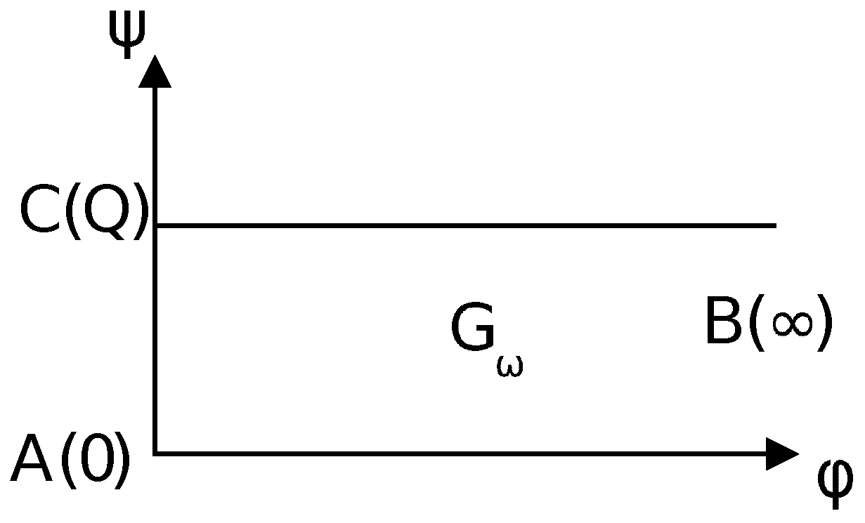
Let us consider a filtration scheme corresponding to the problem of convective diffusion of pollution from rivers, canals, or surface storages of industrial effluents (Figure 1).

For this scheme, the domain of complex flow potential $G_{\omega }$ has the form of a half-strip (Figure 2) and the solution of the corresponding filtration problem is given as [1] $x=H{e}^{\frac{\pi \phi }{2Q}}sin\left(\frac{\pi \psi }{2Q}\right)+\frac{\psi }{\kappa }$, $y=H{e}^{\frac{\pi \phi }{2Q}}cos\left(\frac{\pi \psi }{2Q}\right)+\frac{\phi }{\kappa }$ where $\kappa$ is the filtration coefficient, $Q=\kappa \left(\frac{L}{2}-H\right)$ is the filtration rate.

The problem of modeling pollutants migration in the right side $G_z$ of the symmetric filtration region (Figure 1) can be mathematically formulated as the problem of finding the solution of Equation (4) $((x,y,t)\in G_z\times (0,+\infty ))$ under the following boundary conditions: ${\left.C\right|}_{AC}=C_1,{\left.\frac{\partial C}{\partial n}\right|}_{AB,CB}=0,{\left.C\right|}_{t=0}=0$ where $C_1$ is the given concentration of soluble substances on filtration inflow, n is the outer normal to the corresponding line.

As the filtration domain $G_z$ is a domain with a partially unknown boundary, we make a transition to the variables $(\phi ,\psi )$ that represent the points of the domain $G_{\omega }=\left\{(\phi ,\psi ):0<\phi <+\infty ,0<\psi <Q\right\}$ (Figure 2). Finally, the boundary value problem in the domain of complex flow potential is as follows:

$$\sigma {}^k{D}_t^{\alpha }C={\upsilon }^2(\phi ,\psi )\left(d\left(\frac{{\partial }^{2}C}{\partial {\phi }^2}+\frac{{\partial }^{2}C}{\partial {\psi }^2}\right)-\frac{\partial C}{\partial \phi }\right)((\phi ,\psi ,t)\in G_{\omega }\times (0,+\infty )),$$

(5)

$${\left.C\right|}_{AC}=C_1,{\left.\frac{\partial C}{\partial \psi }\right|}_{AB,CB}=0,{\left.C\right|}_{t=0}=0.$$

(6)

We solve the considered problem under the following restrictions on the parameters of the derivative: $0<\alpha <1,k>1-\alpha$. It is easy to show that in this case we have

$${}^k{D}_t^{\alpha }C=\frac{1}{k^{1-\beta }}{D}_t^{(\beta )}C$$

where $D_t^{(\beta )}$ is the operator of the standard Caputo derivative of order $\beta$ with respect to the variable t [5,6,7,8], $\beta =\frac{k+\alpha -1}{k}(0<\beta <1)$. Then, Equation (5) can be rewritten as

$$\sigma D_t^{(\beta )}C\left(\phi ,\psi ,t\right)={\tilde{\upsilon }}^2(\phi ,\psi )\left(d\left(\frac{{\partial }^{2}C}{\partial {\phi }^2}+\frac{{\partial }^{2}C}{\partial {\psi }^2}\right)-\frac{\partial C}{\partial \phi }\right)$$

(7)

where ${\tilde{\upsilon }}^2(\phi ,\psi )=k^{1-\beta }{\upsilon }^2(\phi ,\psi )$ and the simulation of the dynamics of the considered anomalous convective diffusion process reduces to the solution of the boundary value problem for Equation (7) with the conditions (6) in the domain of complex flow potential.

Let us introduce the following dimensionless variables and parameters:

$$x^{\prime }=\frac{x}{L},y^{\prime }=\frac{y}{L},{\phi }^{\prime }=\frac{\phi }{Q},{\psi }^{\prime }=\frac{\psi }{Q},H^{\prime }=\frac{H}{L},C^{\prime }=\frac{C}{C_1},$$

$$d^{\prime }=\frac{d}{Q},\widetilde{{\upsilon }^{\prime }}=\frac{\tilde{\upsilon }}{{\upsilon }_0},t^{\prime }={\left(\frac{{\upsilon }_0^2}{Q}\right)}^{\frac{1}{\beta }}t,{\kappa }_1^{\prime }=\frac{2Q}{\pi \kappa H},{\kappa }^{\prime }=\frac{\kappa L}{Q},a^{\prime }={\left(\frac{Q}{{\upsilon }_{0}H}\right)}^2$$

(8)

where L is the parameter of scale, ${\upsilon }_0$ is the characteristic parameter of velocity.

Performing transition to the dimensionless variables (8) in (7), (6) (further dropping the prime sign over the dimensionless variables), we obtain in the domain $G_{\omega }\times (0,+\infty )$ the boundary value problem

$$\sigma D_t^{(\beta )}C(\phi ,\psi ,t)={\tilde{\upsilon }}^2(\phi ,\psi )\left(d\left(\frac{{\partial }^{2}C}{\partial {\phi }^2}+\frac{{\partial }^{2}C}{\partial {\psi }^2}\right)-\frac{\partial C}{\partial \phi }\right),$$

(9)

$$C(0,\psi ,t)=1,\frac{\partial C(\phi ,0,t)}{\partial \psi }=0,\frac{\partial C(\phi ,1,t)}{\partial \psi }=0,C(\phi ,\psi ,0)=0$$

(10)

where

$${\tilde{\upsilon }}^2(\phi ,\psi )=\frac{4a}{{\pi }^2}{k}^{1-\beta }\left(\frac{1}{e^{\pi \phi }{sin}^2\left(\frac{\pi \psi }{2}\right)}+\frac{1}{{\left(e^{\frac{\pi \phi }{2}}cos\left(\frac{\pi \psi }{2}\right)+{\kappa }_1\right)}^2}\right).$$

The transition from the domain of complex flow potential (Figure 2) to the physical domain (Figure 1) is carried out using the following formulas:

$$x=H{e}^{\frac{\pi \phi }{2}}sin\left(\frac{\pi \psi }{2}\right)+\frac{\psi }{\kappa },y=H{e}^{\frac{\pi \phi }{2}}cos\left(\frac{\pi \psi }{2}\right)+\frac{\phi }{\kappa }.$$

(11)

3. Approximate Solution of the Boundary Value Problem

In this section we present a finite-difference method for obtaining an approximate solution of the boundary value problem (9), (10).

Let us introduce the grid domain

$${\omega }_{h\tau }=\{({\phi }_i,{\psi }_k,t_j):{\phi }_i=i{h}_1(i=\overline{0,m+1}),{\psi }_k=h_2(k-0,5)(k=\overline{0,n+1}),$$

$$t_j=j\tau (j=\overline{0,N+1})\}$$

where $h_1=\frac{2{\phi }_0}{2m+1},h_2=\frac{1}{n}$ are the grid steps with respect to the geometric variables $\phi$, $\psi$; $\tau$ is the grid step with respect to the time variable; ${\phi }_0=const.$

Restricting the domain of complex flow potential from the right by the line $\phi ={\phi }_0({\phi }_0\gg 1)$ and posing an additional boundary condition on it (for example, the Neumann condition), we associate with the considered boundary value problem the following locally one-dimensional finite-difference scheme [14,29]:

$$\frac{\sigma }{2}{\Delta }_t^{(\beta )}\overline{C}={\tilde{\upsilon }}^2(d{\overline{C}}_{\overline{\phi }\phi }-{\overline{C}}_{\stackrel{0}{\phi }}),$$

(12)

$$\frac{\sigma }{2}{\Delta }_t^{(\beta )}\widehat{C}={\tilde{\upsilon }}^{2}d{\widehat{C}}_{\overline{\psi }\psi }$$

(13)

where $\widehat{C}=C^{j+1},\overline{C}=C^{j+\frac{1}{2}},C=C^j,t_{j+\frac{1}{2}}=t_j+\frac{\tau }{2}$, ${\overline{C}}_{\overline{\phi }\phi }=({\overline{C}}_{i+1,k}-2{\overline{C}}_{i,k}+{\overline{C}}_{i-1,k})/h_1^2$, ${\overline{C}}_{\stackrel{0}{\phi }}=\frac{{\overline{C}}_{i+1,k}-{\overline{C}}_{i-1,k}}{2h_1}$, ${\widehat{C}}_{\overline{\psi }\psi }=({\widehat{C}}_{i,k+1}-2{\widehat{C}}_{i,k}+{\widehat{C}}_{i,k-1})/h_2^2$, ${\Delta }_t^{(\beta )}\overline{C},{\Delta }_t^{(\beta )}\widehat{C}$ are the finite-difference counterpart of the fractional differentiation operator defined as

$${\Delta }_t^{(\beta )}\overline{C}=\frac{1}{\mathsf{\Gamma }(2-\beta )}\left[{\left(\frac{2}{\tau }\right)}^{\beta }\left(\overline{C}-C\right)+\sum _{s=0}^{j-1}{b}_s^{(j)}{C}_{t,s}\right],$$

$${\Delta }_t^{(\beta )}\widehat{C}=\frac{1}{\mathsf{\Gamma }(2-\beta )}\left\{\sum _{s=0}^{j-1}{\rho }_s^{(j)}{C}_{t,s}+{\left(\frac{2}{\tau }\right)}^{\beta }\left[\widehat{C}-C+2^{1-\beta }\left(\overline{C}-C\right)\right]\right\},$$

$$b_s^{(j)}={\tau }^{1-\beta }\left[{\left(j-s+\raisebox{1ex}{$1$}\!\left/ \!\raisebox{-1ex}{$2$}\right.\right)}^{1-\beta }-{\left(j-s-\raisebox{1ex}{$1$}\!\left/ \!\raisebox{-1ex}{$2$}\right.\right)}^{1-\beta }\right],{\rho }_s^{(j)}={\tau }^{1-\beta }\left[{\left(j-s+1\right)}^{1-\beta }-{\left(j-s\right)}^{1-\beta }\right]$$

where $C_{t,s}=\frac{C^{s+1}-C^s}{\tau }$, $\mathsf{\Gamma }(\alpha )$ is the Gamma function [30].

Let us note that in the class of sufficiently smooth functions we have the following error estimate:

$$D_t^{(\beta )}u={\Delta }_t^{(\beta )}u+O(\tau ).$$

Unrolling the finite-difference operators in (12) and collecting similar terms, we obtain on the half-integer step $t_{j+\frac{1}{2}}$ the following series of systems of linear algebraic equations

$$A_{il}{C}_{i+1,l}^{j+\frac{1}{2}}-B_{il}{C}_{il}^{j+\frac{1}{2}}+S_{il}{C}_{i-1,l}^{j+\frac{1}{2}}={\mathsf{\Phi }}_{il}^j(i=\overline{1,m};l=\overline{1,n};j=\overline{0,N})$$

(14)

where

$$A_{il}=\frac{{\tilde{\upsilon }}_{il}^2}{h_1}\left(\frac{d}{h_1}-0.5\right),S_{il}=\frac{{\tilde{\upsilon }}_{il}^2}{h_1}\left(\frac{d}{h_1}+0.5\right),B_{il}=\frac{\sigma }{2^{1-\beta }{\tau }^{\beta }\mathsf{\Gamma }(2-\beta )}+A_{il}+S_{il},$$

$${\mathsf{\Phi }}_{il}^j=\frac{\sigma }{2\mathsf{\Gamma }(2-\beta )}\left(\sum _{s=0}^{j-1}{b}_s^{(j)}\frac{C_{il}^{s+1}-C_{il}^s}{\tau }-{\left(\frac{2}{\tau }\right)}^{\beta }{C}_{il}^j\right).$$

The solution of the system (14) can be found by the Thomas algorithm as

$$C_{il}^{j+\frac{1}{2}}={\alpha }_{i+1,l}{C}_{i+1,l}^{j+\frac{1}{2}}+{\beta }_{i+1,l}^j(i=\overline{1,m};l=\overline{1,n};j=\overline{0,N})$$

(15)

where

$${\alpha }_{i+1,l}=\frac{A_{il}}{B_{il}-S_{il}{\alpha }_{il}},{\beta }_{i+1,l}^j=\frac{{\alpha }_{i+1,l}}{A_{il}}(S_{il}{\beta }_{il}^j-{\mathsf{\Phi }}_{il}^j)(i=\overline{1,m};l=\overline{1,n};j=\overline{0,N}).$$

We obtain the following starting values of the coefficients $\alpha ,\beta$ using the finite-difference counterpart $C_{0l}^j=1$ of the boundary condition in the point $\phi =0$:

$${\alpha }_{1l}=0,{\beta }_{1l}^j=1(l=\overline{1,n};j=\overline{0,N}).$$

From the finite-difference counterpart $C_{ml}^{j+\frac{1}{2}}=C_{m+1,l}^{j+\frac{1}{2}}(l=\overline{1,n};j=\overline{0,N})$ of the second-order boundary condition in the point $\phi ={\phi }_0$ using (15) we have

$$C_{m+1,l}^{j+\frac{1}{2}}=\frac{{\beta }_{m+1,l}^j}{1-{\alpha }_{m+1,l}}(l=\overline{1,n};j=\overline{0,N}).$$

After obtaining the solution on a half-integer time step, on an integer time step from (13) we obtain

$$P_{il}{C}_{i,l+1}^{j+1}-Q_{il}{C}_{il}^{j+1}+P_{il}{C}_{i,l-1}^{j+1}={\mathsf{\Omega }}_{il}^j(i=\overline{1,m};l=\overline{1,n;}j=\overline{0,N})$$

(16)

where

$$P_{il}=\frac{{\tilde{\upsilon }}_{il}^{2}d}{h_2^2},Q_{il}=\frac{\sigma }{2^{1-\beta }{\tau }^{\beta }\mathsf{\Gamma }(2-\beta )}+2P_{il},$$

$${\mathsf{\Omega }}_{il}^j=\frac{\sigma }{2\mathsf{\Gamma }(2-\beta )}\left\{\sum _{s=0}^{j-1}{\rho }_s^{(j)}\frac{C_{il}^{s+1}-C_{il}^s}{\tau }+{\left(\frac{2}{\tau }\right)}^{\beta }\left[2^{1-\beta }{C}_{il}^{j+\frac{1}{2}}-(1+2^{1-\beta })C_{il}^j\right]\right\}.$$

The solution of the system (16) can be found as

$$C_{il}^{j+1}={\tilde{\alpha }}_{i,l+1}{C}_{i,l+1}^{j+1}+{\tilde{\beta }}_{i,l+1}^j(i=\overline{1,m};l=\overline{1,n};j=\overline{0,N})$$

where

$${\tilde{\alpha }}_{i,l+1}=\frac{P_{il}}{Q_{il}-P_{il}{\tilde{\alpha }}_{il}},{\tilde{\beta }}_{i,l+1}^j={\tilde{\alpha }}_{i,l+1}\left({\tilde{\beta }}_{il}^j-\frac{{\mathsf{\Omega }}_{il}^j}{P_{il}}\right)(i=\overline{1,m};l=\overline{1,n};j=\overline{0,N}).$$

Taking into account the finite-difference form $C_{i0}^{j+1}=C_{i1}^{j+1}$$(i=\overline{1,m};j=\overline{0,N})$ of the boundary condition at $\phi =0$ we obtain the following starting values of the coefficients:

$${\tilde{\alpha }}_{i1}=1,{\tilde{\beta }}_{i1}^j=0(i=\overline{1,m};j=\overline{0,N})$$

and considering $C_{in}^{j+1}=C_{i,n+1}^{j+1}$$(i=\overline{1,m};j=\overline{0,N})$ we get

$$C_{i,n+1}^{j+1}=\frac{{\tilde{\beta }}_{i,n+1}^j}{1-{\tilde{\alpha }}_{i,n+1}}(i=\overline{1,m};j=\overline{0,N}).$$

These relationships make it possible to compute the solution on an integer time step.

On each step of the solution procedure, we have series of three-diagonal linear systems that are independent and, in the case of large grids, can be efficiently solved in parallel. As we consider a time-fractional model, the biggest impact on computational complexity of the scheme has the computation of the right-hand side vectors ${\mathsf{\Phi }}_{il}^j$ and ${\mathsf{\Omega }}_{il}^j$ that can be further optimized and parallelized. The stability of the Thomas algorithm for (14) and (16) follows from the fact of the diagonal predominance in the matrices of the coefficients of the linear systems and can be controlled by a proper choice of grid steps.

The subsequent transition to the physical domain is carried out according to (11).

4. Results of Numerical Experiments

Numerical modeling of the dynamics of solute migration using the considered non-classical model of convective diffusion is performed with respect to the dimensionless variables (8) for the input data from [26]. With the dimensionless time step equal to 0.1 we performed the simulation for the dimensionless time range $T\le 100$. Experimentally checking the convergence of the scheme, we solve the problem increasing the grid size starting from $50\times 50$. Maximal local relative error started changing not more than by 2. During the simulation, the time spent on computations on one step, as it is expected, increases from $t<10$ ms on the first step to $t=1820$ ms on the 1000-th time step. In the additional experiments, for the grid size equal to $30\times 30$ computation time on one step increase up to $t=90$ and for the grid size of $65\times 65$—up to $t=680$. The increase was linear for time steps less than 300, but become slightly non-linear in further computations. This effect can be explained by non-optimal cache usage [17]. Total computation time for the dimensionless time range $T\le 30$ quadratically depended on the grid size. For the grid size equal to 100 × 100, time spent on computing the right-hand side vectors became more than 90% of the total computation time starting from the 125-th time step, for the grid size of $65\times 65$—starting from the 231-th time step. For the smallest tested grid of 30 × 30 nodes, time spent on computing right-hand side vector became more than 80% of the total computation time starting from the 451-th time step.

Some of the obtained results are depicted in Figure 3, Figure 4 and Figure 5.

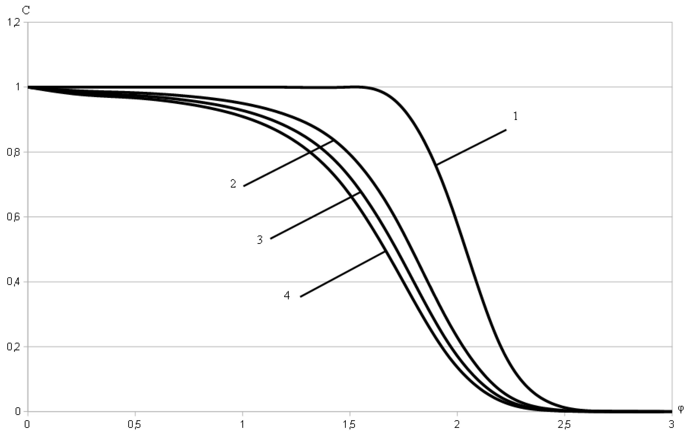
Figure 3 shows the changes in concentration field along the streamline $\psi =0.5$ at a fixed time $t=5$ depending on the value of the variable $\phi$ for the classical convective diffusion model (curve 1), the model with the standard Caputo derivative $D_t^{(\alpha )}C$ (curve 2, $\alpha =0.7$), and the model with the k-Caputo derivative ${}^k{D}_t^{\alpha }C$ (curves 3 and 4) for various values of the parameter k and a fixed value of order $\alpha =0.7$ (3 – $k=0.8$, 4 – $k=0.7$).

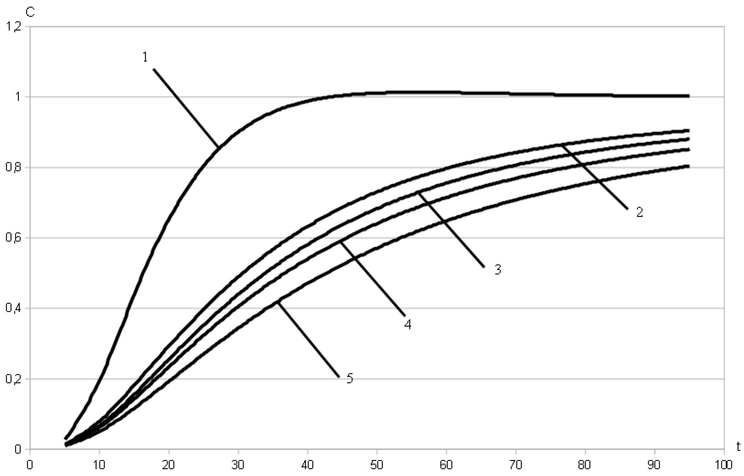
Figure 4 shows the growth pattern of the solute’s concentration at a fixed point of the filtration domain ($\phi =2.44,\psi =0.5$) depending on the value of the dimensionless time t: curve 1 corresponds to the classical model of convective diffusion, curve 2 corresponds to the model with the standard Caputo derivative $D_t^{(\alpha )}C$ for $\alpha =0.9$, curves 3–5 correspond to the model with the k-Caputo derivative (3 – $k=0.9$, 4 – $k=0.8$, 5 – $k=0.7$; $3,4,5$ – $\alpha =0.9$).

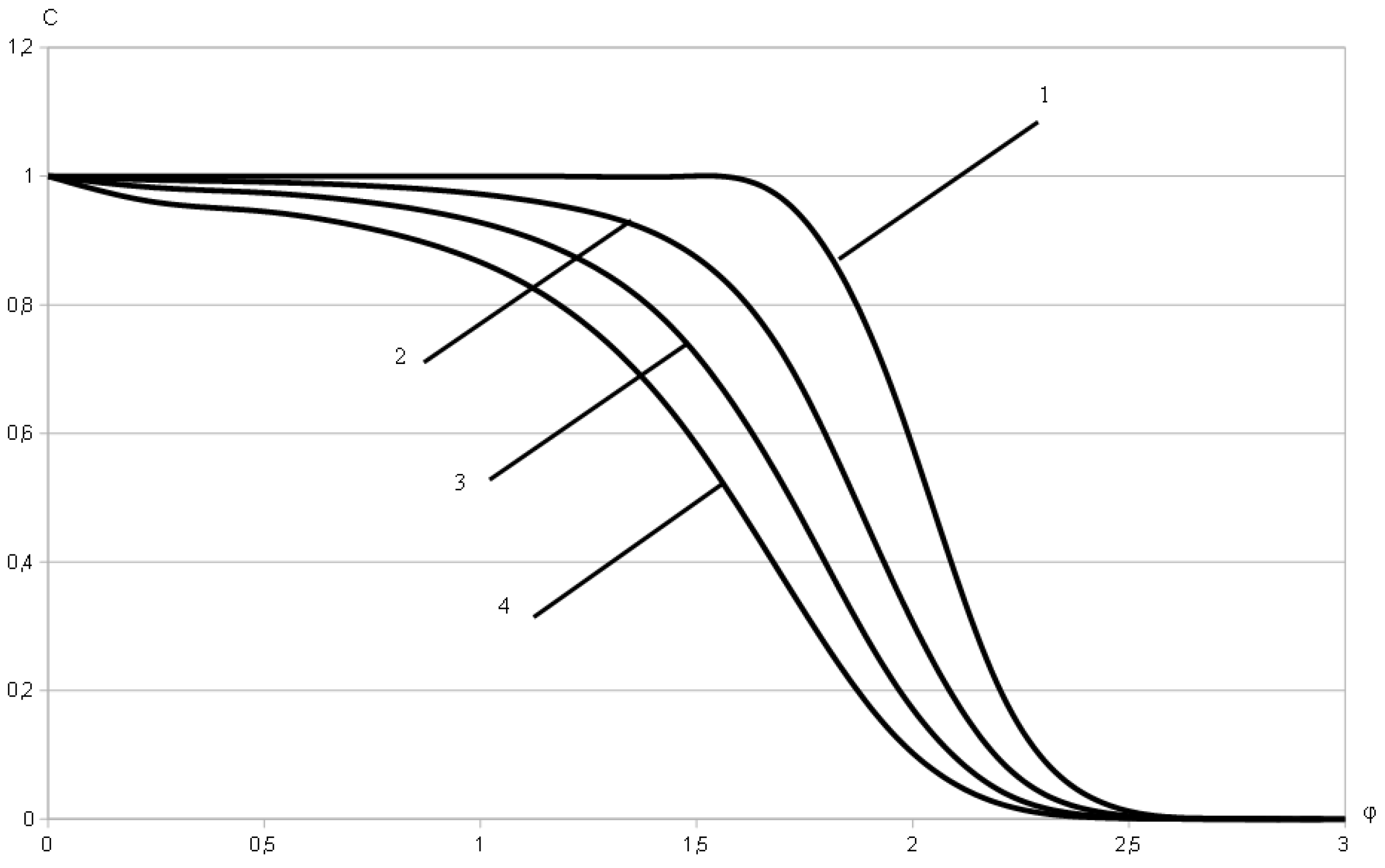
In Figure 5 we depict the changes in concentration field along the streamline $\psi =0.5$ at a fixed time $t=5$ subject to the values of the variable $\phi$ for the classical model (curve 1) and the model with the k-Caputo derivative ${}^k{D}_t^{\alpha }C$ (curves 2–4) for different values of order $\alpha$ and a fixed value of the parameter $k=0.8$ (2 – $\alpha =0.9$, 3 – $\alpha =0.8$,4 – $\alpha =0.7$).

The analysis of the results of the numerical experiments allows us to draw the following conclusions about the dynamics of solute concentration field modeled using the considered convective diffusion model:

• There is a delay in the formation of concentration field while modeling the diffusion process using the model with the k-Caputo derivative comparing both to the case of modeling this process using the classical model [1,2] and the model based on the standard definition of the Caputo derivative (Figure 3).
• For fixed values of order $\alpha$$(0<\alpha <1)$, when the value of the parameter k varies, this delay is the greater, the smaller the value of the parameter k is (Figure 3 and Figure 4).
• For fixed values of the parameter k, when the value of $\alpha$ varies, there is also a delay in the advance of concentration front for the diffusion model with the k-Caputo derivative compared with the case of the classical model. This delay is the greater, the smaller the value of the parameter $\alpha$ is (curves 2–4 in Figure 5). The performed computations also allow us to conclude that the dynamics of concentration front’s delay is determined to a greater extent by a change in the magnitude of order $\alpha$ than by a change of the value of the parameter k.

5. Conclusions

Consideration of a temporal non-locality of the convective diffusion in porous media with a complex internal structure on the base of the proposed model with the k-Caputo derivative opens the possibility of mathematical modeling of the phenomenon of a significant time lag in the process of diffusion field formation compared with the case when this process is described by the classical mathematical model or the model with the standard Caputo fractional derivative. Ignoring the phenomenon of a temporal non-locality of anomalous convective diffusion while developing engineering solutions (for example, in the field of designing systems for the environmentally safe operation of surface sewage storages in complex geological conditions) can lead to errors in forecasts of the degree of specified objects safety.