Adaptive Fractional-Order Sliding-Mode Control with Extended State Observer for Autonomous Underwater Vehicles Under Uncertain Disturbances

Abstract

In this paper, a composite control framework integrating feedback linearization, an extended state observer, and an adaptive fractional-order sliding-mode controller is presented for autonomous underwater vehicles operating under uncertain hydrodynamics and external disturbances. The proposed algorithm, named adaptive fractional-order sliding-mode control with extended state observer, aims to enhance trajectory-tracking accuracy, disturbance rejection, and robustness against model uncertainties beyond what is offered by conventional active disturbance rejection control and integer-order sliding-mode control. First, a fractional-order sliding surface with an extended state observer is introduced to estimate and compensate lumped disturbances, where the fractional operator provides intrinsic filtering and memory effects to reduce chattering. Second, an adaptive exponential reaching law with smooth switching is formulated to overcome the trade-off between convergence speed and chattering, and a Levant differentiator is employed for sensorless velocity estimation. Finally, the uniform ultimate boundedness of the closed-loop system is proved via Lyapunov stability theory. Comparative simulation studies on step, sinusoidal, and circular trajectories under external disturbances, measurement noise, and 50% parametric uncertainties demonstrate that the proposed controller achieves zero overshoot, suppresses position fluctuations by 97%, and reduces root mean square tracking errors by 38–70% relative to conventional methods, confirming its superior performance.

1. Introduction

Autonomous underwater vehicles (AUVs) exhibit high levels of autonomy and adaptability, making them an important research focus in ocean engineering and robotics. They are widely used in marine resource exploration [1], underwater environmental monitoring [2], underwater archaeology [3], and seabed topography mapping [4]. However, AUVs face numerous practical challenges. The underwater operating environment is complex and highly variable, hydrodynamic characteristics are strongly coupled, and nonlinear dynamics, fluid disturbances, parameter variations, and communication delays can significantly degrade control performance. Therefore, developing advanced control strategies capable of adapting to harsh underwater conditions and mitigating various disturbances is critical for enhancing operational reliability.

In the field of autonomous underwater vehicle (AUV) control, many robust trajectory-tracking methods have been proposed, such as backstepping [5], sliding-mode control (SMC) [6], adaptive control [7], model predictive control (MPC), neural networks [8], and observer-based techniques [9].

Recently, the control of autonomous marine vehicles has evolved toward higher levels of adaptiveness and intelligence. In particular, adaptive SMC for AUVs has been further developed to enhance robustness under strong coupling, nonlinear disturbances, and limited communication bandwidth. For example, Liu [10] proposed a neural-network-based adaptive SMC for AUV trajectory tracking that achieves real-time compensation of uncertainties through online parameter tuning. Li [11] developed an adaptive finite-time SMC for multirotor UAVs under stochastic wind disturbances, demonstrating improved transient response and reduced chattering. More recently, He [12] introduced a fractional-order sliding-mode observer combined with a cooperative control strategy for underactuated AUVs to achieve accurate path following in complex marine environments. Their method integrates fractional calculus and double-power convergence laws to enhance disturbance estimation, employs an adaptive gain adjustment to eliminate dependence on disturbance bounds, and utilizes a path-parameter-based formation coordination approach with low communication overhead. Simulation results verified that the proposed control scheme significantly improves path-following accuracy, formation maintenance, and disturbance suppression. These developments underscore the growing trend of integrating adaptive mechanisms, fractional calculus, and observer-based cooperative control techniques to achieve high-performance robust control for unmanned marine systems, motivating the development of the composite strategy presented in this work.

Zhang [13] proposed an adaptive backstepping sliding-mode controller for a fully actuated six-degree-of-freedom (6-DOF) AUV, where virtual velocity commands were generated through backstepping, and a sliding-mode term was used to address model uncertainties. To alleviate the “differential explosion” problem, Zheng [14] applied dynamic surface control to process the virtual velocity commands and adopted a radial basis function (RBF) neural network for disturbance compensation, ensuring the uniform ultimate boundedness of tracking errors. Qiao [15] designed an adaptive fast nonsingular terminal sliding-mode controller that introduces an adaptive mechanism into the integral sliding surface to estimate lumped uncertainties in real time, achieving exponential convergence of position-tracking errors.

Precise trajectory tracking and effective disturbance rejection are crucial for improving the accuracy and safety of AUV operations. Advances in static-model-based control of underwater robots [16,17] have enhanced robustness, while observer-based disturbance rejection techniques have attracted increasing attention. Liang [18] developed a finite-time observer based on a pseudo-rigid-body model to estimate acceleration for variable-impedance control and analyzed stability. Considering uncertainties and input saturation, Shao [19] combined an observer with SMC to compensate for model-error dynamics during trajectory tracking. Cao [20] unified internal uncertainties and external disturbances in continuum robots as generalized disturbances and suppressed them using an error-driven active disturbance rejection controller.

SMC [21] is valued for its strong disturbance rejection capability and engineering practicality. It drives system states to a sliding manifold in finite time, guaranteeing convergence to equilibrium. However, traditional SMC suffers from chattering due to high-frequency switching. Recently, fractional-order calculus has been increasingly applied in control, yielding promising results in systems such as permanent magnet synchronous motors [22] and teleoperated robotics [23]. Fractional-order sliding-mode control (FOSMC) [24,25] has been proposed to mitigate chattering, while composite SMC combined with disturbance observers offers additional advantages [26]. In active disturbance rejection control (ADRC) [27], the extended state observer (ESO) [28,29] estimates and compensates total disturbances, including model uncertainties and unmodeled dynamics.

Motivated by the integration of sliding-mode and fractional-order theories in [30], this paper presents a composite control framework that combines feedback linearization, an ESO, an adaptive fractional-order sliding-mode controller, and a Levant differentiator. The proposed scheme, referred to as adaptive fractional-order sliding-mode control with an extended state observer (AFOSMC-ESO), achieves high-precision and robust AUV control under uncertain marine conditions.

The main contributions of this work are summarized as follows:

• Fractional-order sliding surface with ESO. Unlike conventional ESO-SMC methods that employ integer-order sliding surfaces, the proposed controller adopts a fractional-order surface. The fractional operator introduces intrinsic filtering and memory effects, significantly reducing chattering while ensuring rapid convergence.
• Adaptive gain reaching law with smooth switching. To overcome the trade-off between convergence speed and chattering in fixed-gain reaching laws, an adaptive exponential reaching law is formulated, where the gains are expressed as $k\left(t\right)=k_0+k_1\left|s\right|$ and $\epsilon \left(t\right)={\epsilon }_0+{\epsilon }_1\parallel {\widehat{h}}_3\parallel$. Furthermore, the discontinuous sign function $\mathrm{sign}\left(s\right)$ is replaced by a smooth form ${\displaystyle \frac{s}{\sqrt{s^2+{\delta }^2}}}$, effectively suppressing high-frequency oscillations.
• Sensorless velocity estimation using a Levant differentiator. Unlike most ESO-SMC frameworks that require direct velocity measurements, the proposed method employs a Levant differentiator to estimate first-order derivatives of desired trajectories and system states solely from position or attitude signals. This approach enhances practicality, reduces hardware cost, and improves noise immunity in demanding underwater environments.
• Unified feedback linearization and ESO structure. Instead of treating the ESO as an independent feedforward compensator, it is embedded within a feedback-linearization architecture. The known nonlinear terms are analytically canceled, allowing the ESO to estimate only the residual lumped disturbances. This design reduces observer bandwidth requirements and enhances robustness against measurement noise.

Comprehensive simulations on step, sinusoidal, and circular trajectories under external disturbances, measurement noise, and up to 50% parametric uncertainties demonstrate superior tracking accuracy, disturbance rejection, and chattering suppression compared with conventional ADRC, integer-order SMC, and FOSMC schemes.

The remainder of this paper is organized as follows. Section 2 introduces the AUV kinematic and dynamic models. Section 3 presents the design and stability analysis of the proposed AFOSMC-ESO algorithm. Section 4 details simulation results and performance evaluation. Section 5 concludes the paper and outlines future research directions.

2. AUV Motion Model

2.1. Definition of Motion Variables

Following the nomenclature recommended by the Society of Naval Architects and Marine Engineers (SNAME), the position, attitude, velocity, forces, and moments of the AUV in their respective coordinate frames are summarized in

Table 1. Definitions of AUV motion variables.

DOF	Motion	Force/Moment	Velocity/Rate	Position/Attitude
1	Surge	X	u	x
2	Sway	Y	v	y
3	Heave	Z	w	z
4	Roll	K	p	$\varphi$
5	Pitch	M	q	$\theta$
6	Yaw	N	r	$\psi$

. The position–attitude vector in the inertial frame is defined as

$$\eta ={({\eta }_1^T,{\eta }_2^T)}^T,{\eta }_1={(x,y,z)}^T,{\eta }_2={(\varphi ,\theta ,\psi )}^T$$

(1)

where ${\eta }_1$ represents the position vector consisting of the longitudinal $\left(x\right)$, lateral $\left(y\right)$, and vertical $\left(z\right)$ positions, and ${\eta }_2$ denotes the attitude vector composed of the roll $\left(\varphi \right)$, pitch $\left(\theta \right)$, and yaw $\left(\psi \right)$ angles.

The linear and angular velocity vectors in the body-fixed frame are given by

$$\nu ={({\nu }_1^T,{\nu }_2^T)}^T,{\nu }_1={(u,v,w)}^T,{\nu }_2={(p,q,r)}^T$$

(2)

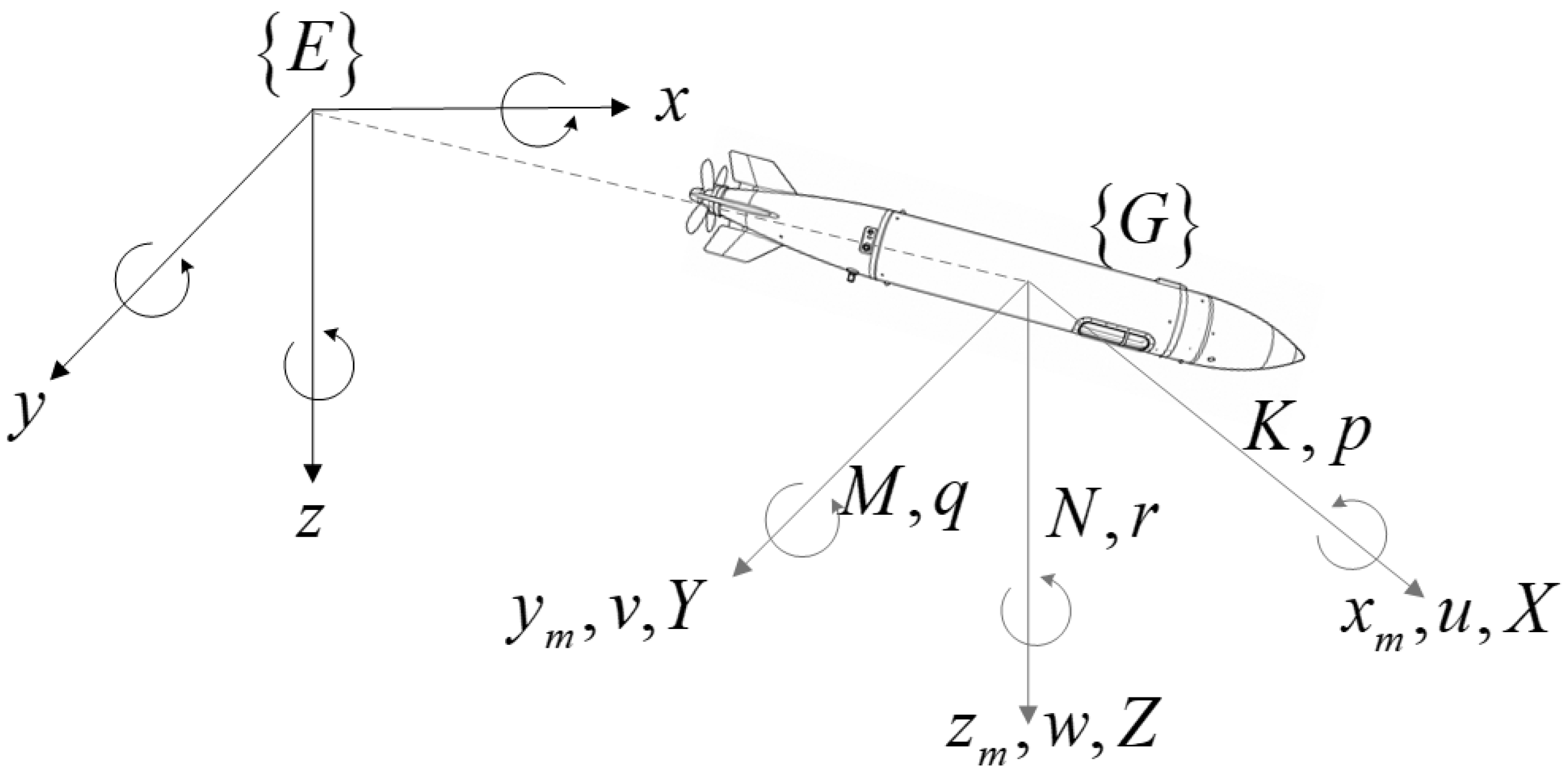
where ${\nu }_1$ contains the surge, sway, and heave velocities $(u,v,w)$, and ${\nu }_2$ contains the roll, pitch, and yaw rates $(p,q,r)$. The origin of the coordinate system is typically located at the AUV’s center, as illustrated in Figure 1.

2.2. AUV Model Formulation

Assuming the AUV is a rigid body with constant mass, the 6-DOF kinematic and dynamic equations in the inertial frame [31] can be expressed as

$$\left\{\begin{array}{cc}\hfill \dot{\eta }& =\mathbf{J}\left(\eta \right)\nu ,\hfill \\ \hfill \mathbf{M}\dot{\nu }+\mathbf{C}\left(\nu \right)\nu +\mathbf{D}\left(\nu \right)+\mathbf{g}\left(\eta \right)& ={\tau }_p+{\tau }_d\hfill \end{array}\right.$$

(3)

The total inertia matrix $\mathbf{M}$ consists of the rigid-body inertia ${\mathbf{M}}_{RB}$ and the added-mass matrix ${\mathbf{M}}_A$:

$$\mathbf{M}={\mathbf{M}}_{RB}+{\mathbf{M}}_A=\mathrm{diag}\{m_u,m_v,m_w,m_p,m_q,m_r\}$$

(4)

where $m_u=m-X_{\dot{u}}$, $m_v=m-Y_{\dot{v}}$, $m_w=m-Z_{\dot{w}}$, $m_p=I_x-K_{\dot{p}}$, $m_q=I_y-M_{\dot{q}}$, and $m_r=I_z-N_{\dot{r}}$. Here, $K_{\dot{p}},M_{\dot{q}},N_{\dot{r}},X_{\dot{u}},Y_{\dot{v}},Z_{\dot{w}}$ are the hydrodynamic inertia coefficients, and m is the AUV mass.

The centripetal and Coriolis matrix is expressed as

$$\begin{array}{cc}\hfill \mathbf{C}\left(\nu \right)& ={\mathbf{C}}_{RB}\left(\nu \right)+{\mathbf{C}}_A\left(\nu \right)=\hfill \\ \hfill & \left[\begin{array}{cccccc}0& 0& 0& 0& m_{v}v& -m_{v}v\\ 0& 0& 0& -m_{v}v& 0& m_{u}u\\ 0& 0& 0& m_{v}v& -m_{u}u& 0\\ 0& m_{v}v& -m_{v}v& 0& m_{r}r& -m_{q}q\\ -m_{v}v& 0& m_{u}u& -m_{r}r& 0& m_{p}p\\ m_{v}v& -m_{u}u& 0& m_{q}q& -m_{p}p& 0\end{array}\right]\hfill \end{array}$$

(5)

The hydrodynamic damping matrix is given by

$$\begin{array}{cc}\hfill \mathbf{D}\left(\nu \right)& =-\mathrm{diag}\{X_u,Y_v,Z_w,K_p,M_q,N_r\}\hfill \\ \hfill & -\mathrm{diag}\left\{X_{u\left|u\right|}\right|u|,Y_{v\left|v\right|}|v|,Z_{w\left|w\right|}|w|,K_{p\left|p\right|}|p|,M_{q\left|q\right|}|q|,N_{r\left|r\right|}|r\left|\right\}\hfill \end{array}$$

(6)

where $X_u,Y_v,Z_w,K_p,M_q,N_r$ are linear damping coefficients, and $X_{u\left|u\right|},Y_{v\left|v\right|},Z_{w\left|w\right|},K_{p\left|p\right|},M_{q\left|q\right|},N_{r\left|r\right|}$ are quadratic damping coefficients.

The restoring force and moment vector is expressed as

$$\mathbf{g}\left(\eta \right)=\left[\begin{array}{c}(G-B)sin\theta \\ -(G-B)cos\theta sin\varphi \\ -(G-B)cos\theta cos\varphi \\ y_{B}Bcos\theta cos\varphi -z_{B}Bcos\theta sin\varphi \\ -x_{B}Bcos\theta cos\varphi -z_{B}Bsin\theta \\ x_{B}Bcos\theta sin\varphi +y_{B}Bsin\theta \end{array}\right]$$

(7)

where $G=mg$ and $B=\rho gV$. Here, g is the gravitational acceleration, V is the displaced volume, and $\rho$ is the fluid density. The parameters $x_B$, $y_B$, and $z_B$ denote the coordinates of the buoyancy center relative to the center of gravity.

Considering model parameter uncertainties and external disturbances, the dynamic model can be rewritten as

$${\mathbf{M}}^{*}\dot{\nu }+{\mathbf{C}}^{*}\left(\nu \right)\nu +{\mathbf{D}}^{*}\left(\nu \right)\nu +{\mathbf{g}}^{*}\left(\eta \right)={\tau }_p+\mathbf{D}(\nu ,\dot{\nu })$$

(8)

where ${\mathbf{M}}^{*}=\mathbf{M}-\Delta \mathbf{M}$, ${\mathbf{C}}^{*}\left(\nu \right)=\mathbf{C}\left(\nu \right)-\Delta \mathbf{C}\left(\nu \right)$, ${\mathbf{D}}^{*}\left(\nu \right)=\mathbf{D}\left(\nu \right)-\Delta \mathbf{D}\left(\nu \right)$, and ${\mathbf{g}}^{*}\left(\eta \right)=\mathbf{g}\left(\eta \right)-\Delta \mathbf{g}\left(\eta \right)$. The superscript ${(·)}^{*}$ represents the nominal values obtained from computational fluid dynamics (CFD) simulations or experimental tests, while $\Delta (·)$ denotes the deviations from the actual parameters. The composite disturbance term

$$\mathbf{d}(\nu ,\dot{\nu })={\tau }_{um}+{\tau }_d=-\Delta \mathbf{M}\dot{\nu }-\Delta \mathbf{C}\left(\nu \right)\nu -\Delta \mathbf{D}\left(\nu \right)\nu -\Delta \mathbf{g}\left(\eta \right)+{\tau }_d$$

(9)

accounts for both model uncertainties $\left({\tau }_{um}\right)$ and external disturbances $\left({\tau }_d\right)$, such as ocean currents, waves, or tether interactions.

The transformation matrix $\mathbf{J}\left(\eta \right)$ relating the Earth-fixed and body-fixed coordinate frames is defined as

$$\mathbf{J}\left(\eta \right)=\left[\begin{array}{cccccc}{J}_{11}& J_{12}& J_{13}& 0& 0& 0\\ J_{21}& J_{22}& J_{23}& 0& 0& 0\\ J_{31}& J_{32}& J_{33}& 0& 0& 0\\ 0& 0& 0& 1& J_{45}& J_{46}\\ 0& 0& 0& 0& J_{55}& J_{56}\\ 0& 0& 0& 0& J_{65}& J_{66}\end{array}\right]$$

(10)

where

$$\begin{array}{cccc}\hfill & J_{11}=cos\psi cos\theta ,\hfill & \hfill & J_{12}=cos\psi sin\varphi sin\theta -cos\varphi sin\psi ,\hfill \\ \hfill & J_{13}=cos\psi cos\varphi sin\theta +sin\varphi sin\psi ,\hfill & \hfill & J_{21}=sin\psi cos\theta ,\hfill \\ \hfill & J_{22}=sin\psi sin\varphi sin\theta +cos\varphi cos\psi ,\hfill & \hfill & J_{23}=cos\psi sin\varphi sin\theta -sin\varphi cos\psi ,\hfill \\ \hfill & J_{31}=-sin\theta ,\hfill & \hfill & J_{32}=cos\theta sin\varphi ,J_{33}=cos\theta cos\varphi ,\hfill \\ \hfill & J_{45}=tan\theta sin\varphi ,\hfill & \hfill & J_{46}=tan\theta cos\varphi ,\hfill \\ \hfill & J_{55}=cos\varphi ,\hfill & \hfill & J_{56}=-sin\varphi ,\hfill \\ \hfill & J_{65}=sin\varphi /cos\theta ,\hfill & \hfill & J_{66}=cos\varphi /cos\theta .\hfill \end{array}$$

3. Controller Design

This section presents an FOSMC scheme augmented with an ESO. Through feedback linearization, the nonlinear dynamics are canceled, transforming the system into an equivalent linear form. The ESO estimates and compensates the total disturbance, which includes parameter uncertainties, unmodeled dynamics, and external perturbations. The FOSMC guarantees closed-loop stability, while the Levant differentiator provides accurate derivatives of the desired trajectory required for both linearization and control.

3.1. Problem Assumptions

To facilitate controller design and stability analysis while considering the practical operation characteristics of the AUV, the following assumptions [32] are made.

Assumption 1.

The desired pose trajectory ${\eta }_d$ and its first and second derivatives ${\dot{\eta }}_d$ and ${\ddot{\eta }}_d$ are known, bounded, and continuous.

Assumption 2.

The AUV attitude angles (roll ϕ, pitch θ, yaw ψ) satisfy $\left|\varphi \right|,\left|\theta \right|,\left|\psi \right|<{90}^{\circ }$ within the operating range. The coordinate transformation matrix $\mathit{J}\left(\eta \right)$ is nonsingular and bounded; that is, there exists a constant $J_{max}>0$ such that $\parallel \mathit{J}\left(\eta \right)\parallel \le J_{max}$ and ${\parallel \mathit{J}\left(\eta \right)}^{-1}\parallel \le J_{max}$.

Assumption 3.

The total disturbance ${\mathit{f}}_T=f_{um}+f_d$, including model uncertainties and external ocean disturbances, and its derivative ${\dot{\mathit{f}}}_T$ are bounded. There exist positive constants ${\delta }_1$ and ${\delta }_2$ such that

$$\parallel {\mathit{f}}_T\parallel \le {\delta }_1,\parallel {\dot{\mathit{f}}}_T\parallel \le {\delta }_2.$$

(11)

Assumption 4.

The output force/torque generated by the actuators is bounded. There exists ${\tau }_{max}>0$ such that $\parallel \tau \parallel \le {\tau }_{max}$.

3.2. Proposed Control Strategy

3.2.1. Control Model

Under the above assumptions, the dynamic model in Equation (8) is transformed into the inertial coordinate frame as

$${\mathit{M}}_{\eta }^{*}\ddot{\eta }+{\mathit{C}}_{\eta }^{*}(\nu ,\eta )\dot{\eta }+{\mathit{D}}_{\eta }^{*}(\nu ,\eta )\dot{\eta }+{\mathit{G}}_{\eta }^{*}\left(\eta \right)={\tau }_{\eta }+d_{\eta }(\nu ,\dot{\nu },\eta ).$$

(12)

Here, ${\mathit{M}}_{\eta }^{*}=\mathit{J}{\left(\eta \right)}^{-\mathrm{T}}{\mathit{M}}^{*}\mathit{J}{\left(\eta \right)}^{-1}$, ${\mathit{C}}_{\eta }^{*}(\nu ,\eta )=\mathit{J}{\left(\eta \right)}^{-\mathrm{T}}\left({\mathit{C}}^{*}-{\mathit{M}}^{*}\mathit{J}{\left(\eta \right)}^{-1}\dot{\mathit{J}}\right)\mathit{J}{\left(\eta \right)}^{-1}$, ${\mathit{G}}_{\eta }^{*}\left(\eta \right)=\mathit{J}{\left(\eta \right)}^{-\mathrm{T}}{\mathbf{g}}^{*}$, ${\mathit{D}}_{\eta }^{*}(\nu ,\eta )=\mathit{J}{\left(\eta \right)}^{-\mathrm{T}}{\mathit{D}}^{*}\mathit{J}{\left(\eta \right)}^{-1}$, ${\tau }_{\eta }=\mathit{J}{\left(\eta \right)}^{-\mathrm{T}}{\tau }_p$, and $d_{\eta }(\nu ,\dot{\nu },\eta )=\mathit{J}{\left(\eta \right)}^{-\mathrm{T}}({\tau }_{un}+{\tau }_d)$. The matrix ${\mathit{M}}_{\eta }^{*}$ is symmetric and positive definite. For any ${\alpha }_{\eta }\in {\mathbb{R}}^6$, ${\alpha }_{\eta }^{\mathrm{T}}({\dot{\mathit{M}}}_{\eta }^{*}-2{\mathit{C}}_{\eta }^{*}){\alpha }_{\eta }=0$ holds.

Accordingly, the control model of the AUV is expressed as

$$\ddot{\eta }={\mathit{M}}_{\eta }^{*-1}\left(\mathit{J}{\left(\eta \right)}^{-\mathrm{T}}{\tau }_p-{\mathit{C}}_{\eta }^{*}(\nu ,\eta )\dot{\eta }-{\mathit{D}}_{\eta }^{*}(\nu ,\eta )\dot{\eta }-{\mathit{G}}_{\eta }^{*}\left(\eta \right)\right)+f_{um}+f_d.$$

(13)

3.2.2. Feedback Linearization

Feedback linearization transforms the nonlinear system into a linear form using dynamic feedback. It is defined as

$${\tau }_1=\mathit{J}{\left(\eta \right)}^T\left({\mathit{C}}_{\eta }^{*}(\nu ,\eta )\dot{\eta }+{\mathit{D}}_{\eta }^{*}(\nu ,\eta )\dot{\eta }+{\mathit{G}}_{\eta }^{*}\left(\eta \right)\right).$$

(14)

Substituting (14) into (13) yields

$$\ddot{\eta }={\mathit{M}}_{\eta }^{*-1}\mathit{J}{\left(\eta \right)}^{-\mathrm{T}}{\tau }_c+{\mathit{f}}_{\mathrm{T}},$$

(15)

where ${\tau }_c={\tau }_p-{\tau }_1$ and ${\mathit{f}}_{\mathrm{T}}=f_{um}+f_d$ denotes the total disturbance.

3.2.3. Extended State Observer

To handle model uncertainties and external disturbances, an ESO is designed to estimate and compensate the total disturbance in real time. Let $h_1=\eta$, $h_2=\dot{\eta }$, $h_3={\mathit{f}}_{\mathrm{T}}$, then (15) becomes

$$\left\{\begin{array}{c}{\dot{h}}_1=h_2,\hfill \\ {\dot{h}}_2={\mathit{M}}_{\eta }^{*-1}\mathit{J}{\left(\eta \right)}^{-\mathrm{T}}{\tau }_c+h_3,\hfill \\ {\dot{h}}_3={\dot{f}}_{\mathrm{T}}.\hfill \end{array}\right.$$

(16)

The linear ESO is defined as

$$\left\{\begin{array}{c}{\dot{\widehat{h}}}_1={\widehat{h}}_2+{\beta }_1{e}_1,\hfill \\ {\dot{\widehat{h}}}_2={\widehat{h}}_3+{\mathit{M}}_{\eta }^{*-1}\mathit{J}{\left(\eta \right)}^{-\mathrm{T}}{\tau }_c+{\beta }_2{e}_1,\hfill \\ {\dot{\widehat{h}}}_3={\beta }_3{e}_1,\hfill \end{array}\right.$$

(17)

where $e_1=h_1-{\widehat{h}}_1$, ${\widehat{h}}_i\in {\mathbb{R}}^3$ are observer estimates, and ${\beta }_i\in \mathbb{R}$ are the observer gains.

The estimated total disturbance is compensated by

$${\tau }_2=-\mathit{J}{\left(\eta \right)}^T{\mathit{M}}_{\eta }^{*}{h}_3.$$

(18)

3.2.4. Adaptive Fractional-Order Sliding-Mode Controller

The fractional-order sliding-mode controller mitigates chattering and enhances transient response compared with conventional SMC designs. The sliding surface is defined as

$$s=\dot{e}+c_{1}e+c_2{D}^{\mu -1}e,$$

(19)

where $c_1,c_2>0$, $D^{\mu -1}$ denotes the fractional operator of order $\mu -1$ ($0<\mu <1$) under the Caputo definition, $e={\eta }_d-\eta$, and $\dot{e}={\dot{\eta }}_d-\dot{\eta }$.

Differentiating s gives

$$\dot{s}=\ddot{e}+c_1\dot{e}+c_2{D}^{\mu }e={\ddot{\eta }}_d-{\mathit{M}}_{\eta }^{*-1}\mathit{J}{\left(\eta \right)}^{-\mathrm{T}}{\tau }_3+c_1\dot{e}+c_2{D}^{\mu }e.$$

(20)

Fixed-gain exponential reaching laws often fail to balance convergence speed and chattering suppression. Large gains cause oscillations, while small gains slow convergence. To address this, an adaptive exponential law with a smooth nonlinear term is introduced:

$$\dot{s}=-k\left(t\right)s-\epsilon \left(t\right){\displaystyle \frac{s}{\sqrt{s^2+{\delta }^2}}}$$

(21)

where $k\left(t\right)=k_0+k_1\left|s\right|$, $\epsilon \left(t\right)={\epsilon }_0+{\epsilon }_1\left|{\widehat{h}}_3\right|$ ($k_0,k_1,{\epsilon }_0,{\epsilon }_1>0$) are predefined positive constants, and $\delta >0$ is a smoothing parameter. The adaptive gain $k\left(t\right)$ varies with $\left|s\right|$ to balance speed and robustness, while the smooth term ${\displaystyle \frac{s}{\sqrt{s^2+{\delta }^2}}}$ suppresses measurement noise.

Combining (20) with (21) gives the adaptive fractional-order sliding-mode control law:

$$\begin{array}{cc}\hfill {\tau }_3& =\mathit{J}{\left(\eta \right)}^{\mathrm{T}}{\mathit{M}}_{\eta }^{*}\left(c_1\dot{e}+c_2{D}^{\mu }e+{\ddot{\eta }}_d+k\left(t\right)s+\epsilon \left(t\right){\displaystyle \frac{s}{\sqrt{s^2+{\delta }^2}}}\right)\hfill \end{array}$$

(22)

3.2.5. Levant Differentiator

Accurate estimation of $\dot{\eta }$ is essential for the feedback linearization (14) and FOSMC (22). In practice, velocity measurement through sensors is costly and sensitive to noise, numerical differentiation is unstable, and model-based observers depend on accurate hydrodynamic parameters that are difficult to obtain.

The Levant differentiator overcomes these limitations and provides finite-time convergence with strong robustness. Its algorithm is expressed as

$$\left\{\begin{array}{c}{m}_1=-{\lambda }_1{|m_1-r|}^{3/4}\mathrm{sign}(m_1-r)+m_2,\hfill \\ m_2=-{\lambda }_2{|m_2-v_1|}^{2/3}\mathrm{sign}(m_2-v_1)+m_3,\hfill \\ m_3=-{\lambda }_3{|m_3-v_2|}^{1/2}\mathrm{sign}(m_3-v_2)+m_4,\hfill \\ {\dot{m}}_1=v_1,{\dot{m}}_2=v_2,{\dot{m}}_3=v_3,\hfill \\ {\dot{m}}_4=-{\lambda }_4\mathrm{sign}(m_4-v_3),\hfill \end{array}\right.$$

(23)

where r is the input signal, ${\lambda }_i$ are tunable parameters, and $m_i$ denote the estimated derivatives. The estimated $\dot{\eta }$ is replaced by $m_2$ in (14) and (22).

Finally, the overall control law is obtained as

$$\begin{array}{cc}\hfill \tau & ={\tau }_1+{\tau }_2+{\tau }_3\hfill \\ \hfill & =\mathit{J}{\left(\eta \right)}^T\left({\mathit{C}}_{\eta }^{*}(\nu ,\eta )\dot{\eta }+{\mathit{D}}_{\eta }^{*}(\nu ,\eta )\dot{\eta }+{\mathit{G}}_{\eta }^{*}\left(\eta \right)\right)\hfill \\ \hfill & +\mathit{J}{\left(\eta \right)}^T{\mathit{M}}_{\eta }^{*}\left(c_1\dot{e}+c_2{D}^{\mu }e+{\ddot{\eta }}_d+k\left(t\right)s+\epsilon \left(t\right){\displaystyle \frac{s}{\sqrt{s^2+{\delta }^2}}}-{\widehat{h}}_3\right).\hfill \end{array}$$

(24)

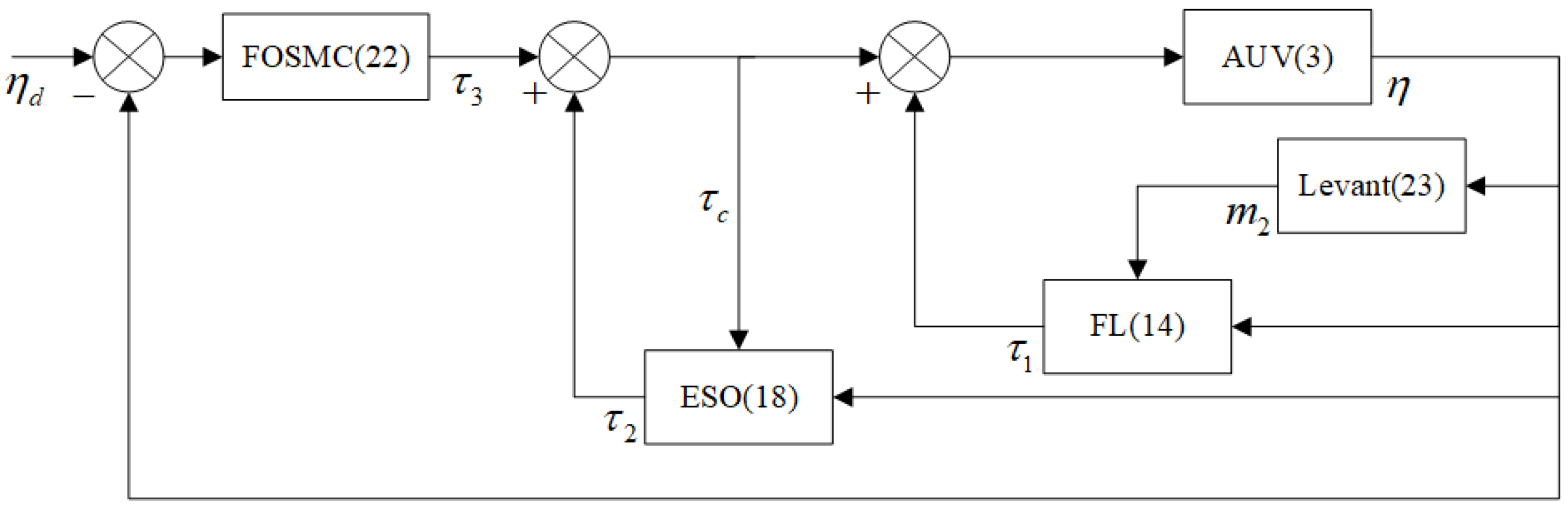
The block diagram of the proposed AUV control system based on ESO is shown in Figure 2.

3.3. Stability Analysis

This section rigorously establishes the stability of the proposed control strategy from two complementary perspectives: the ESO and the closed-loop system. Based on Lyapunov stability theory, it is shown that both the observer estimation error and the tracking error converge to bounded regions.

3.3.1. Stability Analysis of the ESO

To analyze the boundedness of the ESO estimation error, we define the observer error vector ${\mathit{e}}_{\mathrm{o}}={[e_1,e_2,e_3]}^T={[h_1-{\widehat{h}}_1,h_2-{\widehat{h}}_2,h_3-{\widehat{h}}_3]}^T$, where $h_1=\eta$, $h_2=\dot{\eta }$, and $h_3={\mathit{f}}_{\mathrm{T}}$ represent the augmented system states, while ${\widehat{h}}_1,{\widehat{h}}_2,{\widehat{h}}_3$ denote their corresponding ESO estimates. Here, $e_1$, $e_2$, and $e_3$ denote the position, velocity, and disturbance estimation errors, respectively. These collectively form the observer error vector ${\mathit{e}}_{\mathrm{o}}$, which is distinct from the tracking error analyzed later.

Differentiating ${\mathit{e}}_{\mathrm{o}}$ and substituting from (16)–(17) yields the ESO error dynamics:

$$\left\{\begin{array}{c}{\dot{e}}_1=e_2-{\beta }_1{e}_1,\hfill \\ {\dot{e}}_2=e_3-{\beta }_2{e}_1,\hfill \\ {\dot{e}}_3={\dot{\mathit{f}}}_{\mathrm{T}}-{\beta }_3{e}_1\hfill \end{array}\right.$$

(25)

In matrix form, this can be expressed as

$${\dot{\mathit{e}}}_{\mathrm{o}}=\mathit{A}{\mathit{e}}_{\mathrm{o}}+\mathit{B}{\dot{\mathit{f}}}_{\mathrm{T}},$$

(26)

where

$$\mathit{A}=\left[\begin{array}{ccc}-{\beta }_1& 1& 0\\ -{\beta }_2& 0& 1\\ -{\beta }_3& 0& 0\end{array}\right],\mathit{B}=\left[\begin{array}{c}0\\ 0\\ 1\end{array}\right].$$

(27)

The observer gains ${\beta }_1,{\beta }_2,{\beta }_3>0$ are chosen such that $\mathit{A}$ is Hurwitz, meaning all its eigenvalues have negative real parts.

For a Hurwitz matrix $\mathit{A}$, there exists a unique symmetric positive definite matrix $\mathit{P}$ satisfying

$${\mathit{A}}^T\mathit{P}+\mathit{P}\mathit{A}=-\mathit{Q},$$

(28)

where $\mathit{Q}$ is an arbitrary symmetric positive definite matrix.

Define the Lyapunov function as

$$V_1={\mathit{e}}_{\mathrm{o}}^T\mathit{P}{\mathit{e}}_{\mathrm{o}},$$

(29)

which is positive definite since $\mathit{P}>0$.

Differentiating $V_1$ and using (26) and (28) gives

$${\dot{V}}_1=-{\mathit{e}}_{\mathrm{o}}^T\mathit{Q}{\mathit{e}}_{\mathrm{o}}+2{\mathit{e}}_{\mathrm{o}}^T\mathit{P}\mathit{B}{\dot{\mathit{f}}}_{\mathrm{T}}.$$

(30)

From Assumption 3, ${\dot{\mathit{f}}}_{\mathrm{T}}$ is bounded, i.e., $\parallel {\dot{\mathit{f}}}_{\mathrm{T}}\parallel \le {\delta }_2$. Using $\parallel 2{\mathit{e}}_{\mathrm{o}}^T\mathit{P}\mathit{B}\parallel \le 2\parallel \mathit{P}\parallel \parallel \mathit{B}\parallel \parallel {\mathit{e}}_{\mathrm{o}}\parallel$ and defining $k_1=2\parallel \mathit{P}\parallel \parallel \mathit{B}\parallel {\delta }_2$, we have

$${\dot{V}}_1\le -{\lambda }_{min}\left(\mathit{Q}\right)\parallel {\mathit{e}}_{\mathrm{o}}{\parallel }^2+k_1\parallel {\mathit{e}}_{\mathrm{o}}\parallel .$$

(31)

Thus, ${\dot{V}}_1<0$ when $\parallel {\mathit{e}}_{\mathrm{o}}\parallel >k_1/{\lambda }_{min}\left(\mathit{Q}\right)$. According to Lyapunov’s ultimate boundedness theorem, ${\mathit{e}}_{\mathrm{o}}$ is uniformly ultimately bounded (UUB). Hence, $\parallel {\mathit{e}}_{\mathrm{o}}\parallel \le \mathrm{\Omega }$ as $t\to \infty$, for some $\mathrm{\Omega }>0$.

Therefore, the ESO effectively estimates the augmented system states, and the disturbance estimate ${\widehat{h}}_3$ tracks ${\mathit{f}}_{\mathrm{T}}$ within a bounded region.

Remark 1.

The above analysis confirms that ${\mathit{e}}_o$ is UUB. When ${\mathit{f}}_T$ varies slowly, the bound ${\delta }_2$ is small, leading to a tighter ultimate bound Ω. If ${\dot{\mathit{f}}}_T\to 0$, then $k_1\to 0$ and ${\dot{V}}_1=-{\mathit{e}}_o^T\mathit{Q}{\mathit{e}}_o<0$ for all ${\mathit{e}}_o\ne 0$. Thus, ${\mathit{e}}_o\left(t\right)$ converges asymptotically to zero in the absence of time-varying disturbances.

3.3.2. Stability Analysis of the Closed-Loop System

Since the proposed controller involves fractional-order terms defined in the Caputo sense, it is necessary to ensure that the Lyapunov-based stability framework remains valid. For $0<\mu <1$, the Caputo derivative $D^{\mu }{e}_{\eta }$ preserves the linearity and continuity properties required for Lyapunov analysis. Moreover, for systems $D^{\mu }x\left(t\right)=\mathit{A}x\left(t\right)$, asymptotic stability holds if and only if all eigenvalues ${\lambda }_i$ of $\mathit{A}$ satisfy $\left|arg\left({\lambda }_i\right)\right|>\mu \pi /2$.

In this work, $D^{\mu -1}{e}_{\eta }$ appears only in the sliding surface and not directly in the system dynamics, so the overall system remains of integer order. Thus, the classical Lyapunov method applies directly, while the fractional-order component influences transient response and robustness.

Define the tracking error as $e_{\eta }={\eta }_d-\eta$ and ${\dot{e}}_{\eta }={\dot{\eta }}_d-\dot{\eta }$. Consider the sliding surface

$$s={\dot{e}}_{\eta }+c_1{e}_{\eta }+c_2{D}^{\mu -1}{e}_{\eta },$$

(32)

where $c_1,c_2>0$ and $0<\mu <1$. Differentiating gives

$$\dot{s}={\ddot{e}}_{\eta }+c_1{\dot{e}}_{\eta }+c_2{D}^{\mu }{e}_{\eta }.$$

(33)

By substituting the system dynamics (15) and control law, one obtains

$$\dot{s}=-k\left(t\right)s-\epsilon \left(t\right){\displaystyle \frac{s}{\sqrt{s^2+{\delta }^2}}}+2{\tilde{h}}_3,$$

(34)

where ${\tilde{h}}_3={\widehat{h}}_3-h_3=-e_3$ is bounded with $\parallel {\tilde{h}}_3\parallel \le {\tilde{h}}_{max}$.

Select the Lyapunov candidate

$$V_2={\displaystyle \frac{1}{2}}{s}^{T}s.$$

(35)

Differentiating $V_2$ yields

$${\dot{V}}_2=-k\left(t\right){\parallel s\parallel }^2-\epsilon \left(t\right){\displaystyle \frac{{\parallel s\parallel }^2}{\sqrt{s^2+{\delta }^2}}}+2s^T{\tilde{h}}_3.$$

(36)

where $k\left(t\right)=k_0+k_1\parallel s\parallel$ and $\epsilon \left(t\right)={\epsilon }_0+{\epsilon }_1\parallel {\widehat{h}}_3\parallel$, with all gains positive, leads to

$${\dot{V}}_2\le -k_0{\parallel s\parallel }^2-k_1{\parallel s\parallel }^3-{\epsilon }_0{\displaystyle \frac{{\parallel s\parallel }^2}{\sqrt{{\parallel s\parallel }^2+{\delta }^2}}}-{\epsilon }_1\parallel {\widehat{h}}_3\parallel {\displaystyle \frac{{\parallel s\parallel }^2}{\sqrt{{\parallel s\parallel }^2+{\delta }^2}}}+2\parallel s\parallel {\tilde{h}}_{max}.$$

(37)

When $\parallel s\parallel \ge 4{\tilde{h}}_{max}/k_0$, ${\dot{V}}_2\le -{\displaystyle \frac{k_0}{2}}{\parallel s\parallel }^2<0$. Therefore, s is UUB, implying that the tracking error is bounded.

Remark 2.

Since ${\tilde{h}}_3$ is bounded, s remains UUB. If ${\tilde{h}}_3\to 0$, then ${\dot{V}}_2=-k\left(t\right){\parallel s\parallel }^2-\epsilon \left(t\right){\displaystyle \frac{{\parallel s\parallel }^2}{\sqrt{s^2+{\delta }^2}}}<0$ for any $s\ne 0$, guaranteeing $s\to 0$ and $e\to 0$ asymptotically when no disturbance exists.

3.3.3. Interaction Between the ESO and the Sliding-Mode Controller

Although the ESO and SMC are analyzed separately, their coupling must be considered because the disturbance estimate ${\widehat{h}}_3$ directly affects the control input. Substituting the ESO output into the sliding dynamics gives

$$\dot{s}=-k\left(t\right)s-\epsilon \left(t\right){\displaystyle \frac{s}{\sqrt{s^2+{\delta }^2}}}-2e_3,$$

(38)

where $e_3$ is the disturbance estimation error.

Consider the composite Lyapunov function

$$V=V_1+V_2={\mathit{e}}^T\mathit{P}\mathit{e}+{\displaystyle \frac{1}{2}}{s}^{T}s.$$

(39)

Differentiating gives

$$\dot{V}=-{\mathit{e}}^T\mathit{Q}\mathit{e}-k\left(t\right){\parallel s\parallel }^2-\epsilon \left(t\right){\displaystyle \frac{{\parallel s\parallel }^2}{\sqrt{s^2+{\delta }^2}}}+2{\mathit{e}}^T\mathit{P}\mathit{B}{\dot{\mathit{f}}}_{\mathrm{T}}-2s^T{e}_3.$$

(40)

Since $\parallel {\dot{\mathit{f}}}_{\mathrm{T}}\parallel \le {\delta }_2$ and $\parallel e_3\parallel \le \parallel \mathit{e}\parallel$, one obtains

$$\dot{V}\le -{\lambda }_{min}{\left(\mathit{Q}\right)\parallel \mathit{e}\parallel }^2-k_0{\parallel s\parallel }^2+{\kappa }_1\parallel \mathit{e}\parallel +{\kappa }_2\parallel s\parallel \parallel \mathit{e}\parallel ,$$

(41)

where ${\kappa }_1=2\parallel \mathit{P}\parallel \parallel \mathit{B}\parallel {\delta }_2$ and ${\kappa }_2$ is a positive constant. Hence, $\dot{V}$ is negative outside a compact set, implying that both $\mathit{e}$ and s are UUB.

Remark 3.

The composite Lyapunov function ensures that all closed-loop variables are UUB. When ${\dot{\mathit{f}}}_T\to 0$, $\dot{V}=-{\mathit{e}}^T\mathit{Q}\mathit{e}-k\left(t\right){\parallel s\parallel }^2-\epsilon \left(t\right){\displaystyle \frac{{\parallel s\parallel }^2}{\sqrt{s^2+{\delta }^2}}}<0$, ensuring asymptotic convergence of $\mathit{e}$ and s. Thus, the ESO-SMC structure guarantees joint stability and bounded convergence of all closed-loop signals.

4. Simulations and Experiments

In this section, the effectiveness of the proposed control strategy is validated through comparison with a conventional ADRC controller, an integer-order sliding-mode controller, and a conventional fractional-order controller. Three representative reference trajectories are considered in the simulations: a step input, a sinusoidal input, and a circular path. External disturbances and model uncertainties are also introduced. Based on the AUV dynamics described by (8), the system model is implemented using the MATLAB Function block in MATLAB/Simulink R2024b. The AUV model parameters follow [31], as listed in

Table 2. Main physical parameters of the AUV.

Parameter	Value	Unit
Dimensions	$380\times 267\times 165$	mm
Weight	55	N
Diving depth	100	m
Moments of inertia	$[0.12,0.25,0.2]$	kg·m2
Maximum speed	1.5	m/s

and

Table 3. Hydrodynamic coefficients of the AUV.

Parameter	Value	Parameter	Value
$X_u/\mathrm{kg}$	−2.61	$K_p/(\mathrm{kg}·{\mathrm{m}}^2·{\mathrm{rad}}^{-1})$	−0.15
$X_u/(\mathrm{N}·\mathrm{s}·{\mathrm{m}}^{-1})$	−2.47	$K_p/(\mathrm{N}·\mathrm{s}·{\mathrm{rad}}^{-1})$	−0.82
$X_{u\left|u\right|}/(\mathrm{N}·{\mathrm{s}}^2·{\mathrm{m}}^{-2})$	−8.33	$K_{p\left|p\right|}/(\mathrm{N}·{\mathrm{s}}^2·{\mathrm{rad}}^{-2})$	−2.95
$Y_v/\mathrm{kg}$	−5.56	$M_q/(\mathrm{kg}·{\mathrm{m}}^2·{\mathrm{rad}}^{-1})$	−0.26
$Y_v/(\mathrm{N}·\mathrm{s}·{\mathrm{m}}^{-1})$	−3.54	$M_q/(\mathrm{N}·\mathrm{s}·{\mathrm{rad}}^{-1})$	−0.90
$Y_{v\left|v\right|}/(\mathrm{N}·{\mathrm{s}}^2·{\mathrm{m}}^{-2})$	−10.82	$M_{q\left|q\right|}/(\mathrm{N}·{\mathrm{s}}^2·{\mathrm{rad}}^{-2})$	−3.67
$Z_w/\mathrm{kg}$	−9.75	$N_r/(\mathrm{kg}·{\mathrm{m}}^2·{\mathrm{rad}}^{-1})$	−0.21
$Z_w/(\mathrm{N}·\mathrm{s}·{\mathrm{m}}^{-1})$	−2.38	$N_r/(\mathrm{N}·\mathrm{s}·{\mathrm{rad}}^{-1})$	−0.45
$Z_{w\left|w\right|}/(\mathrm{N}·{\mathrm{s}}^2·{\mathrm{m}}^{-2})$	−14.13	$N_{r\left|r\right|}/(\mathrm{N}·{\mathrm{s}}^2·{\mathrm{rad}}^{-2})$	−1.56

. The AUV is assumed to be neutrally buoyant ($G\approx B$). Controller modules are constructed using Simulink libraries to comprehensively evaluate control performance. For reproducibility, the complete implementation of the AUV model, control algorithms, and simulation setup is available in the public GitHub repository at https://github.com/qianshiya/AFOSMCESO (accessed on 27 May 2026), which contains all MATLAB/Simulink files, parameter configurations, and documentation for replication and further research.

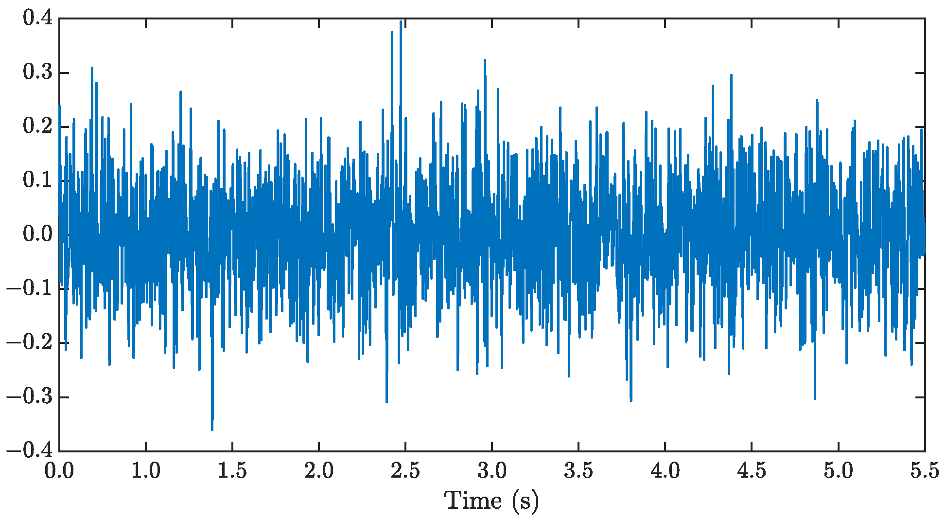
In this study, measurement noise is generated using the built-in white noise module in Simulink. A normalized and dimensionless noise signal is adopted to represent relative measurement perturbations instead of physical quantities. The same noise sequence is applied to all controllers to ensure fair comparison under identical disturbance conditions. The noise characteristics are illustrated in Figure 3. Furthermore, the main tuning parameters of all controllers are selected such that their closed-loop bandwidths are comparable, enabling objective evaluation of disturbance rejection and robustness.

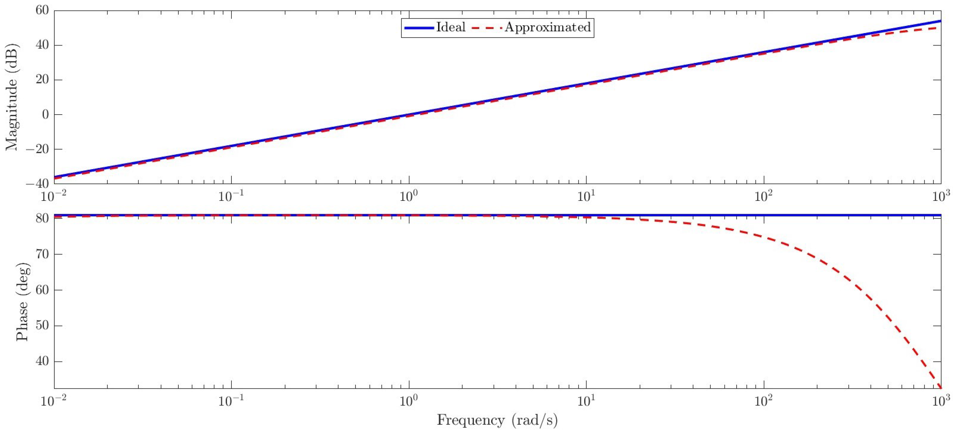
The procedure for parameter tuning is carried out as follows. Initially, the parameters of the fractional-order sliding-mode controller in the proposed scheme are set equal to those of the comparison sliding-mode controller, while the observer bandwidth of the proposed ESO is kept identical to that of the conventional ADRC observer. Subsequently, ${\omega }_c$ of the ADRC and the parameters of the integer-order sliding-mode controller are adjusted. The observer bandwidth ${\omega }_o$ must achieve a balance between disturbance rejection and noise sensitivity. An increase in ${\omega }_o$ improves disturbance rejection but also makes the system more susceptible to noise. As illustrated in Figure 4, a large ${\omega }_o$ results in noticeable discrepancies between the simulation and experimental results, whereas an excessively small value leads to prolonged regulation time. Considering these factors comprehensively, ${\omega }_o$ is selected as a trade-off. The final optimized controller parameters are summarized in

Table 4. Parameter settings of different controllers.

Controllers	Parameters
ADRC	${\omega }_c=50;{\omega }_o=50$
SMC	$c=50;k=5;\epsilon =1$
FOSMC	$c_1=50;c_2=1;k=5;\epsilon =1;\mu =0.9$
AFOSMC-ESO	$c_1=50;c_2=1;k_0=5;{\epsilon }_0=1;k_1=0.05;{\epsilon }_1=0.35;\mu =0.9;{\omega }_o=50$

.

In engineering applications, AUV dynamic parameters can be obtained via system identification, upon which the feedback-linearization term is designed. ESO parameters can then be determined using inertia matrix information, and fractional-order sliding-mode parameters are tuned to achieve desired dynamic performance. For comparison strategies, the feedback-linearization design is kept consistent across all controllers; integer-order SMC parameters are identical to those of the FOSMC in the proposed scheme, and ADRC observer parameters are the same as those used herein. By tuning ${\omega }_c$ and parameters of the conventional FOSMC, all control algorithms are evaluated under equivalent conditions.

Fractional-order calculus is implemented using the FOMCON toolbox in MATLAB. The Bode plot of the discrete approximation is compared with the true Bode plot in Figure 4.

4.1. Tracking Performance of the Levant Differentiator

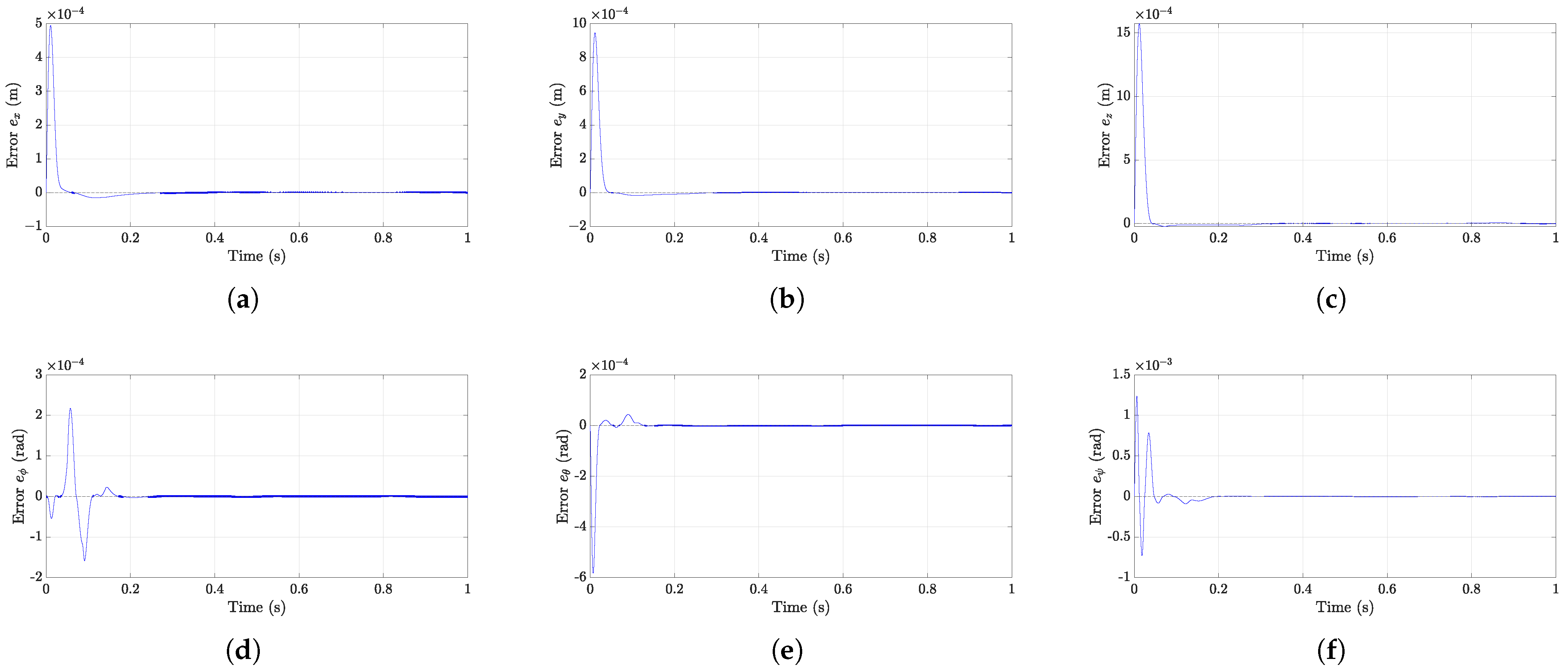
Using the established Levant differentiator model, the parameters ${\lambda }_1=810$, ${\lambda }_2=270$, ${\lambda }_3=90$, and ${\lambda }_4=30$ are selected for validation during circular-trajectory tracking. Figure 5 shows the estimation error of the six-degree-of-freedom signal $\eta$, representing the difference between the differentiator output and the actual signal.

The results indicate that the overall error range includes transient fluctuations during the start-up phase and is therefore relatively large. The steady-state error range reflects only minor fluctuations after stabilization and remains within the order of ${10}^{-3}$, demonstrating high accuracy. These findings verify that the proposed Levant differentiator achieves excellent tracking accuracy and robustness, satisfying the practical requirements of derivative estimation in control systems.

4.2. Step-Signal Tracking

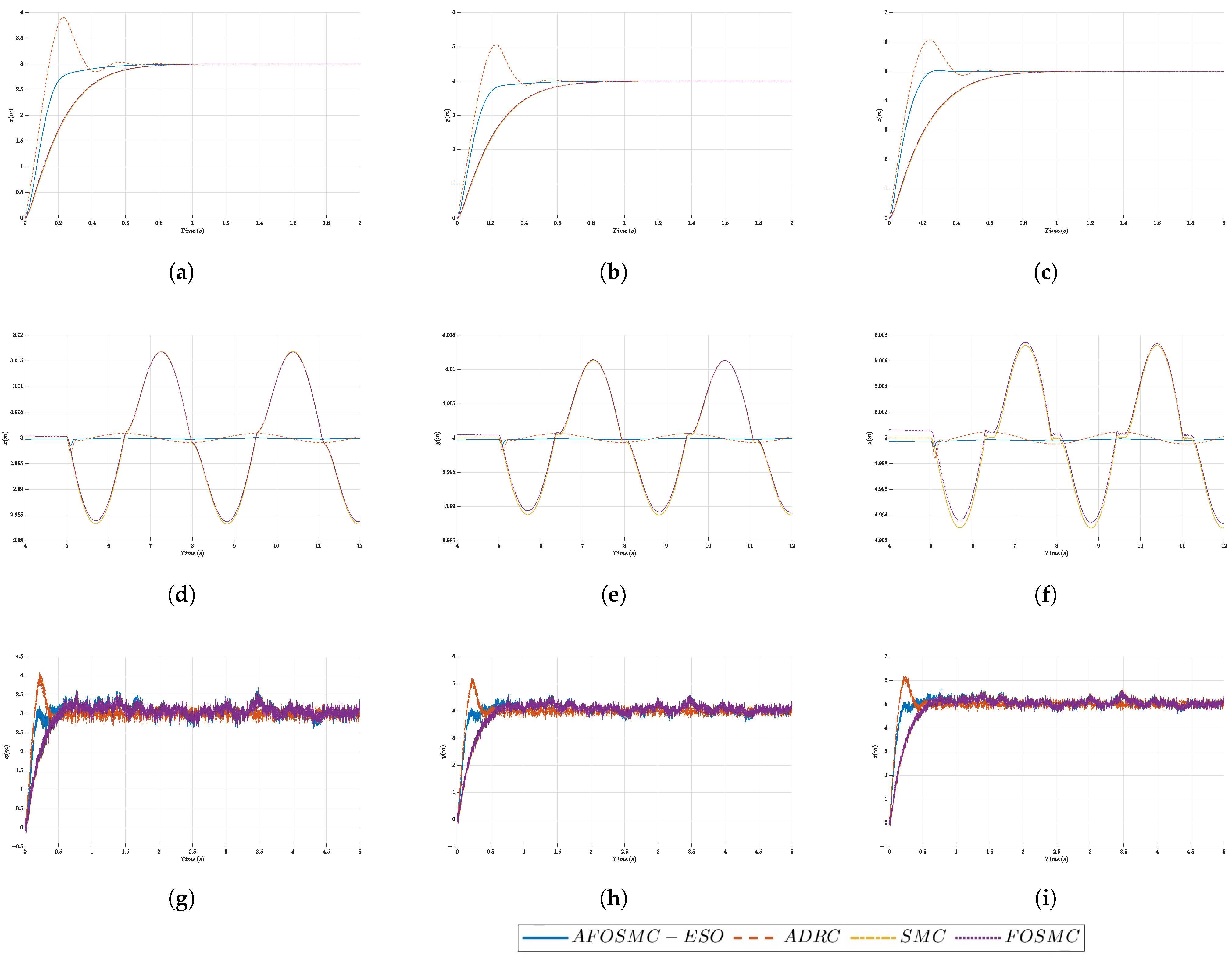
In the simulation, the AUV performs a 6-DOF motion, and the desired pose is defined as ${\eta }_d=(3,4,5,0^{\circ },0^{\circ },0^{\circ })$. The AUV starts from the origin with zero initial attitude angles. An uncertain external disturbance, represented by ${\tau }_d=90sintcost+30$, is introduced at $t=5\mathrm{s}$. The corresponding system responses are illustrated in Figure 6.

Table 5. Performance comparison of step responses with different controllers.

Controller	X-Axis			Y-Axis			Z-Axis
	OS (%)	ST (s)	FR (m)	OS (%)	ST (s)	FR (m)	OS (%)	ST (s)	FR (m)
AFOSMC-ESO	-	0.617	2.999∼3.000	-	0.584	3.999∼4.000	-	0.534	4.999∼5.000
ADRC	21.6	0.328	2.999∼3.001	19.8	0.240	3.999∼4.001	17.0	0.352	4.999∼5.000
FOSMC	0.5	0.679	2.985∼3.016	0.5	0.682	3.987∼4.013	0.5	0.684	4.994∼5.008
SMC	0.5	0.882	2.985∼3.019	0.5	0.888	3.987∼4.014	0.5	0.885	4.992∼5.008

summarizes the overshoot (OS), settling time (ST), and fluctuation range (FR) of the state variables within the interval 10∼12 s, whereas

Table 6. Performance comparison of responses under measurement noise.

Controller	Step			Sinusoidal
	X (m)	Y (m)	Z (m)	X (m)	Y (m)	Z (m)
AFOSMC-ESO	0.397	0.481	0.563	0.247	0.256	0.266
ADRC	0.310	0.391	0.466	0.253	0.335	0.821
FOSMC	0.486	0.644	0.793	0.387	0.307	0.271
SMC	0.492	0.651	0.806	0.401	0.308	0.268

presents the root mean square (RMS) values of each state under measurement noise conditions.

Assuming accurate knowledge of the AUV dynamics, the comparative performance of the four controllers can be described as follows. In terms of overshoot, the ADRC method exhibits the largest value of $21.6\%$. Both SMC and FOSMC achieve small overshoots of approximately $0.5\%$, whereas the proposed AFOSMC-ESO achieves a completely overshoot-free response. Regarding settling time, ADRC provides the fastest convergence at approximately $0.328\mathrm{s}$, followed by AFOSMC-ESO with $0.617\mathrm{s}$.

When external disturbances are applied, AFOSMC-ESO and ADRC achieve comparable fluctuation ranges, both outperforming SMC and FOSMC with FR values below $0.001$. As shown in Figure 6f, after the disturbance is introduced at $t=5\mathrm{s}$, the AFOSMC-ESO controller effectively confines the position fluctuations within $\pm 0.001\mathrm{m}$ and restores steady-state operation within approximately $0.3\mathrm{s}$, demonstrating the fastest disturbance rejection among all controllers. Although ADRC achieves a similar fluctuation amplitude, its recovery time is longer at approximately $0.6\mathrm{s}$. In contrast, SMC and FOSMC exhibit larger fluctuation amplitudes of $0.034\mathrm{m}$ and $0.031\mathrm{m}$, respectively, indicating inferior disturbance suppression. Furthermore, the AFOSMC-ESO controller exhibits no significant transient spike at the disturbance onset, which can be attributed to the rapid estimation and compensation of total disturbances by the ESO.

Under measurement noise, ADRC demonstrates the smallest overall noise level, whereas AFOSMC-ESO exhibits significantly stronger noise attenuation compared with the other methods.

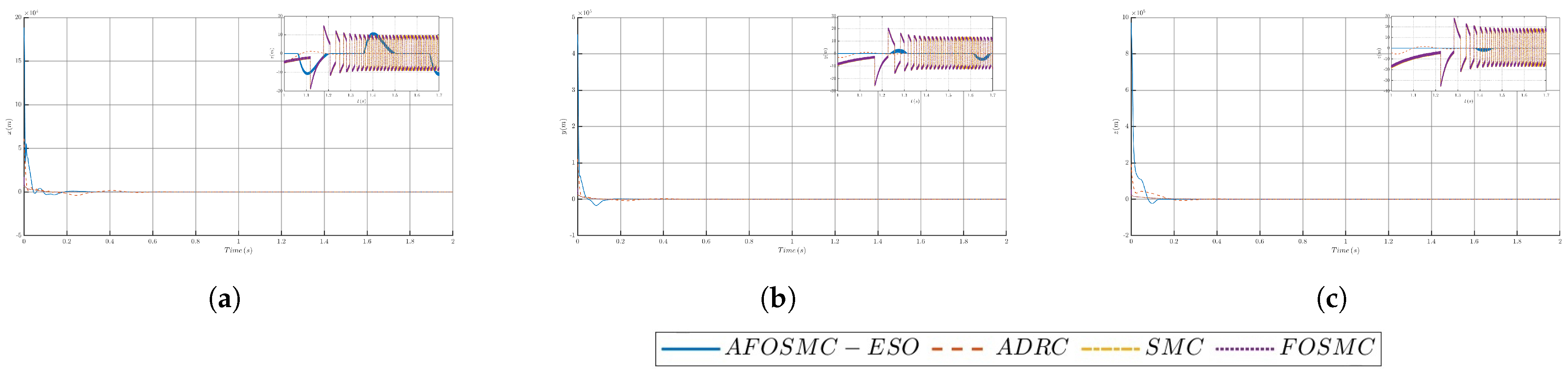
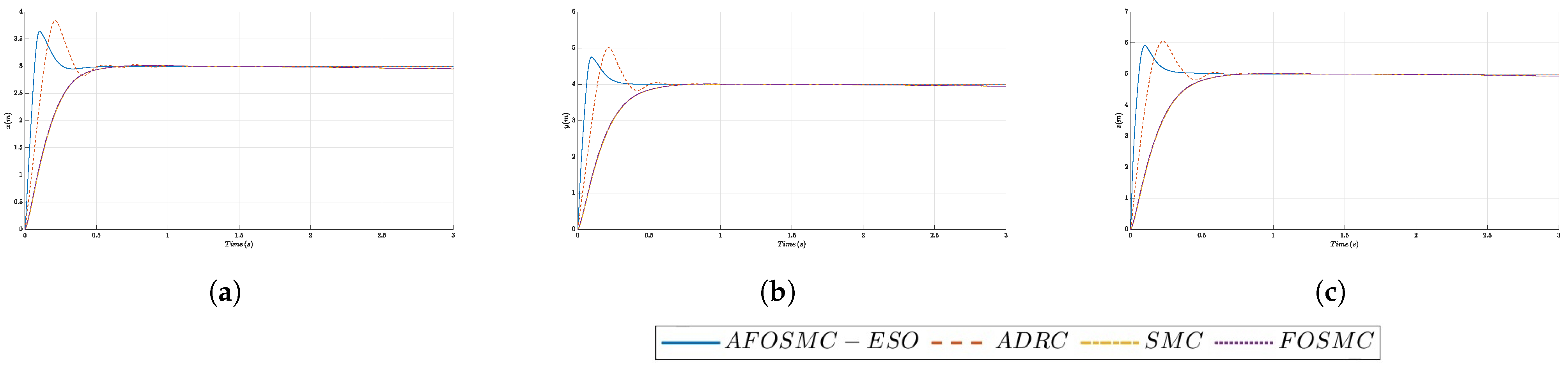
Figure 7 presents the control signals of different controllers during the time interval 0∼2 s. Due to its inherent characteristics, ADRC produces chattering-free control outputs, whereas the other three controllers display chattering to varying degrees. Among them, the proposed AFOSMC-ESO generates the mildest chattering. Furthermore, as illustrated in Figure 8, a sinusoidal disturbance of $3sin\left(t\right)$ is applied to the control force of each DOF to evaluate robustness. The results indicate that both AFOSMC-ESO and ADRC maintain small tracking errors under this condition, while SMC and FOSMC experience monotonically accumulating errors, reaching approximately $0.5\mathrm{m}$ for each of the three DOFs at $t=3\mathrm{s}$.

4.3. Sinusoidal-Signal Tracking

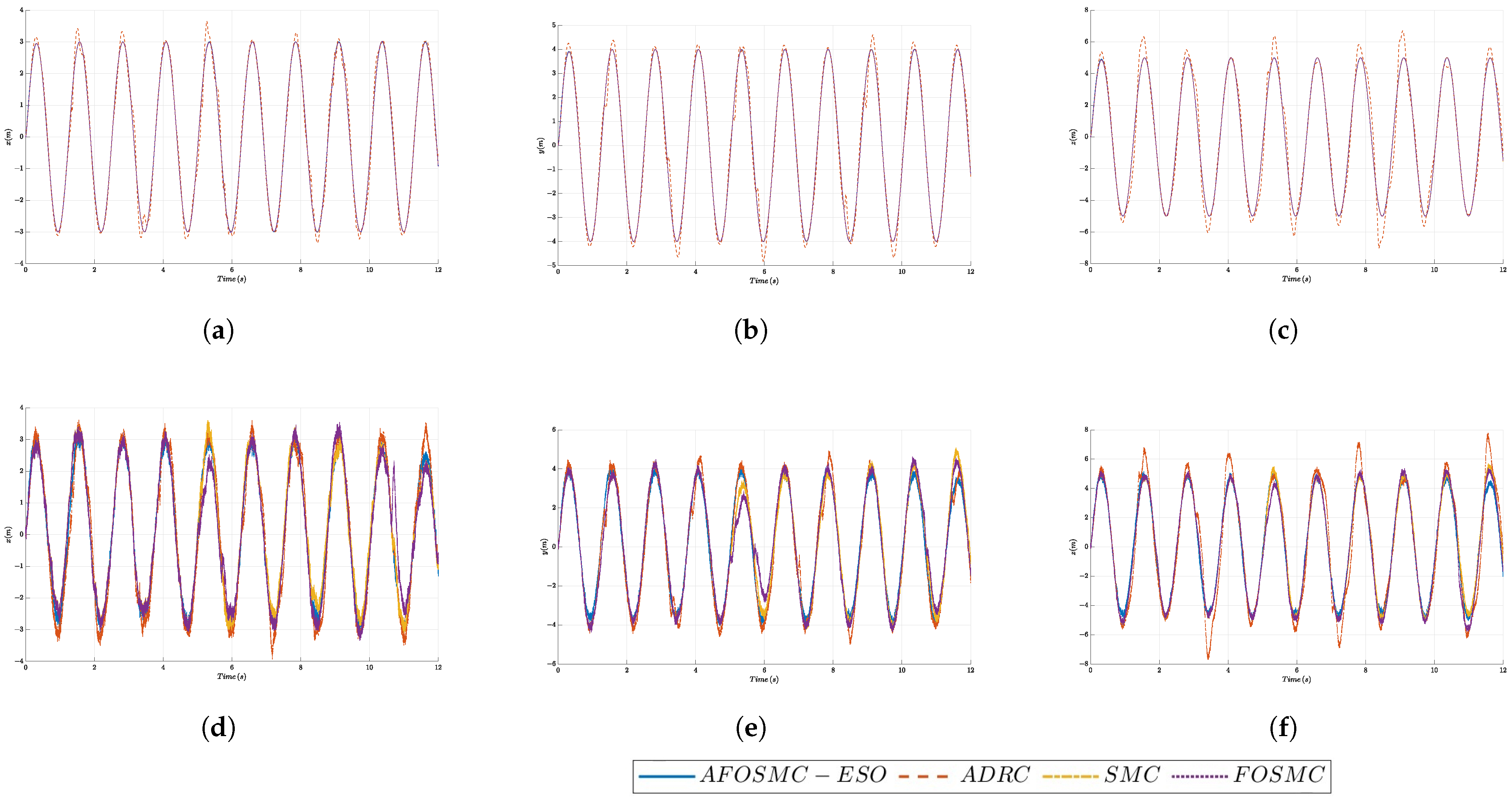
In this subsection, the desired pose is defined as ${\eta }_d=(3sin\left(5t\right),4sin\left(5t\right),5sin\left(5t\right),0^{\circ }$, $0^{\circ },0^{\circ })$. The system responses and those under noisy conditions are shown in Figure 9. The tracking errors under measurement noise are emphasized. In Figure 9d along the x-axis and Figure 9f along the z-axis, AFOSMC-ESO maintains tracking errors within $\pm 0.005\mathrm{m}$ on the x-axis and $\pm 0.007\mathrm{m}$ on the z-axis, and the noise-induced spikes are the smallest among all controllers. This result confirms that the fractional-order sliding surface combined with a smooth reaching law effectively suppresses the amplification of high-frequency noise. Although ADRC exhibits larger error amplitudes, reaching up to $\pm 0.8\mathrm{m}$ on the x-axis, its noise level remains comparable to AFOSMC-ESO, demonstrating strong noise resistance. In contrast, SMC and FOSMC are more sensitive to noise, with evident high-frequency chattering in the error curves caused by the discontinuous sign function in their reaching laws. Compared with other methods, ADRC shows the largest tracking error, whereas AFOSMC-ESO exhibits the smallest error range. The detailed tracking error ranges under sinusoidal motion are summarized in

Table 7. Performance comparison of sinusoidal position tracking with disturbances.

Controller	X-Error (m)	Y-Error (m)	Z-Error (m)
AFOSMC-ESO	$[-1.069,2.438]\times {10}^{-3}$	$[-2.754,3.076]\times {10}^{-3}$	$[-4.261,6.424]\times {10}^{-3}$
ADRC	$[-8.564,7.624]\times {10}^{-1}$	$[-1.403,1.359]$	$[-1.973,2.585]$
FOSMC	$[-2.031,1.988]\times {10}^{-2}$	$[-1.417,1.344]\times {10}^{-2}$	$[-1.320,1.163]\times {10}^{-2}$
SMC	$[-2.062,2.025]\times {10}^{-2}$	$[-1.437,1.369]\times {10}^{-2}$	$[-1.345,1.193]\times {10}^{-2}$

. The RMS values under noisy conditions are listed in Table 6, indicating that AFOSMC-ESO achieves the best noise attenuation performance.

4.4. Circular-Trajectory Tracking with Model Uncertainties

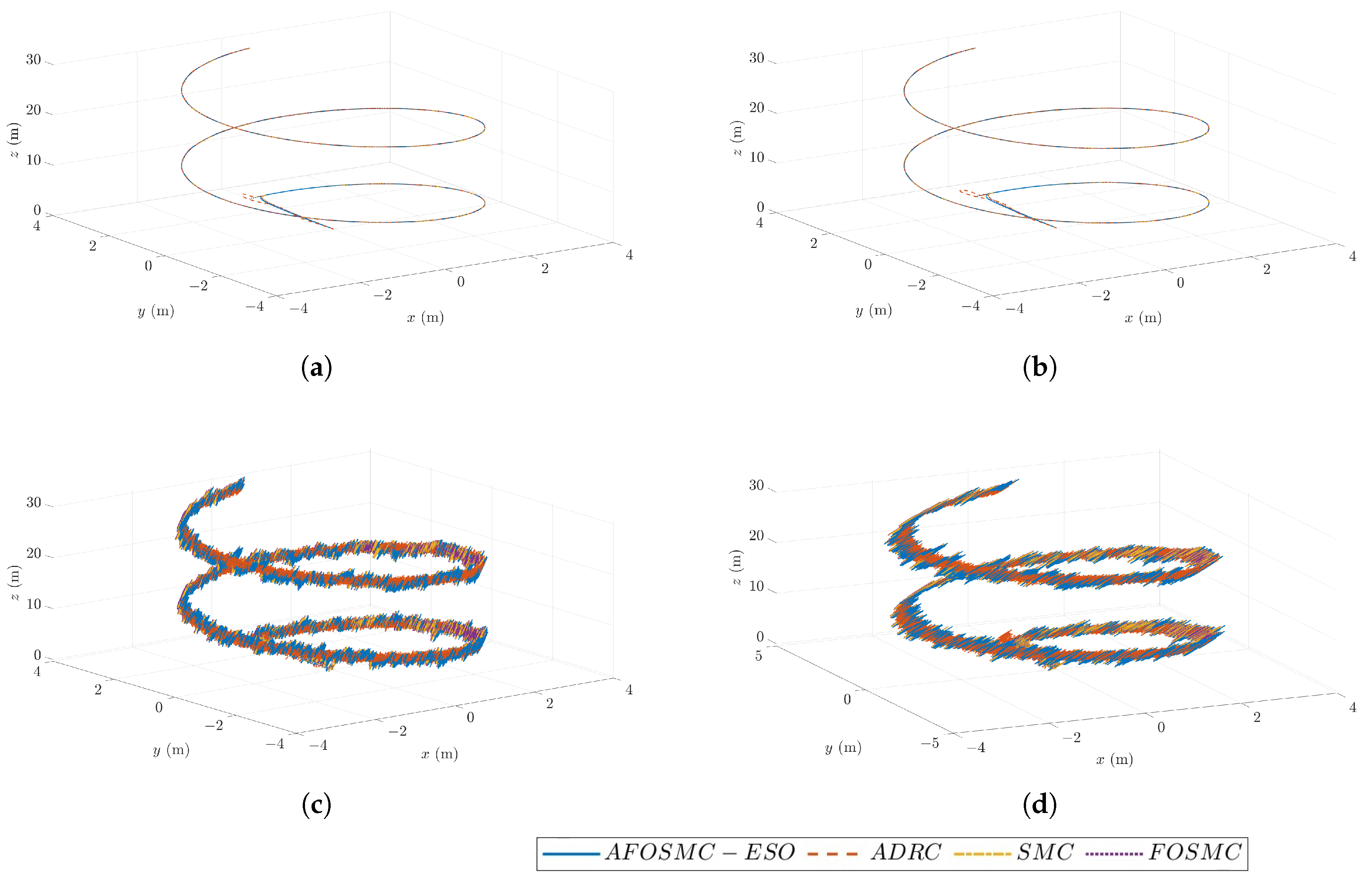
In this subsection, the tracking performance of different control strategies for a circular trajectory is evaluated. The AUV starts from the origin, and the desired pose is defined as ${\eta }_d=\left(3sin\left(0.04\pi t\right),3cos\left(0.04\pi t\right),0.3t,0^{\circ },-{45}^{\circ },{60}^{\circ }\right)$. Moreover, the control performance under model uncertainties is analyzed. It is noted that due to modeling assumptions and simplifications, inherent modeling errors are inevitable. Therefore, this study considers a scenario in which the total inertia, Coriolis effects, hydrodynamic damping, and restoring forces each have 50% uncertainty. The tracking performance under both nominal and uncertain conditions is illustrated in Figure 10. Detailed comparisons are given in

Table 8. Performance comparison of circular-trajectory tracking.

Controller	0% Uncertainty				50% Uncertainty
	ST (s)	X (m)	Y (m)	Z (m)	ST (s)	X (m)	Y (m)	Z (m)
AFOSMC-ESO	0.783	$2.232\times {10}^{-4}$	$8.237\times {10}^{-4}$	$1.393\times {10}^{-4}$	0.657	$4.348\times {10}^{-4}$	$7.908\times {10}^{-2}$	$1.612\times {10}^{-4}$
ADRC	0.336	$2.202\times {10}^{-3}$	$5.701\times {10}^{-2}$	$1.525\times {10}^{-3}$	0.323	$3.249\times {10}^{-3}$	$6.285\times {10}^{-2}$	$2.160\times {10}^{-3}$
FOSMC	0.918	$4.188\times {10}^{-3}$	$1.067\times {10}^{-1}$	$1.137\times {10}^{-2}$	0.688	$3.587\times {10}^{-3}$	$1.019\times {10}^{-1}$	$9.416\times {10}^{-3}$
SMC	0.930	$4.263\times {10}^{-3}$	$1.085\times {10}^{-1}$	$1.158\times {10}^{-2}$	0.695	$3.646\times {10}^{-3}$	$1.034\times {10}^{-1}$	$9.583\times {10}^{-3}$

, while the results under measurement noise are summarized in

Table 9. Performance comparison of circular-trajectory tracking under measurement noise.

Controller	0% Uncertainty			50% Uncertainty
	X (m)	Y (m)	Z (m)	X (m)	Y (m)	Z (m)
AFOSMC-ESO	0.020	0.021	0.020	0.188	0.199	0.187
ADRC	0.103	0.117	0.103	0.120	0.120	0.103
FOSMC	0.190	0.220	0.190	0.172	0.206	0.165
SMC	0.190	0.220	0.190	0.172	0.202	0.164

.

Since the AUV starts from the origin, the initial errors in the X and Z directions are zero. Accordingly, the settling times reported in the tables refer specifically to the Y-direction response. The results demonstrate that even with 50% model uncertainty, all four controllers effectively suppress internal dynamic disturbances without producing significant trajectory-tracking errors. Among them, ADRC achieves the shortest settling time in the Y direction, whereas in terms of control accuracy, the proposed AFOSMC-ESO exhibits superior performance compared with the other algorithms.

4.5. Summary of Simulation Results

Based on the outcomes obtained from the simulations, this subsection presents a detailed analysis and evaluation of the four control strategies.

Table 10. Overall performance comparison of different controllers.

Performance Metric	AFOSMC-ESO	ADRC	SMC	FOSMC
Step-response overshoot	None	Large (17–21%)	Small (0.5%)	Small (0.5%)
Settling time (s)	0.617–0.783	Shortest (0.240–0.336)	0.69–0.93	0.68–0.92
Disturbance rejection	Best (<0.001 m)	Good	Poor	Poor
Robustness	Very strong (50% uncertainty)	Weak	Strong	Strong
Noise attenuation	Good	Best	Good	Good

provides a comparison of their overall performance in terms of step response, disturbance rejection, robustness against model uncertainties, and noise attenuation. The main findings can be summarized as follows:

• In the step-response test, the AFOSMC-ESO can achieve zero overshoot and, during sinusoidal tracking, it exhibits the smallest error amplitude of less than $\pm 7\times {10}^{-3}$ m, which indicates that this controller possesses the highest tracking precision among all strategies examined in the study.
• Under the influence of external disturbances, both AFOSMC-ESO and ADRC are able to maintain position fluctuations within $\pm 0.001$ m; however, the AFOSMC-ESO converges at a faster rate, suggesting that it demonstrates superior disturbance rejection capability compared with other controllers.
• When the system is subjected to 50% model uncertainty, the AFOSMC-ESO remains capable of sustaining stable tracking performance, whereas the ADRC experiences a noticeable degradation in accuracy, indicating that the AFOSMC-ESO provides enhanced robustness with respect to modeling errors.
• In terms of noise attenuation, although the ADRC exhibits the most effective suppression of measurement noise, the AFOSMC-ESO achieves a performance that is comparable to that of the SMC and FOSMC while maintaining greater tracking precision, thereby demonstrating a favorable balance between robustness and accuracy.

In conclusion, AFOSMC-ESO exhibits a balanced performance across response speed, accuracy, robustness, and disturbance rejection in challenging underwater environments with uncertainties. Its overall capability surpasses the other control methods, highlighting its potential for precise AUV trajectory tracking.

5. Conclusions

This work addresses the AUV trajectory-tracking problem in uncertain and disturbed environments by introducing a composite control framework, AFOSMC-ESO, that integrates feedback linearization, an ESO, adaptive regulation, and fractional-order sliding-mode control. Within the framework, feedback linearization neutralizes nonlinear dynamics, the ESO estimates and compensates for total disturbances in real time, and the fractional-order sliding-mode law enhances tracking precision while reducing chattering.

Simulation results from step, sinusoidal, and circular trajectories demonstrate that AFOSMC-ESO achieves zero overshoot, maintains sub-millimeter fluctuations under disturbances, and exhibits the smallest trajectory-tracking errors during periodic motion. Even under severe model uncertainties (50%), AFOSMC-ESO achieves stable tracking with minimal performance degradation, surpassing the other controllers in robustness. Although ADRC provides slightly better noise suppression, AFOSMC-ESO offers a well-balanced performance across accuracy, disturbance rejection, robustness, and noise attenuation, making it highly suitable for precise AUV control in complex underwater conditions.

Future work will focus on validating the proposed strategy through real-world AUV experiments, performing engineering optimizations, integrating AFOSMC-ESO with model predictive control to enhance adaptability in dynamically unknown environments, and extending the framework to multi-AUV cooperative control applications.

References

1. Kotov, D.; Pervukhin, D.; Davardoost, H.; Afanaseva, O. Prospects for the Use of Autonomous Underwater Vehicles (AUV) to Solve the Problems of the Mineral Resources Complex (MRC) of the Russian Federation. J. Marit. Res. 2024, 21, 309–317. [Google Scholar]
2. Xu, H.; Lü, F.; Shi, K.; Zhu, B.; Chen, Z. Research status and development trends of deep-sea long-term resident autonomous underwater vehicle systems. Robot 2023, 45, 720–736. [Google Scholar] [CrossRef]
3. Chen, J.; Xiao, D. Development and prospect of underwater archaeology in China. Sci. Technol. Rev. 2024, 42, 38–47. [Google Scholar] [CrossRef]
4. Lu, G.; Zhang, T.; Li, Z.; Jiang, D.; Lei, M. Development status and key technologies of deep-sea towing autonomous underwater vehicles. Chin. J. Ship Res. 2025, 20, 1–13. [Google Scholar] [CrossRef]
5. Cho, G.R.; Park, D.-G.; Kang, H.; Lee, M.-J.; Li, J.-H. Horizontal Trajectory Tracking of Underactuated AUV using Backstepping Approach. IFAC-PapersOnLine 2019, 52, 174–179. [Google Scholar] [CrossRef]
6. Wang, Y.; Ren, Z.; Shao, X.; Wang, X. Fixed-time cooperative control for multiple surface vessels based on nonsingular fast terminal sliding mode. Control Decis. 2024, 39, 2637–2646. [Google Scholar] [CrossRef]
7. Souissi, S.; Boukattaya, M.; Damak, T.; Nejim, S. Adaptive control for fully-actuated autonomous surface vehicle with uncertain model and unknown ocean currents. Ocean Eng. 2020, 217, 108147. [Google Scholar] [CrossRef]
8. Yan, Z.; Yan, J.; Cai, S.; Yu, Y.; Wu, Y. Robust MPC-based trajectory tracking of autonomous underwater vehicles with model uncertainty. Ocean Eng. 2023, 286, 115617. [Google Scholar] [CrossRef]
9. Li, Y.; Liu, L.; Wang, Y. Optimal equivalent compensation trajectory tracking control for underactuated underwater robots. Control Decis. 2024, 39, 2923–2931. [Google Scholar] [CrossRef]
10. Liu, X.; Sun, B.; Su, Z. Adaptive sliding mode control for AUV based on backstepping and neural networks. Meas. Sci. Technol. 2025, 36, 016215. [Google Scholar] [CrossRef]
11. Li, L.; Cao, Y.; Liang, J.; Zhong, H.; Zhang, H.; Wang, Y. Finite-time adaptive sliding mode tracking control for a quadrotor unmanned aerial vehicle with model uncertainties and external disturbances. Sci. China Technol. Sci. 2026, 69, 1100304. [Google Scholar] [CrossRef]
12. He, L.; Xie, M.; Zhang, Y.; Li, S.; Li, B.; Yuan, Z.; Bai, C. Formation Control of Underactuated AUVs Using a Fractional-Order Sliding Mode Observer. Fractal Fract. 2025, 9, 465. [Google Scholar] [CrossRef]
13. Zhang, H.; Wang, J. Fault-tolerant control of AUV thruster based on adaptive backstepping sliding mode. J. Unmanned Undersea Syst. 2021, 29, 420–427. [Google Scholar] [CrossRef]
14. Zheng, Z.; Ruan, L.; Zhu, M. Output-constrained tracking control of an underactuated autonomous underwater vehicle with uncertainties. Ocean Eng. 2019, 175, 241–250. [Google Scholar] [CrossRef]
15. Qiao, L.; Zhang, W. Trajectory tracking control of AUVs via adaptive fast nonsingular integral terminal sliding-mode control. IEEE Trans. Ind. Inform. 2019, 16, 1248–1258. [Google Scholar] [CrossRef]
16. Thuruthel, T.G.; Ansari, Y.; Falotico, E.; Laschi, C. Control strategies for soft robotic manipulators: A survey. Soft Robot. 2018, 5, 149–163. [Google Scholar] [CrossRef] [PubMed]
17. Relaño, C.; Muñoz, J.; Monje, C.A.; Martínez, S.; González, D. Modeling and control of a soft robotic arm based on a fractional order control approach. Fractal Fract. 2022, 7, 8. [Google Scholar] [CrossRef]
18. Liang, X.; He, G.; Su, T.; Wang, W.; Huang, C.; Zhao, Q.; Hou, Z.-G. Finite-time observer-based variable impedance control of cable-driven continuum manipulators. IEEE Trans. Hum.-Mach. Syst. 2021, 52, 26–40. [Google Scholar] [CrossRef]
19. Shao, X.; Pustina, P.; Stölzle, M.; Sun, G.; De Luca, A.; Wu, L.; Della Santina, C. Model-based control for soft robots with system uncertainties and input saturation. IEEE Trans. Ind. Electron. 2023, 71, 7435–7444. [Google Scholar] [CrossRef]
20. Cao, Y.; Yang, W.; Wang, S.; He, S.; Liu, Z.; Xie, L. Improved trajectory tracking control for a continuum robot using error-driven ADRC with input mapping method. IEEE Trans. Ind. Electron. 2024, 71, 12696–12706. [Google Scholar] [CrossRef]
21. Yu, X.; Feng, Y.; Man, Z. Terminal sliding mode control–an overview. IEEE Open J. Ind. Electron. Soc. 2020, 2, 36–52. [Google Scholar] [CrossRef]
22. Chen, P.; Luo, Y. Analytical fractional-order PID controller design with Bode’s ideal cutoff filter for PMSM speed servo system. IEEE Trans. Ind. Electron. 2022, 70, 1783–1793. [Google Scholar] [CrossRef]
23. Ma, Z.; Liu, Z.; Huang, P.; Kuang, Z. Adaptive fractional-order sliding-mode control for admittance-based telerobotic system with optimized order and force estimation. IEEE Trans. Ind. Electron. 2021, 69, 5165–5174. [Google Scholar] [CrossRef]
24. Fei, J.; Wang, H.; Fang, Y. Novel neural network fractional-order sliding-mode control with application to active power filter. IEEE Trans. Syst. Man. Cybern. Syst. 2021, 52, 3508–3518. [Google Scholar] [CrossRef]
25. Wang, J.; Shao, C.; Chen, Y.-Q. Fractional order sliding mode control via disturbance observer for a class of fractional order systems with mismatched disturbance. Mechatronics 2018, 53, 8–19. [Google Scholar] [CrossRef]
26. Ding, S.; Hou, Q.; Wang, H. Disturbance-observer-based second-order sliding mode controller for speed control of PMSM drives. IEEE Trans. Energy Convers. 2022, 38, 100–110. [Google Scholar] [CrossRef]
27. Han, J. From PID to active disturbance rejection control. IEEE Trans. Ind. Electron. 2009, 56, 900–906. [Google Scholar] [CrossRef]
28. Huang, Y.; Xue, W. Active disturbance rejection control: Methodology and theoretical analysis. ISA Trans. 2014, 53, 963–976. [Google Scholar] [CrossRef]
29. Chen, P.; Gan, H.; Liu, Y.; Luo, Y. Different model-based ADRCs satisfying performance independent control for PMSM speed servo system. IEEE Trans. Ind. Electron. 2024, 72, 2012–2023. [Google Scholar] [CrossRef]
30. Al-Dhaifallah, M.; Saif, A.-W.A.; Elferik, S.; Elkhider, S.M.; Aldean, A.S. Combining Sliding Mode and Fractional-Order Theory for Maximum Power Point Tracking Enhancement of Variable-Speed Wind Energy Conversion. Fractal Fract. 2024, 8, 447. [Google Scholar] [CrossRef]
31. Dang, Z. Research on Motion Attitude Control Method of Underwater Vehicles; Jiangxi University of Science and Technology: Jiangxi, China, 2023; p. 86. Available online: https://link.cnki.net/doi/10.27176/d.cnki.gnfyc.2023.000557 (accessed on 27 May 2026).
32. Wang, Y.; Hou, Y.; Lai, Z.; Cao, L.; Hong, W.; Wu, D. An adaptive PID controller for path following of autonomous underwater vehicle based on Soft Actor–Critic. Ocean Eng. 2024, 307, 118171. [Google Scholar] [CrossRef]
Figure 1. Inertial and body-fixed coordinate frames.
Fractalfract 10 00398 g001
Figure 2. Control block diagram of the system.
Fractalfract 10 00398 g002
Figure 3. Noise magnitude.
Fractalfract 10 00398 g003
Figure 4. Comparison between the approximated Bode plot and the true Bode plot
Fractalfract 10 00398 g004
Figure 5. Tracking performance comparison of the Levant differentiator: (a) x-axis tracking error, (b) y-axis tracking error, (c) z-axis tracking error, (d) roll tracking error, (e) pitch tracking error, and (f) yaw tracking error.
Fractalfract 10 00398 g005
Figure 6. Step position tracking response: (a) x-axis within 0–2 s, (b) y-axis within 0–2 s, (c) z-axis within 0–2 s, (d) x-axis within 4–12 s, (e) y-axis within 4–12 s, (f) z-axis within 4–12 s, (g) x-axis under measurement noise, (h) y-axis under measurement noise, and (i) z-axis under measurement noise.
Fractalfract 10 00398 g006
Figure 7. Step position control forces along (a) x-axis, (b) y-axis, and (c) z-axis within 0–2 s.
Fractalfract 10 00398 g007
Figure 8. Step position tracking response under external disturbances applied to the control force: (a) x-axis within 0–3 s, (b) y-axis within 0–3 s, and (c) z-axis within 0–3 s.
Fractalfract 10 00398 g008
Figure 9. Sinusoidal position tracking responses: (a) comparison of controller performance along the x-axis, (b) along the y-axis, (c) along the z-axis, (d) x-axis under measurement noise, (e) y-axis under measurement noise, and (f) z-axis under measurement noise.
Fractalfract 10 00398 g009
Figure 10. Circular-trajectory tracking: (a) performance comparison of different controllers under the nominal model, (b) performance comparison under 50% model uncertainty, (c) performance comparison under the nominal model with measurement noise, and (d) performance comparison under 50% model uncertainty with measurement noise.
Fractalfract 10 00398 g010