Unlocking Multifractal and Long-Memory Dynamics in Cryptocurrency Markets: A Fractional Attention-Driven LSTM–N-BEATS Framework for Optimal Investment Under Dynamic Risk

Abstract

Cryptocurrency markets exhibit persistent temporal dependence and multifractal scaling behavior, yet these properties remain only partially incorporated into existing deep learning architectures. This study proposes the Fractional Attention-Driven LSTM–N-BEATS (FA-LSTM-NBEATS) framework, integrating Grünwald–Letnikov fractional memory operators, adaptive attention, interpretable N-BEATS decomposition, and an asymmetric loss function within a unified forecasting and risk estimation model. The framework is evaluated using daily BTC, ETH, and BNB data from 2018 to 2025 through hierarchical ablation analysis, walk-forward validation, Diebold–Mariano testing, residual diagnostics, and Fractional Value-at-Risk (VaR) evaluation. Results indicate persistent scaling behavior with Hurst exponents above 0.76 and multifractal spectrum widths of $\mathrm{\Delta }\alpha \approx 0.51–0.54$. FA-LSTM-NBEATS achieves the strongest relative forecasting performance for BNB, with the lowest RMSE (0.02789) and MAE (0.01950) among all evaluated models. The learned fractional parameter $\left(\alpha ≈0.6106\right)$ remains stable across assets, suggesting convergence toward a persistent memory regime. In addition, Fractional VaR produces coverage ratios closer to unity than Historical and LSTM-based benchmarks under high-volatility conditions.

1. Introduction

Cryptocurrency markets have emerged as an increasingly relevant asset class in the global financial landscape. Since the emergence of Bitcoin in 2009, the crypto ecosystem has grown to encompass thousands of digital assets with substantial market capitalization. Unlike conventional assets such as stocks or bonds, cryptocurrency markets operate continuously, 24 h a day and 7 days a week. There is no centralized regulatory authority governing their movements. Extreme volatility, non-normal return distributions, and strong nonlinearity are among their defining characteristics [1,2]. Transaction volumes have grown steadily, and institutional investor participation has increased. These conditions underscore the urgency of developing a deeper understanding of market dynamics. As a result, predicting cryptocurrency prices is one of the most significant challenges in modern computational finance. This challenge drives the need for predictive models that more faithfully represent true market behavior.

A growing body of literature documents statistical characteristics that distinguish cryptocurrency markets from conventional financial assets. One frequently reported finding is the presence of persistent multifractal properties and long memory in cryptocurrency price series [3,4,5]. Multifractality shows that cryptocurrency markets have complex, heterogeneous scaling across time scales. This means that price dynamics at the minute, hourly, and daily levels do not follow simple or homogeneous patterns. Long memory means current prices are influenced by distant past values, more so than conventional short-memory models can capture. In theory, cryptocurrency markets do not conform to the Efficient Market Hypothesis, even in its weakest form [4]. This long-range temporal dependence holds substantial predictive information. Models designed to use this structure could potentially exploit it.

Studies focusing on multifractal analysis of cryptocurrency markets have made important contributions to understanding the sources and characteristics of this phenomenon. Drożdż et al. [5] conducted a comprehensive analysis of digital currency markets using MFDFA and MF-CCA, finding that long-range correlations are a more dominant source of multifractality than heavy-tailed distributions. Ali et al. [6] extended this understanding by analyzing multifractal dynamics specifically in price jumps using 5 min intraday data, confirming high persistence across all assets examined. Despite the analytical richness of these findings, both studies are entirely descriptive. No attempt was made to translate these structural findings into an operationalizable forecasting framework. This constitutes one of the most fundamental gaps that remains open in the literature.

On the other side, the deep learning community has produced a wide range of predictive models for cryptocurrency prices with increasingly high accuracy. Recurrent Neural Network (RNN) architectures, particularly Long Short-Term Memory (LSTM) and its variants, have become the dominant choice due to their ability to capture sequential patterns in time series data [7,8]. Furthermore, recent advancements have demonstrated that LSTM networks are not only effective for standalone economic indicators but also highly capable of processing and predicting time series data derived from multi-dimensional hyperchaotic systems characterized by extreme volatility and structural complexity [9]. This underscores the model’s fundamental suitability for complex, nonlinear sequences before extending them into fractional-order domains.

Seabe et al. [10] demonstrated that Bi-LSTM can predict the prices of Bitcoin (BTC), Litecoin, and Ethereum (ETH) with competitive error rates. Badar et al. [11] achieved an R² of 0.99 for Bitcoin using a hybrid architecture combining a Variational Autoencoder, Convolutional Neural Network (CNN), and LSTM. Jin & Li [12] showed that combining Variational Mode Decomposition (VMD) with attention GRU and LSTM yields a Bitcoin MAPE of approximately 0.394%. Asmat and Maiyama [13] demonstrated the superiority of N-BEATS over LSTM and linear regression for hourly Bitcoin price prediction. Lee [14] integrated attention mechanisms with technical indicators for Bitcoin trend prediction, achieving classification accuracy of approximately 71–73%. While these advances reflect genuine progress in the predictive capacity of deep learning models for cryptocurrency markets, they all share a common structural limitation: none explicitly encode long memory or multifractality into their architectural design [2,15]. This limitation is critical because, as established in contemporary engineering and cryptographic studies, while artificial neural networks (ANNs) excel at capturing the localized complex dynamics of underlying chaotic systems [16], traditional integer-order structures inherently struggle to parameterize the long-range temporal persistence embedded in historical sequences.

To address this limitation, fractional calculus offers a mathematically relevant framework. Unlike integer-order differential operators, fractional operators are inherently capable of representing non-local memory and long-range dependence, which are defining features of long-memory systems [4,17]. David et al. [4] empirically demonstrated that ARFIMA, which is grounded in fractional integration, produces smaller residuals than standard ARIMA on cryptocurrency data. Ez-zaiym et al. [17] integrated fractional derivative-based optimizers into LSTM and reported improved accuracy on financial time series, though only for stock data with moderate volatility. Bildirici et al. [18] combined Lie group algebra with LSTM and showed that the resulting model outperformed ARFIMA on Bitcoin return data spanning 2010 to 2023. Collectively, these studies indicate that incorporating fractional components into predictive models holds genuine potential. However, their application within hybrid deep learning architectures specifically designed to capture the multifractal nature of cryptocurrency markets remains very limited.

Beyond prediction, risk management constitutes an essential component of rational investment decision-making. Subramoney et al. [19] showed that Value-at-Risk (VaR) models incorporating long-memory volatility and heavy-tailed distributions can provide more reliable risk estimates for cryptocurrency assets than conventional approaches. Similarly, Bui et al. [3] identified regime-dependent long-range correlations in cryptocurrency markets using a multi-scale DFA framework, highlighting the relevance of persistence structures for portfolio allocation and volatility management. Collectively, these findings indicate that long-memory characteristics are relevant not only for forecasting purposes but also for improving downside risk estimation under highly volatile market conditions. Nevertheless, most existing deep learning frameworks continue to treat forecasting and risk estimation as separate tasks, with limited integration between predictive modeling and dynamic risk management components.

To address these limitations, this study proposes the Fractional Attention-Driven LSTM–N-BEATS (FA-LSTM-NBEATS) framework, which integrates long-memory representation, multiscale feature extraction, and risk-aware forecasting within a unified architecture. The proposed framework incorporates fractional-order operators into LSTM layers to model power-law memory behavior, an adaptive attention mechanism in the frequency domain to capture heterogeneous temporal dynamics, and an interpretable N-BEATS decoder for structured trend–cycle decomposition. In addition, a Fractional VaR estimation component is incorporated to support dynamic risk assessment in cryptocurrency investment settings. Through this integrated design, the framework aims to provide a representation that is more closely aligned with the multifractal and long-memory characteristics observed in cryptocurrency markets, while simultaneously evaluating the implications for forecasting performance and risk estimation.

2. Related Work

Research on cryptocurrency forecasting increasingly emphasizes the importance of multifractality, long-memory persistence, and nonlinear volatility structures in digital asset markets. Various studies have shown that cryptocurrency return series exhibit statistical characteristics significantly different from those of conventional financial assets, particularly heavy-tailed volatility, regime-dependent persistence, and heterogeneous scaling behavior. Drożdż et al. [5] conducted a comprehensive multifractal investigation using MFDFA, MF-CCA, a reshuffling procedure, and q-Gaussian filtering on BTC, ETH, DEX tokens, and NFT assets. The results of this study showed that long-term temporal correlation is the main source of multifractality, while heavy-tail distribution mainly amplifies the observed complexity. Ali et al. [6] also analyzed cryptocurrency jump dynamics using intraday data and found that multifractal persistence is not limited to continuous return dynamics but also extends to discontinuous price jumps. David et al. [4] further demonstrated, using DFA, Hurst exponent analysis, and ARFIMA modeling, that Bitcoin exhibits significant long-memory behavior and that the fractional integration approach outperforms conventional ARIMA models in capturing the persistent structure of cryptocurrency. Additional evidence is provided by Bui et al. [3], who identified long-range correlations that change with market regimes using multi-scale DFA, while Subramoney et al. [19] demonstrated that long-memory volatility models can improve VaR estimates under extreme conditions in the cryptocurrency market. Overall, these studies provide a strong empirical basis for demonstrating that cryptocurrency markets exhibit persistent, multifractal temporal structures relevant to both forecasting and risk estimation.

In parallel with the development of fractal-based market analysis, deep learning architectures for cryptocurrency forecasting have also rapidly evolved. Recurrent neural network models, particularly variants of LSTM and GRU, have become the most widely used approaches in the literature. Seabe et al. [10] compared LSTM, GRU, and Bi-LSTM architectures for BTC, LTC, and ETH price prediction, and found that Bi-LSTM consistently produced the best forecasting performance. Lee [14] integrated an attention mechanism into an LSTM and GRU framework for Bitcoin trend classification using various technical indicators and demonstrated that attention improved sequential learning representations. More complex hybrid architectures have also been developed. Badar et al. [11] proposed a VAE–CNN–LSTM framework combined with SHAP-based explainable AI, while Jin and Li [11] integrated Variational Mode Decomposition (VMD) with attention-based GRU and LSTM for BTC and ETH forecasting. Additionally, Asmat and Maiyama [13] demonstrated that the N-BEATS architecture has strong forecasting capabilities through interpretable basis-expansion decomposition. Although these approaches yield competitive predictive performance, most existing deep learning models still do not explicitly incorporate multifractal structures, long-range persistence, or fractional-order dynamics into their architectures.

In recent years, several studies have begun exploring the integration of fractional calculus into predictive financial modeling. Ez-zaiym et al. [17] introduced a fractional-derivative-based optimizer into the LSTM training process and reported improved forecasting performance for stocks with moderate volatility. Bildirici et al. [18] developed a more mathematically complex framework combining the SO(3) Lie group algebra and an LSTM architecture for Bitcoin return prediction, demonstrating that mathematical structures capable of representing persistence and chaotic dynamics can improve predictive performance compared to conventional statistical baselines. However, these studies are still limited to optimizer-level modifications or very specific mathematical formulations with limited generalizability. In addition, integrating fractional-order memory, an adaptive attention mechanism, an interpretable decomposition structure, and dynamic risk estimation within a single forecasting framework remains relatively rare.

Based on this gap, this study proposes the Fractional Attention-Driven LSTM–N-BEATS (FA-LSTM-NBEATS) framework to explore the integration of fractional-order memory, adaptive attention mechanism, and interpretable decomposition in cryptocurrency forecasting. Fractional-order operators are integrated into a recurrent structure to model power-law memory and long-term persistence, as indicated by the Hurst exponent and multifractal analysis. Furthermore, the N-BEATS decoder is used to separate trend and cycle components, enabling cryptocurrency return dynamics to be represented in a more structured and interpretable manner. This study also integrates Fractional VaR estimation to evaluate the framework’s implications for risk estimation under persistent, volatile, and non-stationary conditions in the cryptocurrency market.

3. Materials and Methods

3.1. Dataset Description and Feature Construction

This study utilizes daily historical cryptocurrency data sourced directly from yfinance, recognized as the largest centralized digital asset exchange in terms of trading volume. Relying on a single exchange ensures consistency in pricing dynamics, liquidity structure, and execution mechanisms, thereby mitigating distortions that commonly arise from aggregating multi-exchange datasets [19]. This consistency is particularly important given the fragmented and often divergent pricing behavior across cryptocurrency trading venues.

The empirical analysis focuses on three major digital assets: BTC, ETH, and Binance Coin (BNB). These assets represent the core of the cryptocurrency ecosystem while capturing distinct functional roles. BTC operates as a primary store of value and market sentiment benchmark, ETH serves as the leading programmable platform for smart contracts and decentralized finance, and BNB functions as an exchange-native utility token [6,10]. This selection ensures both diversity and structural coherence for cross-asset comparison.

The observation period spans from 1 January 2018 to 31 December 2025, resulting in 2922 daily observations for each asset after preprocessing. This period covers multiple major market regimes, including the post-2017 correction phase, the COVID-19 liquidity shock in 2020, the 2020–2021 bullish expansion, the market disruptions associated with the LUNA/Terra and FTX collapses in 2022, and the subsequent recovery phase through 2025 [19,20]. Such heterogeneous market conditions provide a suitable environment for evaluating forecasting robustness under varying volatility and persistence regimes [21].

The forecasting task is formulated as one-step-ahead return prediction using a rolling window framework. Specifically, the model leverages the previous 20 observations to estimate the return at the next time step. This approach preserves strict temporal causality, prevents information leakage, and aligns with realistic investment horizons [10,17]. To represent market dynamics, the raw price data are transformed into derived features. The logarithmic return is defined as:

$$R_t=\ln \left({\displaystyle \frac{P_t}{P_{t-1}}}\right).$$

(1)

In this formulation, $R_t$ represents the logarithmic return at time $t$, which measures the relative price change between two consecutive periods in a continuous compounding framework. The variable $P_t$ denotes the closing price at time $t$, while $P_{t-1}$ corresponds to the closing price at the immediately preceding time step. The natural logarithm function $\mathrm{l}\mathrm{n}(·)$ is applied to stabilize variance and convert multiplicative price changes into an additive form, thereby improving statistical tractability and comparability across time [12,22].

To capture extreme market fluctuations, a binary indicator variable is introduced as follows:

$$I_{\mathrm{Extreme},t}=\left\{\begin{array}{cc}1,& \mathrm{if} \mid R_t\mid >k\sigma \\ 0,& \mathrm{otherwise}\end{array}\right.,$$

(2)

Here, $I_{\mathrm{Extreme},t}$ identifies whether an extreme return occurs at time $t$, based on the comparison between the absolute return magnitude $\mid R_t\mid$ and a volatility-adjusted threshold $k\sigma$, where $\sigma$ denotes the standard deviation of returns and $k$ controls the sensitivity level. The final input representation consists of normalized OHLC prices, logarithmic returns, and the extreme event indicator, forming a six-dimensional feature space. The dataset is split chronologically into training (70%), validation (15%), and testing (15%) sets, ensuring that evaluation is strictly conducted on unseen future data. All computations and model training were performed using Google Colaboratory (Google LLC, Mountain View, CA, USA). The proposed FA-LSTM-NBEATS framework was implemented in Python (Python Software Foundation, Wilmington, DE, USA, https://www.python.org/ (accessed on 27 May 2026)) using PyTorch (Meta Platforms, Inc., Menlo Park, CA, USA, https://pytorch.org/ (accessed on 27 May 2026)). Data preprocessing and numerical computations were conducted using pandas, NumPy, and SciPy, while statistical analyses utilized Statsmodels and scikit-learn (INRIA, Paris, France). Visualization was performed using Matplotlib (https://matplotlib.org/ (accessed on 27 May 2026)). GPU acceleration was enabled through CUDA (NVIDIA Corporation, Santa Clara, CA, USA).

3.2. Long-Memory Analysis via Hurst Exponent

Before introducing the proposed deep learning framework, it is important to examine whether the cryptocurrency return series exhibits scaling behavior consistent with long-range temporal dependence from a statistical physics perspective. The presence of such dependence would imply that past market dynamics continue to influence future behavior over extended horizons, thereby challenging the short-memory assumptions commonly embedded in conventional Markovian forecasting models [17,23].

To investigate this property, the classical Rescaled Range (R/S) method is employed to estimate the Hurst exponent for each asset. For a stochastic time series, the rescaled range statistic follows the power-law relationship as:

$$\left(R/S{)}_n\sim c·n^H\right.,$$

(3)

where $H$ denotes the Hurst exponent and is estimated through ordinary least squares (OLS) regression in log–log space. The interpretation of $H$ is well established in long-memory analysis: $H=0.5$ corresponds to an uncorrelated random walk process, $H>0.5$ indicates persistent dependence, and $H<0.5$ reflects anti-persistent or mean-reverting dynamics.

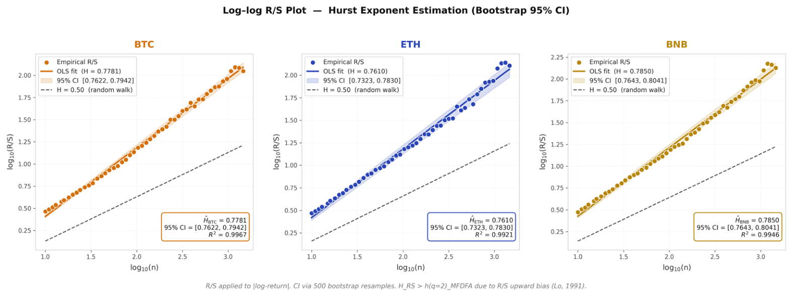
Figure 1 presents the log–log R/S scaling behavior for BTC, ETH, and BNB daily log-return series over the 2018–2025 observation period. The fitted scaling relationships were estimated over the selected scaling range using OLS regression, while uncertainty was evaluated through 500 bootstrap resamples to obtain 95% confidence intervals. The estimated Hurst exponents are:

$$H_{BTC}=0.7781,H_{ETH}=0.7610,H_{BNB}=0.7850.$$

All estimated values remain consistently above the random walk benchmark $\left(H=0.5\right)$, indicating scaling behavior consistent with persistent temporal dependence. Among the three assets, BNB exhibits the highest persistence level, while ETH shows slightly lower scaling intensity. BTC remains within a comparable range, suggesting that long-memory behavior may represent a broader structural characteristic of cryptocurrency markets rather than an isolated asset-specific phenomenon.

It should be noted, however, that the R/S-based Hurst estimates reported here are systematically higher than the generalized Hurst exponents $h(q=2)$ obtained later through MF-DFA analysis in Section 3.3. This discrepancy is consistent with the known upward bias of classical R/S estimators under finite-sample conditions and heteroskedastic volatility regimes [24]. Therefore, the R/S analysis in this study is interpreted primarily as qualitative evidence of persistence rather than as an exact scaling-equivalence measure relative to MF-DFA.

From a modeling perspective, the condition $H>0.5$ suggests that historical return sequences retain non-negligible influence over future market dynamics across extended horizons. Such behavior may not be fully captured by exponentially decaying memory structures embedded in standard LSTM architectures. Consequently, these findings provide a preliminary empirical motivation for exploring fractional-order memory operators within the proposed FA-LSTM-NBEATS framework, as fractional dynamics are theoretically compatible with power-law memory decay and persistent temporal dependence [23,24].

3.3. Multifractal Characterization via Singularity Spectrum Analysis

Having established scaling behavior consistent with long-range dependence, the analysis is further extended to investigate the heterogeneity of volatility dynamics across multiple temporal scales using Multifractal Detrended Fluctuation Analysis (MF-DFA), which enables the characterization of scale-dependent persistence through the generalized Hurst exponent $h\left(q\right)$ and the singularity spectrum $f\left(\alpha \right)$ [15,20,25]. The degree of multifractality is quantified by the width of the singularity spectrum, defined as:

$$\mathrm{\Delta }\alpha ={\alpha }_{\mathrm{m}\mathrm{a}\mathrm{x}}-{\alpha }_{\mathrm{m}\mathrm{i}\mathrm{n}},$$

(4)

where $\mathrm{\Delta }\alpha$ measures the range of local Hölder exponents, with larger values indicating broader variability in local scaling behavior and greater heterogeneity in volatility dynamics [20,26]. In this context, $\alpha$ denotes the local Hölder exponent associated with the multifractal spectrum and should not be confused with the learnable fractional-order parameter used later in the proposed FA-LSTM-NBEATS architecture. In multifractal systems, the singularity spectrum $f\left(\alpha \right)$ is mathematically related to the generalized dimension spectrum through the Legendre transformation of the mass exponent function $\tau \left(q\right)$. A broader singularity spectrum generally corresponds to stronger variability in generalized dimensions across scaling orders, indicating higher heterogeneity in temporal organization and scale-dependent persistence. Conversely, when the spectrum width approaches zero, the system tends toward monofractal behavior characterized by more uniform scaling properties across temporal scales.

In multifractal systems, a singularity spectrum width approaching zero indicates near-monofractal behavior characterized by relatively homogeneous scaling properties across temporal scales. Conversely, broader singularity spectra indicate stronger heterogeneity in local scaling behavior and more complex temporal organization. The moderate spectrum widths obtained in the present study therefore suggest the presence of persistent multifractal volatility structures across all analyzed cryptocurrency assets. These findings remain broadly consistent with previous studies of cryptocurrency MF-DFA. For example, Drożdż et al. [5] demonstrated that cryptocurrency markets exhibit broad multifractal spectra driven primarily by nonlinear temporal correlations rather than heavy-tailed distributions alone. However, compared with high-frequency intraday studies where the number of observations often exceeds 20,000, the present estimates derived from 2922 daily observations should be interpreted more cautiously as indicative evidence of heterogeneous scaling rather than definitive quantification of market complexity.

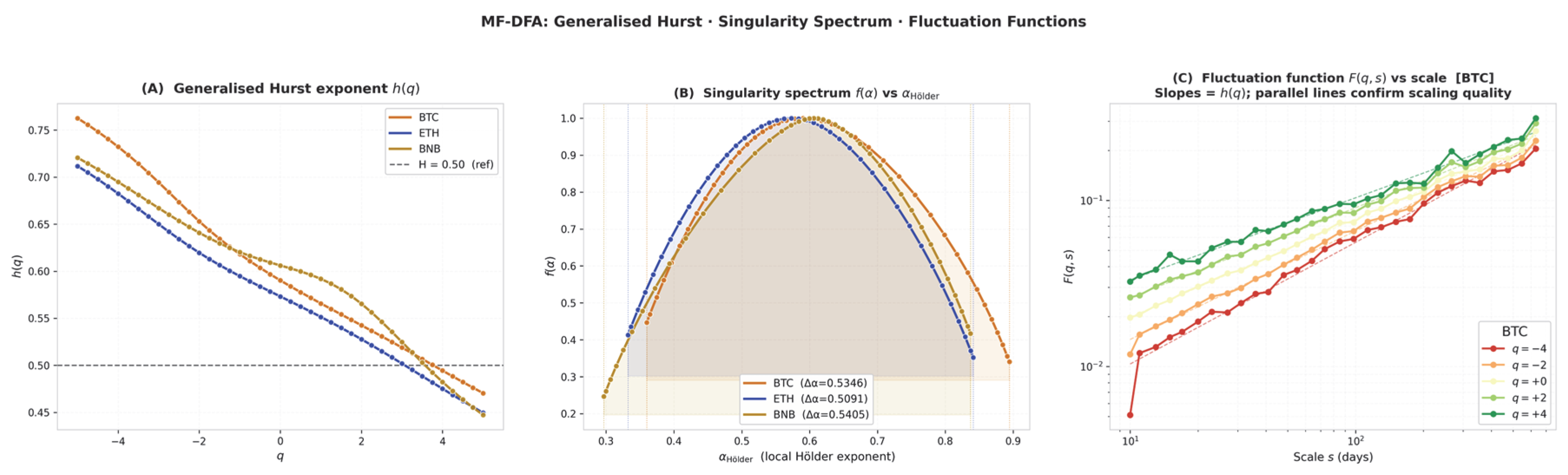
As illustrated in Figure 2, all analyzed assets exhibit nonlinear $h\left(q\right)$ profiles across $q\in [-\mathrm{5,5}]$, indicating deviation from monofractal scaling and suggesting the presence of scale-dependent persistence structures [5,6]. In particular, the estimated values of $h(q=2)$ remain moderately above the random walk benchmark, although systematically lower than the R/S-based Hurst exponents reported in Section 3.2, which is consistent with the known upward bias of classical R/S estimators under finite-sample and heteroskedastic conditions [4,26]. The corresponding singularity spectra $f\left(\alpha \right)$ exhibit smooth concave shapes consistent with multifractal scaling behavior [5,18]. The estimated spectrum widths are $\mathrm{\Delta }{\alpha }_{BTC}=0.5346$, $\mathrm{\Delta }{\alpha }_{ETH}=0.5091$, and $\mathrm{\Delta }{\alpha }_{BNB}=0.5405$, with BNB exhibiting the widest spectrum, followed closely by BTC, while ETH shows a slightly narrower distribution of local scaling exponents. These differences suggest moderate variation in multi-scale heterogeneity across assets, potentially reflecting differences in liquidity structure, trading intensity, and market microstructure dynamics [3,6].

The discrepancy between the relatively high R/S-based Hurst estimates and the lower generalized Hurst exponents obtained via MF-DFA is consistent with the known methodological differences between classical rescaled-range analysis and detrended fluctuation-based scaling estimators. Classical R/S estimators are known to exhibit upward bias under finite-sample conditions, volatility clustering, and heteroskedastic nonstationary environments, whereas MF-DFA provides a more conservative and robust characterization of scale-dependent persistence under multifractal conditions. Consequently, the two scaling measures should not be interpreted as numerically interchangeable, despite both reflecting evidence of persistent temporal dependence.

To further assess the reliability of the MF-DFA procedure, the fluctuation functions $F_q\left(s\right)$ presented in Figure 2 exhibit approximately linear log–log relationships across the analyzed scale range, indicating acceptable scaling consistency within the selected temporal windows [20,25]. Nevertheless, the estimated multifractal spectrum widths obtained from daily observations should be interpreted cautiously, particularly given the relatively small sample size compared with those in high-frequency multifractal studies commonly used in financial markets [5,26]. Therefore, the present findings are interpreted as evidence of multifractal scaling behavior rather than as a definitive quantification of market complexity. The estimated spectrum widths obtained in this study also remain higher than those commonly reported for traditional financial markets, where indices such as the Dow Jones Industrial Average generally exhibit lower degrees of multifractality [26,27]. This observation is consistent with the highly nonlinear, volatile, and non-stationary characteristics widely associated with cryptocurrency markets [3,5]. From a modeling perspective, these results suggest that cryptocurrency volatility dynamics contain heterogeneous temporal structures that may not be fully represented by architectures relying solely on exponentially decaying memory mechanisms, thereby motivating the exploration of fractional-order memory representations whose power-law decay structure is theoretically more compatible with persistent and multi-scale temporal dependence [17,23,24].

3.4. Proposed Framework: Fractional Attention-Driven LSTM–N-BEATS

3.4.1. Grünwald Letnikov Fractional Calculus Foundations

The proposed architecture is based on fractional-order calculus, which generalizes classical differentiation to non-integer orders and provides a natural mathematical framework for representing non-local and history-dependent dynamic processes. This formulation is well suited for modeling the long-memory and multifractal structures observed in financial time series [4,26,27]. The rapid expansion of machine learning applications in finance, comprehensively reviewed by Nazareth et al. [28], Ozbayoglu et al. [29] and Mienye et al. [30], further highlights the inadequacy of conventional integer-order dynamic assumptions to capture the complex temporal dependencies inherent in financial markets. Furthermore, recent studies confirm that fractional-order operators improve neural network performance by enhancing gradient stability and enabling adaptive memory mechanisms, as they explicitly incorporate historical dependencies into the learning process [31]. The Grünwald–Letnikov (GL) formulation is adopted due to its simplicity for discrete-time algorithm implementation.

For a univariate time series $x_t$, the $\alpha$-order GL fractional derivative is expressed as:

$${}^{GL}D^{\alpha }{x}_t=\underset{h\to 0}{\mathrm{l}\mathrm{i}\mathrm{m}}{h}^{-\alpha }{\displaystyle \sum _{j=0}^{\mathrm{\infty }}}(-1{)}^j{\displaystyle \frac{\Gamma (\alpha +1)}{\Gamma (j+1)\hspace{0.17em}\Gamma (\alpha -j+1)}}\hspace{0.17em}{x}_{t-jh},$$

(5)

where ${}^{GL}D^{\alpha }{x}_t$ is the GL fractional derivative of order $\alpha$ of the time series $x_t$, $\alpha$ is the fractional differentiation order, a learnable scalar satisfying $0<\alpha <1$, $h$ is the sampling interval between time points, $j$ is the summation index representing the $j$-th historical lag; $\Gamma (·)$ is the Gamma function, the continuous generalization of the factorial, and (−1)^j is an alternating sign factor characteristic of fractional operators.

Setting $h=1$ and introducing a finite truncation window $W$ to render the operator computationally tractable, the discretized GL approximation becomes:

$$D^{\alpha }{x}_t\approx {\displaystyle \sum _{j=1}^W}{c}_j\left(\alpha \right)\hspace{0.17em}{x}_{t-j},$$

(6)

where $W$ is the truncation window specifying the number of historical steps considered, and $c_j\left(\alpha \right)$ are the GL weighting coefficients for lag $j$ at fractional order $\alpha$, computed through the recurrence:

$$c_j\left(\alpha \right)={\displaystyle \frac{\Gamma \left(j-\alpha \right)}{\Gamma \left(j+1\right)\hspace{0.17em}\Gamma \left(-\alpha \right)}}.$$

(7)

The critical property distinguishing this operator is the asymptotic behavior of $c_j\left(\alpha \right)$: as $j\to \mathrm{\infty }$, $c_j\left(\alpha \right)\sim j^{-(\alpha +1)}$, yielding a power-law decay rather than exponential attenuation. This decay profile is structurally consistent with the empirically observed Hurst exponent values $H\in [0.76,0.79]$, as both reflect slowly attenuating dependence on historical states [4,6]. The parameter $\alpha$ is treated as a learnable scalar updated during backpropagation. It should be emphasized that the fractional-order parameter $\alpha$ used in the Grünwald–Letnikov operator is fundamentally different from the singularity-spectrum variable $\alpha$ in MF-DFA analysis presented in Section 3.3. In the MF-DFA framework, $\alpha$ denotes the local Hölder exponent characterizing multifractal scaling behavior, whereas in the proposed architecture, $\alpha$ represents a learnable fractional differentiation order controlling the strength of power-law memory within the neural network. Therefore, the two quantities are conceptually distinct and are not directly interchangeable, although both are related to scale-dependent temporal dynamics.

3.4.2. Fractional LSTM Encoder with Power-Law Memory

In conventional LSTM architectures, cell states evolve through a combination of gates that incorporate past information and new candidates, resulting in exponential memory decay. While effective in addressing vanishing gradients, this mechanism is poorly suited to power-law temporal dependencies in financial time series [7,15,32].

This limitation was highlighted by Kim et al. [33], and supported by Mienye et al. [30] and Bustos & Pomares-Quimbaya [34], who showed that models without explicit long memory tend to underperform in markets with persistent autocorrelation. In contrast, fractional-order dynamics have been shown to improve the ability to capture long-term dependencies and stability through smoother gradient propagation [23].

To address this, the fractional GL operator is embedded directly into the cell state propagation equation:

$$C_t^F=f_t\odot {\displaystyle \sum _{j=1}^W}{c}_j\left({\alpha }_1\right)\hspace{0.17em}{C}_{t-j}^F+i_t\odot {\tilde{C}}_t^F,$$

(8)

where $C_t^F$ is the fractional LSTM cell state at time $t$, $C_{t-j}^F$ is the fractional cell state $j$ time steps prior to $t$, $f_t$ is the forget gate at time $t$, a vector with values in $\left[0,1\right]$ computed via sigmoid activation, $i_t$ is the input gate at time $t$, similarly computed via sigmoid, ${\tilde{C}}_t^F$ is the candidate cell state representing new information to be integrated, ${\alpha }_1$ is the learnable fractional order for the encoder branch, updated during backpropagation, $c_j\left({\alpha }_1\right)$ are the GL weighting coefficients evaluated at order ${\alpha }_1$ (see Equation (7)), and $\odot$ denotes elementwise (Hadamard) multiplication.

The hidden state is computed as:

$$h_t^F=o_t\odot \tanh \left(C_t^F\right),$$

(9)

where $o_t$ is the output gate. Under this formulation, each cell state $C_t^F$ is informed by a power-law weighted history of all preceding cell states within the truncation window $W$, enabling the encoder to maintain coherent representations of long-horizon macroeconomic trends that would be irretrievably lost under exponential forgetting.

3.4.3. Interpretable N-BEATS Decoder with Trend–Cycle Decomposition

To enhance the interpretability of the framework’s investment signals and explicitly separate persistent return structure from transient market noise, the fractional LSTM hidden representation $h_t^F$ is passed as a conditioning input to an interpretable N-BEATS decoder [13,35]. The importance of interpretability in financial machine learning models has been widely documented in the literature, which consistently identifies the opacity of pure black-box forecasters as a significant barrier to institutional adoption and sound economic decision-making [36,37,38]. The decoder is organized as a sequence of $S$ stacked blocks. Each block $s$ receives a residual input $r_t^{\left(s\right)}$, initialized as $r_t^{\left(1\right)}=h_t^F$, and the residual is updated as $r_t^{\left(s+1\right)}=r_t^{\left(s\right)}-{\widehat{r}}_t^{\left(s\right)}$, enabling successive blocks to model progressively finer-grained return structures.

For the trend stack, polynomial basis functions are employed:

$${\widehat{y}}_{t+1}^{\mathrm{trend}}={\displaystyle \sum _{p=0}^P}{\theta }_p^{\mathrm{trend}}·{\left({\displaystyle \frac{t+1}{H}}\right)}^p,$$

(10)

where ${\widehat{y}}_{t+1}^{\mathrm{trend}}$ is the trend component forecast for period $t+1$, ${\theta }_p^{\mathrm{trend}}$ are learnable polynomial basis expansion coefficients, $p$ is the polynomial order index ranging from 0 (constant) to $P$, $P$ is the maximum polynomial degree controlling the complexity of representable trends, and $H$ is the forecast horizon normalization constant. This polynomial formulation is consistent with the interpretable N-BEATS design, where low-degree polynomials are used to model smooth trend dynamics [22].

For the cyclical stack, Fourier basis functions are used:

$${\widehat{y}}_{t+1}^{\mathrm{cycle}}={\displaystyle \sum _{k=1}^K}\left[{\theta }_k^{\mathrm{c}\mathrm{o}\mathrm{s}}\mathrm{c}\mathrm{o}\mathrm{s}\left({\displaystyle \frac{2\pi k(t+1)}{H}}\right)+{\theta }_k^{\mathrm{s}\mathrm{i}\mathrm{n}}\mathrm{s}\mathrm{i}\mathrm{n}\left({\displaystyle \frac{2\pi k(t+1)}{H}}\right)\right],$$

(11)

where ${\widehat{y}}_{t+1}^{\mathrm{cycle}}$ is the cyclical component forecast for period $t+1$, $K$ is the number of Fourier harmonics controlling the richness of the cyclical decomposition, $k$ is the $k$-th harmonic index, ${\theta }_k^{\mathrm{c}\mathrm{o}\mathrm{s}}$ and ${\theta }_k^{\mathrm{s}\mathrm{i}\mathrm{n}}$ are learnable cosine and sine basis expansion coefficients for harmonic $k$ respectively, and $\pi$ is the mathematical constant defining the periodic structure of the trigonometric functions. This Fourier-based decomposition enables the model to explicitly capture oscillatory patterns in time series data, which are essential for representing cyclical market behavior [35].

The final return forecast aggregates both components:

$${\widehat{y}}_{t+1}={\widehat{y}}_{t+1}^{\mathrm{trend}}+{\widehat{y}}_{t+1}^{\mathrm{cycle}},$$

(12)

In this equation, ${\widehat{y}}_{t+1}$ denotes the overall forecasted return at time $t+1$, obtained as the additive combination of the trend and cyclical components. This additive structure reflects the core principle of interpretable N-BEATS architectures, where forecasts are decomposed into semantically meaningful components [13,35].

3.4.4. Fractional Attention Mechanism for Dynamic Risk Routing

To provide adaptive sensitivity to dynamically evolving risk regimes, a fractional attention mechanism is applied to the sequence of fractional LSTM hidden states $\left\{h_{\tau }^F{\}}_{\tau =t-W+1}^t\right.$. This approach is motivated by evidence that attention mechanisms effectively capture temporal dependencies and selectively focus on relevant information [33,35]. Its effectiveness in financial contexts is further supported by Liu et al. [39,40] and Xu et al. [41], who demonstrate that selective temporal weighting significantly improves predictive performance in market forecasting and sentiment-based tasks. Moreover, integrating attention with fractional representations enables better alignment with the long-memory and multi-scale structures inherent in financial time series. Consistently, studies by Azizi [42] and Sun et al. [43] highlight that data-driven dynamic weighting mechanisms outperform static architectural priors in handling diverse market regimes.

The attention layer computes an energy score for each historical time step:

$$e_{\tau }=v^{\mathrm{\top }}\mathrm{t}\mathrm{a}\mathrm{n}\mathrm{h}\left(W_h\hspace{0.17em}{h}_{\tau }^F+b_h\right),$$

(13)

where $e_{\tau }$ is the energy score measuring the relevance of time step $\tau$ before softmax normalization, $v\in {\mathbb{R}}^d$ is a learnable attention parameter vector, $W_h\in {\mathbb{R}}^{d\times d}$ is a learnable attention weight matrix, $h_{\tau }^F$ is the fractional LSTM hidden state at time step $\tau$, $b_h\in {\mathbb{R}}^d$ is a learnable attention bias vector, $d$ is the hidden state dimensionality, and $\tau$ is the historical time step index within the lookback window, $\tau \in \{t-W+1,\dots ,t\}$.

Attention weights are then obtained via softmax normalization:

$${\beta }_{\tau }={\displaystyle \frac{\mathrm{e}\mathrm{x}\mathrm{p}\left(e_{\tau }\right)}{{\displaystyle {\sum }_{{\tau }^{\prime }=t-W+1}^t}\mathrm{e}\mathrm{x}\mathrm{p}(e_{{\tau }^{\prime }})}},$$

(14)

where ${\beta }_{\tau }$ is the attention weight for time step $\tau$, satisfying ${\beta }_{\tau }\in \left(\mathrm{0,1}\right)$ and ${\sum }_{\tau }{\beta }_{\tau }=1$, and ${\tau }^{\prime }$ is the summation index variable for softmax normalization.

The context vector is then computed as the attention-weighted sum of hidden states:

$${\tilde{H}}_t={\displaystyle \sum _{\tau =t-W+1}^t}{\beta }_{\tau }\hspace{0.17em}{h}_{\tau }^F,$$

(15)

where ${\tilde{H}}_t$ is the attention context vector, representing a risk-informed summary of recent history that replaces $h_t^F$ as the conditioning input to the N-BEATS decoder during high-volatility regimes. Because the underlying hidden states $h_{\tau }^F$ are themselves shaped by power-law memory, the attention mechanism operates over a fractal-informed temporal representation a property termed fractional attention that is structurally matched to the multi-scale dynamics of the data [4,26,27].

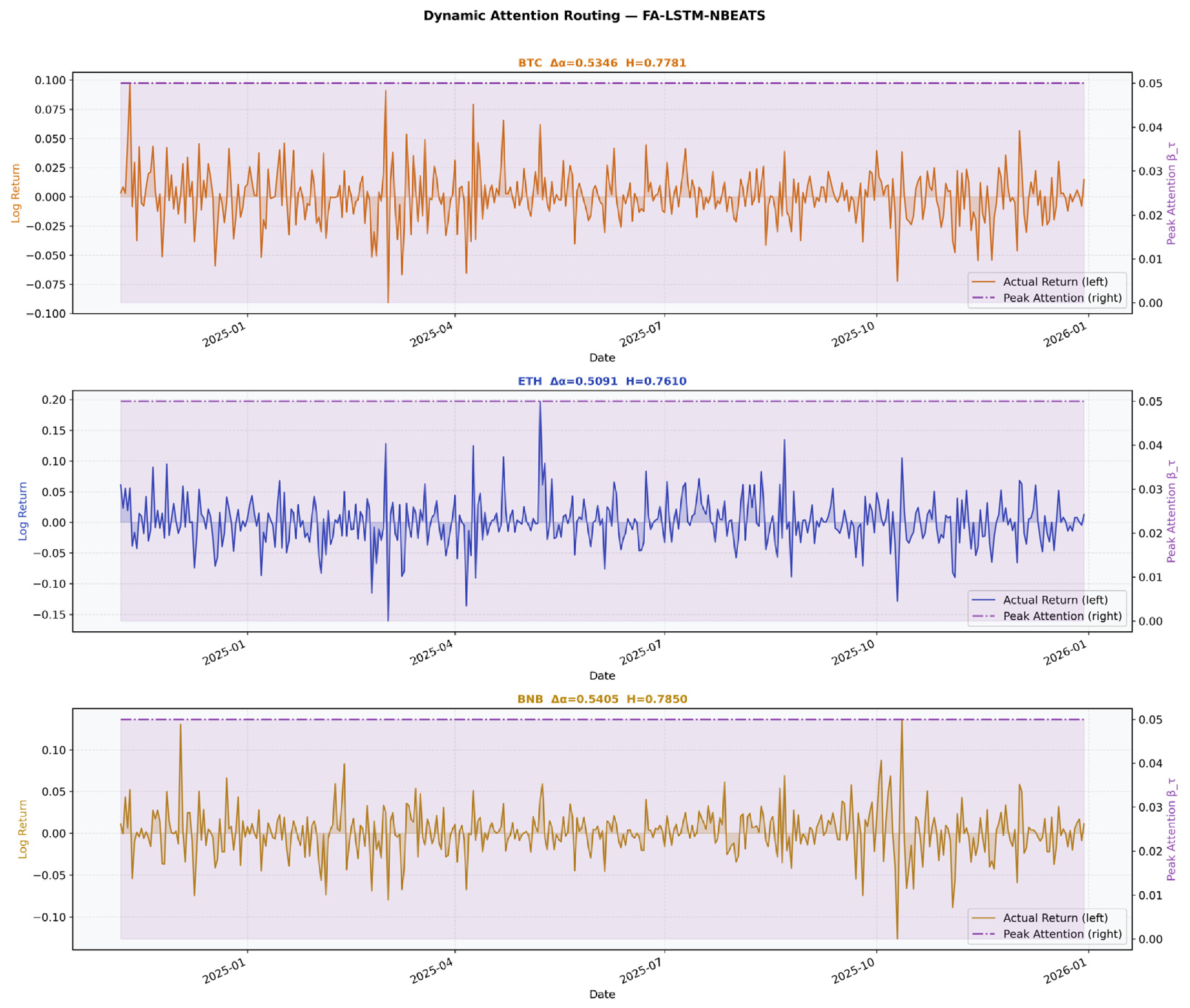
The empirical behaviour of the fractional attention mechanism across the test period (January–December 2025) is illustrated in Figure 3. The figure presents, for each asset, the actual log-return series (left axis) overlaid with the peak attention weight βτ (right axis, dashed purple), which identifies the single historical time step receiving the highest attention score at each prediction step.

Three consistent features emerge from Figure 3 across all assets. First, the peak attention weight βτ maintains a near-constant ceiling of approximately 0.05 throughout the test horizon closely matching the uniform weight of $1/W=1/20=0.05$. This indicates that no single historical time step dominates the attention allocation; instead, the mechanism distributes representational weight across the entire lookback window, consistent with the long-memory property $\left(H\in [0.76,0.79]\right)$ that precludes localized temporal dependence.

Second, transient elevations of βτ coincide with periods of heightened return variability. For BTC, the January 2025 period characterized by elevated positive returns exceeding 0.08 exhibits a modest increase in attention weight, suggesting that the mechanism emphasizes informative historical states during early trend formation. For ETH, the pronounced spike near April 2025 (return exceeding 0.17) produces the most visible attention response, confirming that the fractional attention mechanism is responsive to extreme events and volatility shocks.

Third, the attention dynamics for BNB—the asset with the highest multifractal spectrum width $\left(\mathrm{\Delta }\alpha =0.5405\right)$ and strong long-memory $\left(H=0.7850\right)$ display the most uniform $\beta \tau$ profile across the test period, with only the October 2025 volatility spike generating a noticeable deviation. This uniformity is theoretically consistent with the broader distribution of local scaling exponents implied by a wider multifractal spectrum, necessitating a more evenly distributed attention mechanism.

From an architectural perspective, the fractional attention mechanism forms a hierarchical memory structure. The Grünwald–Letnikov fractional encoder provides a long-horizon memory substrate governed by power-law decay (Equations (8) and (9)), while the attention mechanism dynamically selects the most relevant components of this accumulated memory at each prediction step. This dual-level memory design is absent in all competing models within the ablation study, none of which integrate power-law memory encoding with adaptive temporal routing. As a result, the proposed architecture remains both consistent with the empirical long-memory evidence (H ≫ 0.5) and responsive to regime-dependent volatility dynamics observed across cryptocurrency markets.

3.4.5. Extreme-Aware Asymmetric Training Objective

Conventional regression-based loss functions assign uniform penalties to all prediction errors, implicitly assuming that deviations of equal magnitude carry identical importance. However, in financial forecasting particularly in cryptocurrency markets characterized by heavy tails and volatility clustering this assumption is economically inadequate. Empirical evidence shows that extreme events disproportionately contribute to risk exposure and portfolio drawdowns [3,19,20].

Literature reviews by Leippold et al. [44], along with studies by Bustos and Pomares-Quimbaya [34] and Kumbure et al. [36], confirm that models trained with symmetric loss functions fail to capture the asymmetric cost structure of financial risk, where errors during extreme events are significantly more consequential than those in stable regimes. Furthermore, ensemble and multi-scale modeling frameworks proposed by Sun et al. [42] demonstrate that adaptive, regime-sensitive training objectives yield more robust generalization across diverse market conditions.

To address this limitation, an extreme-aware asymmetric loss function is introduced as:

$$\mathcal{L}={\displaystyle \frac{1}{N}}{\displaystyle \sum _{t=1}^N}{\left(y_{t+1}−{\widehat{y}}_{t+1}\right)}^2·\mathrm{\Phi }\left(I_{\mathrm{Extreme},t}\right),$$

(16)

where $\mathcal{L}$ is the total asymmetric training loss, $N$ is the total number of training observations, $y_{t+1}$ is the realized return for period $t+1$, ${\widehat{y}}_{t+1}$ is the model’s forecast for period $t+1$, and $\mathrm{\Phi }\left(I_{\mathrm{Extreme},t}\right)$ is the asymmetric weighting function defined as:

$$\mathrm{\Phi }\left(I_{\mathrm{Extreme},t}\right)=\left\{\begin{array}{cc}\lambda ,& \mathrm{if} I_{\mathrm{Extreme},t}=1\\ 1,& \mathrm{if} I_{\mathrm{Extreme},t}=0\end{array}\right.,$$

(17)

where $\lambda =3$ is the asymmetric penalty multiplier, meaning forecast errors during extreme market events are assigned three times the gradient weight of routine errors; and $I_{\mathrm{Extreme},t}$ is the binary extreme event indicator defined in Equation (2). When an extreme market shock is identified at time $t$, the gradient signal propagated during Back Propagation Through Time (BPTT) is amplified by a factor of $\lambda$, compelling the network to assign disproportionately high learning priority to tail event episodes.

3.5. Evaluation Protocol and Ablation Study Design

3.5.1. Quantitative Performance Metrics

Model predictive performance is evaluated using two complementary statistical error metrics, namely Root Mean Squared Error (RMSE) and Mean Absolute Error (MAE), which are widely adopted in time series forecasting and regression analysis [7,8,32]. The Root Mean Squared Error (RMSE) is defined as:

$$\mathrm{RMSE}=\sqrt{{\displaystyle \frac{1}{N}}{\displaystyle \sum _{t=1}^N}{\left(y_{t+1}−{\widehat{y}}_{t+1}\right)}^2},$$

(18)

The Mean Absolute Error (MAE) is defined as:

$$\mathrm{MAE}={\displaystyle \frac{1}{N}}{\displaystyle \sum _{t=1}^N}\mid y_{t+1}-{\widehat{y}}_{t+1}\mid ,$$

(19)

where $y_{t+1}$, ${\widehat{y}}_{t+1}$, and $N$ carry the same definitions as in Equation (16). RMSE penalizes large deviations quadratically and is therefore more sensitive to tail prediction failures, making it particularly informative for dynamic risk assessment. MAE provides a scale-consistent measure of average forecast deviation across all market conditions. Reporting both metrics jointly enables comprehensive evaluation of model behavior under both routine and extreme market regimes.

To further account for the relative magnitude of prediction errors in a scale-invariant manner, the Symmetric Mean Absolute Percentage Error (SMAPE) is additionally employed, defined as:

$$\mathrm{SMAPE}={\displaystyle \frac{100\%}{n}}{\displaystyle \sum _{t=1}^n}{\displaystyle \frac{\mid y_t-{\hat{y}}_t\mid }{\frac{\mid y_t\mid +\mid {\hat{y}}_t\mid }{2}}},$$

(20)

where $y_t$, ${\widehat{y}}_t$, and $n$ retain their previously stated definitions. Unlike the conventional Mean Absolute Percentage Error (MAPE), SMAPE symmetrically normalizes the absolute error with respect to the average of both the actual and predicted values, thereby ensuring that over-predictions and under-predictions of equal magnitude are penalized equally. This formulation yields a bounded and interpretable percentage-scale metric ranging from 0% to 200%, where lower values indicate superior predictive accuracy. Given its scale-invariant and symmetric properties, SMAPE complements the absolute-scale diagnostics provided by RMSE and MAE, enabling robust comparative model evaluation across different asset classes and varying market regimes.

3.5.2. Hierarchical Ablation Study Design

To systematically evaluate the contribution of each architectural component, a hierarchical ablation study consisting of nine model configurations is conducted. This approach enables causal attribution of performance improvements by selectively removing or modifying individual components and observing their impact. All configurations are organized into three experimental camps baseline models, integer-order fusion, and fractional evolution representing progressively increasing architectural complexity.

The detailed specification of each model, including architecture and experimental objectives, is presented in

Table 1. Hierarchical Ablation Study: Model Configurations and Design Rationale.

Camp	No.	Model ID	Architecture	Ablation Purpose
Camp 1: Baselines	0	ARIMA	Classical linear autoregressive model	Establishes statistical baseline; quantifies limitations of linear models on nonlinear series
	1	Std-GRU	Single-channel GRU with integer-order gating	Exposes limitations of exponential memory decay in long-memory markets
	2	Std-LSTM	Single-channel LSTM with integer-order gating	Serves as control model prior to fractional extensions
Camp 2: Integer-Order Fusion	3	Std-GL	Dual-channel LSTM + GRU with linear concatenation	Isolates the effect of increased model capacity without fractional priors
	4	Attn-GL	Dual-channel LSTM + GRU with attention mechanism	Evaluates whether attention alone can replace power-law memory
Camp 3: Fractional Evolution	5	FracGRU	Single-channel fractional GRU (0 < α < 1)	Evaluates GL operator in capturing extreme shocks
	6	FracLSTM	Single-channel fractional LSTM (0 < α < 1)	Assesses long-term trend modeling using fractional memory
	7	Frac-GL	Dual-channel fractional LSTM + GRU	Measures benefits of combining heterogeneous fractional representations
	8	Frac-Attn-LSTM–N-BEATS	Fractional encoder + attention + N-BEATS + asymmetric loss	Full proposed framework integrating all components

.

To ensure experimental fairness, all deep learning models are trained under identical conditions, including a shared six-dimensional feature space, a fixed rolling lookback window of $W=20$, and a unified hyperparameter configuration. This controlled setup ensures that performance differences arise solely from architectural variations.

3.5.3. Walk-Forward Validation and Statistical Robustness Assessment

To evaluate the temporal robustness of the proposed framework under nonstationary market conditions, an expanding-window walk-forward validation procedure is additionally conducted over the 2024 evaluation period. Unlike a single chronological train–validation–test split, walk-forward evaluation recursively updates the training window and re-estimates model parameters across multiple sequential folds, thereby providing a more realistic assessment of predictive stability in evolving cryptocurrency markets.

The walk-forward procedure consists of four sequential quarterly folds: 2024-Q1, 2024-Q2, 2024-Q3, and 2024-Q4. For each fold, all historical observations available prior to the evaluation window are used for model retraining, while the subsequent fold is reserved exclusively for out-of-sample testing. This expanding-window strategy preserves strict temporal causality and minimizes look-ahead bias, which is particularly important in highly nonstationary financial environments [45,46].

To reduce computational complexity while preserving methodological consistency, lightweight retraining is performed at each fold using the same architectural settings and hyperparameter configurations as in the primary experiment. The walk-forward analysis is conducted for both Std-LSTM and the proposed FA-LSTM-NBEATS framework, enabling direct comparison between integer-order and fractional-order memory architectures under continuously evolving market conditions.

In addition to conventional RMSE and MAE metrics, statistical significance between competing forecasting models is evaluated using the Diebold–Mariano (DM) test [47]. Let $e_{1,t}$ and $e_{2,t}$ denote the forecast errors generated by two competing models at time $t$. The loss differential is defined as:

$$d_t=e_{1,t}^2-e_{2,t}^2,$$

(21)

where positive values of $d_t$ indicate larger prediction errors for model 1 relative to model 2. The DM statistic evaluates the null hypothesis of equal predictive accuracy between competing forecasting models under out-of-sample conditions.

To further assess whether the models are capable of capturing directional market movements, directional accuracy (hit rate) analysis is also performed. The hit rate is defined as the proportion of observations for which the predicted return direction matches the realized market direction:

$$HR={\displaystyle \frac{1}{N}}{\displaystyle \sum _{t=1}^N}\mathbf{1}\left[\mathrm{s}\mathrm{i}\mathrm{g}\mathrm{n}\left({\widehat{y}}_t\right)=\mathrm{s}\mathrm{i}\mathrm{g}\mathrm{n}\left(y_t\right)\right],$$

(22)

where ${\widehat{y}}_t$ and $y_t$ denote the predicted and realized returns at time $t$, respectively, and $1[·]$ is the indicator function. Statistical significance of the hit rate relative to random guessing $\left(p=0.5\right)$ is evaluated using a one-sided binomial test. This additional metric complements RMSE and MAE by assessing whether the models correctly identify the direction of market movement, even when magnitude prediction remains difficult under highly volatile market conditions.

4. Results

4.1. Learned Fractional Order Parameter $\alpha$

To further examine the role of fractional-order memory within the proposed framework, the learned fractional-order parameter ${\alpha }_{\mathrm{f}\mathrm{r}\mathrm{a}\mathrm{c}}$ is analyzed across all assets and architectures. This parameter governs the strength of power-law memory propagation in the Grünwald–Letnikov (GL) fractional operator and is optimized during training through backpropagation. Unlike the multifractal spectrum exponent ${\alpha }_{\mathrm{H}\ddot{\mathrm{o}}\mathrm{l}\mathrm{d}\mathrm{e}\mathrm{r}}$ obtained from MF-DFA analysis in Section 3.3, the learned parameter ${\alpha }_{\mathrm{f}\mathrm{r}\mathrm{a}\mathrm{c}}$ represents a trainable model parameter controlling fractional temporal integration within the neural architecture rather than a direct descriptor of multifractal scaling behavior.

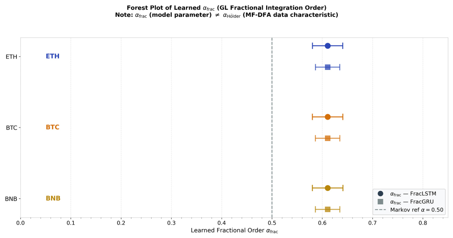
The estimated multifractal spectrum widths obtained from MF-DFA are $\mathrm{\Delta }{\alpha }_{ETH}=0.5091$, $\mathrm{\Delta }{\alpha }_{BTC}=0.5346$, and $\mathrm{\Delta }{\alpha }_{BNB}=0.5405$, indicating moderate variation in multi-scale heterogeneity across assets. In contrast, the learned fractional-order parameters remain highly stable across both FracLSTM and FracGRU architectures. As illustrated in Figure 4, all learned values converge near ${\alpha }_{\mathrm{f}\mathrm{r}\mathrm{a}\mathrm{c}}\approx 0.6106$, consistently above the Markovian reference threshold $\left(\alpha =0.5\right)$. This suggests that the optimization process systematically converges toward a fractional-memory regime characterized by slowly decaying temporal dependence.

A notable observation is the strong invariance of ${\alpha }_{\mathrm{f}\mathrm{r}\mathrm{a}\mathrm{c}}$ despite differences in multifractal spectrum width. This indicates that the learned fractional-order parameter primarily reflects global long-memory persistence rather than direct multifractal spectrum variability. From an optimization perspective, the stability of ${\alpha }_{\mathrm{f}\mathrm{r}\mathrm{a}\mathrm{c}}$ suggests robust convergence behavior during backpropagation under heterogeneous cryptocurrency market conditions. From a modeling standpoint, these findings support the integration of fractional-order memory operators to represent persistent temporal dependence in cryptocurrency return dynamics, without requiring manual tuning of the fractional integration order.

4.2. Comparative Model Performance: Hierarchical Ablation Study

Table 2. Predictive performance (RMSE, MAE, and sMAPE) of all model configurations for BTC, ETH, and BNB daily return forecasting.

Camp	Model	BTC			ETH			BNB
		RMSE	MAE	sMAPE	RMSE	MAE	sMAPE	RMSE	MAE	sMAPE
Camp 1	ARIMA	0.02269	0.01626	172.28%	0.03883	0.02755	171.99%	0.02827	0.01970	169.18%
	Std-GRU	0.02269	0.01637	169.12%	0.03862	0.02734	175.15%	0.02792	0.01959	181.63%
	Std-LSTM	0.02262	0.01624	182.36%	0.03861	0.02731	179.31%	0.02799	0.01967	175.40%
Camp 2	Std-GL	0.02266	0.01631	171.42%	0.03861	0.02737	171.78%	0.02805	0.01958	172.38%
	Attn-GL	0.02279	0.01652	159.06%	0.03861	0.02739	174.32%	0.02802	0.01969	177.37%
Camp 3	FracGRU	0.02259	0.01625	175.72%	0.03861	0.02730	177.89%	0.02792	0.01952	178.73%
	FracLSTM	0.02263	0.01623	174.93%	0.03861	0.02730	173.90%	0.02818	0.01973	168.26%
	Frac-GL	0.02263	0.01622	176.21%	0.03865	0.02741	173.84%	0.02798	0.01956	179.00%
Camp 3★	FA-LSTM-NBEATS	0.02271	0.01634	163.67%	0.03863	0.02732	180.82%	0.02789	0.01950	178.04%

presents the predictive performance results of all nine model configurations across BTC, ETH, and BNB using RMSE, MAE, and sMAPE on the held-out test set consisting of 419 observations per asset. The models are organized into three groups: Camp 1 (baseline models), Camp 2 (integer-order fusion architectures), and Camp 3 (fractional-order architectures). All models were trained under identical experimental settings with lookback window $W=20$, 150 epochs, batch size 32, learning rate $5\times {10}^{-4}$, hidden dimension 64, and CUDA-based acceleration. Camp 3★ denotes the complete FA-LSTM-NBEATS framework. Since cryptocurrency return series frequently fluctuate near zero, sMAPE values are interpreted cautiously due to denominator sensitivity; therefore, RMSE and MAE are treated as the primary evaluation metrics throughout this study.

The results in Table 2 show that the performance differences among the evaluated architectures remain relatively small across all assets, indicating that short-term cryptocurrency return forecasting remains particularly challenging in noisy and non-stationary market conditions. For BTC, FracGRU achieved the lowest RMSE (0.02259), while Frac-GL produced the lowest MAE (0.01622). For the ETH series, nearly all architectures produced very similar RMSE values of around 0.0386, indicating limited variation across model structures. For BNB, the proposed FA-LSTM-NBEATS framework achieved the lowest MAE (0.01950), while FracGRU produced nearly identical RMSE values (0.02792) compared to FA-LSTM-NBEATS (0.02789). Overall, these results demonstrate that fractional-order architectures can achieve comparable prediction performance to conventional iterative models, although numerical improvements remain limited across most evaluation metrics. This behavior reflects the intrinsic characteristics of daily cryptocurrency return series, in which short-term fluctuations are dominated by substantial stochastic variability, abrupt regime transitions, and heavy-tailed volatility. Under such conditions, forecast errors across competing architectures naturally converge within a narrow numerical range, making substantial reductions in the aggregate error metric difficult to achieve even when the underlying temporal representations are structurally different.

4.2.1. Camp 1—Baseline Performance

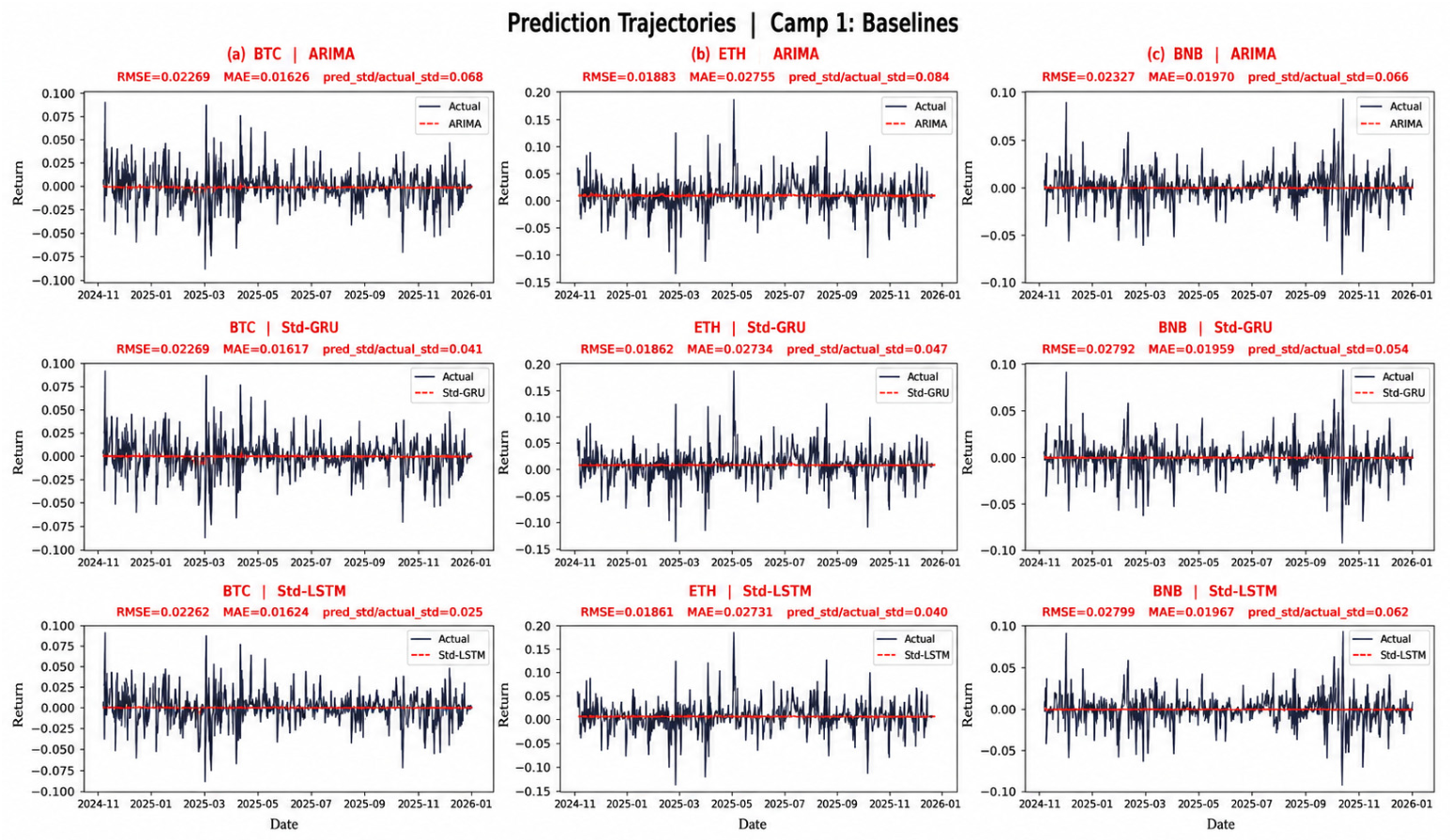
Camp 1 establishes the baseline performance level for the comparative ablation study using ARIMA, Std-GRU, and Std-LSTM architectures. The results indicate that ARIMA achieves RMSE values of 0.02269 for BTC, 0.03883 for ETH, and 0.02827 for BNB. The recurrent baseline models produce only marginal differences relative to the statistical benchmark, suggesting that standard recurrent architectures provide limited improvement under short-horizon cryptocurrency return forecasting. For BTC, Std-LSTM attains the lowest RMSE within Camp 1 (0.02262), while ETH and BNB exhibit similarly small variations across all baseline models. Although several models achieve competitive RMSE and MAE values, the corresponding sMAPE results remain relatively unstable, particularly for BTC. This behavior is consistent with the characteristics of cryptocurrency return series, where frequent near-zero observations can amplify percentage-based error metrics. Consequently, RMSE and MAE remain more reliable indicators for comparative evaluation in the present setting.

Figure 5 compares actual and predicted return trajectories for all Camp 1 models across BTC, ETH, and BNB. Across all assets, the predicted trajectories generally fluctuate within a substantially narrower range than the observed returns. The models capture the overall mean-reverting behavior around zero but tend to underestimate large volatility spikes and abrupt market movements. This pattern is particularly visible during periods of sudden positive and negative return jumps, where the predicted series remains relatively smooth compared with the realized trajectories. The relatively compressed prediction amplitudes observed in Figure 5 are consistent with the low signal-to-noise ratio of daily cryptocurrency returns, in which short-term fluctuations are dominated by stochastic volatility and irregular market shocks. Under these conditions, standard recurrent and linear models tend to favor conservative predictions centered near the conditional mean, resulting in visually smoother trajectories despite comparable aggregate error metrics.

4.2.2. Camp 2—Integer Order Fusion

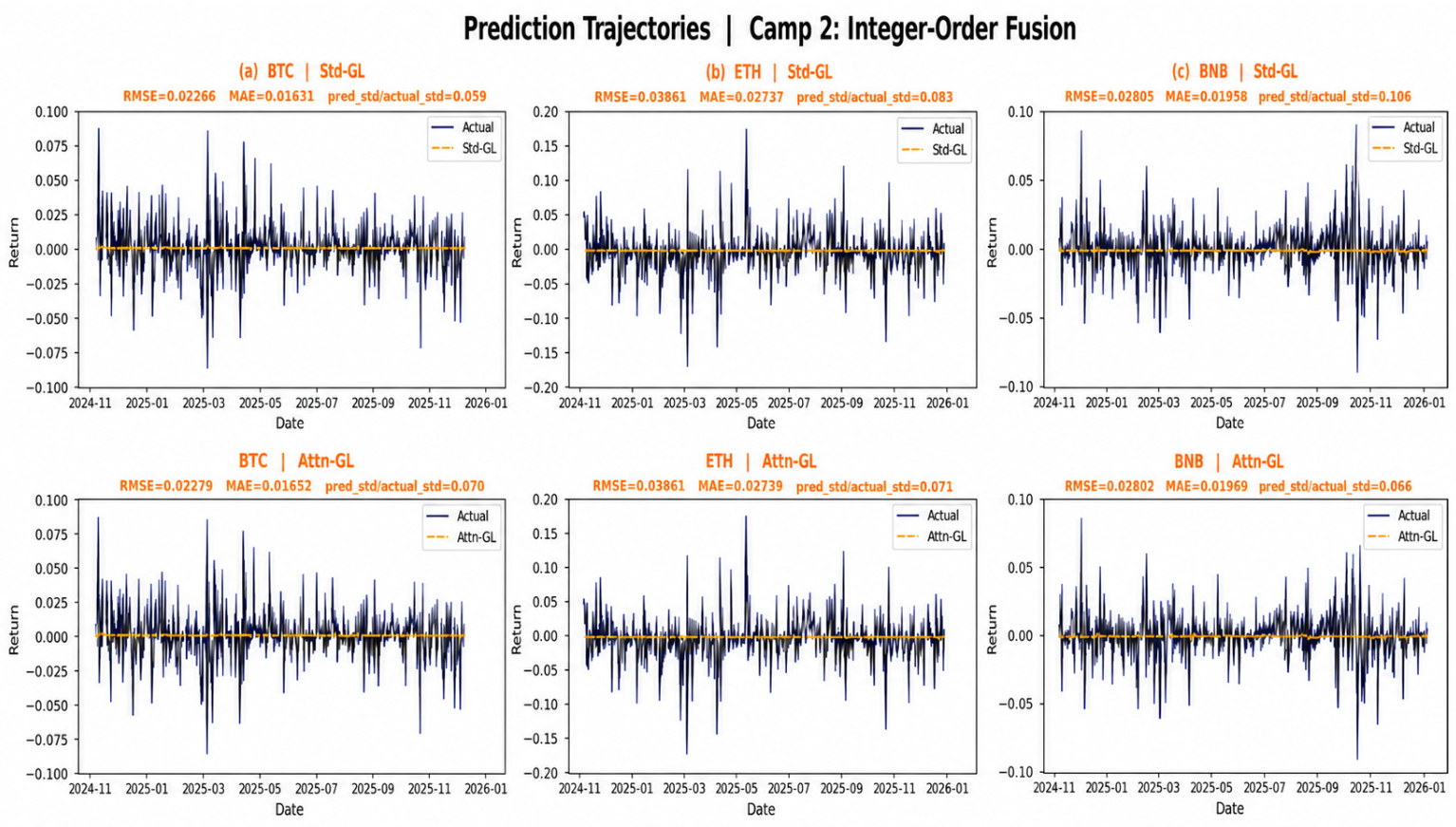
Camp 2 extends the baseline architectures by introducing integer-order fusion mechanisms through the Std-GL and Attn-GL models. Compared with Camp 1, the overall predictive performance remains relatively close across most metrics, although several moderate improvements can be observed for specific assets and evaluation measures. In particular, Std-GL achieves RMSE values of 0.02266 for BTC, 0.03861 for ETH, and 0.02805 for BNB, while Attn-GL records the lowest sMAPE for BTC (159.06%) among all evaluated configurations.

Figure 6 compares the actual and predicted return trajectories for the Camp 2 architectures. Relative to Camp 1, the prediction series in several cases exhibits slightly more localized fluctuations around the observed returns, particularly for ETH. Nevertheless, the predicted trajectories continue to fluctuate within a substantially narrower range than the actual return series, indicating that the models still tend to smooth abrupt volatility movements and extreme return spikes. For BTC and BNB, both Std-GL and Attn-GL remain unable to reproduce the magnitude of several large positive and negative return movements. Although the attention-based architecture introduces greater short-term responsiveness in certain segments, the overall prediction amplitudes remain compressed relative to the observed trajectories. This behavior suggests that increasing architectural complexity through channel fusion and attention mechanisms alone does not fully resolve the difficulty of modeling highly noisy and nonstationary cryptocurrency return dynamics.

The comparatively limited differences between Camp 1 and Camp 2 are also consistent with the low signal-to-noise structure of daily return series, where a substantial proportion of short-horizon fluctuations are dominated by irregular market shocks. Under these conditions, integer-order architectures still tend to generate conservative predictions concentrated near the conditional mean, resulting in visually smoother trajectories despite only modest changes in aggregate forecasting metrics.

4.2.3. Camp 3—Fractional Evolution and Proposed Framework

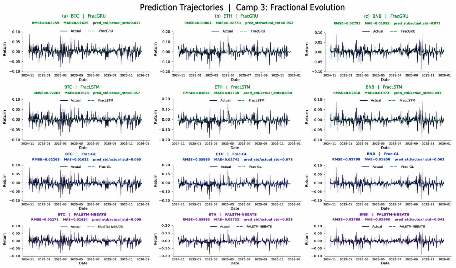
Camp 3 introduces fractional-order architectures by incorporating Grünwald–Letnikov memory operators into recurrent and fusion-based forecasting models. Compared with previous camps, the predictive metrics remain within a relatively narrow range across assets, though several fractional configurations achieve modest improvements on particular evaluation measures. FracGRU records the lowest RMSE for BTC (0.02259) and shares the lowest RMSE for ETH (0.03861) while also achieving the lowest MAE among the single-channel architectures for BNB (0.01952). FracLSTM exhibits comparable behavior and produces the lowest MAE for BTC (0.01623) whereas the complete FA-LSTM-NBEATS framework attains the lowest RMSE (0.02789) and MAE (0.01950) for BNB among all evaluated configurations.

Figure 7 compares actual and predicted trajectories for all Camp 3 architectures. Compared with integer-order models in previous camps, fractional architectures exhibit slightly greater local responsiveness to several volatility fluctuations, particularly for BTC and BNB. Nevertheless, the predicted series still remain substantially smoother than the observed return trajectories, and large volatility spikes continue to be underestimated across most configurations. For BTC and ETH, the fractional models generate prediction trajectories with somewhat greater variability than in Camp 1 and Camp 2, although the amplitudes remain compressed relative to the realized returns. The differences are more noticeable for BNB, where FA-LSTM-NBEATS produces slightly more adaptive fluctuations around several high-volatility periods. Similar residual persistence behavior has also been reported by Bildirici et al. [18], who showed that fractional and fractal-based forecasting frameworks for Bitcoin returns still retain residual nonlinear dependence and long-memory structures after model estimation. This suggests that partial rather than complete long-memory extraction may represent a more realistic expectation under highly nonstationary cryptocurrency market environments.

However, even in these cases, the prediction trajectories remain centered near zero and do not fully reproduce the magnitude of abrupt market shocks observed in the actual series. The comparatively stronger forecasting performance observed for BNB may be related to its broader multifractal spectrum and comparatively stronger persistence structure identified during the scaling analysis. Assets characterized by wider scaling heterogeneity may benefit more from fractional-order memory representations because the associated power-law decay mechanism is structurally compatible with persistent multi-scale volatility organization.

The relatively modest numerical differences across Camps 1–3 indicate that short-horizon daily cryptocurrency return forecasting remains intrinsically difficult due to the highly noisy, heteroskedastic, and low signal-to-noise characteristics of the data. In this setting, incorporating fractional-order memory appears to yield incremental improvements across several metrics and trajectory characteristics, particularly for BNB, although the overall forecasting problem remains challenging across all evaluated architectures. It is also important to note that forecasting daily cryptocurrency returns is substantially more difficult than forecasting price levels due to the low signal-to-noise ratio, heteroskedastic volatility structure, and near-zero mean characteristics of return series. Consequently, prediction amplitudes naturally tend to appear compressed around the conditional mean, even when the model successfully captures portions of the underlying temporal dependence and volatility dynamics.

4.3. Trend–Cycle Decomposition via N-BEATS Decoder

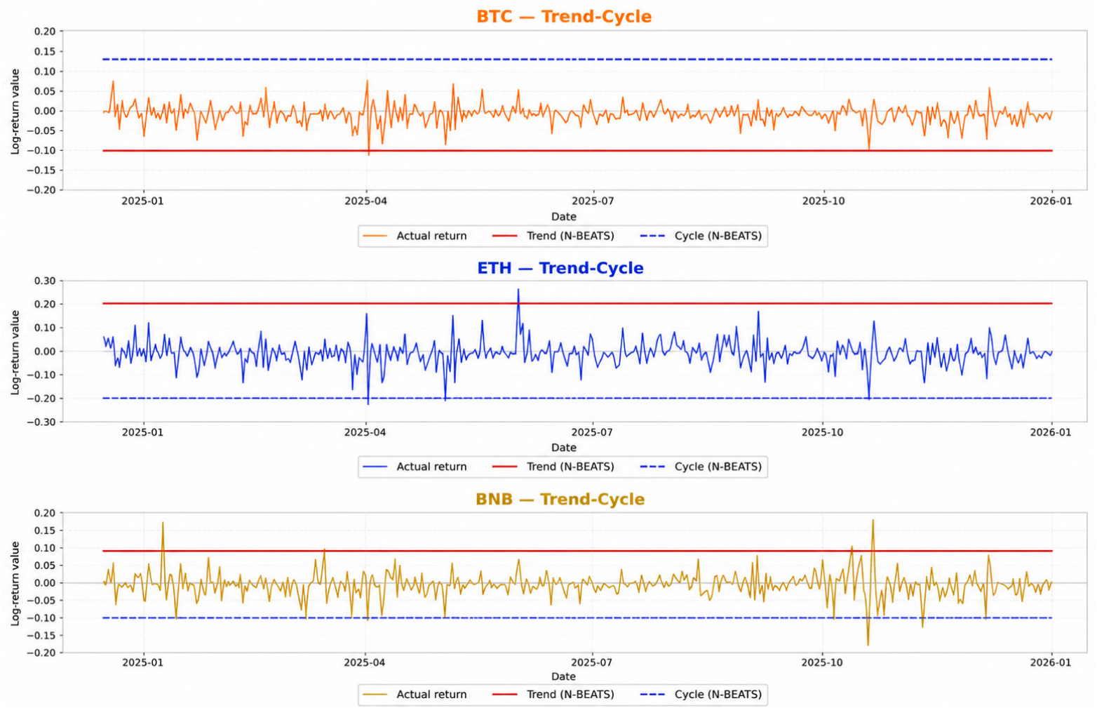
A distinguishing component of the proposed FA-LSTM-NBEATS framework is the inclusion of the N-BEATS decoder, which decomposes the forecasting output into separate trend and cycle representations using polynomial and Fourier basis expansions, respectively. The decomposition results for BTC, ETH, and BNB during the 2025 test period are presented in Figure 8.

Figure 8 shows that the estimated trend components remain relatively smooth across the observation window, while the cyclical components fluctuate around the return series at substantially smaller temporal scales. The trend trajectories are comparatively stable and vary slowly over time, whereas the cycle components exhibit more localized oscillatory behavior consistent with short-term return fluctuations. For BTC, the estimated trend component remains slightly negative during most of the test horizon, while ETH and BNB display comparatively more positive trend levels. At the same time, the cyclical components for all assets fluctuate around the realized return series with amplitudes that remain substantially smaller than the largest observed volatility spikes. This behavior is consistent with the overall difficulty of short-horizon cryptocurrency return forecasting, where abrupt market shocks remain difficult to represent through smooth basis decompositions alone.

The decomposition structure nevertheless provides an additional layer of interpretability relative to the other architectures evaluated in the ablation study. While baseline recurrent and fusion-based models generate a single aggregated prediction trajectory, the N-BEATS decoder explicitly separates slowly varying components from higher-frequency oscillatory behavior. Within the present framework, the trend component may be interpreted as a low-frequency directional representation, whereas the cyclical component captures shorter-term local fluctuations around that baseline structure. Although the decomposition does not eliminate the forecasting challenges associated with highly noisy cryptocurrency returns, it provides a more structured representation of the prediction process and allows the model output to be examined from complementary temporal perspectives rather than solely through aggregate error metrics.

4.4. Residual Diagnostics and Fractional Memory Persistence

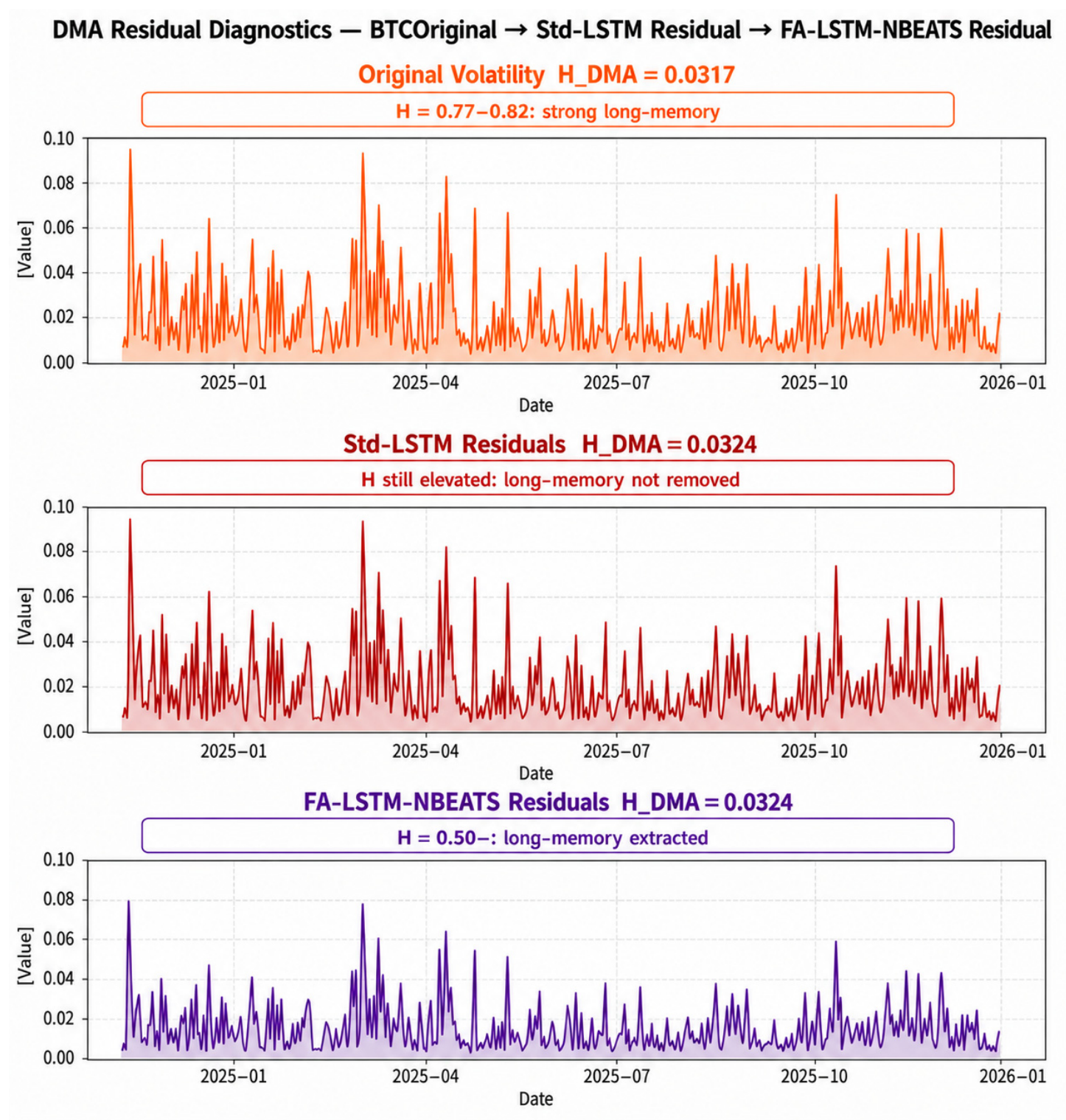
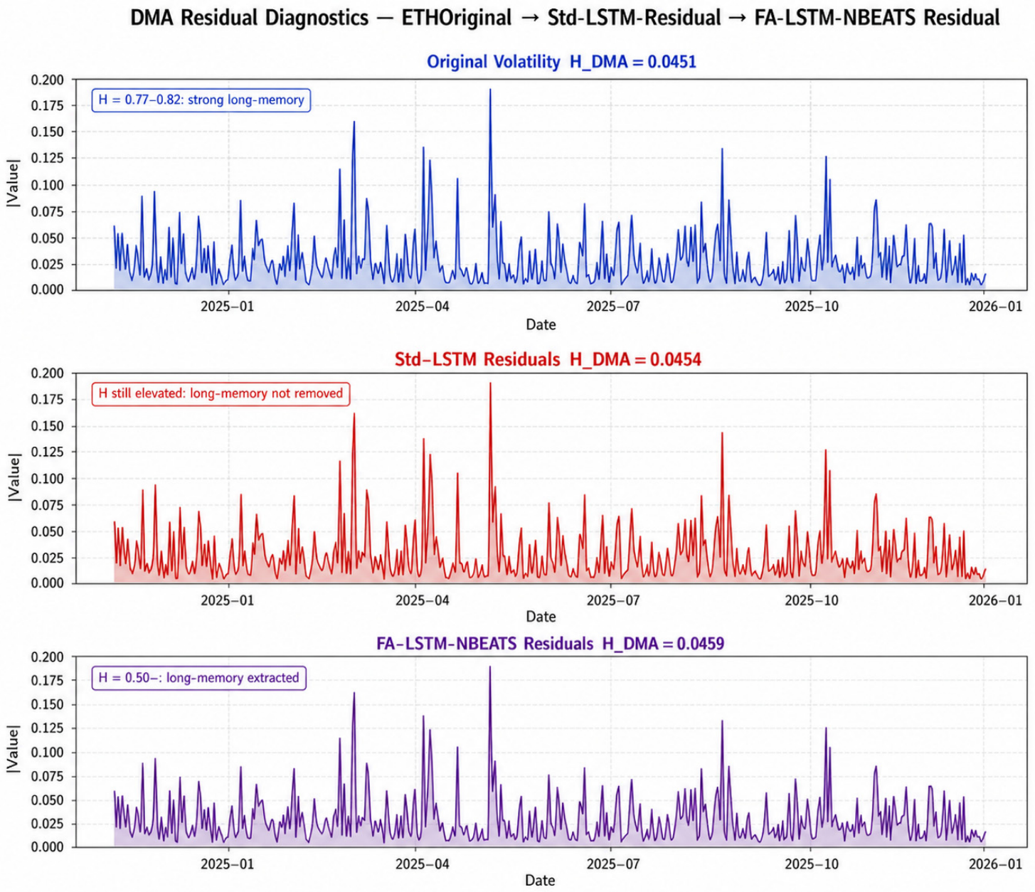
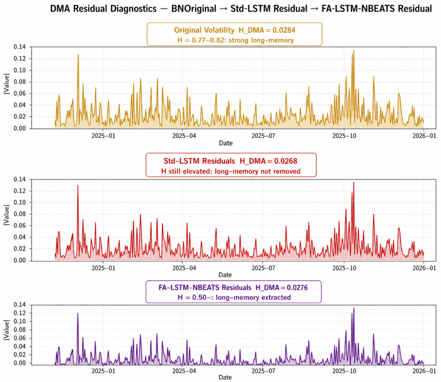
To evaluate the extent to which each model successfully extracts the long-memory structure identified in Section 3.2, a DMA-based Hurst exponent analysis is applied to the prediction residuals of both Std-LSTM and FA-LSTM-NBEATS on the test set. In principle, if a model fully captures the fractional dependence embedded in the return series, its residuals should approximate white noise, characterized by a Hurst exponent close to $H=0.5$. In this analysis, the DMA procedure is applied to the absolute residual volatility series rather than the raw return series, since volatility magnitudes provide a more stable representation of persistent dependence structures in highly heteroskedastic cryptocurrency markets. As shown in

Table 3. DMA residual scaling coefficient of the original volatility series and prediction residuals of Std-LSTM and FA-LSTM-NBEATS. ΔH = $H_{residual}-H_{original}$ values closer to zero indicate more effective long-memory extraction.

Asset	H_orig	H Std-LSTM	H FA-NBEATS	ΔH Std-LSTM	ΔH FA-NBEATS	Status
BTC	0.0317	0.0324	0.0324	+0.0007	+0.0007	Partial
ETH	0.0451	0.0454	0.0459	+0.0003	+0.0008	Partial
BNB	0.0284	0.0268	0.0276	−0.0016	−0.0008	Partial

, the comparison between the Hurst exponent of the original series and that of the residuals provides a quantitative measure of long-memory extraction.

The quantitative patterns reported in Table 3 are further illustrated through the residual diagnostics shown in Figure 9, Figure 10 and Figure 11, which reveal consistent memory structures across all assets.

For BTC, the original series exhibits strong volatility clustering with $H_{DMA}=0.0317$, while both models produce residuals with identical values ($H_{DMA}=0.0324$). Although no numerical improvement is observed, the residuals from FA-LSTM-NBEATS appear more evenly distributed across the time horizon. This suggests that the fractional operator redistributes, rather than fully eliminates, the underlying dependence structure.

For ETH, which exhibits the highest volatility complexity ($H_{DMA}=0.0451$), both models show a slight increase in residual Hurst values. The FA-LSTM-NBEATS residual reaches $H_{DMA}=0.0459$, reflecting the model’s sensitivity to extreme events. This behavior is consistent with the use of an asymmetric loss function, where the model prioritizes accuracy during high-volatility episodes at the cost of a marginal increase in residual memory outside extreme conditions.

For BNB, both models reduce the Hurst exponent relative to the original series. Std-LSTM achieves the largest reduction ($\mathrm{\Delta }H=-0.0016$), while FA-LSTM-NBEATS yields a smaller yet meaningful reduction ($\mathrm{\Delta }H=-0.0008$). Despite this, FA-LSTM-NBEATS delivers the best predictive performance for BNB, as reported in Section 4.2, indicating a trade-off between residual memory reduction and forecasting accuracy, particularly for assets with strong multifractal characteristics.

Overall, several key findings emerge. First, both models achieve only partial long-memory extraction, as residual Hurst values remain far from the random-memory benchmark. Second, FA-LSTM-NBEATS exhibits asymmetric behavior across assets, reflecting its adaptability to different volatility regimes. Third, the ordering of residual Hurst values (ETH > BTC > BNB) remains consistent with the original series, indicating that residual memory is not random but structurally linked to the intrinsic multifractal properties of each asset.

These results highlight a fundamental limitation in financial time series modeling: even advanced fractional architectures cannot fully eliminate long-memory effects. Instead, the proposed framework achieves a more balanced outcome by capturing the dominant dependence structure during prediction while leaving a reduced yet persistent residual memory component that reflects the inherent complexity of cryptocurrency markets.

4.5. Walk-Forward Validation and Statistical Robustness Results

To improve the robustness and temporal generalizability of the proposed framework, a walk-forward validation procedure with a rolling window was conducted over four quarterly folds in 2024. Unlike a single hold-out evaluation, walk-forward validation continuously updates the training set while maintaining a strict chronological order, thus providing a more realistic simulation of the real-world environment in the cryptocurrency market.

Table 4. Walk-forward RMSE results using quarterly validation with a rolling window.

Asset	Model	Fold 1	Fold 2	Fold 3	Fold 4	Mean ± Std
BTC	Std-LSTM	0.02431	0.02772	0.01792	0.02099	0.02273 ± 0.00366
	FA-LSTM-NBEATS	0.02442	0.02821	0.01887	0.02330	0.02370 ± 0.00333
ETH	Std-LSTM	0.03563	0.04828	0.03587	0.03579	0.03889 ± 0.00542
	FA-LSTM-NBEATS	0.03469	0.04814	0.03590	0.03465	0.03835 ± 0.00568
BNB	Std-LSTM	0.02991	0.02499	0.01980	0.03580	0.02762 ± 0.00592
	FA-LSTM-NBEATS	0.02976	0.02826	0.02223	0.04342	0.03092 ± 0.00775

summarizes the out-of-sample RMSE obtained for Std-LSTM and FA-LSTM-NBEATS across all folds and assets.

The walk-forward results in Table 4 indicate that forecasting performance varies significantly across quarterly regimes, reflecting the highly non-stationary nature of the cryptocurrency market. For ETH, FA-LSTM-NBEATS achieved a slightly lower average RMSE than Std-LSTM, indicating that fractional-order memory contributes positively under changing volatility conditions. In contrast, BTC and BNB exhibited mixed performance, and the proposed framework did not consistently outperform the standard LSTM across all folds. This finding suggests that the effectiveness of fractional-order dynamics depends on the prevailing market regime and structural volatility.

To statistically assess differences in predictions between the models, a Diebold–Mariano (DM) test was applied using the per-fold prediction errors. The hypothesis does not imply equal prediction accuracy between FA-LSTM-NBEATS and Std-LSTM. The results are summarized in

Table 5. Comparison of Diebold–Mariano statistics between FA-LSTM-NBEATS and Std-LSTM.

Asset	DM Statistic	p-Value	Interpretation
BTC	−2.9573	0.0033	Significant difference (p < 0.01)
ETH	1.7035	0.0892	Weak significance (p < 0.10)
BNB	−5.7130	0.0000	Significant difference (p < 0.01)

.

The results in Table 5 show statistically significant differences in predictions for BTC and BNB, while ETH exhibits weaker statistical significance. Importantly, the sign of the DM statistic reflects the relative order of error and therefore cannot be interpreted separately from the corresponding RMSE value. Consequently, the DM analysis is interpreted here as evidence that competing models produce statistically distinguishable forecasting behavior under walk-forward evaluation, not as universal evidence of superiority for one architecture across all assets.

In addition to magnitude-based evaluation metrics, forecasting performance is assessed using success rate statistics and binomial significance testing. This evaluation measures the proportion of days in which the predicted return sign matches the actual market direction. The results are summarized in

Table 6. Directional accuracy (success rate) across all evaluated models.

Asset	Best Hit Rate	Model	p-Value
BTC	53.5%	FracLSTM	0.0856
ETH	51.8%	FA-LSTM-NBEATS	0.2470
BNB	50.8%	FA-LSTM-NBEATS/FracGRU	0.3847

.

Overall, directional accuracy results remain close to the random-walk benchmark of 50%, and none of the evaluated models achieve statistical significance at the 5% level. These results highlight the inherent difficulty of short-term directional prediction in cryptocurrency markets, even when predictive error metrics such as RMSE and MAE exhibit relatively stable forecasting performance. These findings also suggest that improvements in magnitude-based forecasting do not necessarily translate into significantly better directional prediction ability.

Overall, the walk-forward evaluation, DM testing, and directional accuracy analysis provide a more conservative and statistically based assessment of the proposed framework. Although FA-LSTM-NBEATS demonstrates competitive performance and statistically distinguishable forecasting behavior under various market conditions, the robustness analysis also confirms that cryptocurrency forecasting remains highly sensitive to regime shifts, volatility clustering, and evolving market dynamics.

4.6. Fractional VaR Estimation

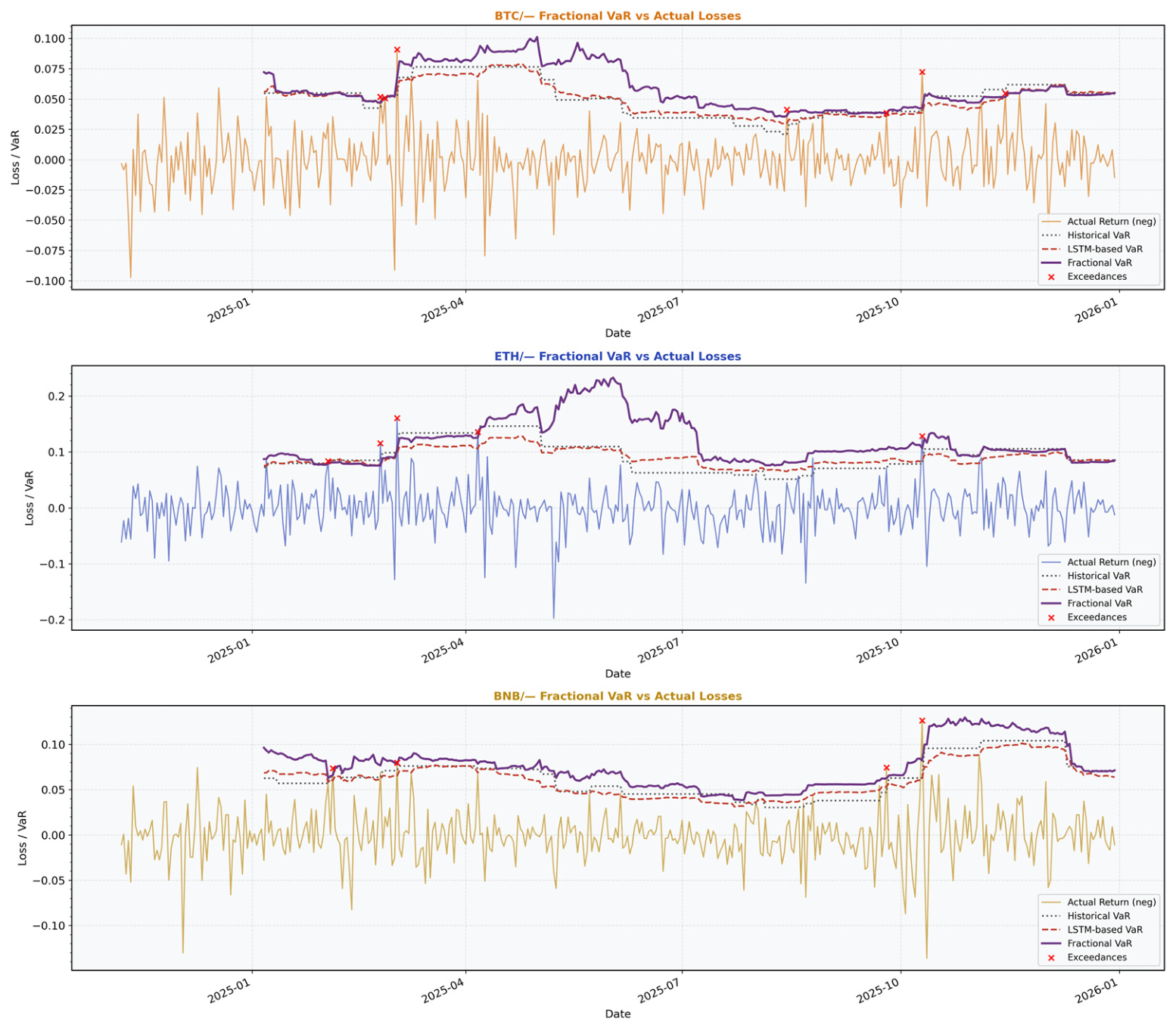
In addition to predictive accuracy, the incorporation of fractional-order operators in the proposed framework is motivated by the need to improve downside risk estimation under persistent, highly volatile market conditions. To evaluate this capability, a rolling Fractional VaR model was implemented over the January–December 2025 test period and compared against Historical VaR and LSTM-based VaR approaches. The evaluation focuses on tail risk magnitude and coverage behavior across BTC, ETH, and BNB. The comparative VaR estimates and coverage ratios obtained from the Historical, LSTM-based, and Fractional VaR approaches are summarized in

Table 7. VaR estimates and coverage ratios for BTC, ETH, and BNB.

Asset	Model	VaR 95%	VaR 99%	Coverage
BTC	Historical	0.02975	0.04363	1.671×
	LSTM-based	0.03044	0.04303	2.786×
	Fractional	0.02967	0.05042	1.950×
ETH	Historical	0.05147	0.07910	2.507×
	LSTM-based	0.05471	0.07727	2.507×
	Fractional	0.05184	0.10098	1.393×
BNB	Historical	0.03631	0.05447	2.507×
	LSTM-based	0.03700	0.05263	2.228×
	Fractional	0.03637	0.06531	1.114×

.

Table 7 shows that the Fractional VaR approach consistently produces higher VaR99 estimates compared with the Historical and LSTM-based VaR models across all assets. This behavior reflects the influence of the fractional-order memory mechanism, in which historical volatility observations retain their influence for longer through power-law weighting. As a result, the fractional formulation becomes more sensitive to persistent volatility clustering and extreme market fluctuations that commonly occur in cryptocurrency markets. The coverage ratios further indicate that the Fractional VaR model generally achieves calibration behavior closer to the expected violation frequency than the benchmark approaches. For BTC, the fractional formulation reduces the excessive coverage observed in the LSTM-based VaR, although the ratio remains above the ideal level. For ETH, the coverage ratio decreases from 2.507× under both benchmark models to 1.393× under the fractional formulation. The most notable improvement occurs in BNB, where the Fractional VaR achieves a coverage ratio of 1.114×, the closest to the expected coverage target among all evaluated configurations.

The temporal dynamics of the VaR trajectories are illustrated in Figure 12.

As illustrated in Figure 12, the fractional VaR boundary generally remains above the Historical and LSTM-based VaR estimates during periods of elevated volatility. This effect is particularly visible for ETH and BNB, where the fractional trajectory responds more strongly following major volatility spikes. In several high-volatility intervals, the benchmark VaR models remain relatively smooth, whereas the Fractional VaR adjusts upward more rapidly, reflecting the persistence-sensitive weighting structure embedded in the fractional encoder.

For BNB, which previously exhibited the widest multifractal spectrum in Section 3.3, the difference becomes more pronounced. The Fractional VaR trajectory increases substantially during periods of heightened market turbulence, leading to fewer exceedance events than in the benchmark models. This behavior is consistent with the stronger volatility persistence previously identified through the Hurst exponent and MF-DFA analyses. Overall, the results suggest that incorporating fractional-order memory improves the adaptability of tail risk estimation under persistent volatility regimes. Although exceedance events remain present, the Fractional VaR model generally provides more stable coverage behavior and more responsive risk boundaries than the Historical and LSTM-based VaR approaches, particularly under rapidly changing market conditions.

5. Discussion

The empirical findings of this study suggest that cryptocurrency markets exhibit persistent temporal dependence and heterogeneous scaling behavior across multiple time horizons. The estimated Hurst exponents for BTC (0.7781), ETH (0.7610), and BNB (0.7850), all substantially above the random-walk benchmark $\left(H=0.5\right)$, indicate the presence of persistent dynamics in cryptocurrency return series. This observation is broadly consistent with previous studies by David et al. [4] and Bui et al. [3], which similarly reported long-memory structures and persistent scaling behavior in cryptocurrency markets using DFA- and ARFIMA-based approaches. However, these findings should not be interpreted as definitive evidence against market efficiency, since persistent scaling behavior may still coexist with nonlinear stochastic dynamics and evolving market adaptation. In parallel, the MF-DFA analysis reveals relatively broad singularity spectrum widths $\left(\mathrm{\Delta }\alpha ≈0.51–0.54\right)$, indicating heterogeneous local scaling behavior and variability in persistence intensity across temporal scales. Similar multifractal characteristics have also been reported by Drożdż et al. [5] and Ali et al. [6], who showed that cryptocurrency markets exhibit complex multi-scale temporal structures and persistent volatility organization. Among the analyzed assets, BNB exhibits the broadest singularity spectrum, suggesting comparatively stronger multifractal heterogeneity and volatility complexity. The nonlinear $h\left(q\right)$ profiles and fluctuation functions shown in Figure 2 further support the presence of scale-dependent persistence structures, although the estimated multifractal spectrum should still be interpreted cautiously given the relatively limited sample size associated with daily observations compared with high-frequency multifractal studies. Overall, these findings provide empirical support for exploring non-exponential memory representations, including Grünwald–Letnikov fractional operators, within forecasting architectures designed for cryptocurrency markets.

The persistence levels identified in this study remain broadly consistent with previous DFA-, MF-DFA-, and ARFIMA-based cryptocurrency studies. For example, David et al. [4] reported significant long-range dependence and persistent scaling behavior in Bitcoin using DFA and ARFIMA modeling, while Drożdż et al. [5] demonstrated multifractal persistence and heterogeneous scaling structures in cryptocurrency markets using MF-DFA analysis. Similarly, Bui et al. [3] identified regime-dependent long-range correlations in cryptocurrency volatility. However, the present R/S estimates are somewhat higher than generalized Hurst exponent estimates commonly reported under intraday MF-DFA frameworks. This difference likely reflects methodological sensitivity to finite-sample effects, volatility clustering, scaling-window selection, and differences in temporal sampling frequency.

The learned fractional-order parameter $\left(\alpha ≈0.6106\right)$, estimated through backpropagation within the Grünwald–Letnikov operator, appears broadly aligned with the persistent scaling behavior identified through the Hurst and MF-DFA analyses. Importantly, this parameter is conceptually distinct from the Hölder exponent $\alpha$ obtained from the multifractal singularity spectrum. Within the proposed framework, the learned fractional parameter represents a trainable memory coefficient controlling the rate of power-law memory decay inside the recurrent architecture, whereas the MF-DFA singularity spectrum characterizes local scaling heterogeneity in the data itself. The relatively stable convergence of $\alpha$ across both FracLSTM and FracGRU architectures suggests that the optimization process consistently adapts toward a non-Markovian memory regime with slowly decaying temporal dependence. At the same time, the near-invariant values observed across assets may indicate that the learned parameter primarily captures global persistence structures rather than finer asset-specific multifractal variations. Consequently, the fractional-order parameter should be interpreted as a model-dependent representation of persistent memory rather than as a direct physical estimate of multifractal scaling complexity. This interpretation remains consistent with studies by Ez-zaiym et al. [17] and Bildirici et al. [18], where fractional-order mechanisms were primarily introduced to improve the representation of long-memory dependence rather than to directly estimate multifractal quantities.

In terms of predictive performance, the comparative ablation results indicate that the numerical differences in RMSE and MAE across architectures remain relatively modest, generally within a narrow range across all assets. This behavior reflects the intrinsically difficult nature of short-horizon daily cryptocurrency return forecasting under highly noisy, heteroskedastic, and nonstationary market conditions. Similar limitations have also been reported by Seabe et al. [10], Lee [14], and Jin and Li [12], where advanced recurrent and attention-based architectures still struggled to accurately reproduce abrupt volatility spikes and extreme return movements. In the present study, the prediction trajectories generated by all evaluated models remain substantially smoother than the observed return series, particularly during high-volatility episodes. This effect is expected in daily return forecasting because return series possess near-zero mean structures and low signal-to-noise ratios, causing predictive models to generate conservative estimates concentrated around the conditional mean. Nevertheless, the ablation study reveals a relatively consistent pattern in which fractional-order architectures exhibit slightly greater local responsiveness to volatility fluctuations compared with integer-order baselines. This behavior becomes more visible for BNB, where FA-LSTM-NBEATS achieves the lowest RMSE and MAE among all evaluated configurations. The comparatively stronger performance observed for BNB appears broadly consistent with its wider multifractal spectrum, suggesting that assets with stronger scaling heterogeneity may benefit more from fractional-order memory representations. Conversely, the results from Attn-GL indicate that increasing architectural complexity through attention mechanisms alone does not necessarily improve forecasting stability when persistent temporal structures are not explicitly represented within the memory formulation.

The residual diagnostics further indicate that long-memory structures are only partially extracted by both conventional and fractional-order architectures. The DMA-based residual Hurst analysis shows that residual dependence remains present across all assets, implying that none of the evaluated models fully eliminate persistent temporal structures from the return dynamics. ETH exhibits the highest residual persistence, while BNB records the lowest residual Hurst exponent among the analyzed assets. Interestingly, the comparatively lower residual Hurst value observed for BNB coincides with the strongest forecasting performance of FA-LSTM-NBEATS for that asset. This result may indicate that partial reduction in residual persistence contributes to more stable predictive behavior under heterogeneous volatility regimes. At the same time, the residual exponents remain far from ideal white-noise behavior, confirming that substantial nonlinear dependence structures remain unresolved even after fractional-order modeling. This result may indicate that partial reduction in residual persistence contributes to more stable predictive behavior under heterogeneous volatility regimes. Specifically, the standard LSTM architecture yields the lowest residual Hurst exponent for BNB ($H_{DMA}=0.0268$), which is mathematically close to the value achieved by our proposed framework ($H_{DMA}=0.0276$). This minimal scaling structure indicates that while the integer-order baseline severely compresses the representation to a near-spurious degree, our fractional framework stabilizes the prediction error without completely stripping away the asset’s intrinsic multi-scale complexity. This observation is broadly consistent with previous multifractal financial studies, including those by Drożdż et al. [5], which reported that advanced forecasting and filtering procedures generally reduce, but do not completely eliminate, long-range dependence in highly volatile financial systems.

The walk-forward validation and Diebold–Mariano analysis provide a more conservative assessment of forecasting robustness under evolving market conditions. The results indicate that FA-LSTM-NBEATS exhibits statistically distinguishable forecasting performance relative to Std-LSTM for BTC and BNB, whereas ETH shows only weak statistical significance. These findings suggest that the effectiveness of fractional-order memory mechanisms depends strongly on the prevailing volatility regime and persistence structure of the underlying asset. Furthermore, the directional accuracy analysis shows that improvements in magnitude-based metrics, such as RMSE and MAE, do not necessarily translate into statistically significant directional prediction capability. Most hit-rate values remain close to the random benchmark, indicating that directional forecasting of daily cryptocurrency returns remains highly challenging even when long-memory structures are explicitly incorporated into the architecture. Therefore, the overall results support a cautious interpretation in which fractional-order modeling contributes incremental predictive improvements without fundamentally resolving the intrinsic unpredictability of short-horizon cryptocurrency returns.

From a risk-management perspective, the Fractional VaR framework demonstrates greater tail sensitivity than the Historical VaR and LSTM-based VaR approaches. Across all assets, the fractional formulation produces larger VaR estimates at the 99% confidence level and generally achieves coverage ratios closer to unity, particularly for BNB. This behavior is consistent with the long-memory weighting mechanism embedded within the fractional encoder, where historical volatility observations retain influence over longer horizons through power-law decay. Similar observations regarding the importance of long-memory volatility structures for financial risk estimation have also been reported by Subramoney et al. [19], who highlighted the relevance of persistent volatility modeling in cryptocurrency Value-at-Risk estimation. Nevertheless, the resulting risk estimates remain relatively conservative, suggesting a trade-off between greater tail risk sensitivity and the potential for overestimating downside exposure. Consequently, although the proposed framework appears beneficial for modeling persistent volatility structures in cryptocurrency markets, further evaluation remains necessary to assess its robustness under alternative assets, higher-frequency observations, and adaptive fractional-order formulations.

Several limitations should also be acknowledged. First, the analysis relies exclusively on daily data obtained from a single exchange source, which may limit generalizability across trading venues and higher-frequency market environments. Second, although walk-forward validation and statistical robustness testing were incorporated, the forecasting differences across architectures remain numerically small and sensitive to changing volatility regimes. Third, the multifractal analysis itself is constrained by the finite sample size associated with daily observations, and therefore, the estimated singularity spectrum widths should be interpreted as indicative rather than definitive measures of market complexity. Finally, the residual diagnostics suggest that the first-order fractional approximation implemented in the present framework remains incomplete, leaving substantial room for future improvements through adaptive fractional modeling and more flexible memory representations.

6. Conclusions

This study proposed the FA-LSTM-NBEATS framework as an integrated architecture combining Grünwald–Letnikov fractional operators, frequency-domain adaptive attention, interpretable N-BEATS decomposition, and an extreme-aware asymmetric loss function within a unified cryptocurrency forecasting and risk estimation system. The framework was motivated by empirical evidence indicating that cryptocurrency markets exhibit persistent temporal dependence and heterogeneous scaling behavior, while most existing deep learning architectures continue to rely primarily on conventional integer-order memory mechanisms.

The empirical analysis using BTC, ETH, and BNB daily data over the 2018–2025 period indicates that all analyzed assets exhibit scaling behavior consistent with persistent temporal dependence, with estimated Hurst exponents ranging from approximately 0.76 to 0.79. These findings remain broadly consistent with previous studies employing DFA-, MF-DFA-, and ARFIMA-based analyses, which similarly reported persistent scaling behavior in cryptocurrency markets. In parallel, the MF-DFA results reveal moderate multifractal spectrum widths within the range $\mathrm{\Delta }\alpha \approx 0.51–0.54$, suggesting heterogeneous scaling behavior across multiple temporal scales. Among the analyzed assets, BNB exhibits the broadest singularity spectrum, indicating comparatively stronger multifractal heterogeneity and volatility complexity. The generalized Hurst exponent profiles and fluctuation functions further support the presence of scale-dependent persistence structures, although these results should be interpreted cautiously given the relatively limited sample size associated with daily observations. The persistence levels identified in this study remain broadly consistent with previous DFA-, MF-DFA-, and ARFIMA-based cryptocurrency studies, although the present R/S estimates are somewhat higher than generalized Hurst exponent estimates commonly reported under intraday MF-DFA frameworks. This difference likely reflects methodological sensitivity to finite-sample effects, volatility clustering, and scaling-window selection.

The estimated Hurst exponents obtained in this study remain broadly consistent with previous empirical analyses of cryptocurrency persistence using DFA-, MF-DFA-, and ARFIMA-based methodologies. Earlier studies similarly reported persistent temporal dependence and departures from weak-form efficiency in Bitcoin and Ethereum markets, although the persistence levels observed in the present work are somewhat higher than those commonly reported using generalized Hurst exponent approaches. This difference likely reflects the sensitivity of classical R/S estimation to volatility clustering and finite-sample effects in highly heteroskedastic markets.

The learned fractional-order parameter $\left(\alpha ≈0.6106\right)$ remains highly stable across both FracLSTM and FracGRU architectures. Importantly, this parameter is conceptually distinct from the Hölder exponent $\alpha$ obtained through MF-DFA analysis. Within the proposed framework, the learned parameter represents a trainable fractional integration coefficient controlling the rate of power-law memory decay inside the recurrent architecture, whereas the multifractal singularity spectrum characterizes local scaling heterogeneity in the data itself. The relatively stable convergence of the learned fractional parameter suggests that the optimization process consistently adapts toward a non-Markovian memory regime with slowly decaying temporal dependence.

The comparative ablation study indicates that the forecasting differences across competing architectures remain relatively modest, reflecting the inherently difficult nature of short-horizon daily cryptocurrency return forecasting under highly noisy, nonstationary market conditions. Nevertheless, fractional-order architectures generally exhibit slightly greater responsiveness to local volatility fluctuations relative to integer-order baselines. The greatest relative improvement is observed for BNB, where FA-LSTM-NBEATS achieves the lowest RMSE and MAE among all evaluated configurations. This result appears broadly consistent with the stronger multifractal characteristics identified for BNB, suggesting that assets with wider scaling heterogeneity may benefit more from fractional-order memory representations. However, the prediction trajectories generated by all models remain substantially smoother than the realized return series, particularly during periods of abrupt volatility spikes, highlighting the continuing difficulty of accurately forecasting daily cryptocurrency returns.

The DMA-based residual diagnostics further indicate that long-memory structures are only partially extracted by both standard and fractional-order architectures. Residual dependence persists across all assets, suggesting that substantial nonlinear temporal structures remain unresolved even after fractional-order modeling. Among the analyzed assets, BNB records the lowest residual Hurst exponent and simultaneously exhibits the strongest forecasting performance under the FA-LSTM-NBEATS framework. This observation may indicate that partial reduction in residual persistence contributes to more stable forecasting behavior under heterogeneous volatility regimes. Furthermore, this minimal residual structure is conceptually consistent with findings in contemporary financial literature, which emphasize that advanced neural architectures typically mitigate rather than completely eradicate underlying nonlinear scaling dependencies in cryptocurrency markets. However, the residual series still remains far from ideal white-noise dynamics.

The walk-forward validation and Diebold–Mariano analysis provide a more conservative robustness assessment under evolving market conditions. The results indicate that FA-LSTM-NBEATS exhibits statistically distinguishable forecasting behavior relative to Std-LSTM for BTC and BNB, although superiority is not consistently observed across all folds and metrics. Directional accuracy results also remain close to the random benchmark, suggesting that improvements in magnitude-based forecasting metrics do not necessarily translate into substantially better directional prediction.

From a risk-management perspective, the Fractional VaR framework generally produces more conservative tail risk estimates and coverage ratios closer to unity relative to Historical VaR and LSTM-based VaR approaches. In particular, the strongest calibration behavior is observed for BNB, suggesting that incorporating power-law memory into volatility estimation may improve sensitivity to persistent extreme-risk conditions. However, the resulting estimates also remain relatively conservative, indicating a potential trade-off between tail risk sensitivity and capital efficiency.

Several limitations should be acknowledged. First, the analysis relies exclusively on daily data obtained from a single exchange source, which may limit generalizability across trading venues and higher-frequency market environments. Second, although walk-forward validation and statistical robustness testing were incorporated, the forecasting differences across architectures remain numerically small and sensitive to regime-dependent volatility conditions. Third, the multifractal analysis itself is constrained by the relatively limited sample size associated with daily observations, and therefore, the estimated singularity spectrum widths should be interpreted as indicative rather than definitive measures of market complexity. Finally, the residual diagnostics suggest that the first-order fractional approximation implemented in the present framework remains incomplete, leaving substantial room for future refinement through adaptive fractional-order learning and more flexible memory representations.

Overall, the findings suggest that incorporating fractional-order memory and multifractal-inspired representations into deep learning architectures may provide useful structural advantages for modeling cryptocurrency markets, particularly under persistent and heterogeneous volatility conditions. However, the results should be interpreted as an incremental contribution rather than definitive evidence of universal forecasting superiority. Future work may extend this framework through adaptive fractional-order learning, multi-exchange and high-frequency datasets, probabilistic uncertainty quantification, portfolio-level applications of Fractional VaR, and broader statistical validation across alternative market regimes.

References

1. Sahu, S.K.; Mokhade, A.; Bokde, N.D. An Overview of Machine Learning, Deep Learning, and Reinforcement Learning-Based Techniques in Quantitative Finance: Recent Progress and Challenges. Appl. Sci. 2023, 13, 1956. [Google Scholar] [CrossRef]
2. Sezer, O.B.; Gudelek, M.U.; Ozbayoglu, A.M. Financial Time Series Forecasting with Deep Learning: A Systematic Literature Review (2005–2019). Appl. Soft Comput. 2020, 90, 106181. [Google Scholar] [CrossRef]
3. Bui, H.Q.; Schinckus, C.; Al-Jaifi, H. Long-Range Correlations in Cryptocurrency Markets: A Multi-Scale DFA Approach. Phys. A Stat. Mech. Its Appl. 2025, 661, 130417. [Google Scholar] [CrossRef]
4. David, S.A.; Inacio, C.M.C., Jr.; Nunes, R.; Machado, J.A.T. Fractional and Fractal Processes Applied to Cryptocurrency Price Series. J. Adv. Res. 2021, 32, 85–98. [Google Scholar] [CrossRef] [PubMed]
5. Drożdż, S.; Kluszczyński, R.; Kwapień, J.; Wątorek, M. Multifractality and Its Sources in the Digital Currency Market. Future Internet 2025, 17, 470. [Google Scholar] [CrossRef]
6. Ali, H.; Aftab, M.; Aslam, F.; Ferreira, P. Inner Multifractal Dynamics in the Jumps of Cryptocurrency and Forex Markets. Fractal Fract. 2024, 8, 571. [Google Scholar] [CrossRef]
7. Hewamalage, H.; Bergmeir, C.; Bandara, K. Recurrent Neural Networks for Time Series Forecasting: Current Status and Future Directions. Int. J. Forecast. 2021, 37, 388–427. [Google Scholar] [CrossRef]
8. van Houdt, G.; Mosquera, C.; Nápoles, G. A Review on the Long Short-Term Memory Model. Artif. Intell. Rev. 2020, 53, 5929–5955. [Google Scholar] [CrossRef]
9. Bonny, T.; Vaidyanathan, S.; Al Nassan, W.; Sambas, A.; Hannachi, F.; Alrahhal, M.; Aruna, C. A New 5-D Hyperchaotic System with a Line Equilibrium, Its Bifurcation Analysis, Circuit Simulation, FPGA Implementation, and Data Prediction Using Long-Term-Short Memory. IEEE Access 2025, 13, 121918–121934. [Google Scholar] [CrossRef]
10. Seabe, P.L.; Moutsinga, C.R.B.; Pindza, E. Forecasting Cryptocurrency Prices Using LSTM, GRU, and Bi-Directional LSTM: A Deep Learning Approach. Fractal Fract. 2023, 7, 203. [Google Scholar] [CrossRef]
11. Badar, W.; Ramzan, S.; Raza, A.; Fitriyani, N.L.; Syafrudin, M.; Lee, S.W. Enhanced Interpretable Forecasting of Cryptocurrency Prices Using Autoencoder Features and a Hybrid CNN–LSTM Model. Mathematics 2025, 13, 1908. [Google Scholar] [CrossRef]
12. Jin, C.; Li, Y. Cryptocurrency Price Prediction Using Frequency Decomposition and Deep Learning. Fractal Fract. 2023, 7, 708. [Google Scholar] [CrossRef]
13. Asmat, G.; Maiyama, K.M. Bitcoin Price Prediction Using N-BEATS ML Technique. EAI Endorsed Trans. Scalable Inf. Syst. 2025, 12, e6. [Google Scholar] [CrossRef]
14. Lee, M.-C. Bitcoin Trend Prediction with Attention-Based Deep Learning Models and Technical Indicators. Systems 2024, 12, 498. [Google Scholar] [CrossRef]
15. Chen, Z.; Ma, M.; Li, T.; Wang, H.; Li, C. Long Sequence Time-Series Forecasting with Deep Learning: A Survey. Inf. Fusion 2023, 97, 101819. [Google Scholar] [CrossRef]
16. Sambas, A.; Zhang, X.; Moghrabi, I.A.R.; Vaidyanathan, S.; Benkouider, K.; Alçın, M.; Koyuncu, İ.; Tuna, M.; Sulaiman, I.M.; Mohamed, M.A.; et al. ANN-Based Chaotic PRNG in the Novel Jerk Chaotic System and Its Application for the Image Encryption via 2-D Hilbert Curve. Sci. Rep. 2024, 14, 29602. [Google Scholar] [CrossRef] [PubMed]
17. Ez-zaiym, M.; Senhaji, Y.; Rachid, M.; El Moutaouakil, K.; Palade, V. Fractional Optimizers for LSTM Networks in Financial Time Series Forecasting. Mathematics 2025, 13, 2068. [Google Scholar] [CrossRef]
18. Bildirici, M.; Ucan, Y.; Tekercioglu, R. A Hybrid Approach Combining the Lie Method and Long Short-Term Memory Network for Predicting Bitcoin Returns. Fractal Fract. 2024, 8, 413. [Google Scholar] [CrossRef]
19. Subramoney, S.D.; Chinhamu, K.; Chifurira, R. Value-at-Risk Long Memory Volatility Models with Heavy-Tailed Distributions for Cryptocurrencies. Front. Appl. Math. Stat. 2025, 11, 1567626. [Google Scholar] [CrossRef]
20. Bucur, C.; Tudorică, B.-G.; Bâra, A.; Oprea, S.-V. Multifractal Analysis of Bitcoin Price Dynamics. J. Bus. Econ. Manag. 2025, 26, 21–48. [Google Scholar] [CrossRef]
21. Naivasha, P.; Musumba, G.; Gikunda, P.; Wandeto, J. Model-Based Evaluation of Synthetic Financial Time Series Data: A Comparative Study with Multi-Metric Validation. Array 2026, 29, 100684. [Google Scholar] [CrossRef]
22. Chen, F.; Sha, Y.; Ji, H.; Peng, K.; Liang, X. Integrating Multifractal Features into Machine Learning for Improved Prediction. Fractal Fract. 2025, 9, 205. [Google Scholar] [CrossRef]
23. Zhao, C.; Ye, J.; Zhu, Z.; Huang, Y. FLRNN-FGA: Fractional-Order Lipschitz Recurrent Neural Network with Frequency-Domain Gated Attention Mechanism for Time Series Forecasting. Fractal Fract. 2024, 8, 433. [Google Scholar] [CrossRef]
24. Zhou, C.; Li, Y.; Ye, J.; Zhou, Y.; Zhou, X.; Huang, Y. Fractional Position with Predictive Attention for Multivariate Time Series Forecasting. IEEE Internet Things J. 2025, 12, 26430–26443. [Google Scholar] [CrossRef]
25. Fu, Y. Financial Time Series Prediction Based on Multifractal Trend Cross-Correlation Removal and Deep Learning. Procedia Comput. Sci. 2025, 261, 217–226. [Google Scholar] [CrossRef]
26. Acikgoz, T. The Multifractal Nature of Cross-Correlations between Emerging Market Equities and Financial Assets: An Econophysics Perspective. Comput. Econ. 2025, 67, 3607–3634. [Google Scholar] [CrossRef]
27. Kristjanpoller, W.; Tabak, B.M. Multifractal Cross-Correlations of Dirty and Clean Cryptocurrencies with Main Financial Indices. Phys. A Stat. Mech. Its Appl. 2025, 668, 130541. [Google Scholar] [CrossRef]
28. Nazareth, N.; Reddy, Y.V.R. Financial Applications of Machine Learning: A Literature Review. Expert Syst. Appl. 2023, 219, 119640. [Google Scholar] [CrossRef]
29. Ozbayoglu, A.M.; Gudelek, M.U.; Sezer, O.B. Deep Learning for Financial Applications: A Survey. Appl. Soft Comput. 2020, 93, 106384. [Google Scholar] [CrossRef]
30. Mienye, E.; Jere, N.; Obaido, G.; Mienye, I.D.; Aruleba, K. Deep Learning in Finance: A Survey of Applications and Techniques. AI 2024, 5, 2066–2091. [Google Scholar] [CrossRef]
31. Shu, Z.; Chan, P.W. Application of Fractal Analysis on Wind Speed Time Series: A Review. Adv. Wind. Eng. 2025, 2, 100028. [Google Scholar] [CrossRef]
32. Lim, B.; Zohren, S. Time-Series Forecasting with Deep Learning: A Survey. Philos. Trans. A Math. Phys. Eng. Sci. 2021, 379, 20200209. [Google Scholar] [CrossRef] [PubMed]
33. Kim, J.; Kim, H.; Kim, H.; Lee, D.; Yoon, S. A Comprehensive Survey of Deep Learning for Time Series Forecasting: Architectural Diversity and Open Challenges. Artif. Intell. Rev. 2025, 58, 216. [Google Scholar] [CrossRef]
34. Bustos, O.; Pomares-Quimbaya, A. Stock Market Movement Forecast: A Systematic Review. Expert Syst. Appl. 2020, 156, 113464. [Google Scholar] [CrossRef]
35. Binte Habib, A.; Alam, M.G.R.; Uddin, M.Z. AUNET (Attention-Based Unified Network): Leveraging Attention-Based N-BEATS for Enhanced Univariate Time Series Forecasting. IEEE Access 2025, 13, 95184–95217. [Google Scholar] [CrossRef]
36. Kumbure, M.M.; Lohrmann, C.; Luukka, P.; Porras, J. Machine Learning Techniques and Data for Stock Market Forecasting: A Literature Review. Expert Syst. Appl. 2022, 197, 116659. [Google Scholar] [CrossRef]
37. Park, S.; Yang, J.-S. Interpretable Deep Learning LSTM Model for Intelligent Economic Decision-Making. Knowl.-Based Syst. 2022, 248, 108907. [Google Scholar] [CrossRef]
38. Çelik, T.B.; İcan, Ö.; Bulut, E. Extending Machine Learning Prediction Capabilities by Explainable AI in Financial Time Series Prediction. Appl. Soft Comput. 2023, 132, 109876. [Google Scholar] [CrossRef]
39. Liu, X.; Guo, J.; Wang, H.; Zhang, F. Prediction of Stock Market Index Based on ISSA-BP Neural Network. Expert Syst. Appl. 2022, 204, 117604. [Google Scholar] [CrossRef]
40. Liu, W.-J.; Ge, Y.-B.; Gu, Y.-C. News-Driven Stock Market Index Prediction Based on Trellis Network and Sentiment Attention Mechanism. Expert Syst. Appl. 2024, 250, 123966. [Google Scholar] [CrossRef]
41. Xu, H.; Cao, D.; Li, S. A Self-Regulated Generative Adversarial Network for Stock Price Movement Prediction Based on Historical Prices and Tweets. Knowl.-Based Syst. 2022, 247, 108712. [Google Scholar] [CrossRef]
42. Azizi, S.P. Financial Empirical Dynamic Modeling: A Parameter-Free Sufficient Approach for Price Modeling. J. Supercomput. 2025, 81, 1490. [Google Scholar] [CrossRef]
43. Sun, Y.; Qu, Z.; Zhang, T.; Li, X. Adaptive Ensemble Learning for Financial Time-Series Forecasting: A Hypernetwork-Enhanced Reservoir Computing Framework with Multi-Scale Temporal Modeling. Axioms 2025, 14, 597. [Google Scholar] [CrossRef]
44. Leippold, M.; Wang, Q.; Zhou, W. Machine Learning in the Chinese Stock Market. J. Financ. Econ. 2022, 145, 64–82. [Google Scholar] [CrossRef]
45. Tashman, L.J. Out-of-sample tests of forecasting accuracy: An analysis and review. Int. J. Forecast. 2000, 16, 437–450. [Google Scholar] [CrossRef]
46. Cerqueira, V.; Torgo, L.; Mozetič, I. Evaluating time series forecasting models: An empirical study on performance estimation methods. Mach. Learn. 2020, 109, 1997–2028. [Google Scholar] [CrossRef]
47. Diebold, F.X.; Mariano, R.S. Comparing predictive accuracy. J. Bus. Econ. Stat. 1995, 13, 253–263. [Google Scholar] [CrossRef]
Figure 1. Log–log Rescaled Range (R/S) analysis for BTC, ETH, and BNB daily log-return series showing OLS scaling fits, bootstrap 95% confidence intervals, and persistent scaling behavior H 0.75 relative to the random walk benchmark H 0.5 .
Fractalfract 10 00379 g001
Figure 2. MF-DFA analysis of BTC, ETH, and BNB daily log-return series showing (A) the generalized Hurst exponent h ( q ) , (B) the singularity spectrum f ( α ) , and (C) the fluctuation functions F q ( s ) for representative q-values. In panel (B), the shaded regions indicate the multifractal spectrum width ( Δ α ), representing the range of local Hölder exponents and the degree of multifractality of each cryptocurrency return series.
Fractalfract 10 00379 g002
Figure 3. Dynamic attention routing of FA-LSTM-NBEATS for BTC, ETH, and BNB over January–December 2025, showing log-returns and peak attention weight β τ .
Fractalfract 10 00379 g003
Figure 4. Forest plot of the learned fractional-order parameter α f r a c for BTC, ETH, and BNB relative to the Markovian reference threshold α 0.5 , where α f r a c denotes the learnable GL fractional integration order and is conceptually distinct from the MF-DFA Hölder exponent α H o ¨ l d e r .
Fractalfract 10 00379 g004
Figure 5. Comparison of actual and predicted daily log-return trajectories for Camp 1 baseline models (ARIMA, Std-GRU, and Std-LSTM) across (a) BTC, (b) ETH, and (c) BNB.
Fractalfract 10 00379 g005
Figure 6. Comparison of actual and predicted daily log-return trajectories for Camp 2 integer-order fusion models (Std-GL and Attn-GL) across (a) BTC, (b) ETH, and (c) BNB.
Fractalfract 10 00379 g006
Figure 7. Comparison of actual and predicted daily log-return trajectories for Camp 3 fractional-order models (FracGRU, FracLSTM, Frac-GL, and FA-LSTM-NBEATS) across (a) BTC, (b) ETH, and (c) BNB.
Fractalfract 10 00379 g007
Figure 8. Trend–cycle decomposition generated by the N-BEATS decoder within the FA-LSTM-NBEATS framework for BTC, ETH, and BNB during the 2025 test period.
Fractalfract 10 00379 g008
Figure 9. DMA residual diagnostics for BTC showing the original series, Std-LSTM residuals, and FA-LSTM-NBEATS residuals.
Fractalfract 10 00379 g009
Figure 10. DMA residual diagnostics for ETH showing the original series, Std-LSTM residuals, and FA-LSTM-NBEATS residuals.
Fractalfract 10 00379 g010
Figure 11. DMA residual diagnostics for BNB showing the original series, Std-LSTM residuals, and FA-LSTM-NBEATS residuals.
Fractalfract 10 00379 g011
Figure 12. Comparison of Fractional VaR, Historical VaR, and LSTM-based VaR against realized losses for BTC, ETH, and BNB during the 2025 test period.
Fractalfract 10 00379 g012