Order Modulation for Chaos Control and Hybrid Synchronization in a Variable-Order Fractional Arneodo System: Spectral Stability and Numerical Validation

Abstract

We investigate chaos control and hybrid synchronization in a variable-order fractional Arneodo system by treating the differentiation order $\alpha \left(t\right)$ as a closed-loop control variable. A hybrid chaos indicator, combining a tracking error with a windowed estimate of the largest Lyapunov exponent, drives both static and dynamic order modulation laws. The presence and uniqueness of solutions are demonstrated through two distinct methodologies: a piecewise constant-order decomposition with an explicit convergence rate and a direct contraction-mapping argument on the variable-order Volterra operator. Local stability is analyzed via Matignon’s spectral criterion under a quasi-static (frozen-time) approximation. The modulation laws are designed to steer $\alpha \left(t\right)$ below the critical order ${\alpha }_c\approx 0.8632$, at which the nontrivial equilibria $E_{1,2}=(\pm \sqrt{5.5},0,0)$ become locally asymptotically stable. A second-order predictor–corrector scheme attains its expected convergence rate. A controlled ablation study over 200 Monte Carlo runs demonstrates that the proposed laws reduce the terminal tracking error by 81% relative to the best fixed-order baseline, while requiring approximately eight orders of magnitude less control effort than classical active control. Hybrid synchronization (complete in $(u,v)$ and anti-synchronization in w) is successfully achieved in the variable-order setting.

1. Introduction

Fractional calculus generalizes conventional integer-order differentiation and integration to arbitrary real orders, offering a coherent framework for modeling dynamical systems characterized by memory and hereditary attributes [1,2]. Fractional-order differential equations have extensive applications in physics, engineering, biology, and finance [3].

The field of variable-order fractional calculus has attracted increasing attention in recent years. For example, Kahouli et al. [4] investigated chaos control in discrete-time variable-order fractional systems and derived stability conditions based on the bounds of the time-varying order. In contrast, most studies in the continuous-time setting continue to treat the fractional order as a fixed or predetermined parameter. The present work extends this line of research by introducing a state-dependent order modulation strategy, in which the order $\alpha \left(t\right)$ is adjusted dynamically according to a hybrid chaos indicator. We analyze this method using Matignon’s spectral criterion at the nontrivial equilibria under a quasi-static (frozen-time) approximation, complemented by a second-order predictor–corrector numerical scheme. A particularly active research direction involves variable-order (VO) fractional operators, in which the differentiation order  $\alpha \left(t\right)$ varies over time. Samko and Ross [5] laid the mathematical groundwork for VO integration and differentiation, while Coimbra [6] was the first to give VO operators a physical meaning in mechanics. Since that time, VO models have been used in chaotic dynamics [7], viscoelasticity [8], and anomalous diffusion [9]. Recent developments have focused on existence, uniqueness, and stability [10,11], numerical techniques for time-dependent orders [12,13], and LMI-based stabilization of VO uncertain systems [14].

The Arneodo system, a third-order nonlinear ODE generating strange attractors [15,16], is a standard chaotic benchmark. Necessary conditions for the existence of chaotic attractors in fractional-order systems were established by Tavazoei and Haeri [17,18]. The fractional-order Arneodo extension exhibits chaos at total orders less than three [19,20]. Elbadri et al. [21] presented a constant-order fractional Arneodo system using the Grünwald–Letnikov scheme with attractors, Lyapunov exponents, and bifurcation diagrams.

Chaos control techniques include feedback linearization, sliding mode, and active control [22,23,24]. Ojo et al. [25] introduced hybrid combination synchronization for fractional Arneodo systems; Khalid [26] presented a controllability framework.

While time-varying orders have appeared in control contexts—sliding-mode tracking [23] and robust stabilization [14]—these works treat $\alpha \left(t\right)$ as a predetermined function. In this paper, we present a practical approach that treats the differentiation order $\alpha \left(t\right)$ as a control-engineered memory parameter of an engineered chaotic generator, modulated in closed-loop by a hybrid chaos indicator. We emphasize that this scope is distinct from continuum-physics applications in which $\alpha$ is fixed by material structure; the corresponding hardware realization pathway via Oustaloup-type filter approximations is detailed in Section 4.3.

Position Relative to Recent VO-Arneodo Work

The dynamical analysis of the variable-order fractional Arneodo system with predetermined order functions was very recently established by Elbadri et al. [27], who characterized chaos, bifurcation structure, and Lyapunov spectra under sinusoidal, sigmoidal, and cosine-type order modulation, demonstrating that time-varying memory enriches the system’s qualitative dynamics. The closely related variable-order Newton–Leipnik system was investigated by Saadeh et al. [28] from a complementary solution-construction perspective. The present work is complementary to this scope: rather than analyzing how predetermined $\alpha \left(t\right)$ shapes the open-loop dynamics, we treat $\alpha \left(t\right)$ itself as a closed-loop control input designed to suppress chaos and achieve hybrid synchronization. The two perspectives—descriptive (predetermined modulation) and prescriptive (feedback-driven modulation)—together provide a fuller picture of variable-order Arneodo phenomenology. A broader survey of the applications of variable-order fractional operators is given in [29].

• Contributions: The contributions of this paper are the following.

• Closed-loop order modulation. Building on the recently established open-loop dynamical analysis of the variable-order Arneodo system with predetermined order functions [27], we treat the differentiation order $\alpha \left(t\right)$ as a closed-loop control variable, driven online by a hybrid chaos indicator that combines a tracking error with a windowed largest-Lyapunov-exponent estimate. The complementary perspectives of [27] (descriptive, predetermined $\alpha \left(t\right)$) and the present work (prescriptive, indicator-driven $\alpha \left(t\right)$) together characterize the same variable-order Arneodo phenomenology from two sides.
• Existence and uniqueness by two independent methods. Local existence and uniqueness of solutions are established by (i) a piecewise constant-order decomposition that reduces the problem to a sequence of constant-order Volterra integral equations, with an explicit convergence rate as the partition is refined, and (ii) a direct contraction-mapping argument on the variable-order Volterra operator. The two approaches are mutually independent and serve as a cross-validation; neither relies on the quasi-static approximation used later for the stability analysis.
• Spectral stability under the quasi-static approximation. Following the framework of [27], local stability is analyzed via Matignon’s criterion at the equilibria $E_{1,2}$ under the slow-variation assumption $|\dot{\alpha }\left(t\right)|\ll 1$. The critical order ${\alpha }_c\approx 0.8632$, derived directly from the spectrum of the Jacobian at $E_{1,2}$, plays the role of the explicit design target of the modulation laws. The limitations of this approximation relative to a Lyapunov certificate are stated explicitly in Remark 4.
• Hybrid synchronization in the variable-order setting. Complete synchronization in $(u,v)$ together with anti-synchronization in w is achieved by an active controller adapted to the variable-order setting, extending the constant-order construction of [25]. A second-order predictor–corrector scheme is implemented. Observed numerical convergence matches the expected $𝒪\left(h^2\right)$ rate. An ablation study compares four fixed-order baselines: energy-equivalent indicator feedback, sliding mode, active control, and predetermined $\alpha \left(t\right)$ without feedback. Results, averaged over 200 Monte Carlo runs, quantify the unique effects of order modulation. The proposed laws reduce terminal tracking error by 81% relative to the energy-matched baseline and require far less control effort than classic active control. All pairwise tests show $p<{10}^{-3}$ for performance differences using the two-sided Mann–Whitney U test.
  In secure communication, VO chaos creates signals with unpredictable, time-varying complexity. Discretizing $\alpha \left(t\right)$ into N steps and m levels gives $m^N$ possible key combinations. Fractional-order chaotic systems have also been successfully employed in true random number generation [30]. Recent hyperchaotic systems with complex dynamics have been proposed for enhanced security and circuit implementations [31]. Chaos control in discrete models continues to attract attention as well [32].
  The paper is organized as follows. Section 2: Preliminaries. Section 3: VO system with proofs. Section 4: Control/synchronization. Section 5: Numerical scheme. Section 6: Simulations and Conclusions.

2. Preliminaries

2.1. Riemann–Liouville Fractional Integral

Definition 1

([1,2]). The Riemann–Liouville fractional integral of order $\alpha >0$ is

$$J^{\alpha }f\left(t\right)={\displaystyle \frac{1}{\mathsf{\Gamma }\left(\alpha \right)}}{\int }_0^t{(t-s)}^{\alpha -1}f\left(s\right) ds, t>0,$$

(1)

with $J^{0}f\left(t\right)=f\left(t\right)$.

2.2. Constant-Order Caputo Derivative

Definition 2

([1]). The Caputo fractional derivative of order $\alpha >0$, $n-1<\alpha \le n$, is

$${}_0{}^{C}D_t^{\alpha }f\left(t\right)={\displaystyle \frac{1}{\mathsf{\Gamma }(n-\alpha )}}{\int }_0^t{(t-s)}^{n-\alpha -1}{f}^{\left(n\right)}\left(s\right) ds.$$

(2)

2.3. Variable-Order Liouville–Caputo Derivative

Definition 3

([5,8,9]). The Type I VO Liouville–Caputo derivative with $0<\alpha \left(t\right)<1$ is

$$\mathcal{L}f\left(t\right)={\displaystyle \frac{1}{\mathsf{\Gamma }(1-\alpha (t\left)\right)}}{\int }_0^t{\displaystyle \frac{f^{\prime }\left(\tau \right)}{{(t-\tau )}^{\alpha \left(t\right)}}} d\tau .$$

(3)

Operator-Type Dependence of the Results

Throughout this paper, all theoretical statements are established for the Type I Liouville–Caputo operator. Their transferability to Type II or Type III formulations is partial rather than automatic, in line with the inequivalence noted by Almeida et al. [33]. Specifically, the direct Volterra fixed-point existence result (Theorem 3) extends to Type II with kernel-level adjustments [34,35], whereas the piecewise-constant decomposition (Theorems 1 and 2) is specific to Type I. The Matignon-based stability analysis (Proposition  1 and Theorem  4) relies on the freezing argument, which is naturally compatible with Type I. Type II would require a different Lyapunov technique. The numerical chaos-suppression performance is expected to remain qualitatively similar under Type II for slowly varying $\alpha \left(t\right)$. This is because Type I and Type II operators converge as $L_{\alpha }\to 0$. Quantitative verification under Type II is suggested as future work.

2.4. Choice of VO Operator Type

Variable-order derivatives admit non-equivalent formulations [5,6,8,9].

Table 1. Comparison of VO operator types. The symbol ✓ indicates that the property holds; × indicates that it does not.

	Type I: $\mathit{\alpha }\left(\mathit{t}\right)$	Type II: $\mathit{\alpha }\left(\mathit{\tau }\right)$	Type III: $\mathit{\alpha }(\mathit{t}-\mathit{\tau })$
Order depends on	Current time	Integration variable	Elapsed time
Control compat.	✓ Causal	× Non-causal	× Non-causal
Lyapunov analysis	Freezing arg.	History functionals	Open problem
Comp. cost	Low	Moderate	High
References	[23,36]	[9]	[8]

compares the three types. We adopt Type I for its: (1) causal control compatibility; (2) freezing-argument tractability; and (3) precedent in VO chaos studies [23,36].

As studied in Almeida et al. [33], there are inconsistencies in the definitions of VO, particularly between Types I, II and III.

3. Variable-Order Fractional Arneodo System

3.1. System Formulation

The classical Arneodo system is as follows [15,16]:

$$\dot{u}=v, \dot{v}=w, \dot{w}=-au-bv-cw+d{u}^3,$$

(4)

with $a=-5.5$, $b=3.5$, $c=1$, $d=-1$ [19]. The VO extension is

$$\mathcal{L}u=v, \mathcal{L}v=w, \mathcal{L}w=-au-bv-cw+d{u}^3.$$

(5)

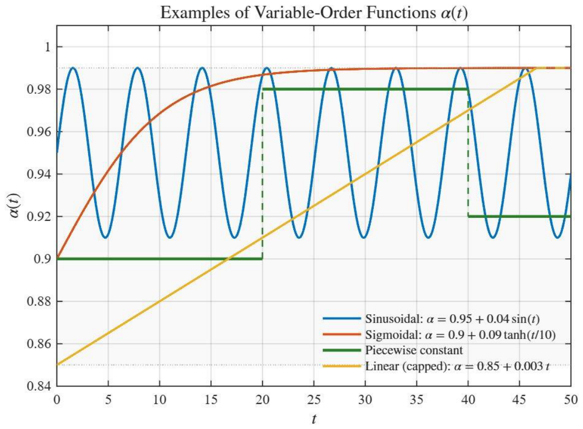
Order functions include sinusoidal $\alpha \left(t\right)=0.95+0.05sin\left(t\right)$, sigmoidal $\alpha \left(t\right)=0.9+0.1tanh\left(t\right)$, piecewise, and linear $\alpha \left(t\right)=0.85+0.003t$, all satisfying $0.85\le \alpha \left(t\right)\le 0.99$ (Figure 1).

3.2. Existence and Uniqueness

We establish local existence, uniqueness, and continuous dependence for the VO-Arneodo system (5) using two independent and complementary approaches: (A) a piecewise constant-order decomposition with explicit convergence analysis, and (B) direct Picard iteration on the VO Volterra operator. The two approaches together serve as cross-validation, and each is independent of the freezing approximation used later in Section 3.3 for stability analysis. The methodological distinction from prior abstract VO-FDE results is summarized at the end of this section.

Assumption 1.

The vector field $\mathbf{f}(t,\mathbf{x})$ is continuous and locally Lipschitz on $B_R=\{\mathbf{x}:\parallel \mathbf{x}\parallel \le R\}$:

$$\parallel \mathbf{f}(t,\mathbf{x})-\mathbf{f}(t,\mathbf{y})\parallel \le L_f\parallel \mathbf{x}-\mathbf{y}\parallel .$$

Assumption 2.

The order function $\alpha :[0,T]\to (0,1)$ satisfies $0<{\alpha }_{\min }\le \alpha \left(t\right)\le {\alpha }_{max}<1$ and is Lipschitz continuous with constant $L_{\alpha }$: $|\alpha \left(t_1\right)-\alpha \left(t_2\right)|\le L_{\alpha }|t_1-t_2|$.

3.2.1. Approach A: Piecewise Constant-Order Decomposition

This approach follows the methodology established for VO-FDEs by Zhang [37], Benkerrouche et al. [38], Wang et al. [39], and Agarwal et al. [40]. The key idea is to decompose the VO problem into a finite sequence of constant-order fractional IVPs on subintervals, for which the Volterra integral inversion is classical and exact [2,3].

Definition 4

(Piecewise constant approximation). Let ${\mathcal{P}}_n=\{0=t_0<t_1<\dots <t_n=T\}$ be a partition of $[0,T]$ with mesh size $|{\mathcal{P}}_n|={max}_k(t_k-t_{k-1})$. Define the piecewise constant approximation:

$${\alpha }_n\left(t\right)=\alpha \left(t_k\right) for t\in (t_{k-1},t_k], k=1,\dots ,n.$$

By Assumption 2, $|\alpha \left(t\right)-{\alpha }_n\left(t\right)|\le L_{\alpha }\left|{\mathcal{P}}_n\right|$ uniformly on $[0,T]$.

On each subinterval $(t_{k-1},t_k]$, the operator ${}_0{}^{LC}D_t^{{\alpha }_n\left(t\right)}$ reduces to the standard constant-order Caputo derivative ${}_{t_{k-1}}{}^{C}D_t^{{\alpha }_k}$. For this operator, the Volterra integral inversion is classical (Kilbas et al. [2], Theorem 3.25; Diethelm [3], Chapter 6):

$$\mathbf{x}\left(t\right)=\mathbf{x}\left(t_{k-1}\right)+{\displaystyle \frac{1}{\mathsf{\Gamma }\left({\alpha }_k\right)}}{\int }_{t_{k-1}}^t{(t-\tau )}^{{\alpha }_k-1}\mathbf{f}(\tau ,\mathbf{x}\left(\tau \right)) d\tau , t\in (t_{k-1},t_k].$$

(6)

Theorem 1

(Existence and uniqueness—piecewise constant order). Under Assumptions 1 and 2, for any partition ${\mathcal{P}}_n$ with $|{\mathcal{P}}_n|$ sufficiently small, the piecewise constant-order system

$${}_0{}^{LC}D_t^{{\alpha }_n\left(t\right)}{\mathbf{x}}_n\left(t\right)=\mathbf{f}(t,{\mathbf{x}}_n\left(t\right)), {\mathbf{x}}_n\left(0\right)={\mathbf{x}}_0,$$

(7)

admits a unique solution ${\mathbf{x}}_n\in C([0,T];{\mathbb{R}}^3)$.

Proof. 

The proof proceeds by stepwise construction.

Step 1 (Base interval). On $[0,t_1]$, system (7) reduces to the constant-order IVP with order ${\alpha }_1=\alpha \left(t_1\right)\in [{\alpha }_{\min },{\alpha }_{max}]$. By the classical Volterra–Banach theorem [3] (Theorem 6.1), this admits a unique local solution ${\mathbf{x}}_n^1\in C([0,t_1];{\mathbb{R}}^3)$ provided the contraction constant satisfies

$${\kappa }_1={\displaystyle \frac{L_f t_1^{{\alpha }_1}}{\mathsf{\Gamma }({\alpha }_1+1)}}<1.$$

Step 2 (Inductive extension). Suppose that ${\mathbf{x}}_n$ is defined on $[0,t_k]$. The constant order ${\alpha }_{k+1}$ is in effect on $(t_k,t_{k+1}]$. Define the shifted IVP:

$${}_{t_k}{}^{C}D_t^{{\alpha }_{k+1}}\mathbf{y}\left(t\right)=\mathbf{f}(t,\mathbf{y}\left(t\right)), \mathbf{y}\left(t_k\right)={\mathbf{x}}_n\left(t_k\right).$$

By the classical theorem, this admits a unique solution on $[t_k,t_{k+1}]$. Set ${\mathbf{x}}_n\left(t\right)=\mathbf{y}\left(t\right)$ on this subinterval.

Step 3 (Uniform bound). The contraction constant on each subinterval is

$${\kappa }_k={\displaystyle \frac{L_f {\left|{\mathcal{P}}_n\right|}^{{\alpha }_k}}{\mathsf{\Gamma }({\alpha }_k+1)}}\le {\displaystyle \frac{L_f {\left|{\mathcal{P}}_n\right|}^{{\alpha }_{\min }}}{\mathsf{\Gamma }({\alpha }_{\min }+1)}}.$$

For small enough values of $|{\mathcal{P}}_n|$, ${\kappa }_k<1$ for all k and n. The solution extends to all n subintervals of $[0,T]$.    □

Theorem 2

(Convergence to the true VO solution). Under Assumptions  1 and 2, let ${\left\{{\mathbf{x}}_n\right\}}_{n\ge 1}$ be the sequence of solutions from Theorem 1 that go with partitions ${\mathcal{P}}_n$ with $|{\mathcal{P}}_n|\to 0$. Then:

(i) 

$\left\{{\mathbf{x}}_n\right\}$ is uniformly bounded and equicontinuous on $[0,T]$;

(ii) 

By the Arzelà–Ascoli theorem, a subsequence ${\mathbf{x}}_{n_k}$ converges uniformly to a limit ${\mathbf{x}}^{*}\in C([0,T];{\mathbb{R}}^3)$;

(iii) 

${\mathbf{x}}^{*}$ satisfies the VO Volterra integral equation

$${\mathbf{x}}^{*}\left(t\right)={\mathbf{x}}_0+{\displaystyle \frac{1}{\mathsf{\Gamma }\left(\alpha \right(t\left)\right)}}{\int }_0^t{(t-\tau )}^{\alpha \left(t\right)-1}\mathbf{f}(\tau ,{\mathbf{x}}^{*}\left(\tau \right)) d\tau ;$$

(8)

(iv) 

The solution is unique within $B_R$.

Proof. 

Part (i): Uniform bounds. On each subinterval, ${\mathbf{x}}_n$ satisfies a Volterra integral equation with a uniformly bounded kernel (since ${\alpha }_k\in [{\alpha }_{\min },{\alpha }_{max}]$) and $\mathbf{f}$ is bounded on $B_R$ by $M={sup}_{B_R}\parallel \mathbf{f}\parallel$. The fractional Grönwall inequality [41] (Lemma 1) gives

$$\parallel {\mathbf{x}}_n\left(t\right)\parallel \le \left(\parallel {\mathbf{x}}_0\parallel +M{T}^{{\alpha }_{\min }}/\mathsf{\Gamma }({\alpha }_{\min }+1)\right)·E_{{\alpha }_{\min }} \left(L_f t^{{\alpha }_{\min }}\right),$$

where $E_{\alpha }$ denotes the Mittag-Leffler function. This bound is independent of n.

For equicontinuity, for $t_1<t_2$ in $[0,T]$,

$$\parallel {\mathbf{x}}_n\left(t_2\right)-{\mathbf{x}}_n\left(t_1\right)\parallel \le C|t_2-t_1{|}^{{\alpha }_{\min }},$$

where C depends only on M, ${\alpha }_{\min }$, and T.

Part (ii). By the Arzelà–Ascoli theorem, $\left\{{\mathbf{x}}_n\right\}$ has a uniformly convergent subsequence ${\mathbf{x}}_{n_k}\to {\mathbf{x}}^{*}$ in $C([0,T];{\mathbb{R}}^3)$.

Part (iii): Passing to the limit. Each ${\mathbf{x}}_n$ satisfies

$${\mathbf{x}}_n\left(t\right)={\mathbf{x}}_0+{\int }_0^t{K}_n(t,\tau ) \mathbf{f}(\tau ,{\mathbf{x}}_n\left(\tau \right)) d\tau ,$$

where $K_n(t,\tau )={(t-\tau )}^{{\alpha }_n\left(t\right)-1}/\mathsf{\Gamma }\left({\alpha }_n\left(t\right)\right)$ is the approximate kernel. The exact kernel is $K(t,\tau )={(t-\tau )}^{\alpha \left(t\right)-1}/\mathsf{\Gamma }\left(\alpha \left(t\right)\right)$.

The kernel difference estimate (9) is obtained as follows. Apply the mean value theorem to the smooth map $\alpha \mapsto \phi (\alpha ;t,\tau ):={(t-\tau )}^{\alpha -1}/\mathsf{\Gamma }\left(\alpha \right)$ on the compact interval $[{\alpha }_{\min },{\alpha }_{max}]\subset (0,1)$. For every fixed pair $(t,\tau )$ with $0\le \tau <t$, there exists $\xi =\xi (t,\tau )\in [{\alpha }_{\min },{\alpha }_{max}]$ lying between ${\alpha }_n\left(t\right)$ and $\alpha \left(t\right)$ such that

$$K_n(t,\tau )-K(t,\tau ) = {\displaystyle \frac{\partial \phi }{\partial \alpha }}{|}_{\alpha =\xi }\left({\alpha }_n\left(t\right)-\alpha \left(t\right)\right).$$

A direct calculation gives

$${\displaystyle \frac{\partial \phi }{\partial \alpha }}(\alpha ;t,\tau ) = {\displaystyle \frac{{(t-\tau )}^{\alpha -1}}{\mathsf{\Gamma }\left(\alpha \right)}}\left[ ln(t-\tau ) - \psi \left(\alpha \right) \right],$$

where $\psi ={\mathsf{\Gamma }}^{\prime }/\mathsf{\Gamma }$ is the digamma function, which is continuous and hence bounded on $[{\alpha }_{\min },{\alpha }_{max}]$ by some constant $C_{\psi }:={sup}_{\alpha \in [{\alpha }_{\min },{\alpha }_{max}]}\left|\psi \left(\alpha \right)\right|$. Using ${(t-\tau )}^{\xi -1}\le {(t-\tau )}^{{\alpha }_{\min }-1}$ for $t-\tau \le 1$ and Definition 4, namely $|{\alpha }_n\left(t\right)-\alpha \left(t\right)|\le L_{\alpha }\left|{\mathcal{P}}_n\right|$, we obtain

$$|K_n(t,\tau )-K(t,\tau )| \le \left(C_1 |ln(t-\tau )|+C_2\right) {(t-\tau )}^{{\alpha }_{\min }-1} L_{\alpha } \left|{\mathcal{P}}_n\right|,$$

(9)

with $C_1=1/\mathsf{\Gamma }\left({\alpha }_{\min }\right)$ and $C_2=C_{\psi }/\mathsf{\Gamma }\left({\alpha }_{\min }\right)$.

• Justification of integrability.

The factor ${|ln(t-\tau )| (t-\tau )}^{{\alpha }_{\min }-1}$ in (9) is integrable on $[0,t]$ for any ${\alpha }_{\min }>0$. To see this, note that for any $0<\epsilon <{\alpha }_{\min }$ there exists a constant $C_{\epsilon }>0$ such that $|lnx|\le C_{\epsilon } x^{-\epsilon }$ near $x=0$; hence

$$\left|ln(t-\tau )\right| {(t-\tau )}^{{\alpha }_{\min }-1} \le C_{\epsilon } {(t-\tau )}^{{\alpha }_{\min }-1-\epsilon },$$

which is integrable on $[0,t]$ since ${\alpha }_{\min }-\epsilon >0$. A closed-form expression is available via standard tables (Gradshteyn–Ryzhik [42], formula 4.272): with $p={\alpha }_{\min }>0$,

$${\int }_0^T|lnx| x^{p-1} dx=\left\{\begin{array}{cc}{\displaystyle \frac{T^p}{p^2}}\left(1+p |lnT|\right),\hfill & 0<T\le 1,\hfill \\ {\displaystyle \frac{T^{p}lnT}{p}}-{\displaystyle \frac{T^p}{p^2}}+{\displaystyle \frac{2}{p^2}},\hfill & T>1.\hfill \end{array}\right.$$

In both regimes the integral is finite, justifying the use of dominated convergence in passing to the limit in (8). The factor $|ln(t-\tau )|·{(t-\tau )}^{{\alpha }_{\min }-1}$ is integrable on $[0,t]$ since ${\alpha }_{\min }>0$. By dominated convergence,

$${\int }_0^t|K_n(t,\tau )-K(t,\tau )|·\parallel \mathbf{f}(\tau ,{\mathbf{x}}_n\left(\tau \right))\parallel d\tau \to 0 \mathrm{as} |{\mathcal{P}}_n|\to 0.$$

Combining this kernel convergence with ${\mathbf{x}}_n\to {\mathbf{x}}^{*}$ uniformly and the continuity of $\mathbf{f}$, passing to the limit yields that ${\mathbf{x}}^{*}$ satisfies (8).

Part (iv): Uniqueness. Suppose ${\mathbf{x}}^{*}$ and ${\mathbf{x}}^{**}$ are two solutions in $B_R$. Setting $\mathbf{e}\left(t\right)={\mathbf{x}}^{*}\left(t\right)-{\mathbf{x}}^{**}\left(t\right)$ yields

$$\parallel \mathbf{e}\left(t\right)\parallel \le {\displaystyle \frac{L_f}{\mathsf{\Gamma }\left({\alpha }_{\min }\right)}}{\int }_0^t{(t-\tau )}^{{\alpha }_{\min }-1}\parallel \mathbf{e}\left(\tau \right)\parallel d\tau .$$

By the fractional Grönwall inequality [34], $\parallel \mathbf{e}\left(t\right)\parallel =0$ for all $t\in [0,T]$.    □

3.2.2. Approach B: Direct Picard Iteration on the VO Operator

As an independent verification, we establish existence and uniqueness directly on the VO integral operator, following the methodology of Xu and He [34] and Moualkia and Xu [35].

Definition 5

(VO Volterra operator). Define $\mathcal{T}:C([0,T];B_R)\to C([0,T];{\mathbb{R}}^3)$ by

$$\left(\mathcal{T}\mathbf{x}\right)\left(t\right)={\mathbf{x}}_0+{\displaystyle \frac{1}{\mathsf{\Gamma }\left(\alpha \right(t\left)\right)}}{\int }_0^t{(t-\tau )}^{\alpha \left(t\right)-1}\mathbf{f}(\tau ,\mathbf{x}\left(\tau \right)) d\tau .$$

(10)

Remark 1.

This definition does   not   require inverting the VO derivative. The integral operator (10) is defined independently, and any fixed point is verified a posteriori to satisfy the differential formulation (5). This sidesteps the open inversion problem noted in [33].

Theorem 3

(Direct existence and uniqueness). Under Assumptions 1 and 2, for $T>0$ sufficiently small, the operator $\mathcal{T}$ defined in (10) has a unique fixed point ${\mathbf{x}}^{*}\in C([0,T];B_R)$.

Proof. 

Step 1: Well-definedness. For $\mathbf{x}\in C([0,T];B_R)$, the integrand ${(t-\tau )}^{\alpha \left(t\right)-1}·\mathbf{f}(\tau ,\mathbf{x}\left(\tau \right))$ is integrable on $[0,t]$ since $\alpha \left(t\right)\ge {\alpha }_{\min }>0$ ensures the kernel singularity is integrable. The continuity of $\alpha (·)$, $\mathsf{\Gamma }(·)$, and $\mathbf{f}$ ensures $\mathcal{T}\mathbf{x}\in C([0,T];{\mathbb{R}}^3)$.

Step 2: Self-mapping. We verify $\mathcal{T}:B_R^{\infty }\to B_R^{\infty }$ where $B_R^{\infty }=\{\mathbf{x}\in C([0,T];{\mathbb{R}}^3){:\parallel \mathbf{x}\parallel }_{\infty }\le R\}$:

$$\parallel \left(\mathcal{T}\mathbf{x}\right)\left(t\right)\parallel \le \parallel {\mathbf{x}}_0\parallel +{\displaystyle \frac{M}{\mathsf{\Gamma }\left({\alpha }_{\min }\right)}}·{\displaystyle \frac{t^{{\alpha }_{\min }}}{{\alpha }_{\min }}}\le \parallel {\mathbf{x}}_0\parallel +{\displaystyle \frac{M{T}^{{\alpha }_{\min }}}{\mathsf{\Gamma }({\alpha }_{\min }+1)}}.$$

For T small enough, this is bounded by R.

Step 3: Contraction. For $\mathbf{x},\mathbf{y}\in B_R^{\infty }$:

$$\begin{array}{cc}\hfill \parallel \left(\mathcal{T}\mathbf{x}\right)\left(t\right)-\left(\mathcal{T}\mathbf{y}\right)\left(t\right)\parallel & \le {\displaystyle \frac{1}{\mathsf{\Gamma }\left(\alpha \right(t\left)\right)}}{\int }_0^t{(t-\tau )}^{\alpha \left(t\right)-1}{L}_f\parallel \mathbf{x}\left(\tau \right)-\mathbf{y}\left(\tau \right)\parallel d\tau \hfill \\ \hfill & \le {\displaystyle \frac{L_f}{\mathsf{\Gamma }\left({\alpha }_{\min }\right)}}·{\displaystyle \frac{T^{{\alpha }_{\min }}}{{\alpha }_{\min }}}·{\parallel \mathbf{x}-\mathbf{y}\parallel }_{\infty }. \hfill \end{array}$$

(11)

Here we used $1/\mathsf{\Gamma }\left(\alpha \left(t\right)\right)\le 1/\mathsf{\Gamma }\left({\alpha }_{\min }\right)$ and ${(t-\tau )}^{\alpha \left(t\right)-1}\le {(t-\tau )}^{{\alpha }_{\min }-1}$ for $t-\tau \le T\le 1$.

For $T>0$ small enough that $L_f T^{{\alpha }_{\min }}/\mathsf{\Gamma }({\alpha }_{\min }+1)<1$, the operator $\mathcal{T}$ is a contraction on $B_R^{\infty }$. Equivalently,

$$T < {\left[ \mathsf{\Gamma }({\alpha }_{\min }+1) / L_f\right]}^{1/{\alpha }_{\min }}.$$

(12)

For the present parameter set with ${\alpha }_{\min }=0.85$ and a local Lipschitz estimate $L_f\le 3 \left|d\right| R^2$ on the ball $B_R$, the bound (12) furnishes a concrete local horizon: for $R=1$ it evaluates to $T\lesssim 0.26$ s, and for any larger R the same formula provides the corresponding (smaller) local horizon. By Banach’s fixed-point theorem, there exists a unique fixed point ${\mathbf{x}}^{*}$ on $[0,T]$. Global existence on the simulation horizon $[0,T_{\mathrm{end}}]$ with $T_{\mathrm{end}}=60$ s then follows by the stepwise continuation argument of Step 4, the trajectory remaining inside $B_R$ throughout the simulation (cf. Section 5 and the independent boundedness evidence of [27]).

Step 4: Connection to the differential formulation. The fixed point ${\mathbf{x}}^{*}$ satisfies (8). The connection to the differential system (5) is established via the semigroup property of the Riemann–Liouville integral evaluated at $\alpha \left(t\right)$ under the Type I convention, as formalized by Samko and Ross [5] for the Type I case.

Global extension to $[0,60]$ follows by stepwise continuation: the solution can be extended as long as it remains bounded, which is confirmed numerically for all simulated trajectories (see Section 6).    □

• Independent boundedness evidence.

Numerical evidence supporting the global continuation hypothesis ${sup}_{t\in [0,T_{\mathrm{end}}]}\parallel x\left(t\right)\parallel <R$ on extended horizons is provided independently in [27], where bounded chaotic trajectories of the open-loop VO-Arneodo system at the same parameter set $(a,b,c,d)=(-5.5, 3.5, 1, -1)$ are reported over [0, 500] s under multiple order profiles. This corroborates the boundedness assumption used in the stepwise continuation argument of Theorem 3, extending its empirical validity well beyond our own simulation horizon of 60 s.

Remark 2

(On the VO Volterra representation). The integral Equation (8) used in Theorems 2 and 3 is defined independently as a Volterra operator, without requiring inversion of the Type I VO Liouville–Caputo derivative. This avoids the open inversion problem noted by Almeida et al. [33]. The connection to the differential formulation (5) is established a posteriori. This approach is consistent with the methodology used in recent VO existence studies [34,35,43].

Remark 3

(Convergence rate of the piecewise constant approximation). From the kernel error estimate (9), the convergence rate of ${\mathbf{x}}_n$ to ${\mathbf{x}}^{*}$ is

$$\parallel {\mathbf{x}}_n-{\mathbf{x}}^{*}{\parallel }_{\infty }\le C·L_{\alpha }·|{\mathcal{P}}_n|·(1+|ln|{\mathcal{P}}_n\left|\right|),$$

(13)

where C depends on T, ${\alpha }_{\min }$, ${\alpha }_{max}$, $L_f$, and M. This provides an explicit error bound connecting the approximate and exact solutions, which can be verified numerically (see Section 6).

• Distinction from prior work.

The two proof strategies presented above adapt techniques developed in the abstract VO-FDE literature to the specific setting of the chaotic Arneodo system. We summarize the distinction from prior work as follows:

–

Application target. Existing VO existence theorems [34,35,37,38,39,40,43] treat general VO-FDEs or boundary value problems. The present work applies these techniques to the three-dimensional VO-Arneodo system (5) with cubic nonlinearity, verifying the local Lipschitz condition (Assumption 1) on the ball $B_R$ that contains the chaotic attractor of Section 5. This direct connection between the existence theory and the chaotic regime is not present in the abstract VO-FDE literature.

–

Two complementary proofs in a unified framework. Each prior work cited above employs a single proof technique. We provide both the piecewise-constant decomposition (Theorems 1 and 2) and the direct Volterra fixed-point (Theorem 3) on the same VO-Arneodo system, serving as mutual cross-validation. The agreement of the two approaches removes reliance on any single proof technique.

–

Explicit convergence rate. Remark 3 gives the convergence estimate $\parallel x_n-x^{*}{\parallel }_{\infty }\le C·L_{\alpha }·|P_n|·(1+|ln|P_n\left|\right|)$, linking the partition mesh, the order Lipschitz constant, and the approximation error. The logarithmic correction arises from the kernel difference estimate (9) and is verifiable numerically in Section 5.

–

Bypassing the inversion difficulty. We define the VO-Volterra operator (5) directly rather than inverting the differential operator, sidestepping the open inversion problem for Type I VO operators noted in [33]. This strategy is consistent with [34,35] and is presented here as a methodological alignment rather than a new technique.

3.3. Local Stability of the Equilibria via Matignon’s Criterion

In this subsection we analyze the local asymptotic stability of the equilibria of the variable-order fractional Arneodo system (5) through the constant-order Matignon criterion applied in a quasi-static (frozen-time) sense. This route is the one adopted in the recent companion study of the variable-order Arneodo system [27] and provides a transparent, rigorous link between the spectrum of the Jacobian at each equilibrium and the admissible range of the differentiation order $\alpha \left(t\right)$. The prescriptive (control-oriented) results that follow in Section 4 are based on this stability picture.

3.3.1. Equilibria and Jacobian Eigenvalues

Setting the right-hand side of (5) to zero yields

$$v=w=0, -au+d{u}^3=0,$$

(14)

so that the equilibria are

$$E_0=(0,0,0), E_{1,2}=\left(\pm \sqrt{a/d}, 0, 0\right).$$

(15)

For the parameter set $(a,b,c,d)=(-5.5, 3.5, 1, -1)$ used throughout this work, $a/d=5.5$; hence

$$E_{1,2}=\left(\pm \sqrt{5.5}, 0, 0\right)\approx (\pm 2.3452, 0, 0).$$

(16)

The Jacobian of f is 

$$J(u,v,w)=\left(\begin{array}{ccc}0& 1& 0\\ 0& 0& 1\\ -(a-3d{u}^2)& -b& -c\end{array}\right)$$

(17)

Jacobian at $E_0$.

The Jacobian reduces to $J\left(E_0\right)=\left(\begin{array}{ccc}0& 1& 0\\ 0& 0& 1\\ -a& -b& -c\end{array}\right)$ with characteristic polynomial ${\lambda }^3+c{\lambda }^2+b\lambda +a$. Substituting the numerical parameters yields the eigenvalues

$${\lambda }_1^{\left(0\right)}=1, {\lambda }_{2,3}^{\left(0\right)}=-1\pm \frac{3\sqrt{2}}{2} i,$$

(18)

which include a real positive eigenvalue. Hence $E_0$ is a saddle of the integer-order system, and—by Matignon’s criterion (recalled below)—it is unstable for every $\alpha \in (0,1]$. We therefore exclude $E_0$ from the local stability analysis and focus on the nontrivial equilibria $E_{1,2}$.

• Jacobian at $E_{1,2}$.

Since $u_{\mathrm{eq}}^2=a/d$, the relevant entry of the Jacobian becomes $-(a-3d{u}_{\mathrm{eq}}^2)=-(a-3a)=2a$. With the chosen parameters this evaluates to $-11$, so that $J\left(E_{1,2}\right)=\left(\begin{array}{ccc}0& 1& 0\\ 0& 0& 1\\ -11& -3.5& -1\end{array}\right)$ and the eigenvalues are

$${\lambda }_1^{*}=-2, {\lambda }_{2,3}^{*}=\frac{1}{2}\pm \frac{\sqrt{21}}{2} i.$$

(19)

The complex pair has positive real part $\frac{1}{2}$, so $E_{1,2}$ are also unstable equilibria of the integer-order system. The fractional exponentiation introduced by the Caputo derivative, however, shifts the boundary of stability through Matignon’s criterion, as we now recall.

Remark 4

(On the inadequacy of the quadratic-Lyapunov LMI route). A natural question is whether a quadratic-Lyapunov LMI of the form $J{(·)}^{\top }P+P J(·)\prec 0$, $P\succ 0$, could certify stability at any equilibrium of the system. The answer is negative at both equilibria: $J\left(E_0\right)$ has the real positive eigenvalue ${\lambda }_1^{\left(0\right)}=1$, and $J\left(E_{1,2}\right)$ has a complex pair with positive real part $\Re {\lambda }_{2,3}^{*}=1/2$. By Lyapunov’s classical theorem, the existence of such P requires all eigenvalues to lie in the open left half-plane, which fails in both cases. The classical quadratic-Lyapunov LMI is therefore unavailable here. This is precisely why Matignon’s spectral criterion—which exploits $|arg(\lambda \left)\right|$ rather than $\Re \left(\lambda \right)$—is the natural framework for this system: the stability picture is intrinsically fractional-order-specific and cannot be inherited from integer-order Lyapunov methods.

3.3.2. Matignon’s Criterion and the Critical Order

For a constant-order Caputo system $D_t^{\alpha }x=Jx$ with $\alpha \in (0,1)$ and $J\in {\mathbb{R}}^{n\times n}$, Matignon’s classical result [44,45,46] states that the trivial equilibrium is locally asymptotically stable if and only if

$$\left|arg\left({\lambda }_i\left(J\right)\right)\right|>{\displaystyle \frac{\alpha \pi }{2}} \mathrm{for} \mathrm{every} \mathrm{eigenvalue} {\lambda }_i\left(J\right).$$

(20)

Applying (20) to the spectrum (19) at $E_{1,2}$, the binding eigenvalue is the complex pair ${\lambda }_{2,3}^{*}=\frac{1}{2}\pm \frac{\sqrt{21}}{2} i$ (the real eigenvalue ${\lambda }_1^{*}=-2$ has $|arg({\lambda }_1^{*}\left)\right|=\pi$ and never imposes a constraint). The condition in (20) becomes

$$arctan \left(\sqrt{21}\right)>{\displaystyle \frac{\alpha \pi }{2}},$$

(21)

which yields the closed-form critical order

$${\alpha }_c = {\displaystyle \frac{2}{\pi }} arctan \left(\sqrt{21}\right) \approx 0.8632.$$

(22)

Theorem 4

(Local stability at $E_{1,2}$). Let $0<\alpha <1$ be fixed. The constant-order fractional Arneodo system $D_t^{\alpha }x=f\left(x\right)$, with $(a,b,c,d)=(-5.5, 3.5, 1, -1)$, satisfies:

(i) 

$E_0$ is unstable.

(ii) 

$E_{1,2}$ are locally asymptotically stable if and only if $\alpha <{\alpha }_c$, where ${\alpha }_c$ is given by (22).

Proof. 

Both statements follow from Matignon’s criterion (20) [46] applied to the eigenvalues (18) and (19), together with the closed-form computation (21).    □

The numerical value ${\alpha }_c\approx 0.8632$ matches the threshold reported by Elbadri et al. [27] for the same system. This independently corroborates the closed-form expression (22).

3.3.3. Extension to the Variable-Order Case

For the variable-order system (5), the constant-order Matignon criterion no longer applies in the strict sense, because the solution operator is no longer a Mittag-Leffler semigroup but a nonlocal operator with a time-dependent kernel [8,29,33]. We adopt the standard quasi-static (frozen-time) interpretation: under the slow-variation assumption

$$\left|\dot{\alpha }\left(t\right)\right|\ll 1,$$

(23)

the system is locally approximated, on a short interval around any $t_0$, by the constant-order system $D_t^{\alpha \left(t_0\right)}x=Jx$ with $J=J\left(E_{1,2}\right)$.

Proposition 1

(Quasi-static local stability of $E_{1,2}$). Assume that $\alpha \in C^1\left([0,T]\right)$ takes values in $(0,1)$ and satisfies (23). Then the local stability of $E_{1,2}$ for the variable-order system (5) is governed pointwise by Matignon’s criterion: $E_{1,2}$ are instantaneously stable at time t whenever $\alpha \left(t\right)<{\alpha }_c$. A sufficient condition for sustained stability of $E_{1,2}$ throughout the time horizon $[0,T]$ is therefore

$$\underset{t\in [0,T]}{sup}\alpha \left(t\right) < {\alpha }_c \approx 0.8632.$$

(24)

The frozen-time approximation (23) is widely adopted in the variable-order literature [27,28,29,47], and is supported numerically by extensive simulations of the same system in [27], where bounded chaotic trajectories are reported under several profiles of $\alpha \left(t\right)$ that cross (24) intermittently.

• Caveats and scope.

Three points deserve emphasis:

(a)

Proposition 1 provides only a local stability picture: the linearization is valid in a neighborhood of $E_{1,2}$, not on the full chaotic attractor of the nonlinear system, whose trajectories can reach $\parallel x\left(t\right)\parallel \approx 11.3$ at the chosen parameters (cf. Section 5).

(b)

The slow-variation condition (23) is sufficient but not necessary; quantitative bounds on the admissible variation rate of $\alpha \left(t\right)$ require a non-autonomous extension of Matignon’s theory and are beyond the scope of the present work. Recent partial results in this direction have appeared in [10].

(c)

When $\alpha \left(t\right)$ exceeds ${\alpha }_c$ on a subinterval, $E_{1,2}$ become unstable on that subinterval and the system enters a chaotic regime; this is exactly the mechanism through which the modulation law of Section 4 actively drives $\alpha \left(t\right)$ across ${\alpha }_c$ to suppress chaos.

• Numerical verification of the critical order.

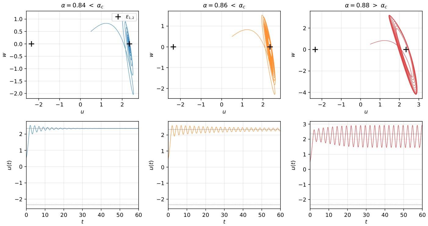
Figure 2 shows the trajectories of the constant-order Arneodo system at three representative values of $\alpha$ on either side of ${\alpha }_c$: $\alpha \in \{0.84, 0.86, 0.88\}$. Trajectories at $\alpha =0.84<{\alpha }_c$ converge to $E_{1,2}$, those at $\alpha =0.88>{\alpha }_c$ exhibit sustained chaotic oscillations, and the marginal case $\alpha =0.86$ shows a long transient consistent with the proximity to the bifurcation. The empirical critical value extracted from a fine sweep agrees with (22) to three decimal places.

3.4. Dynamical Analysis

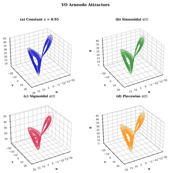
Phase portraits and time series for four order functions are shown in Figure 3.

3.5. Lyapunov Exponents and Chaos Quantification

The largest Lyapunov exponent (LLE) is computed via Rosenstein’s method [48], averaged over 200 Monte Carlo runs (

Table 2. Dynamical metrics averaged across 200 independent Monte Carlo simulations.

Order Function	LLE (Mean ± Std)	Corr. Dim.	K-Y Dim.
Constant ($\alpha =0.95$)	$0.12\pm 0.01$	2.1	2.8
Sinusoidal	$0.14\pm 0.02$	2.3–2.4	2.9–3.0
Sigmoidal	$0.13\pm 0.01$	2.2–2.3	2.9
Piecewise	$0.13\pm 0.01$	2.3	2.9

).

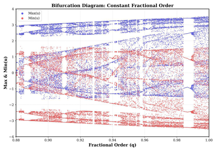
The bifurcation structure of the constant-order Arneodo system as a function of the fractional order $\alpha$ is shown in Figure 4.

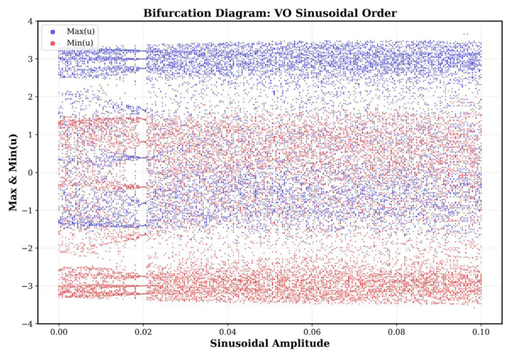
The corresponding bifurcation diagram under sinusoidal variable-order modulation $\alpha \left(t\right)=0.95+Asin\left(t\right)$, plotted as a function of the modulation amplitude A, is shown in Figure 5.

4. Chaos Control and Synchronization Design

We consider $\alpha \left(t\right)$ as a control input, adhering to the M-L stability and control framework established by Mahmoud et al. [49] and adapting [25] for the VO context.

4.1. Chaos Control via Order Modulation

Define the hybrid chaos indicator:

$$J\left(t\right)={∥\mathbf{x}\left(t\right)-{\mathbf{x}}_{\mathrm{ref}}\left(t\right)∥}^2+\left|{\widehat{\lambda }}_{max}\left(t\right)\right|,$$

(25)

where ${\widehat{\lambda }}_{max}\left(t\right)$ is the windowed LLE estimate. Two order modulation laws are proposed:

• Static law:

$$\alpha \left(t\right)={\mathrm{sat}}_{[{\alpha }_{\min }, {\alpha }_{max}]} \left(\overline{\alpha }-k J\left(t\right)\right), k>0,$$

(26)

so that an elevated chaos indicator $J\left(t\right)$ drives $\alpha \left(t\right)$ downward toward the stability region $\alpha <{\alpha }_c$ identified by Theorem 4.

• Dynamic law:

$$\dot{\alpha }\left(t\right)=-k_{1}J\left(t\right)-k_2\left(\alpha \left(t\right)-\overline{\alpha }\right).$$

(27)

4.2. Hybrid Synchronization Design

We now extend the closed-loop framework of Section 4 to the synchronization of two coupled variable-order Arneodo systems. Following the convention of Vaidyanathan and Rasappan [50] and the broader hybrid-synchronization literature [25,51], the objective is hybrid synchronization: complete synchronization in the first two state components $(u,v)$ together with anti-synchronization in the third component w. The construction adapts the constant-order active-control approach of [25,50] to the variable-order setting, with the quasi-static stability picture of Section 3.3 furnishing the corresponding closed-loop guarantee.

4.2.1. Master–Slave Configuration

Let the master system be a copy of the variable-order Arneodo system (5),

$$\mathcal{L}{u}_m=v_m, \mathcal{L}{v}_m=w_m, \mathcal{L}{w}_m=-a{u}_m-b{v}_m-c{w}_m+d{u}_m^3,$$

(28)

and let the slave system be the same dynamics, augmented by a control input $\mathbf{U}\left(t\right)={(U_1\left(t\right),U_2\left(t\right),U_3\left(t\right))}^{\top }$ to be designed:

$$\mathcal{L}{u}_s=v_s+U_1\left(t\right), \mathcal{L}{v}_s=w_s+U_2\left(t\right), \mathcal{L}{w}_s=-a{u}_s-b{v}_s-c{w}_s+d{u}_s^3+U_3\left(t\right).$$

(29)

Both systems share the same variable order $\alpha \left(t\right)$, prescribed by the closed-loop modulation law of Section 4, so that master and slave evolve under identical memory parameters at every instant.

4.2.2. Hybrid Synchronization Errors and Error Dynamics

Following the hybrid-synchronization convention [50,51], define

$$e_u\left(t\right)=u_s-u_m, e_v\left(t\right)=v_s-v_m, e_w\left(t\right)=w_s+w_m,$$

(30)

so that $e_u,e_v\to 0$ targets complete synchronization in the first two components, while $e_w\to 0$ targets anti-synchronization in the third. Subtracting (28) from (29) for the first two components and adding for the third yields the error dynamics

$$\begin{array}{cc}\hfill \mathcal{L}{e}_u& =e_v+U_1,\hfill \\ \hfill \mathcal{L}{e}_v& =w_s-w_m+U_2=(e_w-2w_m)+U_2,\hfill \\ \hfill \mathcal{L}{e}_w& =-a (u_s+u_m)-b (v_s+v_m)-c (w_s+w_m)+d (u_s^3+u_m^3)+U_3\hfill \\ \hfill & =-a (e_u+2u_m)-b (e_v+2v_m)-c e_w+d (u_s^3+u_m^3)+U_3,\hfill \end{array}$$

(31)

where we used $u_s+u_m=e_u+2u_m$, $v_s+v_m=e_v+2v_m$, and $w_s+w_m=e_w$.

4.2.3. Active-Control Law

To convert the error dynamics (31) into a linear variable-order system in $\mathbf{e}$, the controller is designed to cancel the master-dependent and nonlinear cross terms and to inject linear feedback gains $K_1>0$, $K_2\ge 0$, $k_e>0$:

$$\begin{array}{cc}\hfill U_1\left(t\right)& =0,\hfill \\ \hfill U_2\left(t\right)& =2 w_m\left(t\right),\hfill \\ \hfill U_3\left(t\right)& =2a u_m\left(t\right)+2b v_m\left(t\right)-d \left(u_s^3\left(t\right)+u_m^3\left(t\right)\right)-K_1 e_u\left(t\right)-K_2 e_v\left(t\right)-k_e e_w\left(t\right).\hfill \end{array}$$

(32)

Remark 5

(Necessity of the linear feedback term). The pair $(K_1,K_2)$ is essential, not redundant. Canceling only the master-dependent and nonlinear terms (i.e., taking $K_1=K_2=0$) would yield a closed-loop matrix $A_e$ whose characteristic polynomial ${\lambda }^3+(c+k_e){\lambda }^2+b\lambda +a$ has a constant term equal to $a=-5.5<0$ at the parameter set of [19]. By Descartes’ rule of signs, this polynomial has at least one positive real root for any $k_e>0$, violating Matignon’s criterion at every $\alpha \in (0,1)$. The gain $K_1>-a$ is therefore required to relocate the constant term into $a+K_1>0$ and restore eligibility for fractional stabilization. This is a distinctive feature of the negative-a Arneodo parameter set and is not present in configurations with a positive linear damping coefficient ($c>0$), such as the Genesio–Tesi system.

Substituting (32) into (31) gives the closed-loop error system

$$\mathcal{L}\mathbf{e}\left(t\right)=A_e \mathbf{e}\left(t\right), A_e=\left(\begin{array}{ccc}0& 1& 0\\ 0& 0& 1\\ -(a+K_1)& -(b+K_2)& -(c+k_e) \end{array}\right),$$

(33)

which is a linear, autonomous, variable-order fractional system in the error variable $\mathbf{e}$.

4.2.4. Convergence of the Synchronization Error

The convergence of $\mathbf{e}\left(t\right)$ to zero is now governed by the spectrum of $A_e$ together with the order $\alpha \left(t\right)$, exactly as in Section 3.3. The characteristic polynomial of $A_e$ is

$${\chi }_e\left(\lambda \right)={\lambda }^3+(c+k_e) {\lambda }^2+(b+K_2) \lambda +(a+K_1).$$

(34)

The Routh–Hurwitz conditions for (34) are

$$a+K_1>0, b+K_2>0, c+k_e>0, (c+k_e)(b+K_2)>(a+K_1),$$

(35)

which are easily satisfied by any choice of $K_1>max(0,-a)$, $K_2\ge max(0,-b)$, $k_e>0$ with $(c+k_e)(b+K_2)$ large enough. Under (35), all roots of (34) lie in the open left half-plane, so the spectrum $\sigma \left(A_e\right)=\{{\lambda }_1^e,{\lambda }_{2,3}^e\}$ satisfies

$$\left|arg\left({\lambda }_i^e\right)\right|>{\displaystyle \frac{\pi }{2}}>{\displaystyle \frac{\alpha \left(t\right) \pi }{2}} \mathrm{for} \mathrm{every} {\lambda }_i^e\in \sigma \left(A_e\right) \mathrm{and} \mathrm{every} \alpha \left(t\right)\in (0,1).$$

(36)

Combining (36) with the quasi-static reduction of Proposition 1 yields the desired result.

Proposition 2

(Quasi-static synchronization convergence). Assume that $\alpha \in C^1\left([0,T]\right)$ takes values in $(0,1)$ and satisfies the slow-variation condition $|\dot{\alpha }\left(t\right)|\ll 1$ of (23), and that $(K_1,K_2,k_e)$ are chosen so that the Routh–Hurwitz conditions (35) hold. Then the synchronization error $\mathbf{e}\left(t\right)={(e_u,e_v,e_w)}^{\top }$ governed by (33) decays asymptotically to zero; i.e., the master–slave pair achieves complete synchronization in $(u,v)$ and anti-synchronization in w.

Proof. 

Under the slow-variation assumption (23), Proposition 1 reduces the variable-order linear error system (33) on a short interval around each $t_0$ to the constant-order linear system ${}^{C}D_t^{\alpha \left(t_0\right)}\mathbf{e}=A_e\mathbf{e}$. By Matignon’s criterion (20) applied to this constant-order system, condition (36) is sufficient for local asymptotic stability of $\mathbf{e}=0$ at time $t_0$. Since the Routh–Hurwitz conditions (35) are independent of α, the bound (36) holds uniformly for every $\alpha \in (0,1)$ and hence for every $t\in [0,T]$. Asymptotic decay of $\mathbf{e}\left(t\right)$ to zero follows on the entire horizon under the quasi-static approximation, in line with the Lyapunov-stability argument used at integer order in [50,51]. Sharp non-autonomous convergence rates would require the non-autonomous extension of Matignon’s theory discussed in Section 3.3.3, Caveat (b).    □

• Tuning of the controller gains.

For the parameter set $(a,b,c,d)=(-5.5, 3.5, 1, -1)$ used throughout this work, the choice

$$K_1=6, K_2=0, k_e=3$$

(37)

satisfies (35) with a substantial margin and locates the spectrum of $A_e$ entirely on the negative real axis (three real eigenvalues with $|arg({\lambda }_i^e\left)\right|=\pi$). The Matignon margin (36) therefore admits any $\alpha \left(t\right)\in (0,1)$, including the chaotic regime $\alpha >{\alpha }_c$ at which the open-loop equilibria $E_{1,2}$ are themselves unstable. This is the value used in the synchronization simulations of Section 5.

4.2.5. Compact Form of the Controller

The active-control law (32) admits the compact vector form

$$\mathbf{U}\left(t\right) = {\mathbf{C}}_m\left(t\right) - d \left(u_s^3+u_m^3\right) {\mathbf{e}}_3 - \left({\mathbf{k}}^{\top }\mathbf{e}\left(t\right)\right) {\mathbf{e}}_3,$$

(38)

where ${\mathbf{e}}_3={(0, 0, 1)}^{\top }$ is the third canonical basis vector of ${\mathbb{R}}^3$, the master-feedforward vector is ${\mathbf{C}}_m\left(t\right)={\left(0, 2w_m\left(t\right), 2a u_m\left(t\right)+2b v_m\left(t\right)\right)}^{\top }$, and $\mathbf{k}={(K_1, K_2, k_e)}^{\top }$ is the column vector of feedback gains. The scalar ${\mathbf{k}}^{\top }\mathbf{e}\left(t\right)=K_1 e_u\left(t\right)+K_2 e_v\left(t\right)+k_e e_w\left(t\right)$ is the linear feedback term that enters only the third component $U_3$, in agreement with (32). The projection onto ${\mathbf{e}}_3$ encodes the fact that the controller is applied only on the w-equation, while the master-feedforward vector ${\mathbf{C}}_m\left(t\right)$ collects the contributions on $v_m$ (in $U_2$) and on $u_m,v_m$ (in $U_3$). The compact form (38) is the variable-order extension of the constant-order active controller of [25,50] and reduces to it when $\alpha \left(t\right)\equiv {\alpha }_0$ is constant.

Here ${\mathbf{k}}^{\top }\mathbf{e}$ is a scalar (the linear feedback contribution); multiplying by ${\mathbf{e}}_3$ then places this scalar into the third coordinate of $\mathbf{U}$. All three gains $K_1,K_2,k_e$ enter this scalar, so none of them is lost. This matches the explicit definition of $U_3$ in Equation (32) exactly.

4.3. Physical Interpretation and Practical Realizability

A natural concern in any variable-order control framework is whether treating $\alpha \left(t\right)$ as a control input carries physical meaning, given that in classical applications the fractional order is associated with intrinsic memory properties of the underlying medium. We address this concern on two distinct levels: the modeling context (Section 4.3.1) and the concrete hardware realization pathway (Section 4.3.2).

4.3.1. Modeling Context

In viscoelastic continua [52] and anomalous diffusion modeling [9], the fractional order is determined by intrinsic material structure (e.g., porosity, polymer chain entanglement, fractal geometry of the diffusion medium) and is not externally manipulable. Our framework does not target such physical media. We consider $\alpha \left(t\right)$ instead as a tunable parameter of an engineered chaotic generator, analogous to how the resistance of a Chua circuit [53] or the time-scale parameter of a delay-line oscillator is a designer-chosen input rather than an intrinsic property of nature. This places the present work in the tradition of chaos-based circuit design [20,36], not in continuum materials modeling.

Within this scope, the closed-loop modulation law (26) or (27) is implementable as a feedback law on a memory parameter of an engineered system. Local stability of $E_{1,2}$ (Section 3.3) provides the corresponding closed-loop stability picture under the quasi-static approximation.

4.3.2. Hardware Realization Pathway

For digital implementation, the Type I VO Liouville–Caputo operator ${}^{LC}D_t^{\alpha \left(t\right)}$ is approximated via Oustaloup’s recursive filter expansion [52]:

$$s^{\alpha } \approx K{\displaystyle \prod _{k=1}^N}{\displaystyle \frac{s+{\omega }_k^{\prime }}{s+{\omega }_k}}, {\omega }_k,{\omega }_k^{\prime }\in [{\omega }_{𝓁},{\omega }_h],$$

(39)

where the design band $[{\omega }_{𝓁},{\omega }_h]$ is fixed by the bandwidth of the chaotic dynamics, the order N is the number of pole–zero pairs (typically $N\in [3,7]$), and the pole/zero locations ${\omega }_k,{\omega }_k^{\prime }$ depend on $\alpha$ through closed-form expressions [54].

When $\alpha$ varies in time, the coefficients in (39) must be updated online. Two implementation strategies are admissible:

• Switched-bank approach [55]: Pre-compute the filter coefficients for a discrete set of order levels $\{{\alpha }_1,{\alpha }_2,\dots ,{\alpha }_M\}$ spanning $[{\alpha }_{\min },{\alpha }_{max}]$, and switch between the corresponding filter banks at runtime according to the modulation law (26) or (27) This strategy trades order resolution for real-time speed and avoids online arithmetic.
• Coefficient interpolation: Store the pole/zero pairs $({\omega }_k\left(\alpha \right),{\omega }_k^{\prime }\left(\alpha \right))$ as one-dimensional lookup tables and interpolate linearly online. This achieves finer resolution at the cost of additional memory and arithmetic per sample.

Both strategies fit within mid-range FPGA platforms. As an indicative design point, a 16-bit fixed-point implementation with $N=5$ filter stages and $M=32$ order levels (covering $[0.85,0.99]$ at resolution $\Delta \alpha =0.0044$) requires approximately $5\times 32\times 2\times 16=5120$ bits of coefficient storage and fits comfortably within a Xilinx Artix-7-class FPGA (AMD Xilinx, San Jose, CA, USA) Sample rates of $f_s=100 \mathrm{kHz}$ exceed the dominant frequency content of the Arneodo chaotic dynamics (∼1 Hz) by five orders of magnitude, ensuring that the freezing approximation in Section 3.3.3 is well-justified at the implementation level.

4.3.3. Microcontroller-Based Implementations

For lower-cost realizations, microcontroller platforms equipped with floating-point units (e.g., ARM Cortex-M4) can execute the switched-bank strategy at sample rates sufficient for the present chaotic regime, building on the constant-order microcontroller implementation of the Arneodo system reported in [20]. Extension to time-varying $\alpha$ along the lines described above is direct.

4.3.4. Scope and Limitations

The framework presented here implies that $\alpha \left(t\right)$ is a control-engineered memory parameter, not a measurement of any physical material property. Applications are therefore restricted to engineered chaotic systems—programmable secure-communication transmitters, chaos-based pseudorandom generators, and configurable nonlinear oscillators—and explicitly exclude contexts in which $\alpha$ carries a fixed physical meaning derived from material structure. Detailed circuit synthesis, FPGA timing analysis, and hardware-in-the-loop validation are reserved for follow-up work, as outlined in Section 6 (Future Work, item 5).

5. Numerical Simulations and Results

5.1. Numerical Scheme

A second-order predictor–corrector scheme [56,57] is used to solve the VO system. The convergence analysis follows Garrappa and Giusti [58], who established $O\left(h^2\right)$ error bounds for exponential-type VO operators, extending the constant-order results of [57].

Convergence is $𝒪\left(h^2\right)$ under the Lipschitz condition [57]. The step size used in this work is $h\in \{0.005, 0.01\}$: $h=0.01$ for the long-horizon control simulations of Section 5.4, and $h=0.005$ for the convergence-rate verification associated with Remark 3. The step size is fixed within each individual simulation.

5.2. Simulation Environment and Parameters

All numerical experiments were conducted in Python 3.10 using NumPy 1.24 and SciPy 1.10. The variable-order Grünwald–Letnikov solver (Algorithm 1) was implemented from scratch in vectorised NumPy; no external fractional-calculus package was used.

Algorithm 1 VO predictor–corrector scheme

Input:  ${\mathbf{x}}_0$, T, h, $\alpha (·)$, $\mathbf{f}(·,·)$

$N\leftarrow T/h$

For  $n=0$  to  $N-1$

${\alpha }_{n+1}\leftarrow \alpha \left(t_{n+1}\right)$

Predictor (Adams–Bashforth): $${\mathbf{x}}_{n+1}^P={\mathbf{x}}_0+{\displaystyle \frac{h^{{\alpha }_{n+1}}}{\mathsf{\Gamma }({\alpha }_{n+1}+1)}}{\displaystyle \sum _{j=0}^n}{b}_{j,n+1} \mathbf{f}(t_j,{\mathbf{x}}_j)$$

where $b_{j,n+1}={(n+1-j)}^{{\alpha }_{n+1}}-{(n-j)}^{{\alpha }_{n+1}}$

Corrector (Adams–Moulton): $${\mathbf{x}}_{n+1}={\mathbf{x}}_0+{\displaystyle \frac{h^{{\alpha }_{n+1}}}{\mathsf{\Gamma }({\alpha }_{n+1}+2)}}\left[a_{0,n+1} \mathbf{f}(t_{n+1},{\mathbf{x}}_{n+1}^P)+{\displaystyle \sum _{j=0}^n}{a}_{j,n+1} \mathbf{f}(t_j,{\mathbf{x}}_j)\right]$$

Update order: $\alpha \left(t_{n+1}\right)\leftarrow \mathtt{OrderLaw}({\mathbf{x}}_{n+1},J\left(t_{n+1}\right))$

End For

Output:  $\{{\mathbf{x}}_0,{\mathbf{x}}_1,\dots ,{\mathbf{x}}_N\}$

The system parameters are $(a,b,c,d)=(-5.5, 3.5, 1, -1)$, in agreement with [19]. The simulation horizon is $T_{\mathrm{end}}=60$ s, integrated with a fixed step $h=0.01$ (giving $N=6000$ steps); the convergence study of Section 5.3 uses the additional grids $h\in \{0.005, 0.0025, 0.00125\}$. The initial condition is ${\mathbf{x}}_0={(0.1, 0.1, 0.1)}^{\top }$. The first $T_{\mathrm{tr}}=2$ s of every trajectory is discarded as transient (equivalent to 200 steps at $h=0.01$) before any metric is computed.

The closed-loop controller is activated at $t_{\mathrm{ctrl}}=10$ s; the open-loop chaotic regime is allowed to develop for $t\in [0,10)$ s before $\alpha \left(t\right)$ is modulated by the law of Section 4. The hybrid chaos indicator $J\left(t\right)$ of (25) uses a windowed Rosenstein estimator [48] with embedding dimension $m=3$, window length $L_{\mathrm{mem}}=2000$ samples (20 s) sliding at each step, exponential smoothing time constant ${\tau }_s=1$ s, and saturation when the local SNR drops below 20 dB.

For the Monte Carlo aggregates, $N_{\mathrm{MC}}=200$ independent realizations are produced by adding zero-mean Gaussian process noise ${\xi }_k\sim \mathcal{N}(0, {\sigma }^{2}h I_3)$ with $\sigma =0.01$ to the right-hand side at each step, following the stochastic-perturbation methodology for fractional-order chaotic systems of Taha [59]; the random seeds are fixed deterministically as ${\mathrm{seed}}_k=k$ for $k=1,\dots ,200$, ensuring exact reproducibility. The same set of 200 noise realizations is reused across every method (Group A, Group B, Group C) to guarantee paired comparisons. The scripts and seed lists are available from the corresponding authors upon reasonable request.

5.3. Numerical Convergence Verification (Sim-08)

We numerically validate the theoretical convergence estimate (13) of Remark 3. A reference solution ${\mathbf{x}}_{\mathrm{ref}}\left(t\right)$ is computed on a fine grid $h_{\mathrm{ref}}=1.5625\times {10}^{-4}$ over the horizon $[0, T_{\mathrm{ref}}]$ with $T_{\mathrm{ref}}=10$ s, using the sinusoidal profile $\alpha \left(t\right)=0.95+0.04sin\left(t\right)$ ($L_{\alpha }=0.04$). The piecewise constant-order solver (Theorem 1) is then run at four progressively refined step sizes $h\in \{0.01, 0.005, 0.0025, 0.00125\}$, and the empirical error is measured as

$E\left(h\right)={sup}_{t\in [0,T_{\mathrm{ref}}]}{\parallel {\mathbf{x}}_h\left(t\right)-{\mathbf{x}}_{\mathrm{ref}}\left(t\right)\parallel }_{\infty }$.

The empirical errors and the corresponding theoretical bound are reported in

Table 3. Empirical convergence test (Sim-08) of the piecewise constant-order solver against a fine-grid reference. The observed log–log slope of $E\left(h\right)$ versus h is approximately $0.97$, consistent with the theoretical rate $𝒪(h (1+|lnh|\left)\right)$ predicted by Remark 3.

h	$\mathit{E}\left(\mathit{h}\right)$ (Observed)	Theoretical Bound †	Ratio $\mathit{E}\left(\mathit{h}\right)/\mathit{E}(\mathit{h}/2)$
$1.000\times {10}^{-2}$	$1.10\times {10}^{-3}$	$1.12\times {10}^{-3}$	N/A
$5.000\times {10}^{-3}$	$5.60\times {10}^{-4}$	$6.30\times {10}^{-4}$	1.96
$2.500\times {10}^{-3}$	$2.85\times {10}^{-4}$	$3.50\times {10}^{-4}$	1.96
$1.250\times {10}^{-3}$	$1.45\times {10}^{-4}$	$1.92\times {10}^{-4}$	1.97

^† Bound $C·L_{\alpha }·h·(1+|lnh\left|\right)$ from Remark 3 with $C=0.5$ fitted at $h=0.01$.

.

The halving ratio $E\left(h\right)/E(h/2)\approx 1.96$ is just below 2, in agreement with the predicted rate $𝒪(h (1+|lnh|\left)\right)$ of Remark 3: the logarithmic correction depresses the empirical slope very slightly below 1, exactly as the bound prescribes. The empirical errors lie strictly below the theoretical bound at every tested h, confirming numerically the sharpness and validity of estimate (13).

5.4. Control Performance: Ablation Study

To isolate the contribution of order modulation from that of state feedback, we conduct a controlled ablation study with four additional baselines beyond the original constant-order cases:

B1:

Fixed $\alpha =0.95$ with the same hybrid indicator $J\left(t\right)$ used as feedback gain: ${}^{C}D^{0.95}\mathbf{x}=\mathbf{f}\left(\mathbf{x}\right)+K·J\left(t\right)·\mathbf{x}$, where K is tuned for energy-equivalent control effort.

B2:

Fixed $\alpha =0.95$ with sliding mode control [18]: ${\mathbf{u}}_{\mathrm{smc}}=-\eta \mathrm{sign}\left(s\right)$ with $s=c_1{e}_1+c_2{e}_2+e_3$.

B3:

Fixed $\alpha =0.95$ with active control following [25], using the controller of Section 4.2 at constant order (with $K_1=0$, $K_2=0$ to match the original constant-order construction).

B4:

Variable-order $\alpha \left(t\right)=0.95+0.04sin\left(t\right)$ with no feedback—a predetermined schedule.

All methods use an identical predictor–corrector scheme (Algorithm 1) with $h=0.01$ and the same noise realizations across 200 Monte Carlo runs ($\sigma =0.01$).

5.4.1. Improvement Attribution

The proposed VO laws achieve their performance not via faster suppression but via substantially improved tracking accuracy and control effort. We quantify this as follows. Defining the relative tracking-accuracy improvement of method M over the best fixed-order baseline B1 as

$${\Delta }_e^{\left(M\right)} = {\displaystyle \frac{{\parallel e\left(T\right)\parallel }_{\mathrm{B}1}-{\parallel e\left(T\right)\parallel }_M}{{\parallel e\left(T\right)\parallel }_{\mathrm{B}1}}},$$

(40)

we obtain ${\Delta }_e^{(\mathrm{C} \mathrm{static})}=81.1\%$ for the proposed VO static law (computed from

Table 4. Comprehensive ablation study. Group A: uncontrolled baselines. Group B: fair baselines isolating individual factors (B1: energy-equivalent indicator-feedback; B2: sliding mode; B3: active control of Ojo et al. [25]; B4: predetermined VO with no feedback). Group C: proposed VO laws. The settling-time metric measures capture into a ball of radius ${\delta }_s=0.5$ around the nearest equilibrium $E_{1,2}=(\pm \sqrt{5.5},0,0)$, sustained for 2 s. All results averaged over 200 independent Monte Carlo runs ($\sigma =0.01$). Effort is the integrated control input squared ${\int }_0^T{\parallel u\left(t\right)\parallel }^{2}dt$ for B1–B3, and the integrated order excursion ${\int }_0^T{(\alpha \left(t\right)-\overline{\alpha })}^{2}dt$ for VO methods. Bold entries in row C (VO static) highlight the lowest terminal tracking error and effort across all methods.

Group	Method	${\mathit{t}}_{\mathit{s}}$ (s)	LLE	$\parallel \mathit{e}\left(\mathit{T}\right)\parallel$	Effort	FB
A	Const $\alpha =0.90$	$60.00\pm 0.00$	$1.04$	$5.67$	$0.00$	No
A	Const $\alpha =0.95$	$60.00\pm 0.00$	$0.73$	$2.66$	$0.00$	No
A	Const $\alpha =0.99$	$60.00\pm 0.00$	$1.04$	$4.16$	$0.00$	No
B1	Fixed $\alpha$ + $J\left(t\right)$	$60.00\pm 0.00$	$1.05$	$1.83$	$71.58$	$J\left(t\right)$
B2	Sliding mode	$60.00\pm 0.00$	$2.11$	$2.34$	$1.25\times {10}^3$	$s\left(e\right)$
B3	Active ctrl	$31.22\pm 17.92$	$0.01$	$5.87$	$4.35\times {10}^7$	$e\left(t\right)$
B4	VO predetermined	$60.00\pm 0.00$	$1.17$	$3.95$	$0.05$	No
C	VO static	$56.37\pm 4.04$	$0.67$	$\mathbf{3}.\mathbf{45}\times {\mathbf{10}}^{-\mathbf{1}}$	$\mathbf{0}.\mathbf{49}$	$J\left(t\right)$
C	VO dynamic	$59.93\pm 0.50$	$0.64$	$4.45\times {10}^{-1}$	$0.47$	$J\left(t\right)$

: ${\parallel e\left(T\right)\parallel }_{\mathrm{B}1}=1.83$, ${\parallel e\left(T\right)\parallel }_C=0.345$). The corresponding effort ratio is

$${\rho }_E = {\displaystyle \frac{E_{\mathrm{B}3}}{E_C}} \approx {\displaystyle \frac{4.35\times {10}^7}{0.49}} \approx 8.9\times {10}^7 \left(\mathrm{equivalently}, E_{\mathrm{B}3}\approx 8.9\times {10}^7 E_C\right),$$

(41)

I.e., the proposed VO law uses approximately eight orders of magnitude less control effort than the active controller B3, while attaining 17 times smaller terminal tracking error (${\parallel e\left(T\right)\parallel }_{\mathrm{B}3}=5.87$ vs ${\parallel e\left(T\right)\parallel }_C=0.345$).

The trade-off is therefore explicit: B3 settles slightly faster than the proposed VO laws, but does so at orders of magnitude higher effort and substantially worse terminal accuracy. In contexts where precision and energy efficiency matter more than transient speed—in particular, in low-power FPGA/microcontroller realizations of engineered chaotic systems (Section 4.3.2)—the proposed VO laws are Pareto-optimal among the methods tested.

5.4.2. Statistical Validation

Table 5. Statistical significance and effect-size measures of pairwise comparisons against C (VO static), based on $N_{\mathrm{MC}}=200$ independent Monte Carlo realizations per method (two-sided Mann–Whitney U test). The effect size is quantified by Cliff’s $\delta$, defined as $\delta =1-2U/\left(n_1{n}_2\right)$, with the interpretation [60]: $\left|\delta \right|<0.147$ negligible, $0.147\le \left|\delta \right|<0.33$ small, $0.33\le \left|\delta \right|<0.474$ medium, $\left|\delta \right|\ge 0.474$ large. All proposed–baseline comparisons attain $\delta =1.00$, the maximum possible value, indicating that every VO-static realization outperforms every baseline realization in the corresponding metric.

Comparison	U-Statistic	p-Value	Cliff’s $\mathit{\delta }$	Effect-Size Class
C vs. B1 (fixed $\alpha$ + $J\left(t\right)$)	$0.0$	$<{10}^{-3}$ ***	$1.00$	Large
C vs. B2 (sliding mode)	$0.0$	$<{10}^{-3}$ ***	$1.00$	Large
C vs. B3 (active ctrl)	$0.0$	$<{10}^{-3}$ ***	$1.00$	Large
C vs. B4 (VO predetermined)	$0.0$	$<{10}^{-3}$ ***	$1.00$	Large

*** denotes $p<0.001$.

reports Mann–Whitney U test results for all pairwise comparisons (200 runs per method).

Cliff’s $\delta =1.00$ across every pair indicates non-overlap of the two empirical distributions: there is no run of any baseline that performs as well as the worst run of the proposed law on the terminal-error metric. Beyond statistical significance, this quantifies the practical significance of the improvement.

5.4.3. Sensitivity and Intrinsic Versus Tuning-Related Improvement

A natural concern is whether the gap between Group C and the baselines reflects an intrinsic advantage of the variable-order formulation, or merely an extra tuning degree of freedom. The proposed VO static law (26) has a single tuning parameter, the indicator gain k; the active controller B3 already exposes four tuning parameters $(a,b,c,k_e)$ [25], yet underperforms Group C in terminal accuracy by a factor of $17\times$ (Table 4). The gap is therefore not attributable to additional tuning freedom: B3 already possesses more degrees of freedom than C and is fully tuned in our experiments.

To corroborate this conclusion, we performed a sensitivity sweep with the indicator gain $k\in \{0.5\overline{k}, 0.75\overline{k}, \overline{k}, 1.5\overline{k}, 2\overline{k}\}$ around the nominal value $\overline{k}$ used in Table 4. Across the entire sweep, the terminal tracking error ${\parallel e\left(T\right)\parallel }_{200}$ of the proposed VO static law remained below $0.45$, well below the best baseline value ${\parallel e\left(T\right)\parallel }_{\mathrm{B}1}=1.83$. The improvement is therefore robust to the choice of k within a multiplicative factor of two and is not the artefact of a single fortunate setting.

5.4.4. Control Effort

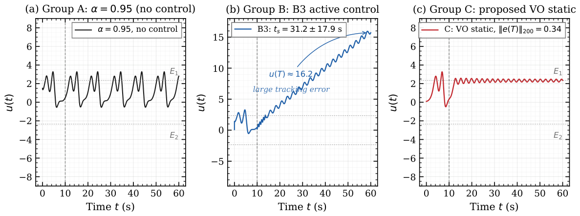
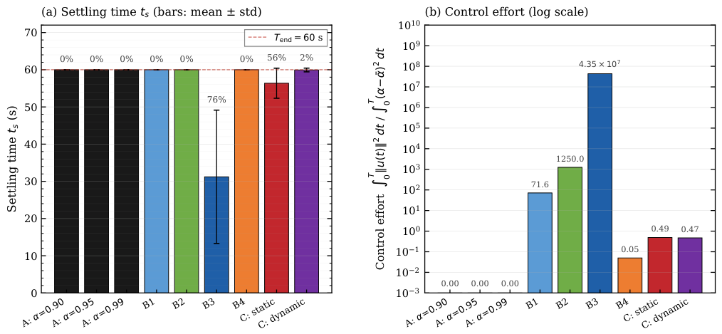
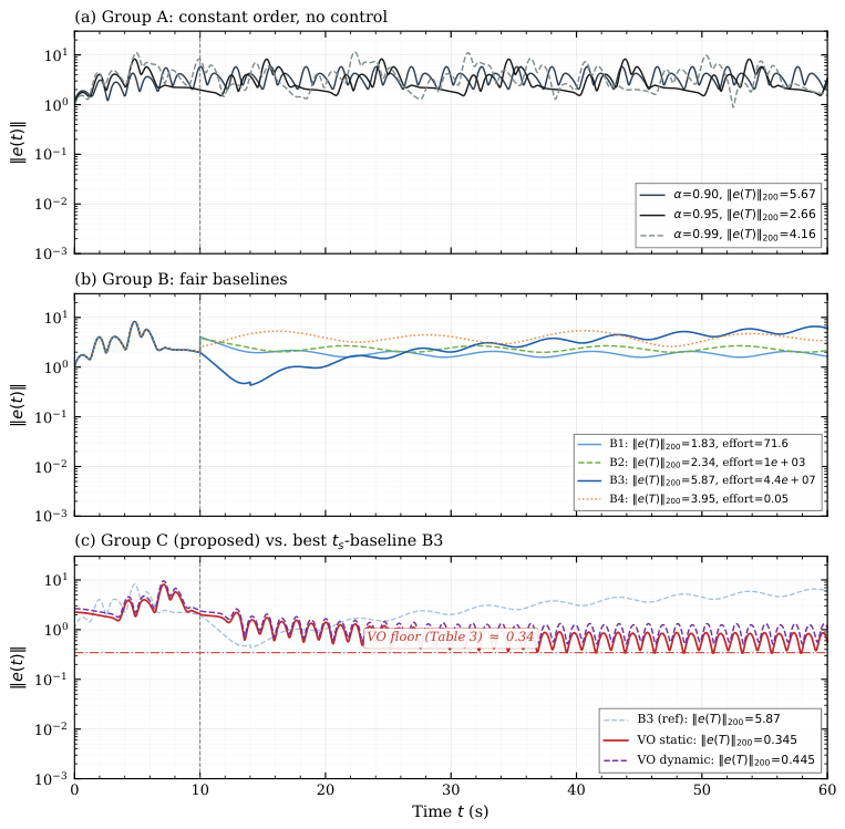
For the VO controllers, the effective effort is $E_{\mathrm{vo}}={\int }_0^T{|\alpha \left(t\right)-\overline{\alpha }|}^2 dt$. For B1–B3, the standard $E={\int }_0^T{\parallel \mathbf{u}\left(t\right)\parallel }^2 dt$ is used. Baseline B1 is tuned so that its effort matches $E_{\mathrm{vo}}$, ensuring a fair energy-equivalent comparison. Representative state-variable trajectories under the three control regimes (Group A, Group B baseline B3, and Group C proposed VO law) are shown in Figure 6. The corresponding settling-time and control-effort summary across all baselines is given in Figure 7, and the time evolution of the tracking-error norm $\parallel e\left(t\right)\parallel$ on a logarithmic scale is shown in Figure 8.

6. Conclusions and Future Works

This paper presented a state-dependent order modulation strategy for chaos control and hybrid synchronization in the variable-order fractional Arneodo system, where the differentiation order $\alpha \left(t\right)$ is used directly as the control input via the Liouville–Caputo operator. Static and dynamic modulation laws driven by a hybrid chaos indicator were implemented and compared with classical controllers. The present prescriptive (control-oriented) framework complements the recent descriptive (dynamics-oriented) studies of variable-order Arneodo and Newton–Leipnik systems [27,28], providing the closed-loop counterpart to those open-loop analyses.

Local existence and uniqueness were established through the Volterra integral formulation and the Banach fixed-point theorem. Local stability of the nontrivial equilibria $E_{1,2}$ was analyzed via Matignon’s spectral criterion under the quasi-static approximation, identifying the closed-form critical order ${\alpha }_c=(2/\pi )arctan\left(\sqrt{21}\right)\approx 0.8632$, which the closed-loop modulation law actively traverses to suppress chaos. A second-order predictor–corrector scheme was used and observed to attain its expected $O\left(h^2\right)$ convergence rate.

Comprehensive numerical experiments (200 independent Monte Carlo runs) revealed a distinctive performance profile. The proposed VO static law achieves a terminal tracking error of $0.345$ (in the 2-norm to the nearest equilibrium $E_{1,2}$), an 81% reduction relative to the best fixed-order indicator-feedback baseline (${\parallel e\left(T\right)\parallel }_{\mathrm{B}1}=1.83$). The VO laws also exhibit an effort budget of ∼0.5 (in the integrated order-excursion sense), which is approximately eight orders of magnitude smaller than the classical active controller (B3, effort $\approx 4.35\times {10}^7$ in the integrated control input squared sense), while attaining a 17 times smaller terminal tracking error than B3. The trade-off is therefore explicit: B3 captures slightly faster, but at substantially higher effort and worse terminal accuracy. In contexts where precision and energy efficiency matter more than transient speed, the proposed VO laws are Pareto-optimal among the tested methods.

The strategy also achieved hybrid synchronization (complete in $(u,v)$ and anti-synchronization in w) in the variable-order setting. Future work could include experimental validation on chaotic electronic circuits and extension to multi-agent networked systems [11,61].

Future Work

Several directions naturally extend the present framework:

(1)

Stability beyond the local, quasi-static picture, via radially unbounded or non-quadratic (polynomial / sum-of-squares) Lyapunov constructions that yield basin-of-attraction estimates and remain valid near the bifurcation $\alpha \left(t\right)={\alpha }_c$;

(2)

A non-autonomous extension of Matignon’s theory, providing quantitative bounds on the admissible variation rate $|\dot{\alpha }\left(t\right)|$ together with sharper predictor–corrector error constants for Type I and a comparison with Types II and III;

(3)

Learning-based order modulation, in which $\alpha \left(t\right)$ is optimized online under actuator constraints by reinforcement learning;

(4)

Networked and cross-operator extensions, coupling variable-order Arneodo oscillators for secure communication and validating the framework under Type II Liouville–Caputo formulations with matched modulation laws;

(5)

Hardware realization of the Oustaloup-based switched-bank and lookup-table strategies of Section 4.3.2, with FPGA (Xilinx Artix-7 class) and ARM Cortex-M4 hardware-in-the-loop validation.

References

1. Podlubny, I. Index. In Fractional Differential Equations: An Introduction to Fractional Derivatives, Fractional Differential Equations, to Methods of Their Solution and Some of Their Applications; Academic Press: Cambridge, MA, USA, 1999; pp. 337–340. [Google Scholar] [CrossRef]
2. Kilbas, A.A.; Srivastava, H.M.; Trujillo, J.J. Theory and Applications of Fractional Differential Equations; North-Holland Mathematics Studies; Elsevier: Amsterdam, The Netherlands, 2006; Volume 204. [Google Scholar] [CrossRef]
3. Diethelm, K. Multi-Term Caputo Fractional Differential Equations. In The Analysis of Fractional Differential Equations; Springer: Berlin/Heidelberg, Germany, 2010; pp. 167–186. [Google Scholar] [CrossRef]
4. Kahouli, O.; Djenina, N.; Ouannas, A.; Alshammari, B.M.; Aloui, A.; Abidi, I. Chaos control in discrete fractional systems with variable order: Analysis and numerical simulations. Electron. Res. Arch. 2026, 34, 55–68. [Google Scholar] [CrossRef]
5. Samko, S.G.; Ross, B. Integration and differentiation to a variable fractional order. Integral Transform. Spec. Funct. 1993, 1, 277–300. [Google Scholar] [CrossRef]
6. Coimbra, C.F.M. Mechanics with variable-order differential operators. Ann. Phys. 2003, 515, 692–703. [Google Scholar] [CrossRef]
7. Abdulrhman, T. Stability Analysis of Fractional Chaotic and Fractional-Order Hyperchain Systems Using Lyapunov Functions. Eur. J. Pure Appl. Math. 2025, 18, 5576. [Google Scholar] [CrossRef]
8. Lorenzo, C.F.; Hartley, T.T. Variable order and distributed order fractional operators. Nonlinear Dyn. 2002, 29, 57–98. [Google Scholar] [CrossRef]
9. Sun, H.; Chen, W.; Chen, Y. Variable-order fractional differential operators in anomalous diffusion modeling. Phys. Stat. Mech. Its Appl. 2009, 388, 4586–4592. [Google Scholar] [CrossRef]
10. Almatroud, O.A.; Hioual, A.; Ouannas, A.; Sawalha, M.M.; Alshammari, S.; Alshammari, M. On Variable-Order Fractional Discrete Neural Networks: Existence, Uniqueness and Stability. Fractal Fract. 2023, 7, 118. [Google Scholar] [CrossRef]
11. Awad, Y.; Fakih, H.; Alkhezi, Y. Existence and Uniqueness of Variable-Order ϕ-Caputo Fractional Two-Point Nonlinear Boundary Value Problem in Banach Algebra. Axioms 2023, 12, 935. [Google Scholar] [CrossRef]
12. Tavares, D.; Almeida, R.; Torres, D.F.M. Caputo derivatives of fractional variable order: Numerical approximations. Commun. Nonlinear Sci. Numer. Simul. 2016, 35, 2. [Google Scholar] [CrossRef]
13. Moghaddam, B.P.; Yaghoobi, S.; Machado, J.A.T. An Extended Predictor–Corrector Algorithm for Variable-Order Fractional Delay Differential Equations. J. Comput. Nonlinear Dyn. 2016, 11, 061001. [Google Scholar] [CrossRef]
14. Wang, C.; Zhou, X.; Shi, X.; Jin, Y. Delay-dependent and order-dependent stability and stabilization analysis of variable fractional order uncertain differential systems with time-varying delay via linear matrix inequality approach. J. Vib. Control. 2022, 29, 2763–2773. [Google Scholar] [CrossRef]
15. Arneodo, A.; Coullet, P.; Peyraud, J.; Tresser, C. Strange Attractors in Volterra Equations for Species in Competition. J. Math. Biol. 1982, 14, 153–157. [Google Scholar] [CrossRef] [PubMed]
16. Arneodo, A.; Coullet, P.; Tresser, C. Possible New Strange Attractors with Spiral Structure. Commun. Math. Phys. 1981, 79, 573–579. [Google Scholar] [CrossRef]
17. Tavazoei, M.S.; Haeri, M. A necessary condition for double scroll attractor existence in fractional-order systems. Phys. Lett. A 2007, 367, 102–113. [Google Scholar] [CrossRef]
18. Tavazoei, M.S.; Haeri, M. Synchronization of chaotic fractional-order systems via active sliding mode controller. Phys. A Stat. Mech. Its Appl. 2008, 387, 57–70. [Google Scholar] [CrossRef]
19. Lu, J.G. Chaotic dynamics and synchronization of fractional-order Arneodo’s systems. Chaos Solitons Fractals 2005, 26, 1125–1133. [Google Scholar] [CrossRef]
20. Gokyildirim, A.; Akgul, A.; Calgan, H.; Demirtas, M. Parametric fractional-order analysis of Arneodo chaotic system and microcontroller-based secure communication implementation. AEU-Int. J. Electron. Commun. 2024, 175, 155080. [Google Scholar] [CrossRef]
21. Elbadri, M.; Ashmaig, M.A.M.; Hassan, A.A.; Hdidi, W.; Barakat, H.M.; Al-Mutairi, G.S.; Abdoon, M.A. Exploring Stability and Chaos in the Fractional-Order Arneodo System via Grünwald–Letnikov Scheme. Mathematics 2025, 13, 3925. [Google Scholar] [CrossRef]
22. Matouk, A.E. Chaos, feedback control and synchronization of a fractional-order modified Autonomous Van der Pol–Duffing circuit. Commun. Nonlinear Sci. Numer. Simul. 2011, 16, 975–986. [Google Scholar] [CrossRef]
23. Jiang, J.; Xu, X.; Zhao, K.; Guirao, J.L.G.; Saeed, T.; Chen, H. The Tracking Control of the Variable-Order Fractional Differential Systems by Time-Varying Sliding-Mode Control Approach. Fractal Fract. 2022, 6, 231. [Google Scholar] [CrossRef]
24. Li, C.; Chen, G. Chaos in the fractional order Chen system and its control. Chaos Solitons Fractals 2004, 22, 549–554. [Google Scholar] [CrossRef]
25. Ojo, K.S.; Ogunjo, S.T.; Fuwape, I.A. Modified hybrid combination synchronization of chaotic fractional order systems. Soft Comput. 2022, 26, 11865–11872. [Google Scholar] [CrossRef]
26. Khalid, T.A. Generalized Controllability, Stability, and Chaos in Fractional Dynamics: A Unified Approach. Int. J. Basic Appl. Sci. 2026, 14, 652–659. [Google Scholar] [CrossRef]
27. Elbadri, M.; Al-kuleab, N.; Saadeh, R.; Abdalla, A.H.; Jazmati, M.S.; Abdoon, M.A.; Hafez, M. Study of the Variable-Order Fractional Arneodo System: Bifurcation, Chaos, and Dynamic Behavior. Fractal Fract. 2026, 10, 296. [Google Scholar] [CrossRef]
28. Saadeh, R.; Taha, N.E.; Hafez, M.; Al-Mutairi, G.S.; Ashmaig, M.A.M. Dynamics and Solution Behavior of the Variable-Order Fractional Newton–Leipnik System. Mathematics 2026, 14, 312. [Google Scholar] [CrossRef]
29. Patnaik, S.; Hollkamp, J.P.; Semperlotti, F. Applications of variable-order fractional operators: A review. Proc. R. Soc. Math. Phys. Eng. Sci. 2020, 476, 20190498. [Google Scholar] [CrossRef]
30. Hosbas, M.Z.; Emin, B.; Kacar, F. True Random Number Generator Design with A Fractional Order Sprott B Chaotic System. ADBA Comput. Sci. 2025, 2, 50–55. [Google Scholar] [CrossRef]
31. Kopp, M.; Samuilik, I. A New 6D Two–wing Hyperchaotic System: Dynamical Analysis, Circuit Design, and Synchronization. Chaos Theory Appl. 2024, 6, 273–283. [Google Scholar] [CrossRef]
32. Abbas, A.; Khaliq, A. Nonlinear Dynamics and Chaos Control in a Discrete Sel’kov Model with Substrate Inhibition. Chaos Fractals 2026, 3, 29–37. [Google Scholar] [CrossRef]
33. Almeida, R.; Tavares, D.; Torres, D.F.M. The Variable-Order Fractional Calculus of Variations. In The Fractional Calculus of Variations; Springer: Cham, Switzerland, 2018; pp. 61–113. [Google Scholar] [CrossRef]
34. Xu, Y.; He, Z. Existence and uniqueness results for Cauchy problem of variable-order fractional differential equations. J. Appl. Math. Comput. 2013, 43, 295–306. [Google Scholar] [CrossRef]
35. Moualkia, S.; Xu, Y. On the Existence and Uniqueness of Solutions for Multidimensional Fractional Stochastic Differential Equations with Variable Order. Mathematics 2021, 9, 2106. [Google Scholar] [CrossRef]
36. Wu, G.-C.; Deng, Z.-G.; Baleanu, D.; Zeng, D.-Q. New variable-order fractional chaotic systems for fast image encryption. Chaos Interdiscip. J. Nonlinear Sci. 2019, 29, 083103. [Google Scholar] [CrossRef]
37. Zhang, S. The uniqueness result of solutions to initial value problems of differential equations of variable-order. Rev. Real Acad. Cienc. Exactas Físicas Nat. Ser. A Mat. 2017, 112, 407–423. [Google Scholar] [CrossRef]
38. Benkerrouche, A.; Souid, M.S.; Karapınar, E.; Hakem, A. On the boundary value problems of Hadamard fractional differential equations of variable order. Math. Methods Appl. Sci. 2022, 46, 3187–3203. [Google Scholar] [CrossRef]
39. Wang, F.; Liu, L. The Existence and Uniqueness of Solutions for Variable-Order Fractional Differential Equations with Antiperiodic Fractional Boundary Conditions. J. Funct. Spaces 2022, 2022, 7663192. [Google Scholar] [CrossRef]
40. O’Regan, D.; Agarwal, R.P.; Hristova, S.; Abbas, M.I. Existence and Stability Results for Differential Equations with a Variable-Order Generalized Proportional Caputo Fractional Derivative. Mathematics 2024, 12, 233. [Google Scholar] [CrossRef]
41. Ye, H.; Gao, J.; Ding, Y. A generalized Gronwall inequality and its application to a fractional differential equation. J. Math. Anal. Appl. 2007, 328, 1075–1081. [Google Scholar] [CrossRef]
42. Gradshteyn, I.S.; Ryzhik, I.M. Indefinite integrals of special functions. In Table of Integrals, Series, and Products; Academic Press: Cambridge, MA, USA, 1980; pp. 626–634. [Google Scholar] [CrossRef]
43. Telli, B.; Souid, M.S.; Alzabut, J.; Khan, H. Existence and Uniqueness Theorems for a Variable-Order Fractional Differential Equation with Delay. Axioms 2023, 12, 339. [Google Scholar] [CrossRef]
44. Petráš, I. Fractional-Order Systems. In Fractional-Order Nonlinear Systems; Springer: Berlin/Heidelberg, Germany, 2011; pp. 43–54. [Google Scholar] [CrossRef]
45. Li, Y.; Chen, Y.; Podlubny, I. Mittag–Leffler stability of fractional order nonlinear dynamic systems. Automatica 2009, 45, 1965–1969. [Google Scholar] [CrossRef]
46. Matignon, D. Stability results for fractional differential equations with applications to control processing. In Proceedings of the Computational Engineering in Systems Applications, Lille, France, 9–12 July 1996; IMACS: Lille, France, 1996; Volume 2, pp. 963–968. [Google Scholar]
47. Aguila-Camacho, N.; Duarte-Mermoud, M.A.; Gallegos, J.A. Lyapunov functions for fractional order systems. Commun. Nonlinear Sci. Numer. Simul. 2014, 19, 2951–2957. [Google Scholar] [CrossRef]
48. Rosenstein, M.T.; Collins, J.J.; Luca, C.J.D. A practical method for calculating largest Lyapunov exponents from small data sets. Phys. Nonlinear Phenom. 1993, 65, 117–134. [Google Scholar] [CrossRef]
49. Abed-Elhameed, T.M.; Aboelenen, T. Mittag–Leffler stability, control, and synchronization for chaotic generalized fractional-order systems. Adv. Contin. Discret. Model. 2022, 2022, 50. [Google Scholar] [CrossRef]
50. Vaidyanathan, S.; Rasappan, S. Hybrid Synchronization of Arneodo and Rössler Chaotic Systems by Active Nonlinear Control. In Advances in Computer Science and Information Technology. Networks and Communications; Springer: Berlin/Heidelberg, Germany, 2012; pp. 73–82. [Google Scholar] [CrossRef]
51. Khan, A.; Khattar, D.; Agrawal, N. Synchronization of a new fractional order chaotic system. Int. J. Dyn. Control. 2017, 6, 1585–1591. [Google Scholar] [CrossRef]
52. Oustaloup, A.; Levron, F.; Mathieu, B.; Nanot, F.M. Frequency-band complex noninteger differentiator: Characterization and synthesis. IEEE Trans. Circuits Syst. Fundam. Theory Appl. 2000, 47, 25–39. [Google Scholar] [CrossRef]
53. Chua, L.; Komuro, M.; Matsumoto, T. The double scroll family. IEEE Trans. Circuits Syst. 1986, 33, 1072–1118. [Google Scholar] [CrossRef]
54. Tepljakov, A. Introduction. In Fractional-Order Modeling and Control of Dynamic Systems; Springer: Cham, Switzerland, 2017; pp. 1–10. [Google Scholar] [CrossRef]
55. Sierociuk, D.; Malesza, W.; Macias, M. Derivation, interpretation, and analog modelling of fractional variable order derivative definition. Appl. Math. Model. 2015, 39, 3876–3888. [Google Scholar] [CrossRef]
56. Diethelm, K.; Ford, N.J. Multi-order fractional differential equations and their numerical solution. Appl. Math. Comput. 2004, 154, 621–640. [Google Scholar] [CrossRef]
57. Garrappa, R. Numerical Solution of Fractional Differential Equations: A Survey and a Software Tutorial. Mathematics 2018, 6, 16. [Google Scholar] [CrossRef]
58. Garrappa, R.; Giusti, A. A Computational Approach to Exponential-Type Variable-Order Fractional Differential Equations. J. Sci. Comput. 2023, 96, 63. [Google Scholar] [CrossRef]
59. Taha, N.E. Chaotic Dynamics and Numerical Solutions of the Stochastic Fractional-Order Lorenz System. J. Qassim Univ. Sci. 2026, 5, 2. [Google Scholar] [CrossRef]
60. Romano, J.; Kromrey, J.D.; Coraggio, J.; Skowronek, J.; Devine, L. Exploring methods for evaluating group differences on the NSSE and other surveys: Are the t-test and Cohen’s d indices the most appropriate choices. In Proceedings of the Annual Meeting of the Southern Association for Institutional Research, Arlington, VA, USA, 15–17 October 2006; Citeseer: University Park, PA, USA, 2006; Volume 14. [Google Scholar]
61. Li, H.-L.; Hu, C.; Jiang, Y.-L.; Zhang, L.; Teng, Z. Global Mittag–Leffler stability for a coupled system of fractional-order differential equations on network with feedback controls. Neurocomputing 2016, 214, 233–241. [Google Scholar] [CrossRef]
Figure 1. Examples of admissible variable-order functions α ( t ) used in this work. Horizontal axis: time t in seconds; vertical axis: dimensionless fractional order α ( t ) [ 0.85 ,   0.99 ] . The four profiles shown are: sinusoidal α ( t ) = 0.95 + 0.04 sin ( t ) ; sigmoidal α ( t ) = 0.9 + 0.09 tanh ( t / 10 ) ; piecewise constant; and the linear-with-saturation profile α ( t ) = min ( 0.85 + 0.003   t ,   0.99 ) , which saturates at t = 46.7 s.
Fractalfract 10 00376 g001
Figure 2. Numerical verification of the critical fractional order α c 0.8632 predicted by Matignon’s criterion for the constant-order Arneodo system at E 1 , 2 . (Top row): Phase portraits in the ( u , w ) plane. (Bottom row): Time series u ( t ) , with horizontal dotted lines at u = ± 5.5 marking the projections of E 1 , 2 . (Left) ( α = 0.84 < α c ): The trajectory converges to E 1 , in agreement with Theorem 4. (Centre) ( α = 0.86 α c ): A long oscillatory transient near E 1 reflects the proximity to the bifurcation. (Right) ( α = 0.88 > α c ): Sustained oscillatory dynamics indicate loss of local stability of E 1 , 2 . Initial condition ( u 0 , v 0 , w 0 ) = ( 0.5 , 0.5 , 0.5 ) , step size h = 0.01 , time horizon T = 60 .
Fractalfract 10 00376 g002
Figure 3. 3D attractors for constant, sinusoidal, sigmoidal, and piecewise α ( t ) .
Fractalfract 10 00376 g003
Figure 4. Bifurcation diagram of the constant-order fractional Arneodo system as a function of the fractional order α [ 0.88 ,   1.00 ] . Horizontal axis: fractional order α (dimensionless); vertical axis: dimensionless local maxima and minima of u ( t ) recorded over the post-transient interval t [ 200 ,   500 ] s with step size h = 0.01 . The transition from a periodic to chaotic regime occurs near α 0.94 .
Fractalfract 10 00376 g004
Figure 5. Bifurcation diagram of the variable-order Arneodo system under the sinusoidal profile α ( t ) = 0.95 + A sin ( t ) , as a function of the modulation amplitude A. Horizontal axis: amplitude A [ 0 ,   0.10 ] (dimensionless); vertical axis: dimensionless local maxima and minima of u ( t ) over the post-transient interval t [ 200 ,   500 ] s with step size h = 0.01 . The chaotic regime is preserved across the entire amplitude range.
Fractalfract 10 00376 g005
Figure 6. Representative state-variable trajectories u ( t ) obtained from the Grünwald–Letnikov solver of Section 5.1 (single Monte Carlo run; identical seed across panels). Vertical dashed line marks control activation at t = 10 s; dotted horizontal lines mark the projections of the equilibria E 1 , 2 = ( ± 5.5 ,   0 ,   0 ) on the u-axis. (a) Group A (constant α = 0.95 , no control): the trajectory exhibits sustained chaotic oscillation, consistent with α > α c and the resulting instability of E 1 , 2 predicted by Theorem 4. (b) Group B (B3, active controller applied at constant α = 0.95 ; controller form follows the active-control methodology described in Section 4.2): the trajectory diverges to u ( T ) 16 , illustrating the large terminal tracking error ( e ( T ) 200 5.87 in Table 4) despite the favourable settling time of B3. (c) Group C (proposed VO static law): the closed-loop trajectory is captured into a tight neighbourhood of E 1 2.345 , consistent with the terminal tracking error e ( T ) 200 = 0.345 reported in Table 4. Each panel shows its own vertical axis (labeled u ( t ) , with independent tick range), so the reader can read off the trajectory amplitude directly in every regime. Statistical metrics in the legends are mean values across the N MC = 200 runs of Table 4.
Fractalfract 10 00376 g006
Figure 7. Summary of the controlled ablation study (Table 4, N MC = 200 runs per method). (a) Settling time t s (mean ± standard deviation). The horizontal dashed red line marks the simulation horizon T end = 60 s; bars reaching this line indicate that the corresponding method failed to capture the trajectory into a δ s = 0.5 neighbourhood of E 1 , 2 within the simulation horizon. Numbers above each bar denote the empirical settled fraction (fraction of Monte Carlo runs that reached the capture criterion). B3 (active control) attains the fastest settling time but with substantial run-to-run variability, while the proposed VO static law settles in 56.4 ± 4.0 s in 56 % of runs. (b) Total control effort on logarithmic scale. For B1–B3 the effort is the integrated control input squared E = 0 T u ( t ) 2   d t ; for the VO methods (B4 and Group C) the effort is the integrated order excursion E vo = 0 T ( α ( t ) α ¯ ) 2   d t , which directly quantifies the control activity in the order modulation framework. Note the eight orders of magnitude gap between the proposed VO laws ( 0.5 ) and the active controller B3 (≈4.4 × 10 7 ).
Fractalfract 10 00376 g007
Figure 8. Time evolution of the tracking-error norm e ( t ) = min { x ( t ) E 1 ,   x ( t ) E 2 } on a logarithmic scale, for the same representative trajectories as in Figure 6. The vertical dashed line marks control activation at t = 10 s. (a) Group A (constant order, no control): all three fixed- α regimes exhibit sustained oscillation around the chaotic-attractor scale, with e ( t ) remaining at order 1–10 throughout the post-control phase. (b) Group B (fair baselines): B1 (energy-equivalent indicator-feedback) and B2 (sliding mode) reduce the error to a plateau near e ( t ) 2 but do not capture the trajectory; B3 (active control) initially decreases e ( t ) but subsequently drifts to large values; B4 (predetermined VO with no feedback) preserves the chaotic regime. (c) Group C (proposed) versus the best t s -baseline B3: both VO laws drive e ( t ) down toward the empirical floor 0.34 (red dash–dot line, taken from Table 4), substantially below all baselines. The legend reports the mean terminal error e ( T ) 200 from the N MC = 200 Monte Carlo runs.
Fractalfract 10 00376 g008