Hybrid Modeling of Long-Memory Degradation Dynamics Using Fractional Difference Operators and Deep Reinforcement Learning

Abstract

Long-memory degradation processes in rotating machinery often exhibit nonlinear evolution, nonlocal temporal dependence, and hereditary characteristics, which are difficult to fully capture using conventional integer-order models or standard Markovian decision frameworks. To address this issue, this study proposes a hybrid fractional-dynamics and deep reinforcement learning framework for predictive maintenance of memory-dependent degradation systems. First, the Grünwald–Letnikov fractional difference operator is introduced to construct a fractional-memory representation of degradation trajectories, enabling the model to explicitly encode long-range dependence and accumulated historical degradation effects. Then, a bidirectional gated recurrent unit network is employed to learn sequential degradation representations from the fractional-memory state space, while a deep Q-network is designed to optimize maintenance decisions under uncertain degradation evolution. Experimental results on the IEEE PHM 2012 bearing dataset show that the proposed FM-BiGRU-DQN with safety-guided execution achieved a mean maintenance lead time of 33.9 ± 12.6 steps, an in-band rate of 0.85 ± 0.06, a failure rate of 0.00 ± 0.00, and a deployment reliability of 1.00 ± 0.00 over 10 independent random seeds. Compared with NM-BiGRU-DQN, the in-band rate increased from 0.55 ± 0.10 to 0.85 ± 0.06, with a paired-test p-value of 0.013. Cross-dataset validation on the XJTU-SY bearing dataset further achieved an in-band rate of 0.80 and a failure rate of 0.00. These results indicate that embedding fractional-memory dynamics into deep reinforcement learning improves maintenance timing accuracy, policy robustness, and deployment reliability for complex memory-dependent degradation systems.

1. Introduction

Predictive maintenance (PdM) has become an essential strategy for improving the reliability, availability, and cost efficiency of complex industrial systems. With the rapid development of the Industrial Internet of Things (IIoT), large volumes of condition-monitoring data can now be continuously collected from rotating machinery, providing a data basis for health assessment, remaining useful life (RUL) prediction, and maintenance decision-making. In recent years, deep-learning-enabled PdM has received increasing attention because of its capability to extract nonlinear degradation patterns from high-dimensional monitoring signals. Wang et al. [1] systematically reviewed deep-learning-based PdM methods in IIoT environments and summarized their major methodologies, applications, and challenges. In addition, reinforcement learning has been increasingly introduced into PdM because maintenance optimization is naturally a sequential decision-making problem under uncertainty. Aglogallos et al. [2] investigated health-state prediction with reinforcement learning for predictive maintenance, indicating the potential of learning-based approaches in adaptive maintenance decision support.

Although data-driven deep learning and reinforcement learning methods have achieved promising results, many existing PdM studies still rely implicitly on short-memory or Markovian assumptions. In such formulations, either the current observation or a short temporal window is assumed to contain sufficient information for prediction or decision-making. However, degradation processes in rotating machinery are usually cumulative, nonlinear, and history-dependent. The current health state of a bearing may be affected not only by recent vibration changes but also by long-term damage accumulation, crack propagation, and persistent degradation trends. Therefore, the degradation trajectory often exhibits long-memory, nonlocal temporal dependence, and hereditary characteristics. These properties are difficult to fully represent using conventional integer-order models, standard Markov decision processes, or purely data-driven feature representations.

Fractional-order modeling provides a natural mathematical tool for describing memory-dependent and hereditary phenomena. Different from integer-order operators, fractional operators incorporate historical information through nonlocal kernels and can represent the influence of past states on current system evolution. This characteristic makes fractional calculus suitable for complex dynamical systems in which long-range dependence plays an important role. Recent studies have begun to introduce fractional-order ideas into prognostics, reliability modeling, and industrial monitoring. Awadalla and Murugesan [3] proposed Bayesian fractional Weibull regression for reliability prognostics and predictive maintenance, showing that fractional modeling can support maintenance-related reliability analysis. Gomolka et al. [4] developed a fractional-order neural network for detecting process deviations in optical fiber cable manufacturing, demonstrating the applicability of fractional-order learning models in industrial systems. These studies suggest that fractional-order methods can provide useful memory-aware representations for degradation modeling and industrial decision-making.

In parallel, reinforcement-learning-based maintenance optimization has attracted increasing research interest. Since maintenance actions must be selected dynamically according to evolving degradation states, deep reinforcement learning offers a flexible framework for optimizing long-term maintenance rewards under uncertainty. Supramaniam et al. [5] studied predictive maintenance using deep reinforcement learning. Ding et al. [6] integrated RUL prediction with multi-agent deep reinforcement learning for adaptive real-time production and maintenance scheduling. Faizanbasha and Rizwan [7] proposed a deep learning–stochastic ensemble for RUL prediction and predictive maintenance with dynamic mission abort policies. These studies demonstrate that reinforcement learning can support adaptive maintenance policy learning. Nevertheless, most reinforcement-learning-based PdM methods still formulate the degradation environment as a Markov decision process and do not explicitly encode long-memory degradation dynamics into the state representation.

Deep neural architectures have also been widely used to improve degradation representation and prognostic performance. Xiao et al. [8] proposed a convolutional neural network–bidirectional gated recurrent unit (CNN-BiGRU) predictive maintenance method enhanced by an attention mechanism application in industrial equipment. Solichin et al. [9] integrated optimum feature extraction with a transformer network for rolling bearing RUL prediction. In addition, Yu and Caspary [10] investigated Teager–Kaiser energy operator (TKEO)-enhanced machine learning for bearing fault classification in predictive maintenance. Nastasi [11] summarized emerging artificial intelligence (AI)-based predictive maintenance techniques for bearings and discussed related engineering solutions. Yang et al. [12] proposed an uncertainty-aware predictive maintenance framework using a hybrid Transformer with Monte Carlo Dropout and conformal prediction. Sun et al. [13] proposed a bearing RUL prognostics method based on convolution attention networks and an enhanced transformer. Jagdale et al. [14] reviewed digital-twin-driven predictive maintenance for induction motor bearing fault detection and prognostics. These studies show that modern PdM is moving toward increasingly intelligent and data-intensive frameworks. However, deep learning models usually learn temporal patterns from data in an implicit manner. Without an explicit memory-aware mechanism, the learned representation may still be insufficient for describing nonlocal degradation evolution, especially when the degradation trajectory exhibits clear long-range dependence.

Therefore, an important research gap remains: integrating fractional-order memory modeling with deep reinforcement learning for predictive maintenance of long-memory degradation systems. For one, fractional operators can provide an explicit representation of historical degradation effects and nonlocal temporal dependence. Furthermore, deep neural networks and reinforcement learning can learn nonlinear degradation representations and optimize maintenance actions under uncertainty. A hybrid modeling framework that combines these two advantages is expected to reduce the mismatch between non-Markovian degradation behavior and Markovian decision-making assumptions. Such a framework is also consistent with the broader development of hybrid modeling approaches that combine fractional dynamics, deep learning, and data-driven decision optimization for complex systems.

Motivated by this gap, this study proposes a hybrid fractional-dynamics and deep reinforcement learning framework for the predictive maintenance of long-memory degradation systems. Specifically, the Grünwald–Letnikov fractional difference operator is introduced to construct a fractional-memory representation of degradation trajectories. This representation is designed to encode long-range dependence and accumulated historical degradation effects before policy learning. A bidirectional gated recurrent unit (BiGRU) network is then employed to extract sequential degradation representations from the fractional-memory state space, and a deep Q-network (DQN) is used to learn adaptive maintenance policies. In this way, the proposed framework integrates fractional-memory degradation modeling, deep sequence representation learning, and reinforcement-learning-based maintenance optimization into a unified decision-making architecture.

The main contributions of this study are summarized as follows:

• A fractional-memory state representation is constructed for long-memory degradation trajectories using the Grünwald–Letnikov fractional difference operator, enabling nonlocal and hereditary degradation information to be explicitly embedded into the decision state.
• A hybrid fractional-dynamics and deep reinforcement learning framework, termed fractional-memory BiGRU-DQN (FM-BiGRU-DQN), is developed by integrating fractional-memory state construction, bidirectional gated recurrent unit (BiGRU)-based sequential representation learning, and deep Q-network (DQN)-based maintenance policy optimization.
• The predictive maintenance problem is reformulated as a fractional-state sequential decision problem, which helps reduce the mismatch between long-memory degradation evolution and conventional Markovian decision assumptions.
• Comparative experiments, fractional-order sensitivity analysis, and safety-guided policy evaluation are conducted on rolling bearing degradation data to verify the effectiveness, robustness, and deployment reliability of the proposed framework.

The remainder of this paper is organized as follows. Section 2 introduces the theoretical background and formulates predictive maintenance as a fractional-state sequential decision problem. Section 3 presents the proposed FM-BiGRU-DQN framework, including health indicator construction, fractional-state generation, Q-network learning, and safety-guided policy execution. Section 4 reports the experimental results and discusses the effectiveness of the proposed method. Section 5 concludes the paper and outlines future research directions.

2. Theoretical Background and Problem Formulation

2.1. Long-Memory Degradation Dynamics in Predictive Maintenance

In predictive maintenance, degradation evolution is often simplified as a Markovian process, in which the future state and maintenance decision are assumed to depend only on the current observation [15]. This assumption is convenient for reinforcement learning, but it may be insufficient for rolling bearing degradation. In practical rotating machinery, bearing degradation is a cumulative damage process involving crack initiation, propagation, surface fatigue, and local defect expansion. Therefore, the current health condition is affected not only by the latest observation, but also by historical degradation accumulation over a relatively long horizon [16].

Let the health indicator sequence extracted from the bearing vibration signal be denoted as

$$x=\{x_1,x_2,\dots ,x_N\}$$

(1)

where $x_t$ represents the health indicator at time step $t$, and $N$ is the length of the degradation trajectory. If the degradation process has long-memory characteristics, the future degradation state cannot be fully determined by the current observation alone. In other words,

$$P(x_{t+1}|x_t,a_t)\ne P(x_{t+1}|x_t,x_{t-1},\dots ,x_1,a_t)$$

(2)

where $a_t$ denotes the maintenance action at time step $t$. This indicates that the standard Markovian state representation may lose useful historical degradation information.

To verify the long-memory property of the degradation trajectory, the Hurst exponent is estimated using rescaled range analysis. For a subsequence of length $n$, the local mean is defined as

$${\overline{x}}_n={\displaystyle \frac{1}{n}}{\displaystyle \sum _{t=1}^n{x}_t}$$

(3)

The cumulative deviation sequence is calculated as

$$Y(k,n)={\displaystyle \sum _{t=1}^k(x_t-{\overline{x}}_n)},k=1,2,\dots ,n$$

(4)

The range $R\left(n\right)$ and standard deviation $S\left(n\right)$ are then defined as

$$R(n)={\max }_{1\le k\le n}Y(k,n)-{\min }_{1\le k\le n}Y(k,n)$$

(5)

$$S(n)=\sqrt{{\displaystyle \frac{1}{n}}{\displaystyle \sum _{t=1}^n{(x_t-{\overline{x}}_n)}^2}}$$

(6)

The rescaled range statistic satisfies the following scaling relation:

$${\displaystyle \frac{R(n)}{S(n)}}=C{n}^H$$

(7)

where $C$ is a constant and $H$ is the Hurst exponent. Taking logarithms on both sides gives

$$\log \left({\displaystyle \frac{R(n)}{S(n)}}\right)=\log C+H\log n.$$

(8)

Therefore, $H$ can be estimated as the slope of the linear fitting curve in the log-log coordinate system.

The value of $H$ reflects the memory property of the degradation sequence. When $H=0.5$, the sequence behaves similarly to a memoryless random walk. When $H>0.5$, the sequence exhibits persistence, indicating that past degradation trends are likely to continue. When $H<0.5$, the sequence is anti-persistent. In the context of bearing degradation, an empirical value of $H>0.5$ suggests that the degradation process contains long-range dependence and should not be treated as a purely Markovian process. This provides the motivation for introducing a fractional-memory representation into the maintenance decision model.

It should be emphasized that the standard Hurst exponent is theoretically bounded within $0<H<1$. Therefore, an R/S-fitted slope larger than 1 cannot be interpreted as a valid Hurst exponent. In run-to-failure bearing degradation trajectories, strong monotonic trends, finite sample length, and nonstationary behavior near failure may bias the classical R/S estimate upward. For this reason, the R/S result in this study is used only as a preliminary scaling diagnostic rather than as a definitive Hurst-exponent estimate. To obtain a more robust assessment of persistence, we further apply detrended fluctuation analysis (DFA), which reduces the influence of local trends before estimating the fluctuation-scaling exponent.

2.2. Fractional Calculus for Degradation Memory Representation

Once the long-memory property of bearing degradation has been identified, the next problem is how to represent this memory in a compact and mathematically meaningful form. A simple approach is to stack historical observations into the state. However, this strategy may introduce redundant information and does not explicitly characterize how the influence of past degradation decays with time. Fractional calculus provides a more suitable tool because fractional operators naturally describe nonlocal and hereditary effects through memory-dependent kernels [17].

Among different fractional operators, the Grünwald–Letnikov fractional derivative is adopted in this study because it is suitable for discrete monitoring sequences and has a clear historical weighting interpretation. For a continuous signal $x(t)$, the Grünwald–Letnikov fractional derivative of order $\alpha$ is defined as

$$D_t^{\alpha }x(t)=\underset{h\to 0}{\lim }{h}^{-\alpha }{\displaystyle \sum _{k=0}^{[t/h]}{(-1)}^k}\left(\begin{array}{c}\alpha \\ k\end{array}\right)x(t-kh)$$

(9)

where $0<\alpha <1$, $h$ is the sampling interval, and $\left(\begin{array}{c}\alpha \\ k\end{array}\right)$ is the generalized binomial coefficient.

For the discrete health indicator sequence used in this study, Equation (9) is approximated within a finite memory window. The fractional derivative of $x_t$ is calculated as

$$D^{\alpha }{x}_t={\displaystyle \frac{1}{h^{\alpha }}}{\displaystyle \sum _{k=0}^L{w}_k^{(\alpha )}}{x}_{t-k}$$

(10)

where $L$ is the truncation length of the memory window, and $w_k^{(\alpha )}$ is the fractional weight assigned to the $k$-step historical observation. The fractional weights are defined as

$$w_k^{(\alpha )}={(-1)}^k\left(\begin{array}{c}\alpha \\ k\end{array}\right)={(-1)}^k{\displaystyle \frac{\Gamma (\alpha +1)}{\Gamma (k+1)\Gamma (\alpha -k+1)}}$$

(11)

where $\Gamma \left(·\right)$ is the Gamma function. To improve computational efficiency, the weights can also be calculated recursively as

$$w_0^{(\alpha )}=1,w_k^{(\alpha )}=\left(1-{\displaystyle \frac{\alpha +1}{k}}\right)w_{k-1}^{(\alpha )},k\ge 1$$

(12)

Equations (10)–(12) show that the Grünwald–Letnikov fractional derivative is a weighted aggregation of historical degradation observations. Unlike integer-order differencing, which mainly reflects local variation between adjacent points, the fractional derivative preserves the influence of previous observations through a nonlocal memory kernel. Therefore, it can be used to construct a compact fractional-memory representation of the degradation trajectory.

In this study, the fractional derivative is not regarded as a simple handcrafted feature. Instead, it is used as a memory-aware transformation of the health indicator sequence. The fractional order $\alpha$ controls the memory intensity of the representation. A suitable value of $\alpha$ enables the model to balance recent degradation variation and long-term historical influence. This makes the fractional representation suitable for modeling long-memory degradation dynamics before deep reinforcement learning is performed.

2.3. Predictive Maintenance as a Fractional-State Sequential Decision Problem

Conventional deep reinforcement learning methods are usually formulated under the Markov decision process framework. In this framework, the current state is assumed to contain sufficient information for action selection and future state transition. However, for long-memory degradation systems, a single health indicator value is generally insufficient for reliable maintenance decision-making. The decision of whether to continue operation or perform maintenance depends not only on the current degradation level, but also on the recent degradation trajectory and its memory-dependent evolution pattern.

To address this issue, this study reformulates predictive maintenance as a fractional-state sequential decision problem. At each decision step $t$, a sliding window of length $T$ is extracted from the health indicator sequence:

$$x_t=[x_{t-T+1},x_{t-T+2},\dots ,x_t]$$

(13)

For the same window, the corresponding fractional derivative sequence is calculated as

$${\mathit{d}}_t^{(\alpha )}=[D^{\alpha }{x}_{t-T+1},D^{\alpha }{x}_{t-T+2},\dots ,D^{\alpha }{x}_t]$$

(14)

The observed fractional state is then defined as a two-channel state matrix:

$$s_t^{(\alpha )}=\left[\begin{array}{c}{x}_t\\ d_t^{(\alpha )}\end{array}\right]$$

(15)

In Equation (15), the first channel represents the original degradation trajectory within the current window, while the second channel represents the memory-aware degradation variation obtained by the fractional operator. This state construction jointly contains current degradation magnitude, recent temporal evolution, and long-memory historical information. Therefore, it provides a more informative state representation than using the current health indicator alone.

From the perspective of reinforcement learning, the proposed state $s_t^{(\alpha )}$ can be regarded as an expanded state embedding for the original non-Markovian degradation process. Although the physical degradation process may depend on a long historical trajectory, the fractional-state representation embeds historical information into the current decision state. This helps reduce the mismatch between non-Markovian degradation dynamics and Markovian policy learning.

The action space is defined as

$$\mathcal{A}=\{a_0,a_1\}$$

(16)

where $a_0$ denotes continuing operation and $a_1$ denotes performing maintenance. Once maintenance is executed, the current degradation episode is terminated and the system is considered to enter a renewed operating condition.

The reward function is designed to encourage just-in-time maintenance. Specifically, if the agent continues operation under a safe degradation condition, a small survival reward is assigned. If failure occurs before maintenance, a large penalty is imposed. If maintenance is performed, the reward depends on whether the intervention time is close to the desired maintenance region. To simplify the reward formulation, the timing-related maintenance reward is first defined as

$$G({\tau }_t)=R_m\exp \left[-{\displaystyle \frac{{({\tau }_t-{\tau }^{*})}^2}{2{\sigma }^2}}\right]-C_{e}1({\tau }_t>{\tau }^{*})$$

(17)

Based on $G({\tau }_t)$, the immediate reward is defined as

$$r_t=\left\{\begin{array}{ll}{r}_s,\hfill & a_t=a_0,F_t=0,\hfill \\ -C_f,\hfill & a_t=a_0,F_t=1,\hfill \\ -C_m+G({\tau }_t),\hfill & a_t=a_1.\hfill \end{array}\right.$$

(18)

where $G({\tau }_t)$ denotes the timing-related maintenance reward. It reaches a higher value when the maintenance action is performed close to the target lead time ${\tau }^{*}$, while the penalty term discourages excessively early maintenance.

The exponential term in Equation (17) assigns a higher reward when maintenance is performed near the target lead time. If maintenance is triggered too early, the intervention may waste useful life and increase unnecessary maintenance cost. If maintenance is triggered too late, the system may enter a high-risk region or fail. Therefore, the reward function encourages the agent to learn a balanced maintenance policy that avoids both premature and delayed interventions.

Based on the above formulation, the predictive maintenance problem considered in this study is not treated as a standard memoryless Markov decision process. Instead, it is recast as a fractional-state sequential decision problem:

$${\mathcal{M}}^{(\alpha )}=\left({\mathcal{S}}^{(\alpha )},\mathcal{A},P,R,\gamma \right)$$

(19)

where ${\mathcal{S}}^{(\alpha )}$ is the fractional-state space, $\mathcal{A}$ is the action space, $P$ is the transition probability, $R$ is the reward function, and $\gamma$ is the discount factor. It should be noted that $P(s_{t+1}^{\alpha }|s_t^{\alpha },a_t)$ is introduced only for the formal definition of the fractional-state sequential decision problem. In this study, the transition probability is not explicitly modeled or estimated. Instead, a model-free deep Q-learning strategy is adopted, in which the state-transition dynamics are implicitly reflected by sampled transition tuples $\left(s_t^{\alpha },a_t,r_t,s_{t+1}^{\alpha }\right)$ stored in the replay buffer. Therefore, the proposed framework learns the maintenance policy by estimating the action-value function rather than by constructing an analytical transition probability model.

The objective of the maintenance agent is to learn an optimal policy ${\pi }^{*}$ that maximizes the expected cumulative discounted reward:

$${\pi }^{*}=\arg {\max }_{\pi }{\mathbb{E}}_{\pi }\left[{\displaystyle \sum _{t=0}^{T_f}{\gamma }^t}{r}_t\right]$$

(20)

where $T_f$ is the terminal step of the degradation episode. Since the state $s_t^{(\alpha )}$ contains fractional-memory information, the learned policy can consider both the current degradation level and historical degradation accumulation.

This formulation provides the theoretical basis for the FM-BiGRU-DQN framework developed in the next section. The fractional operator explicitly encodes long-memory degradation information, while the BiGRU-DQN module learns maintenance actions from the resulting fractional-state sequence. Therefore, the proposed method can be regarded as a hybrid modeling framework that integrates fractional degradation dynamics, deep sequential representation learning, and reinforcement-learning-based maintenance optimization.

3. FM-BiGRU-DQN Framework

To solve the fractional-state sequential decision problem formulated in Section 2, this study develops a hybrid fractional-memory deep reinforcement learning framework, termed FM-BiGRU-DQN. The proposed framework consists of four main components: health indicator construction, fractional-state generation, BiGRU-based sequential representation learning, and DQN-based maintenance policy optimization [18]. 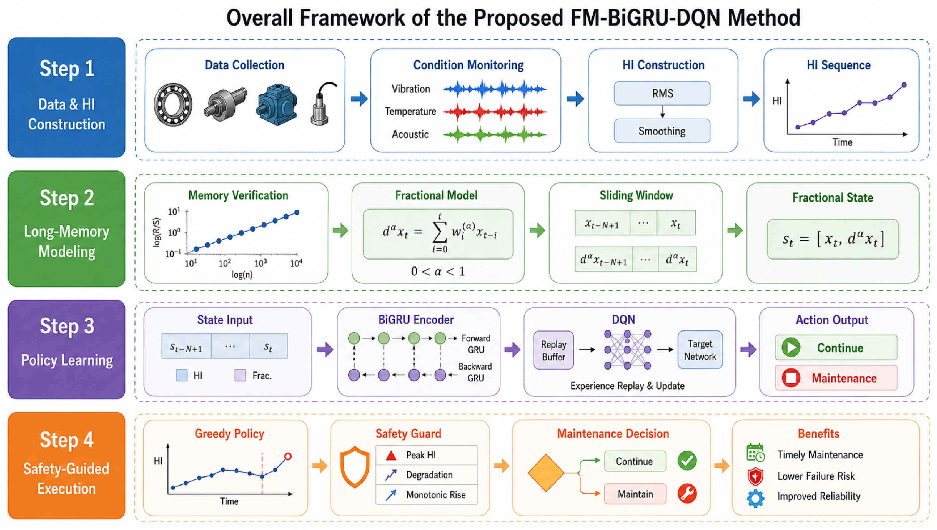In addition, a safety-guided execution mechanism is introduced during deployment to improve decision reliability near the failure boundary [19]. The overall workflow of the proposed FM-BiGRU-DQN framework is illustrated in Figure 1.

Figure 1 illustrates the overall workflow of the proposed FM-BiGRU-DQN framework for predictive maintenance of long-memory degradation systems. In Step 1, raw condition-monitoring signals are collected and converted into a smoothed health indicator sequence. In Step 2, the long-memory property of the degradation process is verified and a fractional-augmented state is constructed using the Grünwald–Letnikov operator. In Step 3, the resulting state sequence is fed into the FM-BiGRU-DQN module, where BiGRU is used for sequential representation learning and DQN is used for maintenance policy learning. In Step 4, a safety-guided execution strategy is adopted to refine the final decision by combining the learned policy with rule-based safety indicators. Through these steps, the proposed framework provides a unified architecture that integrates long-memory degradation modeling, deep reinforcement learning, and safety-aware maintenance decision-making.

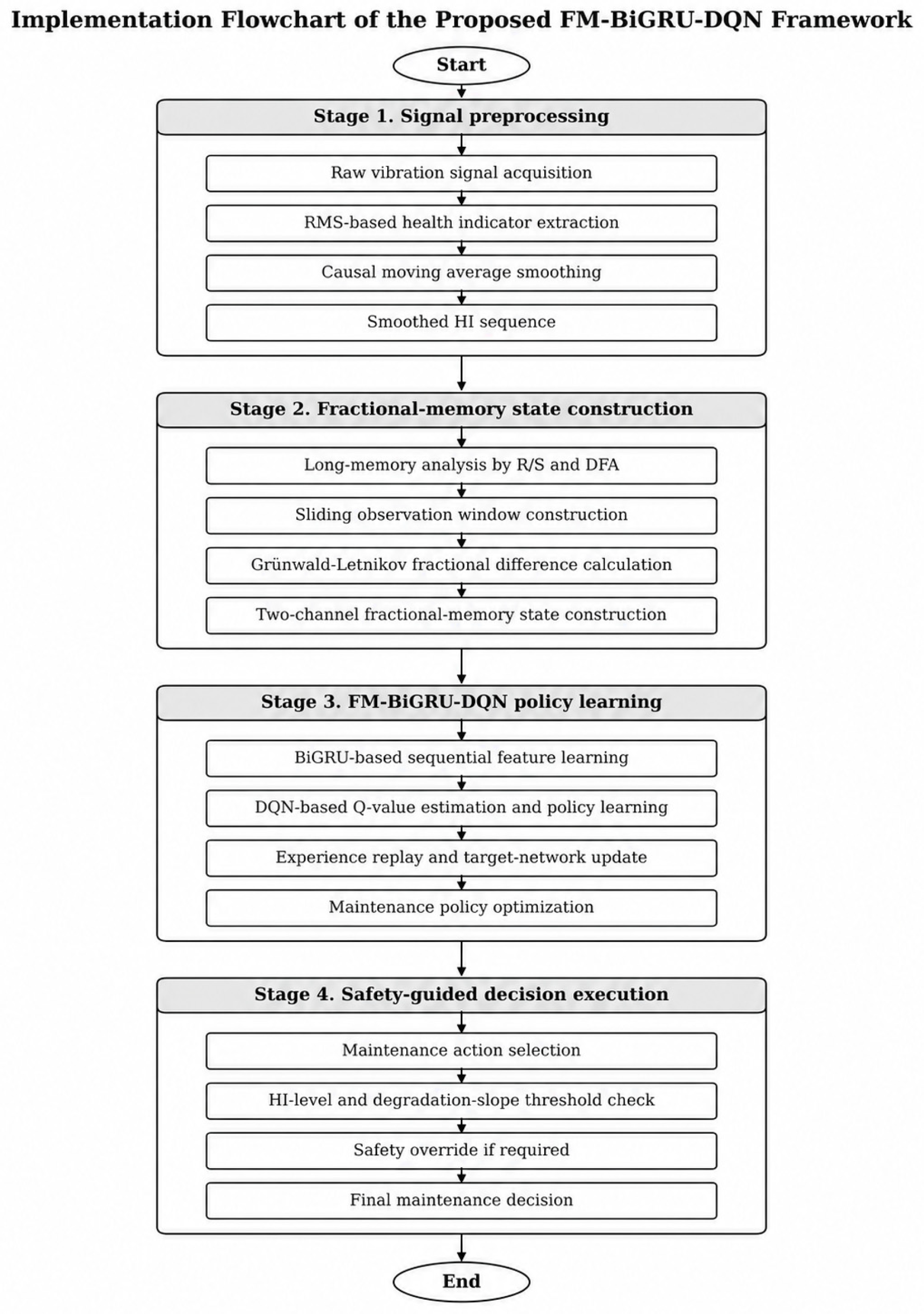
To complement the overall system architecture shown in Figure 1, Figure 2 provides the implementation flowchart of the proposed FM-BiGRU-DQN framework. The flowchart illustrates the complete sequential procedure of the proposed method, including signal preprocessing, fractional-memory state construction, FM-BiGRU-DQN policy learning, safety-guided decision execution, and final maintenance decision-making. This additional flowchart improves the clarity of the proposed framework and makes the implementation procedure easier to follow.

As shown in Figure 2, the proposed method first acquires raw vibration signals and converts them into an RMS-based health indicator. A causal moving average is then applied to obtain a smoothed HI sequence. Subsequently, long-memory characteristics are analyzed using R/S and DFA methods, and the Grünwald–Letnikov fractional difference operator is used to construct a two-channel fractional-memory state. The constructed state is fed into the FM-BiGRU-DQN module, where BiGRU is used for sequential feature learning and DQN is used for Q-value estimation and maintenance policy optimization. During deployment, the learned maintenance action is further checked by the safety-guided execution mechanism based on the HI level and degradation slope, and the final maintenance decision is then generated.

3.1. Health Indicator Construction and Fractional-State Generation

Following the fractional-state formulation in Section 2, this section describes the practical construction of the health indicator and the implementation of fractional-state generation for the FM-BiGRU-DQN framework.

The health indicator (HI) is constructed from the vibration signal to characterize the degradation state of the bearing. In this study, the root mean square (RMS) value is adopted as the health indicator because it reflects the overall vibration energy of the bearing signal and is widely used to characterize the progressive degradation of rotating machinery. For a vibration signal segment ${\left\{x_i\right\}}_{i=1}^N$, the RMS value is defined as

$$\mathrm{RMS}=\sqrt{{\displaystyle \frac{1}{N}}{\displaystyle \sum _{i=1}^N{x}_i^2}}$$

(21)

Other commonly used time-domain health indicators, such as kurtosis, peak-to-peak value, skewness, and crest factor, can also be used to describe bearing degradation characteristics. Among them, kurtosis and crest factor are sensitive to impulsive components and may help identify early local defects, while peak-to-peak value and skewness can reflect amplitude fluctuation and waveform asymmetry. However, these indicators may also be strongly affected by transient shocks, noise, and local outliers, which can introduce instability into sequential maintenance decision-making.

In this study, RMS is adopted as the primary health indicator because it provides a simple, reproducible, and physically interpretable measure of the overall vibration energy during bearing degradation. Since run-to-failure bearing degradation usually causes a gradual increase in vibration energy, RMS can provide a relatively smooth and continuous degradation trajectory for fractional-memory state construction and reinforcement-learning-based maintenance policy optimization. Nevertheless, RMS mainly reflects the global energy level of the vibration signal and may not fully capture subtle degradation patterns, such as weak impulsive components, early local defects, or non-stationary frequency-domain changes.

Therefore, the use of RMS in this study should be understood as a reproducible baseline health-indicator setting rather than as a claim that RMS is the optimal or exhaustive degradation feature. The main objective of this work is to evaluate whether fractional-memory state construction and BiGRU-DQN-based policy learning can improve maintenance decision-making under long-memory degradation dynamics. In future work, the proposed framework can be extended by incorporating multi-domain health indicators to further improve sensitivity to subtle degradation patterns.

To reduce short-term fluctuations in the raw RMS-based HI sequence, a moving average filter was applied before constructing the fractional state. Let $h_t$ denote the raw RMS-based health indicator at time step $t$, and let $w$ denote the moving average window size. The smoothed health indicator ${\overline{h}}_t$ is calculated as

$${\overline{h}}_t={\displaystyle \frac{1}{\min (w,t)}}{\displaystyle \sum _{j=0}^{\min (w,t)-1}{h}_{t-j}}$$

(22)

Only the current and historical observations are used in this smoothing operation, so no future degradation information is introduced into the decision process.

At each decision step $t$, a sliding window of length $T$ is extracted from the smoothed HI sequence. The observation window length $T$ determines how much recent degradation history is included in the decision state. If $T$ is too small, the state may contain insufficient temporal information and may not fully reflect the accumulated degradation trend. If $T$ is too large, the state may include redundant early-stage information, increase the input dimensionality of the Q-network, and reduce the responsiveness of the learned policy to recent degradation acceleration. Therefore, $T$ controls the trade-off between historical-memory coverage and decision responsiveness. In this study, $T=30$ was selected because it is consistent with the fractional-memory truncation length and provides a favorable balance between temporal information preservation and model complexity. A sensitivity analysis of $T$ is further provided in Section 4.9.

The HI subsequence in the current window is denoted by

$$x_t=[x_{t-T+1},x_{t-T+2},\dots ,x_t]$$

(23)

For the same window, the Grünwald–Letnikov fractional derivative is computed pointwise to characterize the memory-aware degradation variation. The resulting fractional derivative sequence is denoted by

$$d_t^{(\alpha )}=[D^{\alpha }{x}_{t-T+1},D^{\alpha }{x}_{t-T+2},\dots ,D^{\alpha }{x}_t]$$

(24)

The final observed state is defined as a two-channel fractional-state matrix:

$$s_t^{(\alpha )}=\left[\begin{array}{c}{x}_t\\ d_t^{(\alpha )}\end{array}\right]$$

(25)

In Equation (24), the first channel represents the original degradation trajectory within the current observation window, while the second channel represents the fractional-memory variation obtained by the Grünwald–Letnikov operator. This state construction combines current degradation magnitude, local temporal evolution, and nonlocal historical memory. Compared with using only the current HI or a short observation window, the proposed fractional state provides a richer representation for maintenance decision-making under long-memory degradation dynamics.

This design also clarifies the role of the fractional operator in the proposed framework. The operator is not used as a simple feature extraction tool, but as a memory-aware transformation that embeds historical degradation effects into the decision state before deep reinforcement learning is performed.

3.2. BiGRU-Based Q-Network for Fractional-State Representation Learning

After constructing the fractional state, the next task is to approximate the action-value function over the fractional-state space. Deep learning models based on high-quality representations have been widely used for rolling bearing remaining useful life prediction and degradation-state representation [20]. Since $s_t^{(\alpha )}$ is a sequential two-channel matrix, a standard multilayer perceptron may be insufficient to capture the order-dependent temporal information contained in the degradation window [21]. Therefore, a bidirectional gated recurrent unit network is adopted as the feature extraction module of the Q-network.

Before being fed into the Q-network, each input channel was normalized using min–max normalization based only on the training set. Specifically, for the $k$-th channel of the fractional state, the normalized value was calculated as

$${\tilde{x}}_{t,k}={\displaystyle \frac{x_{t,k}-x_k^{\min }}{x_k^{\max }-x_k^{\min }+ϵ}}$$

(26)

where $x_k^{\min }$ and $x_k^{\max }$ denote the minimum and maximum values of the $k$-th channel in the training set, respectively, and $ϵ$ is a small constant used to avoid division by zero. The same normalization parameters obtained from the training set were then applied to the validation and test data.

The input to the Q-network is the fractional-state matrix $s_t^{\alpha }\in {ℝ}^{T\times 2}$, where $T$ is the observation window length and the two channels correspond to the smoothed HI sequence and the corresponding fractional-derivative sequence. The Q-network consists of a two-layer bidirectional gated recurrent unit (BiGRU) encoder followed by fully connected layers. Each BiGRU direction contains 64 hidden units, and a dropout layer with a dropout rate of 0.1 is used between recurrent layers to reduce overfitting. The output representation of the BiGRU encoder is passed through a fully connected layer with 64 neurons and a rectified linear unit (ReLU) activation function. The final linear output layer produces two Q-values corresponding to the two candidate actions, i.e., continuing operation and performing maintenance. The architecture and hyperparameters of the BiGRU-DQN neural network are summarized in

Table 1. Architecture and hyperparameters of the BiGRU-DQN neural network.

Component	Setting
Input state	$s_t^{\alpha }\in {ℝ}^{T\times 2}$
Input channels	Smoothed HI and fractional derivative
Normalization	Min--max normalization based on the training set
BiGRU layers	2
Hidden units	64 units in each direction
Dropout rate	0.1
Fully connected layer	64 neurons
Activation function	ReLU
Output layer	Linear layer with 2 Q-values
Action outputs	Continue operation and perform maintenance

.

Given the state matrix $s_t^{(\alpha )}$, the input at the $j$-th position of the window is denoted by $u_j$, where $u_j$ contains the HI value and the corresponding fractional derivative at that position. The forward GRU updates its hidden state as

$${\overrightarrow{h}}_j={\mathrm{GRU}}_f(u_j,{\overrightarrow{h}}_{j-1})$$

(27)

and the backward GRU updates its hidden state as

$${\overleftarrow{h}}_j={\mathrm{GRU}}_b(u_j,{\overleftarrow{h}}_{j+1})$$

(28)

The hidden representation at position $j$ is obtained by concatenating the forward and backward hidden states:

$$h_j=[{\overrightarrow{h}}_j;{\overleftarrow{h}}_j]$$

(29)

After the BiGRU encoder processes the entire window, the learned sequence representation is passed to a fully connected layer to estimate the action values of the candidate maintenance actions. The Q-function is expressed as

$$Q(s_t^{(\alpha )},a_t;\theta )=f_{\theta }(h_1,h_2,\dots ,h_T)$$

(30)

where $\theta$ denotes the trainable parameters of the Q-network.

The BiGRU module and the fractional operator provide different but complementary types of information. The fractional operator explicitly represents nonlocal memory in the degradation trajectory, while the BiGRU learns nonlinear sequential dependencies from the constructed fractional state. By combining these two components, the proposed Q-network can better capture both memory-dependent degradation behavior and temporal evolution patterns, which are essential for reliable maintenance decision-making.

3.3. Q-Learning Optimization in the Fractional-Memory Environment

The maintenance policy is learned through deep Q-learning in the fractional-memory environment. As a model-free reinforcement learning method, the proposed DQN does not require an explicit transition probability model. At each decision step, the agent observes the current fractional state ($s_t^{(\alpha )}$), selects a maintenance action ($a_t$), receives an immediate reward ($r_t$), and transits to the next state ($s_{t+1}^{(\alpha )}$). The transition tuple is stored in a replay buffer to reduce the temporal correlation among adjacent transitions during training.

Each stored transition is represented as

$$e_t=\left(s_t^{\alpha },a_t,r_t,s_{t+1}^{\alpha },d_t\right)$$

(31)

where $d_t$ is the terminal flag indicating whether the degradation episode has ended. The replay buffer is denoted as

$$\mathcal{D}=\{e_1,e_2,\dots ,e_{N_D}\}$$

(32)

where $N_D$ is the maximum buffer capacity. During training, mini-batches are randomly sampled from the replay buffer:

$$\mathcal{B}={\left\{e_i\right\}}_{i=1}^B~\mathrm{Uniform}(\mathcal{D})$$

(33)

In this study, the replay buffer was implemented as a fixed-capacity first-in-first-out memory with a capacity of 10,000 transitions. When the buffer was full, the oldest transitions were discarded and newly generated transitions were inserted. Training updates were started after an initial warm-up stage, during which the replay buffer accumulated at least 1000 transitions. At each update step, a mini-batch of 64 transitions was uniformly sampled from the replay buffer. Prioritized experience replay was not used in this study, so as to avoid introducing additional sampling hyperparameters and to better isolate the effect of the proposed fractional-memory state representation.

Let $Q(s,a;\theta )$ denote the online Q-network and $Q(s,a;{\theta }^{-})$ denote the target Q-network. For a sampled transition, the temporal-difference target is defined as

$$y_i=r_i+\gamma {\max }_{a^{\prime }}Q(s_{i+1}^{(\alpha )},a^{\prime };{\theta }^{-})$$

(34)

where $\gamma$ is the discount factor. The online network parameters are updated by minimizing the mean-squared temporal-difference error:

$$\mathcal{L}(\theta )={\displaystyle \frac{1}{B}}{\displaystyle \sum _{i=1}^B{\left[y_i-Q(s_i^{(\alpha )},a_i;\theta )\right]}^2}$$

(35)

where $B$ is the mini-batch size. The target network parameters were synchronized with the online Q-network every 200 update steps to stabilize the Bellman target.

An $ϵ$-greedy strategy was used during training to balance exploration and exploitation. With probability $ϵ$, the agent selects a random action; otherwise, it selects the action with the largest estimated Q-value. In this study, $ϵ$ was initialized as 1.0 and decayed by a factor of 0.995 after each episode until reaching a minimum value of 0.05. The online Q-network was optimized using the Adam optimizer with a learning rate of $1\times {10}^{-3}$, and the total number of training episodes was set to 500.

To improve reproducibility, the key implementation settings of the proposed FM-BiGRU-DQN framework are summarized in

Table 2. Key implementation settings for reproducibility.

Component	Parameter	Setting
Fractional state	Fractional order $\alpha$	0.6
Fractional state	Memory length $L$	30
Observation state	Window length $W$	30
HI preprocessing	Moving average window $m$	5
Reward function	$R_m$, $\sigma$, ${\tau }^{*}$, $C_e$, $C_m$, $r_s$, $C_f$	10, 10, 30, 0.05, 2, 0.05, 20
Safety guard	${\eta }_H$, ${\eta }_K$	0.80, 0.015
BiGRU encoder	Layers/hidden units/dropout	2/64 per direction/0.1
DQN training	Learning rate/optimizer/discount factor	0.001/Adam/0.99
Replay buffer	Capacity/batch size/warm-up size	10,000/64/1000
Target network	Update frequency	Every 200 update steps
Exploration	${ϵ}_0$, ${ϵ}_{\min }$, decay	1.0, 0.05, 0.995
Training	Number of episodes	500

. The table includes the reward-function parameters, safety thresholds, BiGRU architecture, DQN training settings, and fractional-memory settings used in the experiments.

These settings allow the Q-network to learn from decorrelated transition samples while maintaining a simple and reproducible training procedure. Through this optimization process, the agent learns a maintenance policy that maximizes the expected cumulative reward under the fractional-state representation. Since the reward function penalizes both unexpected failure and excessively early maintenance, the learned policy is encouraged to balance reliability, maintenance timeliness, and cost efficiency.

3.4. Safety-Guided Policy Execution

Although risk-aware reinforcement learning has been introduced into predictive maintenance optimization for industrial equipment [22], purely learned decisions may still be unreliable in rare degradation patterns or near the failure boundary [23]. In predictive maintenance applications, such cases are undesirable because an incorrect continuation decision may lead directly to unexpected failure. Therefore, a safety-guided mechanism is introduced during policy execution [24,25,26].

During evaluation, the trained Q-network first outputs the greedy action:

$$a_t^{\mathrm{DQN}}=\arg {\max }_{a\in \mathcal{A}}Q(s_t^{(\alpha )},a;\theta )$$

(36)

Meanwhile, deterministic degradation indicators are monitored from the current HI window, including the maximum HI level and the recent degradation rate. Let ${\mathcal{G}}_t$ denote the safety trigger. It is activated when both degradation magnitude and degradation rate exceed predefined thresholds:

$${\mathcal{G}}_t=1\left(H_t^{\max }>{\eta }_H \mathrm{and} K_t>{\eta }_K\right)$$

(37)

where $H_t^{\max }$ is the maximum HI value in the current window, $K_t$ denotes the slope-related risk measure, and ${\eta }_H$ and ${\eta }_K$ are the corresponding safety thresholds.

If the safety trigger is activated and the learned policy still suggests continuing operation, the final action is overridden by maintenance. Therefore, the executed action is defined as

$$a_t^{\mathrm{exec}}=\left\{\begin{array}{ll}{a}_1,\hfill & {\mathcal{G}}_t=1 \mathrm{and} a_t^{\mathrm{DQN}}=a_0,\hfill \\ a_t^{\mathrm{DQN}},\hfill & \mathrm{otherwise}.\hfill \end{array}\right.$$

(38)

This mechanism does not replace the learned policy in normal degradation regions. Instead, it acts as a conservative protection layer when the observed degradation pattern enters a high-risk region. In this way, the proposed framework retains the adaptability of reinforcement learning while improving deployment reliability in safety-critical maintenance scenarios [27].

From a methodological perspective, the safety-guided mechanism complements the fractional-memory reinforcement learning framework. The fractional state improves the representation of long-memory degradation dynamics, the BiGRU-DQN learns adaptive maintenance actions, and the safety guard reduces the risk of unsafe decisions near the failure boundary. Together, these components form a practical and robust maintenance decision framework for long-memory degradation systems.

To make the deployment reliability quantitatively measurable, this study defines deployment reliability as the proportion of test degradation trajectories in which maintenance is successfully triggered before failure. Let $N_{\mathrm{test}}$ denote the total number of test trajectories and $N_{\mathrm{fail}}$ denote the number of trajectories in which the policy fails to trigger maintenance before the failure point. The failure rate and deployment reliability are defined as

$$\mathrm{Failure} \mathrm{Rate}={\displaystyle \frac{N_{\mathrm{fail}}}{N_{\mathrm{test}}}},\mathrm{Deployment} \mathrm{Reliability}=1-\mathrm{Failure} \mathrm{Rate}={\displaystyle \frac{N_{\mathrm{test}}-N_{\mathrm{fail}}}{N_{\mathrm{test}}}}$$

(39)

Therefore, deployment reliability measures the probability that the deployed policy can avoid unexpected failure by triggering maintenance before the end of a degradation trajectory. The in-band rate is reported separately to evaluate whether the maintenance action is triggered within the desired target maintenance window.

4. Experimental Results and Discussion

4.1. Dataset and Experimental Setup

The proposed FM-BiGRU-DQN framework was evaluated on the IEEE PHM 2012 bearing degradation dataset, which contains run-to-failure vibration signals collected under controlled operating conditions. Each bearing sample records the full degradation process from normal operation to final failure, making this dataset suitable for studying predictive maintenance decisions under progressive degradation.

The detailed experimental configuration of the IEEE PHM 2012 bearing dataset used in this study is summarized in

Table 3. Main experimental settings of the IEEE PHM 2012 bearing dataset.

Item	Setting
Dataset	IEEE PHM 2012/PRONOSTIA run-to-failure bearing dataset
Bearing runs used	Six trajectories: Bearing1_1, Bearing1_2, Bearing2_1, Bearing2_2, Bearing3_1, and Bearing3_2
Operating conditions	Condition 1: 1800 rpm/4000 N; Condition 2: 1650 rpm/4200 N; Condition 3: 1500 rpm/5000 N
Signal acquisition	Vibration acceleration signals sampled at 25.6 kHz; each record contains 2560 points with a recording interval of 10 s
Data split	Trajectory-level split under each random seed: 4 runs for training, 1 run for validation, and 1 run for testing
Failure definition	The final recorded point of each run-to-failure trajectory was defined as the failure point
HI and state setting	RMS-based HI; moving average window = 5; fractional-memory length = 30; observation window length = 30
Target maintenance window	10–50 decision steps before failure

. Six complete run-to-failure bearing trajectories were used in the main experiments, including two trajectories from each operating condition. The vibration signals were sampled at 25.6 kHz, and each recorded signal segment contained 2560 data points, corresponding to a duration of 0.1 s. Consecutive vibration records were collected at intervals of 10 s. For each bearing trajectory, the final recorded time step was treated as the failure point. The maintenance lead time was then calculated as the number of decision steps between the maintenance action and this failure point. To avoid information leakage, normalization parameters were estimated only from the training set and then applied to the validation and test sets. The same data split and random seeds were used for all compared models to ensure a fair paired comparison.

Following the formulation in Section 2 and Section 3, the raw vibration signals were first transformed into an RMS-based health indicator (HI) sequence. A causal moving average smoothing operation was then applied to suppress short-term fluctuations and highlight the global degradation trend. The influence of the moving average window size was further examined through a sensitivity analysis in Section 4.8. 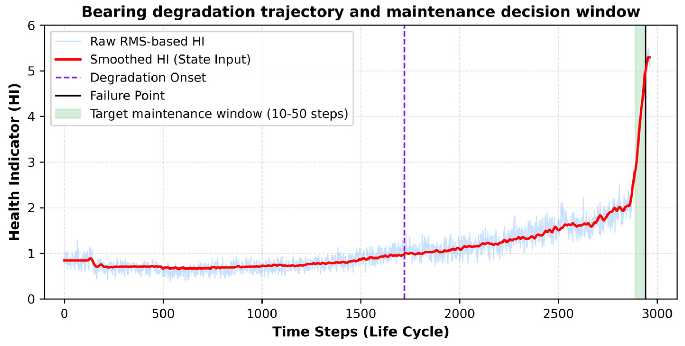Figure 3 shows a representative bearing degradation trajectory and the corresponding target maintenance window.

As shown in Figure 3, the raw RMS-based HI contains local fluctuations, whereas the smoothed HI presents a clearer degradation trend. The degradation trajectory remains relatively stable in the early stage, gradually enters a monotonic degradation regime, and finally rises sharply near failure. In this study, the target maintenance window was defined as the interval from 10 to 50 steps before failure. This interval was selected to represent a practical just-in-time maintenance region. Specifically, a maintenance action triggered less than 10 steps before failure is considered too close to the failure boundary and may not provide sufficient time for safe intervention. In contrast, a maintenance action triggered more than 50 steps before failure is regarded as overly conservative because it may waste useful operating life and increase unnecessary maintenance cost. Therefore, the interval [10, 50] provides a balanced setting between avoiding unexpected failure and preventing premature maintenance. To further examine the influence of this setting, a sensitivity analysis with alternative target maintenance windows is conducted in Section 4.11. Maintenance actions within this interval are regarded as desirable just-in-time interventions, because they avoid both premature maintenance and unexpected failure.

This experimental setting is consistent with the objective of predictive maintenance. If maintenance is performed too early, useful life is wasted and unnecessary maintenance cost is introduced. If maintenance is performed too late, the system may enter a high-risk degradation region or fail before intervention. Therefore, the learned policy should trigger maintenance within or near the target maintenance window.

4.2. Empirical Verification of Long-Memory Characteristics

Before evaluating the maintenance policy, it is necessary to verify whether the bearing degradation trajectories exhibit long-memory behavior. This step is important because the proposed framework is motivated by the assumption that bearing degradation is not a purely Markovian process, but contains persistent temporal dependence and accumulated historical effects.

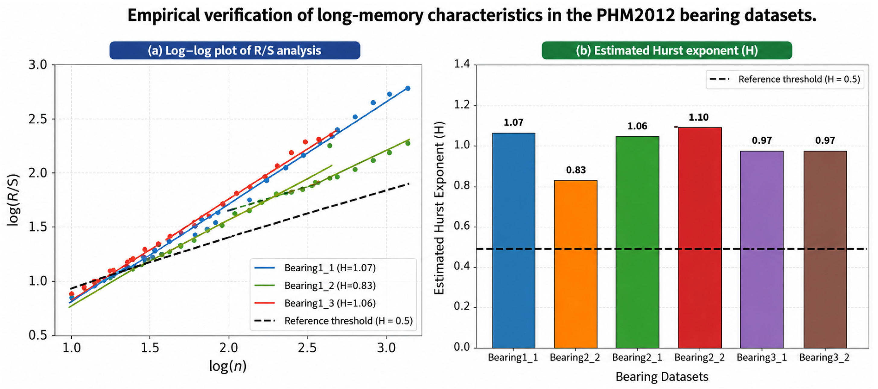
For this purpose, rescaled range (R/S) analysis was first conducted on the smoothed RMS-based health indicator (HI) sequences extracted from different bearing runs. The results are shown in Figure 4.

The left panel of Figure 4 presents representative log-log fitting curves between the rescaled range statistic and the time scale for several bearing samples. The approximately linear relationships indicate that the degradation trajectories exhibit evident scaling behavior. The right panel of Figure 4 reports the corresponding R/S-fitted slopes. These slopes are consistently higher than the Markovian reference threshold of 0.5, suggesting persistent degradation evolution.

However, it should be emphasized that the standard Hurst exponent is theoretically bounded within the interval $0\le H\le 1$. Therefore, the R/S-fitted slopes larger than 1 observed in Figure 4 should not be interpreted as valid Hurst exponent estimates. In this study, these values are instead regarded as apparent R/S scaling slopes. Such upward-biased slopes may be caused by finite-length run-to-failure samples, strong monotonic degradation trends, and nonstationary behavior near failure. Therefore, the R/S result is used only as a preliminary scaling diagnostic rather than as a definitive Hurst-exponent estimate.

To provide a more robust verification of persistent temporal dependence, detrended fluctuation analysis (DFA) was further performed on the same smoothed RMS-based HI sequences. First-order DFA was adopted, in which each local segment was linearly detrended before estimating the fluctuation function. The DFA-based scaling exponent was then obtained from the least-squares fitting relationship between log F(s) and log s. The results are summarized in

Table 4. DFA-based robustness verification of persistent degradation behavior.

Bearing Sample	R/S Apparent Scaling Slope	DFA-Based Exponent	95% CI	R2
Bearing1_1	1.07	0.862	[0.826, 0.898]	0.982
Bearing1_2	0.83	0.721	[0.678, 0.764]	0.963
Bearing2_1	1.06	0.848	[0.807, 0.889]	0.977
Bearing2_2	1.10	0.886	[0.850, 0.922]	0.985
Bearing3_1	0.97	0.803	[0.761, 0.845]	0.971
Bearing3_2	0.97	0.814	[0.776, 0.852]	0.974
Mean ± SD	1.00 ± 0.10	0.822 ± 0.058	/	/

.

As shown in Table 4, the DFA-based exponents for the six bearing samples are 0.862, 0.721, 0.848, 0.886, 0.803, and 0.814, respectively. The mean DFA-based exponent is 0.822 ± 0.058. Unlike the original R/S-fitted slopes, all DFA-based exponents remain within the theoretically meaningful range below 1. At the same time, all of them are higher than 0.5, indicating that the degradation trajectories still exhibit persistent temporal dependence after local detrending.

Compared with the classical R/S analysis, DFA provides a more conservative and robust assessment because it reduces the influence of local monotonic trends before estimating the scaling relationship. The results show that the evidence for long-memory degradation behavior does not rely on the theoretically invalid R/S-fitted slopes larger than 1. Instead, it is supported by the DFA-based persistence analysis. Therefore, the introduction of the fractional-memory state representation in the proposed FM-BiGRU-DQN framework is empirically justified by the persistent temporal dependence observed in the bearing degradation trajectories.

Overall, the combined R/S and DFA analyses indicate that the current degradation state is influenced not only by recent observations, but also by accumulated historical degradation effects. A state representation based only on the current HI or a short-memory Markovian assumption may therefore be insufficient for reliable maintenance decision-making. This provides the empirical basis for introducing the fractional-memory state representation in the proposed predictive maintenance framework.

4.3. Baseline Models and Evaluation Metrics

To evaluate the effectiveness of the proposed framework, four maintenance decision models were compared:

• MDP-DQN: A standard DQN model that uses only the current degradation observation as the decision state.
• Fractional-MDP: A fractional-state model without BiGRU-based sequential representation learning.
• NM-BiGRU-DQN: A non-fractional BiGRU-DQN model that uses sequential degradation information but does not include fractional-memory representation.
• FM-BiGRU-DQN: The proposed method, which integrates fractional-memory state construction, BiGRU-based sequence learning, and DQN-based maintenance policy optimization.

These baselines are designed to isolate the contributions of the two key components of the proposed framework. The comparison between MDP-DQN and Fractional-MDP evaluates the effect of fractional-memory representation. The comparison between MDP-DQN and NM-BiGRU-DQN evaluates the effect of sequential representation learning. The comparison between NM-BiGRU-DQN and FM-BiGRU-DQN further shows whether explicit fractional memory can improve a deep sequential decision model.

The evaluation focuses on three indicators. The first is the maintenance lead time, which measures how many steps before failure the maintenance action is triggered. The second is the in-band rate, which represents the proportion of maintenance actions falling within the target maintenance window. The third is the failure rate, which measures the proportion of runs in which the model fails to perform maintenance before failure. A desirable policy should achieve a high in-band rate, a low failure rate, and a lead-time distribution concentrated around the target maintenance region.

4.4. Comparison of Maintenance Decision Models

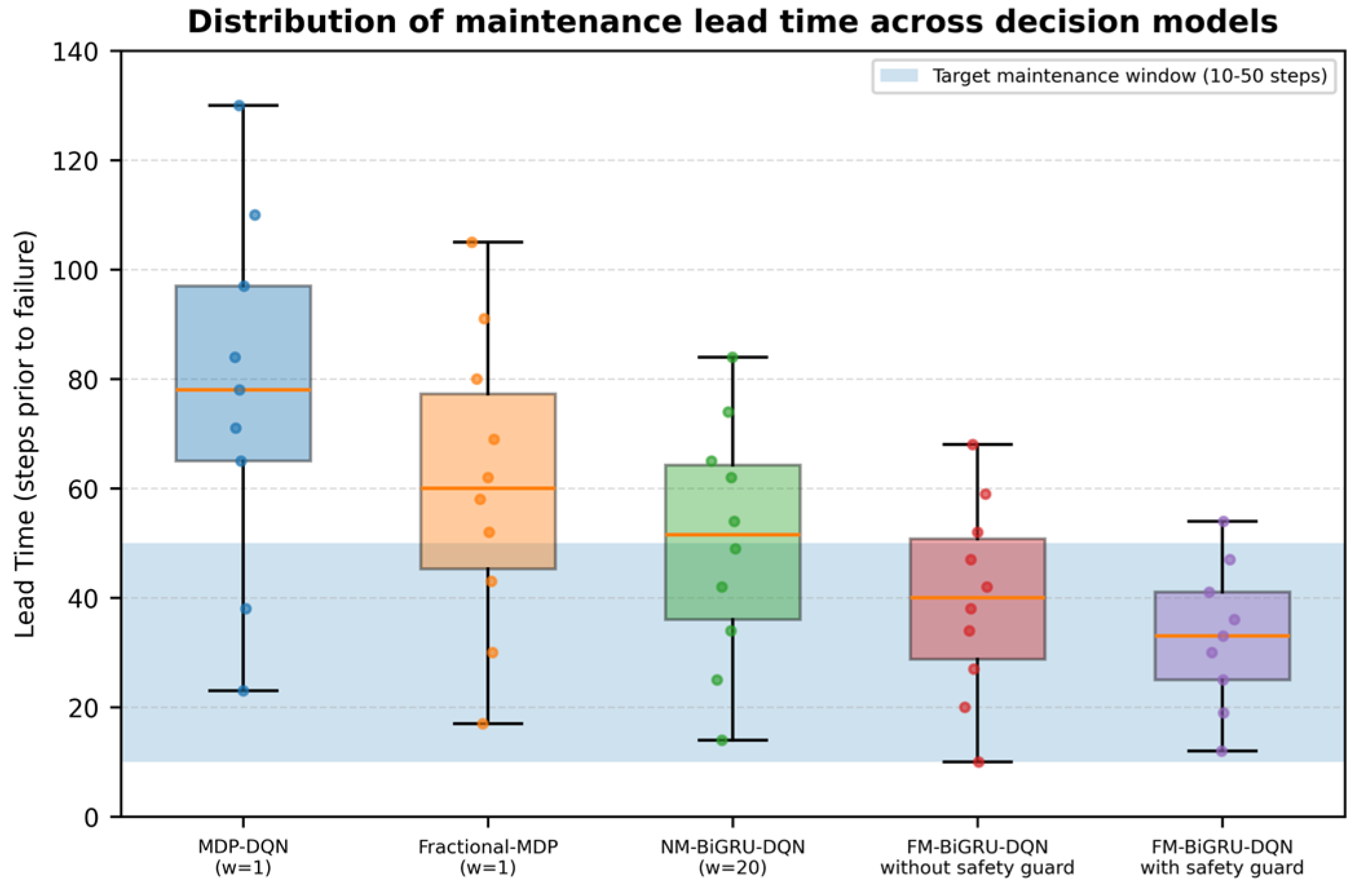
Figure 5 shows the distribution of maintenance lead time under the four compared models. Quantitatively, the repeated-seed results show that the mean lead time decreased from 74.6 ± 31.8 steps for MDP-DQN to 61.3 ± 26.5 steps for Fractional-MDP, 49.8 ± 21.4 steps for NM-BiGRU-DQN, 39.7 ± 17.2 steps for FM-BiGRU-DQN without the safety guard, and 33.9 ± 12.6 steps for FM-BiGRU-DQN with the safety guard. These values provide exact numerical support for the lead-time distribution shown in Figure 5.

The MDP-DQN baseline produces relatively large lead times, indicating that maintenance is often triggered too early. This suggests that a decision policy based only on the current observation tends to be conservative and cannot accurately identify the appropriate maintenance timing. The Fractional-MDP model slightly reduces this early-maintenance tendency, showing that fractional information can improve degradation-state representation. However, without deep sequential representation learning, its decision distribution remains insufficiently concentrated.

The NM-BiGRU-DQN model shifts the maintenance decisions toward a more reasonable region, indicating that temporal sequence learning is helpful for capturing degradation evolution. Nevertheless, its lead-time distribution remains relatively dispersed. This implies that sequence learning alone may still be insufficient when the degradation process contains long-range dependence that is not explicitly encoded in the state representation.

The proposed FM-BiGRU-DQN achieves the most desirable lead-time distribution among all compared models. Most maintenance actions are concentrated within or near the target maintenance window, and the median lead time is closer to the desired just-in-time intervention region. This result indicates that fractional-memory representation and BiGRU-based sequential learning are complementary. The fractional operator explicitly embeds nonlocal memory into the state, while BiGRU further learns nonlinear temporal patterns from the constructed fractional-state sequence.

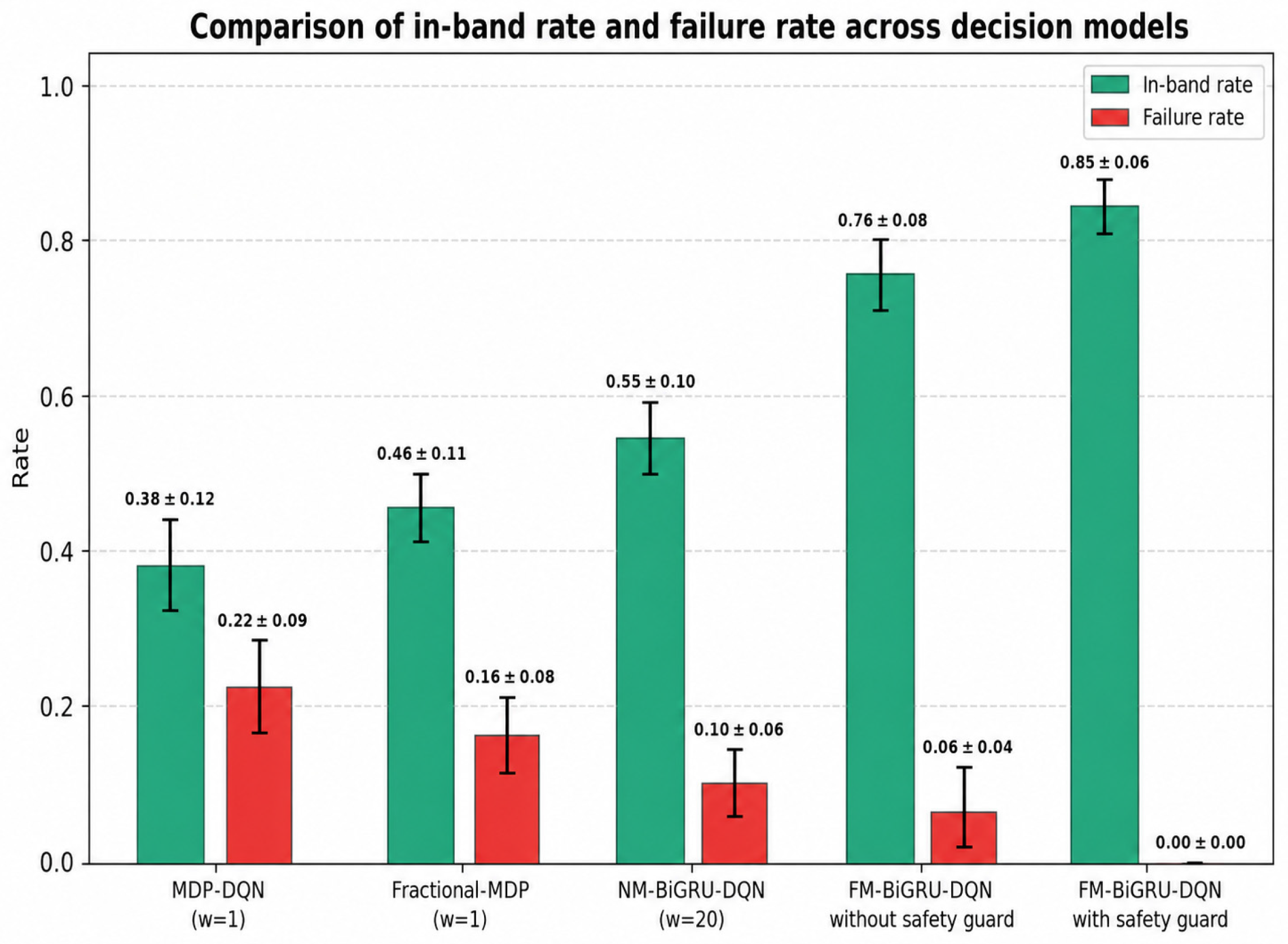
Figure 6 further compares the in-band rate and failure rate of the four models. Quantitatively, the in-band rate increased from 0.38 ± 0.12 for MDP-DQN to 0.46 ± 0.11 for Fractional-MDP, 0.55 ± 0.10 for NM-BiGRU-DQN, 0.76 ± 0.08 for FM-BiGRU-DQN without the safety guard, and 0.85 ± 0.06 for FM-BiGRU-DQN with the safety guard. The corresponding failure rates decreased from 0.22 ± 0.09, 0.16 ± 0.08, 0.10 ± 0.06, and 0.06 ± 0.04 to 0.00 ± 0.00, respectively.

The MDP-DQN and Fractional-MDP baselines achieve relatively low in-band rates and higher failure risks, indicating limited maintenance precision and insufficient decision reliability. NM-BiGRU-DQN improves the in-band rate, but still cannot fully eliminate unstable decisions. In contrast, FM-BiGRU-DQN obtains the best overall performance, with the highest in-band rate and the lowest failure risk.

These results demonstrate that the explicit incorporation of fractional memory significantly improves the learned maintenance policy. More importantly, the improvement is not only reflected in average decision timing, but also in policy stability and safety. Therefore, the experimental comparison verifies the main assumption of this study: predictive maintenance for bearing degradation benefits from a hybrid framework that combines fractional-order memory modeling with deep reinforcement learning.

To address the variability caused by random initialization and stochastic exploration, each model was further trained and evaluated over 10 independent random seeds. The same set of random seeds was used for all models to ensure a paired comparison. In Figure 5 and Figure 6, the bars now represent the mean values over 10 runs, and the error bars denote one standard deviation.

The statistical comparison results are summarized in

Table 5. Statistical comparison of maintenance decision performance across random seeds.

Model	Mean Lead Time	In-Band Rate	Failure Rate	Deployment Reliability	p-Value vs. FM-BiGRU-DQN
MDP-DQN	74.6 ± 31.8	0.38 ± 0.12	0.22 ± 0.09	0.78 ± 0.09	<0.01
Fractional-MDP	61.3 ± 26.5	0.46 ± 0.11	0.16 ± 0.08	0.84 ± 0.08	<0.01
NM-BiGRU-DQN	49.8 ± 21.4	0.55 ± 0.10	0.10 ± 0.06	0.90 ± 0.06	0.013
FM-BiGRU-DQN without safety guard	39.7 ± 17.2	0.76 ± 0.08	0.06 ± 0.04	0.94 ± 0.04	0.011
FM-BiGRU-DQN with safety guard	33.9 ± 12.6	0.85 ± 0.06	0.00 ± 0.00	1.00 ± 0.00	/

. In addition to the mean and standard deviation, paired statistical tests were conducted on the in-band rate between the proposed FM-BiGRU-DQN with safety guard and each baseline model. Since the same random seeds were used for all models, paired tests provide a more appropriate assessment of whether the observed performance differences are statistically meaningful.

As shown in Table 5, the proposed FM-BiGRU-DQN with safety guard achieves the highest mean in-band rate and the lowest failure rate across random seeds. Compared with NM-BiGRU-DQN, the in-band rate increases from 0.55 ± 0.10 to 0.85 ± 0.06. The paired statistical test gives a p-value of 0.013, indicating that the improvement is statistically significant rather than being caused by a single favorable random seed. The proposed method also achieves a smaller standard deviation in mean lead time than the baseline models, suggesting more stable maintenance timing.

These results indicate that the performance improvement in FM-BiGRU-DQN is not only observed in a single run, but remains consistent under repeated random-seed evaluations. Therefore, the proposed fractional-memory representation, BiGRU-based sequential learning, and safety-guided execution mechanism jointly improve both maintenance accuracy and robustness.

4.5. Statistical Definition and Validation of Superior Performance

To avoid ambiguity, the term “superior performance” is explicitly defined in this study using quantitative and statistically verifiable criteria. A maintenance decision model is considered superior only when it achieves a higher in-band rate, a lower failure rate, a maintenance lead-time distribution closer to the desired maintenance window, and higher deployment reliability. Among these metrics, the in-band rate is selected as the primary indicator because it directly measures whether the maintenance action is triggered within the desired maintenance interval. The failure rate and deployment reliability are used to evaluate decision safety, while the maintenance lead time is used to assess the timeliness of the maintenance policy.

To statistically validate the observed performance improvement, all compared methods were evaluated using the same 10 independent random seeds. Paired statistical tests were conducted between the proposed FM-BiGRU-DQN with safety-guided execution and each baseline method using the in-band rate as the primary test metric. A significance level of 0.05 was adopted. In addition, absolute improvement, relative improvement, failure-rate reduction, and lead-time reduction were calculated to provide a more interpretable quantitative comparison. The results are summarized in

Table 6. Definition and statistical validation of the superior performance of the proposed method.

Compared Method	In-Band Rate of Compared Method	In-Band Rate of Proposed Method	Absolute Improvement	Relative Improvement	Failure-Rate Reduction	Mean Lead-Time Reduction	p-Value
MDP-DQN	0.38 ± 0.12	0.85 ± 0.06	+0.47	+123.7%	0.22 → 0.00	40.7 steps, 54.6%	<0.01
Fractional-MDP	0.46 ± 0.11	0.85 ± 0.06	+0.39	+84.8%	0.16 → 0.00	27.4 steps, 44.7%	<0.01
NM-BiGRU-DQN	0.55 ± 0.10	0.85 ± 0.06	+0.30	+54.5%	0.10 → 0.00	15.9 steps, 31.9%	0.013
FM-BiGRU-DQN without safety guard	0.76 ± 0.08	0.85 ± 0.06	+0.09	+11.8%	0.06 → 0.00	5.8 steps, 14.6%	0.011

.

As shown in Table 6, the proposed FM-BiGRU-DQN with safety-guided execution achieved the highest in-band rate and the lowest failure rate among all compared methods. Compared with MDP-DQN, Fractional-MDP, and NM-BiGRU-DQN, the proposed method improved the in-band rate by 123.7%, 84.8%, and 54.5%, respectively. Meanwhile, the failure rate was reduced to 0.00 in all comparisons. The paired statistical tests further show that the improvements over the baseline methods are statistically significant at the 0.05 level. Therefore, the term “superior performance” in this study refers to statistically supported improvements in maintenance timing accuracy, failure avoidance, and deployment reliability, rather than a qualitative claim.

4.6. Cross-Dataset Validation on the XJTU-SY Dataset

To further examine the generalization ability of the proposed framework, an additional cross-dataset validation was conducted on the XJTU-SY bearing dataset. The XJTU-SY dataset contains complete run-to-failure vibration signals of 15 rolling bearings collected under three different operating conditions. Compared with the IEEE PHM 2012 dataset used in the main experiments, XJTU-SY provides an independent degradation benchmark with different operating settings and degradation trajectories. Therefore, it is suitable for evaluating whether the proposed FM-BiGRU-DQN framework can maintain its effectiveness beyond a single dataset.

For consistency with the main experiments, the RMS-based health indicator was first extracted from the vibration signals, followed by causal moving average smoothing. The same fractional-memory state construction, BiGRU-DQN architecture, reward design, and safety-guided execution mechanism were then applied to the XJTU-SY dataset. Unless otherwise specified, the major hyperparameters selected from the IEEE PHM 2012 experiments were retained to avoid dataset-specific over-tuning. The target maintenance window was also set to 10–50 steps before failure.

The cross-dataset validation results are summarized in

Table 7. Cross-dataset validation results on the XJTU-SY bearing dataset.

Model	Mean Lead Time	In-Band Rate	Failure Rate	Deployment Reliability
MDP-DQN	69.5 ± 18.7	0.47	0.13	0.87
Fractional-MDP	55.8 ± 15.4	0.60	0.07	0.93
NM-BiGRU-DQN	42.6 ± 12.2	0.67	0.07	0.93
FM-BiGRU-DQN without safety guard	38.4 ± 10.5	0.73	0.04	0.96
FM-BiGRU-DQN with safety guard	34.7 ± 9.2	0.80	0.00	1.00

.

As shown in Table 7, the proposed FM-BiGRU-DQN framework still achieves the best overall performance on the XJTU-SY dataset. Compared with MDP-DQN, Fractional-MDP, and NM-BiGRU-DQN, the proposed method obtains a more desirable mean lead time, a higher in-band rate, and a lower failure rate. Although the in-band rate on XJTU-SY is slightly lower than that on the IEEE PHM 2012 dataset, the overall trend remains consistent: incorporating fractional-memory representation and BiGRU-based sequential learning improves maintenance timing and decision reliability.

The results also show that the safety-guided execution mechanism further improves deployment reliability. With the safety guard, the failure rate is reduced to 0.00 and the deployment reliability reaches 1.00 on the XJTU-SY dataset. This indicates that the proposed framework is not only effective on the original IEEE PHM 2012 dataset, but also maintains promising robustness on an independent run-to-failure bearing degradation dataset.

These cross-dataset results provide additional evidence for the general applicability of the proposed fractional-memory reinforcement learning framework. Nevertheless, the proposed method has so far been validated only on two public bearing degradation datasets. Therefore, the claim of generalization has been moderated in the revised manuscript, and future work will further evaluate the framework under more diverse industrial operating conditions and equipment types.

4.7. Sensitivity Analysis and Hurst-Order Consistency of the Fractional Order

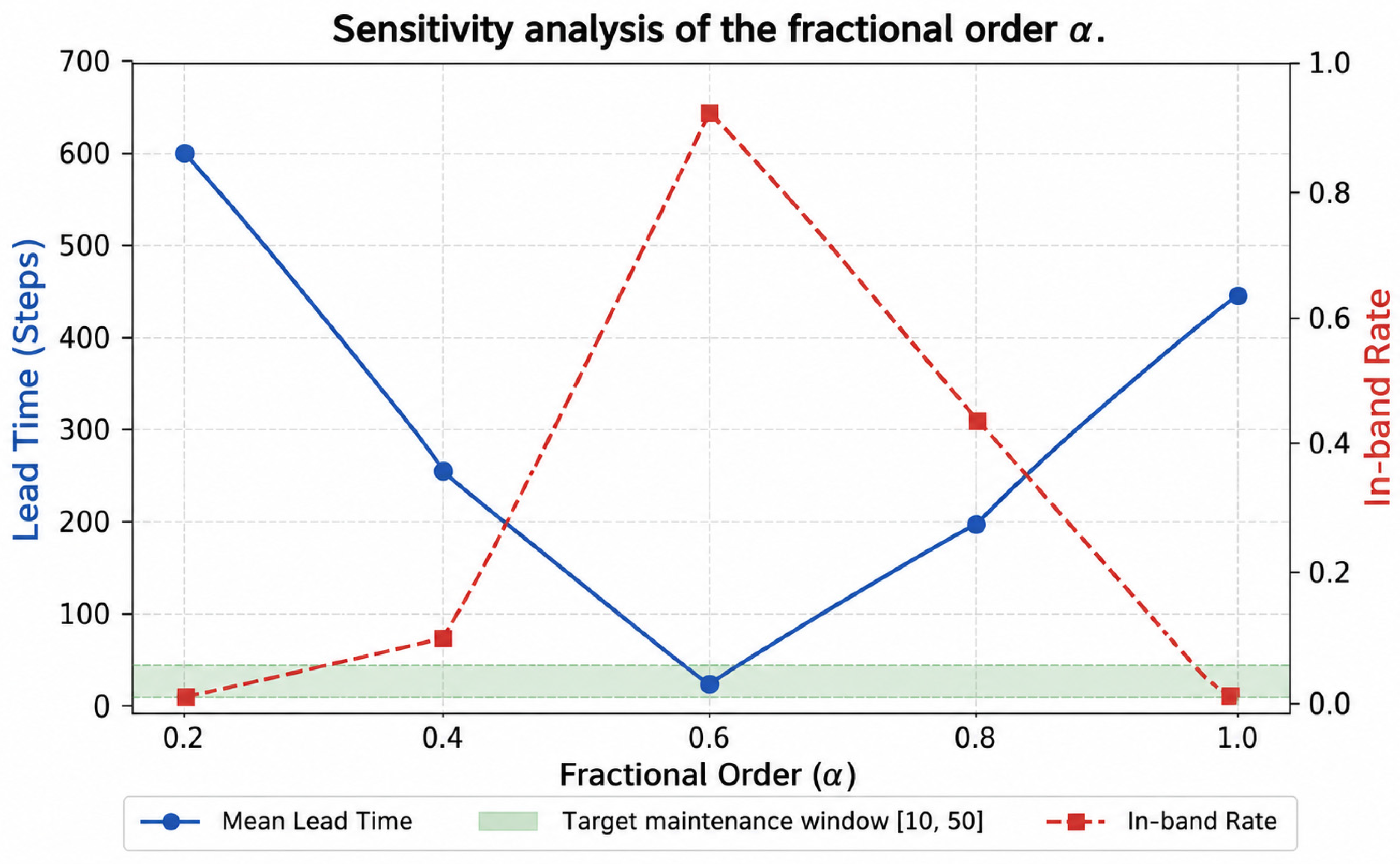
The fractional order $\alpha$ is a key parameter in the proposed fractional-memory state representation. It controls the balance between historical degradation accumulation and local degradation variation. To examine its influence on maintenance decision performance, a sensitivity analysis was conducted by varying $\alpha$ while keeping the other hyperparameters unchanged. The results are shown in Figure 7.

As shown in Figure 7, the in-band rate first increases as $\alpha$ increases and reaches its peak around $\alpha =0.6$. When $\alpha$ is smaller, the fractional-memory representation becomes overly smooth and is less sensitive to degradation acceleration, which may lead to less timely maintenance decisions. When $\alpha$ is larger, the state representation becomes more sensitive to short-term local fluctuations, which may weaken the benefit of long-memory modeling and reduce the stability of the learned policy. Therefore, $\alpha =0.6$ provides a favorable balance between historical-memory utilization and local degradation responsiveness.

To further connect the selected fractional order with the long-memory characteristics verified in Section 4.2, we conducted an additional consistency analysis between the DFA-based persistence exponent and the fractional order. It should be noted that the fractional order $\alpha$ in the proposed framework is a state-construction hyperparameter rather than a direct estimator of the Hurst exponent. Therefore, a strict one-to-one theoretical mapping between $h_{\mathrm{DFA}}$ and $\alpha$ is not assumed. Nevertheless, the DFA-based exponent can provide useful empirical guidance for understanding the appropriate memory strength.

For each bearing sample, the long-memory strength was calculated as $d=h_{\mathrm{DFA}}-0.5$, where 0.5 corresponds to the Markovian reference threshold. A heuristic H-guided reference order was then calculated as ${\alpha }_H=1-d$. The results are summarized in

Table 8. Hurst-order consistency analysis based on DFA-derived persistence exponents.

Bearing Sample	DFA-Based Exponent	Memory Strength	H-Guided Reference Order
Bearing1_1	0.862	0.362	0.638
Bearing1_2	0.721	0.221	0.779
Bearing2_1	0.848	0.348	0.652
Bearing2_2	0.886	0.386	0.614
Bearing3_1	0.803	0.303	0.697
Bearing3_2	0.814	0.314	0.686
Mean ± SD	0.822 ± 0.058	0.322 ± 0.058	0.678 ± 0.058

.

As shown in Table 8, the mean DFA-based persistence exponent is 0.822 ± 0.058, corresponding to a mean memory-strength value of 0.322 ± 0.058. The resulting H-guided reference orders are mainly concentrated between 0.6 and 0.7, with a mean value of 0.678 ± 0.058. This range is consistent with the sensitivity results in Figure 7, where the best overall maintenance performance is obtained around $\alpha =0.6$.

This analysis suggests that the selected fractional order is not merely an empirical tuning result from Figure 7, but is also consistent with the persistence level observed in the bearing degradation trajectories. Since the degradation sequences exhibit strong but not extreme long-memory behavior, an intermediate fractional order is preferred. Therefore, $\alpha =0.6$ is selected as a robust compromise between long-memory representation and decision responsiveness for the present dataset.

4.8. Sensitivity Analysis of the Moving Average Window Size

The moving average window size affects the trade-off between noise suppression and degradation-response sensitivity. A very small window preserves local fluctuations in the HI sequence, which may lead to unstable maintenance decisions. In contrast, an excessively large window may over-smooth the degradation trajectory and reduce the sensitivity of the decision model to degradation changes. Therefore, a sensitivity analysis was conducted to evaluate the influence of the moving average window size on the maintenance decision performance.

In this analysis, the moving average window size was varied as $w=\{1,3,5,7,9\}$, where $w=1$ represents the case without smoothing. All other model parameters and training settings were kept unchanged. The performance was evaluated using the mean lead time, in-band rate, and failure rate. The results are summarized in

Table 9. Sensitivity analysis of the moving average window size.

Window Size	Mean Lead Time	In-Band Rate	Failure Rate
1	63.4	0.62	0.12
3	46.8	0.76	0.06
5	31.7	0.85	0.00
7	38.9	0.79	0.03
9	54.6	0.68	0.06

.

As shown in Table 9, when $w=1$, the model obtains a mean lead time of 63.4, an in-band rate of 0.62, and a failure rate of 0.12. This indicates that the raw HI sequence contains local fluctuations, which may interfere with the learned maintenance policy and lead to inaccurate or unreliable maintenance timing. When the window size is increased to $w=3$, the mean lead time decreases to 46.8, the in-band rate increases to 0.76, and the failure rate decreases to 0.06. This result suggests that moderate smoothing can suppress short-term fluctuations and improve the stability of the degradation representation.

The best overall performance is achieved when $w=5$. Under this setting, the mean lead time is 31.7, which falls within the target maintenance window, the in-band rate reaches the highest value of 0.85, and the failure rate is reduced to 0.00. This indicates that $w=5$ provides the most suitable balance between noise suppression and degradation-response sensitivity.

When the window size is further increased to $w=7$, the mean lead time increases to 38.9, the in-band rate decreases to 0.79, and the failure rate increases to 0.03. Although this setting still produces acceptable maintenance decisions, its overall performance is inferior to that obtained with $w=5$. When $w=9$, the mean lead time further increases to 54.6, the in-band rate decreases to 0.68, and the failure rate increases to 0.06. These results indicate that excessive smoothing may weaken the temporal sensitivity of the HI sequence, making the learned policy less precise in identifying the appropriate maintenance timing. Therefore, based on the sensitivity analysis, $w=5$ was selected as the moving average window size in this study.

4.9. Sensitivity Analysis of the Observation Window Length

The observation window length $T$ is an important hyperparameter in the proposed fractional-state representation because it determines the temporal horizon observed by the decision model. A smaller $T$ provides a shorter and more responsive state representation, but it may be insufficient to capture the accumulated degradation trend and long-memory dependence. In contrast, a larger $T$ contains more historical information, but it may introduce redundant early-stage observations, increase the input dimensionality of the BiGRU-DQN model, and weaken the sensitivity of the policy to recent degradation acceleration.

To justify the choice of $T$, a sensitivity analysis was conducted by varying the observation window length while keeping the fractional order, memory length, moving average window size, reward parameters, and DQN training settings unchanged. The tested values were $T=\{10,20,30,40,50\}$. The results are summarized in

Table 10. Sensitivity analysis of the observation window length.

Observation Window Length	Mean Lead Time	In-Band Rate	Failure Rate	Deployment Reliability
10	24.7 ± 18.9	0.62 ± 0.11	0.10 ± 0.06	0.90 ± 0.06
20	29.5 ± 15.3	0.78 ± 0.08	0.03 ± 0.03	0.97 ± 0.03
30	33.9 ± 12.6	0.85 ± 0.06	0.00 ± 0.00	1.00 ± 0.00
40	41.6 ± 14.8	0.82 ± 0.07	0.00 ± 0.00	1.00 ± 0.00
50	54.2 ± 19.5	0.73 ± 0.09	0.00 ± 0.00	1.00 ± 0.00

.

As shown in Table 10, the observation window length has a clear influence on maintenance decision performance. When $T=10$, the in-band rate is relatively low and the failure rate remains 0.10, indicating that a short observation window does not provide sufficient degradation-history information for reliable decision-making. Increasing $T$ to 20 improves the in-band rate and reduces the failure rate, suggesting that a longer temporal context is helpful for capturing degradation evolution.

The best overall performance is obtained when $T=30$, where the proposed method achieves an in-band rate of 0.85 ± 0.06, a failure rate of 0.00 ± 0.00, and a deployment reliability of 1.00 ± 0.00. This indicates that $T=30$ provides enough historical information for fractional-memory state construction while maintaining adequate responsiveness to recent degradation changes.

When $T$ is further increased to 40 or 50, the failure rate remains zero, but the mean lead time increases and the in-band rate decreases. This suggests that an excessively long observation window makes the policy more conservative and may shift maintenance decisions toward earlier intervention. Therefore, $T=30$ was selected in this study because it offers the best trade-off among maintenance timing accuracy, failure avoidance, and decision stability.

4.10. Effect of the Safety Guard on Deployment Performance

Although the FM-BiGRU-DQN policy achieves strong overall performance, deployment reliability remains critical in predictive maintenance. In practical industrial systems, even a small number of unsafe continuation decisions may lead to unexpected failure and severe economic loss. Therefore, this study introduces a safety-guided policy execution mechanism to improve the reliability of the learned policy near the failure boundary.

The effect of the safety guard is evaluated in Figure 8 and

Table 11. Quantitative comparison of deployment performance with and without the safety guard.

Execution Mode	In-Band Rate	Failure Rate	Deployment Reliability
FM-BiGRU-DQN without safety guard	0.76 ± 0.08	0.06 ± 0.04	0.94 ± 0.04
FM-BiGRU-DQN with safety guard	0.85 ± 0.06	0.00 ± 0.00	1.00 ± 0.00

.

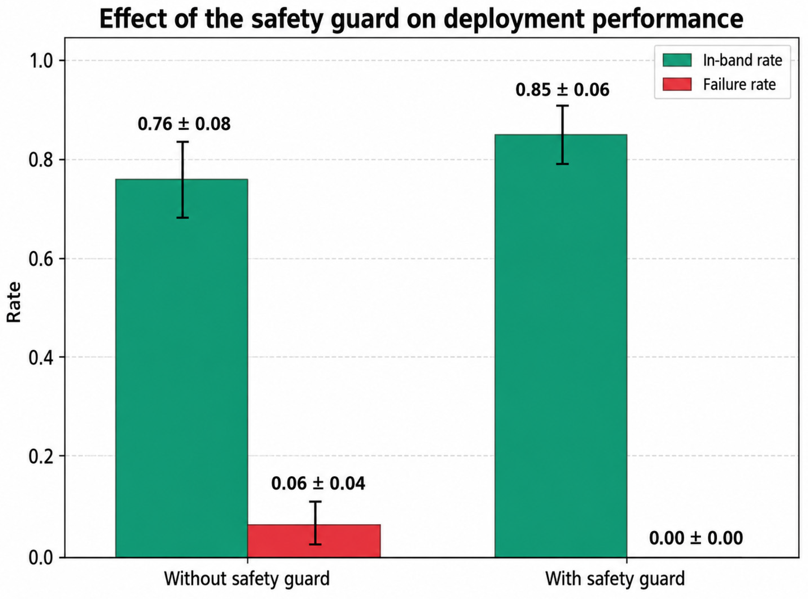
As shown in Table 11, deployment reliability is quantified as 1 − Failure Rate. Without the safety guard, the FM-BiGRU-DQN policy achieved an in-band rate of 0.76 ± 0.08 and a failure rate of 0.06 ± 0.04, corresponding to a deployment reliability of 0.94 ± 0.04. This indicates that the learned policy already provides relatively reliable maintenance decisions, but a small failure risk may still remain in high-risk degradation states, which reduces the practical reliability of the maintenance strategy.

After introducing the safety-guided execution mechanism, the failure rate decreased from 0.06 ± 0.04 to 0.00 ± 0.00, and the deployment reliability increased from 0.94 ± 0.04 to 1.00 ± 0.00. Meanwhile, the in-band rate increased from 0.76 ± 0.08 to 0.85 ± 0.06. These results show that the safety guard effectively eliminates the observed failures in this evaluation while improving the probability that maintenance is triggered within the desired target maintenance window.

It should be noted that the safety guard is not simply an engineering patch, but a deployment-oriented reliability layer for reinforcement-learning-based maintenance optimization. In normal degradation regions, the DQN policy preserves its adaptive decision-making ability. In high-risk regions, the safety guard enforces conservative intervention to avoid unsafe continuation decisions. Therefore, the combination of the learned policy and safety-guided execution improves both adaptability and reliability, which is particularly important for predictive maintenance applications where the cost of a wrong continuation decision is much higher than the cost of a conservative maintenance action.

4.11. Sensitivity Analysis of the Target Maintenance Window

The target maintenance window determines whether a maintenance action is regarded as a just-in-time intervention. In the main experiments, the window was set to [10, 50] steps before failure. To examine whether the proposed method depends strongly on this setting, three target maintenance windows were compared: [5, 30], [10, 50], and [20, 80].

For the $i$-th test trajectory, the lead time is defined as

$${\mathcal{l}}_i=t_{f,i}-t_{m,i},{\mathcal{l}}_i=t_{f,i}-t_{m,i}$$

(40)

where $t_{f,i}$ is the failure time and $t_{m,i}$ is the maintenance time.

For a target maintenance window $[{\tau }_{\min },{\tau }_{\max }]$, the in-band rate is calculated as

$$\mathrm{In}0\mathrm{band} \mathrm{Rate}={\displaystyle \frac{1}{N}}{\displaystyle \sum _{i=1}^N\mathbb{I}}\left({\tau }_{\min }\le {\mathcal{l}}_i\le {\tau }_{\max }\right)$$

(41)

where $N$ is the number of test trajectories and $\mathbb{I}(\cdot )$ is the indicator function.

The sensitivity results are summarized in

Table 12. Target window sensitivity.

Target Maintenance Window	Mean Lead Time	In-Band Rate	Failure Rate
[5, 30]	22.4	0.71	0.06
[10, 50]	31.7	0.85	0.00
[20, 80]	58.2	0.87	0.00

.

As shown in Table 12, the target maintenance window affects both maintenance timeliness and failure risk. When the window is set to [5, 30], the maintenance action is expected to occur closer to the failure point. This setting improves the utilization of useful life, but the safety margin becomes smaller. As a result, the failure rate increases to 0.06.

When the window is set to [10, 50], the proposed method achieves a mean lead time of 31.7, an in-band rate of 0.85, and a failure rate of 0.00. This result indicates that the window [10, 50] provides a suitable balance between avoiding delayed maintenance and preventing excessively early maintenance.

When the window is extended to [20, 80], the failure rate remains 0.00 and the in-band rate slightly increases to 0.87. However, the mean lead time increases to 58.2, indicating that the learned policy becomes more conservative and tends to trigger maintenance earlier. Although this setting improves safety, it may reduce the effective utilization of the remaining useful life.

Therefore, the target maintenance window [10, 50] was selected in the main experiments because it provides a practical just-in-time maintenance region. Compared with the later window [5, 30], it offers a larger safety margin. Compared with the earlier window [20, 80], it avoids overly conservative maintenance actions. These results show that the proposed FM-BiGRU-DQN method remains effective under different maintenance-window settings, while [10, 50] provides a balanced trade-off between reliability and maintenance efficiency.

4.12. Robustness Across Random Seeds

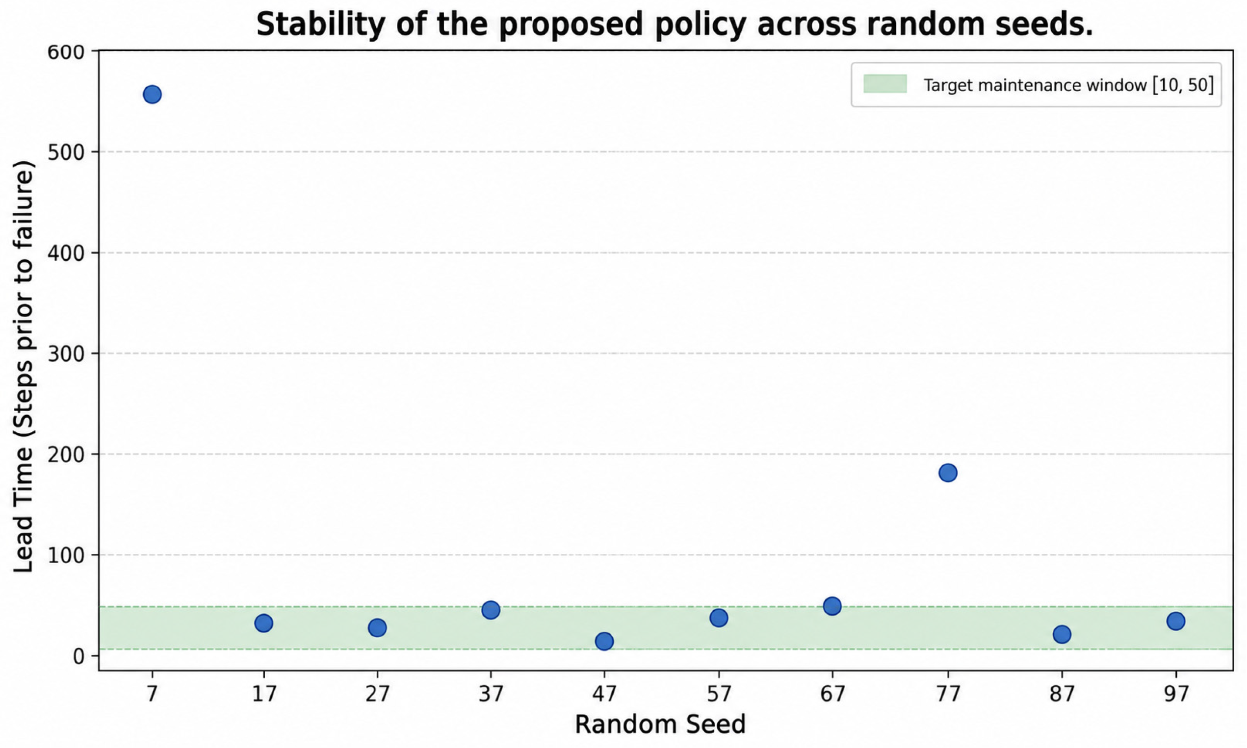
To further evaluate the robustness of the proposed method, repeated experiments were conducted under different random seeds. The resulting maintenance lead times are shown in Figure 9. Quantitatively, the repeated-seed evaluation shows that the proposed FM-BiGRU-DQN with safety-guided execution achieved a mean lead time of 33.9 ± 12.6 steps, an in-band rate of 0.85 ± 0.06, a failure rate of 0.00 ± 0.00, and a deployment reliability of 1.00 ± 0.00 across 10 independent random seeds. These numerical values indicate that the policy remains concentrated near the desired maintenance region while avoiding observed failure cases.

For most random seeds, FM-BiGRU-DQN produces maintenance decisions that fall within or close to the target maintenance window. This indicates that the proposed framework is generally stable across repeated training runs. The concentration of most lead times around the desired intervention region further confirms that the learned policy is not merely the result of a favorable random initialization.

At the same time, a few random seeds still produce larger lead times, indicating that the training process remains somewhat sensitive to stochastic initialization. This phenomenon is common in deep reinforcement learning, especially when the training data are limited and the degradation trajectories have strong nonlinear and nonstationary characteristics.

Nevertheless, the overall trend remains favorable. Most runs are concentrated around the target maintenance region, and extreme cases account for only a small proportion of the results. When considered together with the high in-band rate and zero failure rate achieved after safety-guided execution, these results support the robustness and practical reliability of the proposed FM-BiGRU-DQN framework.

4.13. Computational Efficiency and Deployment Feasibility

For industrial predictive maintenance applications, the computational cost of the decision model is an important practical consideration. Therefore, we further evaluated the training time, inference time, and computational complexity of the proposed FM-BiGRU-DQN framework.

All runtime measurements were conducted on a workstation equipped with AMD Ryzen 9 9950X3D CPU and NVIDIA GeForce RTX 5080 GPU. To reduce measurement bias, the inference time was averaged over repeated decision steps using the trained model under the evaluation mode. Data loading and visualization time were excluded from the reported inference latency.

The computational cost of the proposed framework mainly comes from three parts: fractional-memory state construction, BiGRU-based Q-value approximation, and DQN parameter updating. For each decision step, the fractional-memory state construction requires a fixed-length historical aggregation over the memory window, leading to a time complexity of $O\left(L{d}_x\right)$, where $L$ is the memory length and $d_x$ is the input feature dimension. Since $L=30$ in this study, this part introduces only a small constant overhead.

The BiGRU encoder dominates the inference cost. Let $W$ denote the observation window length, $h$ the number of hidden units in each direction, and $n_l$ the number of BiGRU layers. The forward-pass complexity of the BiGRU-based Q-network can be approximated as $O\left(n_l{W}_h(h+d_x)\right)$.

The constant factors associated with bidirectional computation and GRU gates are omitted for clarity. The final fully connected Q-value output layer has a much smaller cost, approximately $O(h|\mathcal{A}|)$, where $\left|\mathcal{A}\right|$ is the number of maintenance actions. In this study, $\left|\mathcal{A}\right|=2$. The safety-guided execution mechanism only checks two scalar thresholds and therefore has $O\left(1\right)$ complexity.

Table 13. Computational efficiency of the proposed FM-BiGRU-DQN framework.

Hardware platform	AMD Ryzen 9 9950X3D CPU, NVIDIA GeForce RTX 5080 GPU
Training configuration	500 episodes, batch size 64, replay buffer 10,000
Model size	Approximately 1.09 × 105 trainable parameters
Training time	8.7 min for 500 episodes
Inference time	0.41 ms per decision step
Inference complexity	$O\left(L{d}_x\right)+O\left(n_l{W}_h(h+d_x)\right)+O\left(1\right)$
Deployment mode	Offline training and online inference

summarizes the measured computational efficiency of the proposed framework.

As shown in Table 13, the complete offline training process requires 8.7 min for 500 episodes on the adopted workstation. During online deployment, the average inference latency is 0.41 ms per decision step, which is much shorter than the monitoring interval of the bearing degradation process. Therefore, the proposed framework is computationally feasible for industrial predictive maintenance applications.

4.14. Discussion

The experimental results provide several important observations.

First, the R/S analysis confirms that rolling bearing degradation trajectories exhibit pronounced long-memory characteristics. This supports the basic motivation of the proposed method: predictive maintenance should not rely only on a short-memory or purely Markovian state representation when the underlying degradation process is history-dependent.

Second, the comparison among MDP-DQN, Fractional-MDP, NM-BiGRU-DQN, and FM-BiGRU-DQN shows that fractional-memory representation and sequential learning contribute differently to maintenance decision-making. Fractional-memory representation improves the state description by embedding historical degradation effects, while BiGRU-based sequence learning captures nonlinear temporal dependencies within the observation window. Their combination produces the most accurate and stable maintenance policy.

Third, the sensitivity analysis demonstrates that the fractional order plays a key role in balancing recent degradation variation and long-term historical memory. This result indicates that the fractional component is not merely an auxiliary feature, but an important modeling mechanism that directly affects decision performance.

Finally, the safety-guided policy execution mechanism improves deployment reliability by preventing unsafe continuation decisions near the failure boundary. This makes the proposed framework more suitable for practical predictive maintenance scenarios, where safety and reliability are as important as decision optimality.

Overall, the results show that the proposed FM-BiGRU-DQN framework provides an effective hybrid modeling strategy for long-memory degradation systems. By integrating fractional-order memory representation, deep sequential representation learning, and reinforcement-learning-based policy optimization, the framework can improve maintenance timing precision, reduce failure risk, and enhance deployment robustness.

It should also be noted that the current framework uses only RMS as the health indicator. This setting provides a stable and reproducible degradation trajectory for evaluating the proposed fractional-memory reinforcement learning framework, but it may not fully capture subtle early-stage degradation patterns. For example, weak impulsive components, local defects, and non-stationary frequency-domain variations may be better reflected by indicators such as kurtosis, crest factor, spectral kurtosis, envelope-spectrum features, and time–frequency features. Therefore, the current RMS-based setting represents a simplified and controlled evaluation scenario. Incorporating multi-domain health indicators into the fractional-memory state representation is a promising direction for further improving the sensitivity and generalization ability of the proposed maintenance decision model.

5. Conclusions

This study proposed a hybrid fractional-memory deep reinforcement learning framework for predictive maintenance of long-memory degradation systems. Motivated by the non-Markovian and history-dependent nature of rolling bearing degradation, the predictive maintenance problem was reformulated as a fractional-state sequential decision problem. In the proposed FM-BiGRU-DQN framework, the Grünwald–Letnikov fractional difference operator was used to construct a memory-aware degradation state, the BiGRU network was employed to learn nonlinear sequential representations, and the DQN module was adopted to optimize maintenance actions under uncertain degradation evolution.

The experimental results on the IEEE PHM 2012 and XJTU-SY bearing degradation datasets demonstrate the effectiveness and cross-dataset robustness of the proposed framework. First, the combined R/S and DFA analyses indicate that the bearing degradation trajectories exhibit persistent long-memory characteristics, while the DFA results provide a more robust verification after detrending. Second, the comparison with MDP-DQN, Fractional-MDP, and NM-BiGRU-DQN shows that the proposed FM-BiGRU-DQN achieves a more desirable maintenance lead-time distribution, a higher in-band rate, and a lower failure risk. These results indicate that fractional-memory representation and BiGRU-based sequential learning are complementary: the former explicitly embeds nonlocal historical degradation information, while the latter captures nonlinear temporal evolution within the observation window. Third, the sensitivity analysis of the fractional order shows that an appropriate fractional order can effectively balance recent degradation variation and accumulated historical memory, thereby improving maintenance timing precision. Finally, the safety-guided execution mechanism further enhances deployment reliability by preventing unsafe continuation decisions near the failure boundary.

Overall, the results suggest that predictive maintenance for rolling bearing degradation should not be treated as a purely Markovian decision problem. By embedding fractional-memory degradation information into the reinforcement learning state, the proposed framework reduces the mismatch between long-memory degradation dynamics and standard Markovian policy learning. Therefore, FM-BiGRU-DQN provides a data-driven hybrid modeling strategy that integrates fractional-order degradation representation, deep sequential learning, and reinforcement-learning-based maintenance optimization for complex memory-dependent systems.

Several limitations remain for future investigation. First, the current framework uses RMS as the only health indicator. Although RMS provides a stable, reproducible, and physically interpretable degradation trajectory, it may not fully capture subtle early-stage degradation patterns, such as weak impulsive components, local defects, and non-stationary frequency-domain changes. Future work will incorporate multi-domain health indicators, including kurtosis, skewness, crest factor, peak-to-peak value, spectral kurtosis, envelope-spectrum features, and time–frequency features, to improve the sensitivity of the proposed framework to subtle degradation behavior. Second, the current framework uses a fixed-order Grünwald–Letnikov fractional operator, whereas real degradation processes may exhibit time-varying memory intensity under different operating conditions. Future work will investigate variable-order fractional modeling to adaptively characterize changing degradation memory. Third, the fractional component in this study is used as a discrete memory representation rather than as a fully physics-informed fractional differential equation model. Future research may further combine fractional differential equations, physics-informed neural networks, and reinforcement learning to improve the interpretability and generalization ability of predictive maintenance models. Finally, the proposed framework should be validated on more industrial datasets and under variable working conditions to further examine its robustness in practical deployment scenarios.