Fractional Memory-Driven Marine Predator Optimization for Nonconvex Economic Load Dispatch in Renewable-Integrated Power Systems

Abstract

The increasing integration of renewable energy sources (RESs) and the nonlinear nature of economic load dispatch (ELD) have significantly intensified the complexity of modern power systems, demanding efficient optimization techniques. This study proposes a Fractional Marine Predators Algorithm (FMPA) to address the ELD problem under uncertain and stochastic operating conditions. The proposed approach enhances the conventional MPA by incorporating fractional calculus (FC), which introduces memory-dependent search dynamics and improves the balance between exploration and exploitation. This modification enables the algorithm to utilize historical search information, resulting in smoother convergence behavior and reduced susceptibility to premature convergence. The performance of the proposed method is assessed using multiple benchmark systems, including 3-unit, 13-unit, and 40-unit configurations with integrated wind power. The optimization framework considers realistic system constraints such as generator limits, valve-point loading effects, and stochastic wind power modeled using probabilistic functions. Simulation results demonstrate that FMPA provides competitive and near-optimal generation costs with stable convergence behavior compared to several existing metaheuristic techniques. Statistical analysis over multiple independent runs confirms the robustness, stability, and reliability of the proposed method. The results indicate that FMPA provides a scalable and efficient solution for solving complex, nonlinear, and constrained ELD problems in modern power systems.

1. Introduction

1.1. Motivation and Inspiration

Electricity consumption has experienced sustained growth in recent decades, driven by rapid urban development, increasing population density, and the widespread adoption of electrical technologies across residential, commercial, and industrial sectors. Concurrently, the increasing integration of renewable energy sources (RESs), which are inherently intermittent and uncertain, has further complicated the operation of modern power systems. As a result, power networks are subjected to greater operational stress, leading to increased costs related to generation, operation, and maintenance, along with heightened risks of system losses, instability, and potential outages. Within this framework, the ELD problem has become a critical aspect of power system operation, particularly due to the rising cost of electricity generation and the progressive depletion of fossil fuel reserves used in conventional thermal units. The ELD problem aims to determine the optimal allocation of real power output among available generating units while adhering to system constraints. Its primary objective is to minimize total generation cost while ensuring reliable and efficient system performance. In this study, wind power uncertainty is incorporated into a stochastic steady-state ELD model, where variability is captured through expected penalty costs associated with overestimation and underestimation, rather than relying on real-time or time-coupled day-ahead dispatch strategies.

1.2. Literature Review

The continuous rise in electricity demand has led to a substantial increase in generation costs, highlighting the necessity for efficient and economical power dispatch strategies to reduce fuel consumption while maintaining reliable grid operation [1,2]. The ELD problem is fundamentally concerned with determining an optimal allocation of generation among available units such that the total demand is satisfied at minimum cost, while complying with all operational and system constraints. A wide range of traditional optimization algorithms have been suggested to solve this problem, such as Newton–Raphson algorithms, lambda iteration, dynamic programming, and gradient-based methods. Still, all these techniques suffer from certain disadvantages. Thus, for example, gradient-based methods usually take considerable time to work and experience some problems in solving inequality constraints [3]. The performance of the Newton–Raphson algorithm largely depends on the initial value, which can lead to unsatisfactory results in some cases. Linear programming relies on piecewise linear approximations, reducing accuracy, while quadratic programming can become inefficient with improper step size selection, especially for piecewise quadratic problems [3]. Moreover, interior-point methods, despite their efficiency, do not guarantee practical solutions for nonlinear problems [4].

Furthermore, the conventional methods generally assume the incremental cost curve to be smooth and monotonically increasing, which does not hold true for real-life power system scenarios. The ELD problem itself is non-convex, nonlinear, and non-smooth, among many other considerations [5]. To address these challenges and overcome the shortcomings of conventional approaches, numerous soft computing and metaheuristic methods have been introduced in recent years. Several advanced optimization approaches have been designed for solving the difficulties posed by the ELD problem. Application of ABC optimization is found in [6] to solve the ELD problems under valve-point loading effect for several IEEE test systems having three-, thirteen-, and forty-unit systems. Similarly, hybrid approaches such as BB–BC combined with PSO [7] and PSO integrated with pattern search [8] have demonstrated improved robustness and faster convergence. The ELD problem based on valve-point loading effect has been optimized using ant lion optimizer in [9], whereas gray wolf optimizer (GWO) is applied in [10]. Invasive weed optimization is used in [11] considering valve-point effect and prohibited zones.

Hybridization and adaptation of metaheuristics have been investigated in earlier works as well. In [12], a combination of bacterial foraging and PSO algorithms was used for tackling non-convex ELD with valve-point effects. Moreover, in [10], an adaptive PSO method that uses adaptive acceleration coefficients was developed to modify the search procedure and optimize the fitness function. Moreover, multi-objective approaches using PSO algorithm have been studied, in which PSO was used for solving multi-ELD in [13] considering generation cost and transmission loss at the same time. More recently, optimization approaches based on learning and intelligence are explored. An optimization approach for ELD problem, using Q-learning technique, was proposed in [14] that works efficiently for ELD problems in IEEE benchmark test systems. Moreover, a quasi-quadratic programming model with powerful exploitation capabilities was proposed in [15] for smart building systems’ ELD problem.

Chameleon swarm algorithm was used in [16] as a metaheuristic algorithm for ELD problem solution. On the other hand, pigeon-inspired oppositional optimization approach was presented in [17] to avoid premature convergence in power system ELD problem. Differential evolution (DE) method with tournage-best vector for the mutation process was proposed in [18] for efficient optimization of ELD problem. Improved teaching–learning-based optimization (TLBO) method using quasi-oppositional learning was proposed in [19] to improve exploration and convergence properties of TLBO method. An integrated comparative analysis was performed in [20] for solving the dynamic ELD problem using several soft computing techniques such as DE, PSO, evolutionary programming (EP), genetic algorithm (GA), and simulated annealing (SA). In [21], DE optimization technique was utilized to remove inefficient generating units, resulting in an impressive fuel cost savings of around 19.88% compared to traditional methods. In [22], a unique form of PSO optimization algorithm, known as the catfish PSO, was devised to handle the problem of ELD under valve-point loading effect efficiently. Furthermore, a novel hybrid optimization algorithm combining GA and DE with a dynamic pattern search (PS) search method was suggested in [23] for solving ELD problem with valve-point effects.

The production of electricity using fossil fuel-based thermal power plants has been largely responsible for the emission of pollutants such as NOx, SOx, and CO. Computational and optimization approaches have thus been introduced to improve efficiency in generation and reduce pollution as well. An exchange market algorithm (EMA) was adopted in [24] to optimize the ELD problem in cases where wind power exists. A similar approach involving a hybrid optimization method known as HIC-SQP was proposed in [25] for optimal coordination between wind power and thermal generation to minimize cost and pollutant emissions. PSO, a widely used metaheuristic algorithm based on collective intelligence, was also employed in [26,27] to find the optimum solution for ELD with wind power generation in hybrid power systems. The rise in RESs, mainly solar and wind, has played an important role in alleviating the economic as well as environmental issues related to traditional power generation [28,29,30,31]. However, due to the uncertainty associated with renewable sources, conventional fuel cost functions require modification. For example, probabilistic models such as Beta and Weibull distributions have been incorporated to capture the variability of solar and wind power generation, respectively [18].

Recent studies have proposed the integration of FC, especially fractional derivatives that are not integers, within the mathematical representation of the systems for better modeling and optimization purposes [32,33]. This method has proven effective when used to solve different kinds of problems such as feature selection, fractional-order filters, Kalman filters, and even robotic manipulator control. It has become common practice to integrate fractional calculus with the metaheuristic technique of optimization to solve optimization problems in power systems. Numerous investigations have focused on exploring fractional-order versions of classic optimization algorithms. For instance, the fractional-order PSO algorithm has been used to optimize different types of engineering problems [34,35,36,37,38], while a combination of dynamic methods based on genetic algorithms and particle swarm optimization has been employed for designing multi-band power system stabilizers [39] and nonlinear system identification [40]. Furthermore, fractional-order modifications of the moth-flame optimization algorithm have proved to be efficient tools for addressing complicated engineering optimization problems [41,42]. Altogether, all these investigations demonstrate that the incorporation of FC into metaheuristic algorithms is a powerful approach for dealing with complex optimization problems in contemporary power and energy systems.

1.3. Contribution and Paper Structure

Metaheuristic optimization methods often require careful parameter tuning, and obtaining high-quality solutions may involve considerable computational effort. To address these challenges, this study introduces a Fractional Marine Predators Algorithm (FMPA) for solving nonconvex ELD problems. The proposed method is inspired by the natural foraging behavior of marine predators and preserves the original MPA search mechanism based on Brownian motion, Lévy flight, predator–prey interactions, and phase-dependent exploration–exploitation behavior.

Although fractional calculus has been incorporated into several swarm intelligence algorithms, such as PSO [36], GWO [28], WOA [5], and MFO [41,42], its integration with the Marine Predators Algorithm for renewable-integrated ELD problems remains comparatively less explored. Therefore, the novelty of this work is not that it claims to propose a new fractional calculus theory, but rather a methodological enhancement of MPA through the incorporation of a Grünwald–Letnikov fractional memory mechanism. Unlike conventional fractional variants that mainly modify direct position or velocity updates, the proposed FMPA embeds fractional memory into the velocity-like movement dynamics of MPA while retaining its Brownian–Lévy phase-based search structure.

The fractional memory mechanism enables each search agent to utilize information from previous movement states during the optimization process. This memory-driven behavior helps smooth abrupt search variations, improves convergence stability, and supports a better balance between exploration and exploitation. As a result, the proposed FMPA provides a competitive and scalable optimization framework for solving nonlinear, nonconvex, and stochastic ELD problems under renewable energy uncertainty.

The main contributions of this study are summarized as follows:

• FMPA is developed by incorporating a Grünwald–Letnikov fractional memory mechanism into the standard MPA framework, introducing memory-driven search dynamics while preserving the original Brownian–Lévy predator–prey structure.
• A comprehensive ELD formulation is established, considering generator operating limits, and stochastic wind power is modeled using the incomplete gamma function.
• The performance of the proposed FMPA is evaluated on multiple benchmark systems, including 3-unit, 13-unit, and 40-unit test cases, demonstrating its effectiveness across different system scales.
• Comparative analyses with existing state-of-the-art metaheuristic techniques show that FMPA achieves improved solution quality and faster convergence behavior.
• Statistical results confirm the robustness and reliability of the proposed method, indicating consistent performance and stable convergence under uncertain operating conditions.

The rest of this paper is organized as follows: Section 2 describe the formulation of the ELD problem under the consideration of valve-point loading effect (VPLE) and uncertainty of wind power generation modeled by using the incomplete gamma function (IGF). In Section 3, the new FMPA approach is discussed, which includes the procedure of the approach as well as the pseudocode. Simulation results with the comparison of performance for various test scenarios (i.e., case 1, case 2, and case 3) are provided in Section 4.

2. Mathematical Modelling of ELD

The primary objective of the ELD problem is to determine the optimal power output of generating units while minimizing the total generation cost and satisfying system operating constraints. For thermal units without valve-point loading effects, the conventional quadratic fuel cost function is expressed as [43,44].

$${C_T}^{quad}={\displaystyle \sum _{i=1}^N} \left(a_i+b_i{P}_i+c_i{P}_i^2\right)$$

(1)

where $P_i$ is the power output of the ith thermal generating unit, and $a_i$, $b_i{, c}_i$, are the corresponding fuel cost coefficients.

When valve-point loading effects are considered, the fuel cost curve becomes non-smooth due to the rippling effect caused by the valve-opening process. In this case, the thermal generation cost is expressed as

$${C_T}^{VPLE}={\displaystyle \sum _{i=1}^N} \left(a_i+b_i{P}_i+c_i{P}_i^2+\left|d_i\sin \left(e_i\left(P_i^{\mathrm{m}\mathrm{i}\mathrm{n}}-P_i\right)\right)\right|\right)$$

(2)

where $d_i$ and $e_i$ are the valve-point loading coefficients of the ith generating unit, and $P_i^{\mathrm{m}\mathrm{i}\mathrm{n}}$ is the minimum generation limit. It is important to note that ${C_T}^{VPLE}$ already contains the quadratic thermal cost component. Therefore, the valve-point cost function substitutes the conventional quadratic cost function when valve-point loading effects are considered; both terms are not added together.

The integration of wind power improves economic and environmental performance; however, the stochastic nature of wind speed introduces uncertainty in available wind generation. The total wind-related cost is formulated as

$$C_{\mathrm{wind} }={\displaystyle \sum _{k=1}^{Nw}} \left[C_k^{\mathrm{d}\mathrm{i}\mathrm{r}}+C_k^{\mathrm{o}\mathrm{v}\mathrm{e}\mathrm{r}}+C_k^{\mathrm{u}\mathrm{n}\mathrm{d}\mathrm{e}\mathrm{r}}\right]$$

(3)

where $C_k^{\mathrm{d}\mathrm{i}\mathrm{r}}, C_k^{\mathrm{o}\mathrm{v}\mathrm{e}\mathrm{r}}$, and $C_k^{\mathrm{u}\mathrm{n}\mathrm{d}\mathrm{e}\mathrm{r}}$ denote the direct wind generation cost, overestimation penalty cost, and underestimation penalty cost of the kth wind unit, respectively.

The direct wind power cost is expressed by

$$C^{\mathrm{d}\mathrm{i}\mathrm{r}}={\displaystyle \sum _{k=1}^{Nw}} \left({\alpha }_k{W}_k\right)$$

(4)

where ${\alpha }_k$ is the direct cost coefficient and $W_k$ is the scheduled wind power of the kth wind unit.

The overestimation cost occurs when the scheduled wind power is higher than the actual available wind power. In this case, reserve power is required to compensate for the deficit. It is expressed as

$$C^{\mathrm{o}\mathrm{v}\mathrm{e}\mathrm{r}}={\displaystyle \sum _{k=1}^{Nw}} {\rho }_{k}E\left[{(W_{s,k}-W_{a,k})}^{+}\right]$$

(5)

where $W_{s,k}$ and $W_{a,k}$ denote the scheduled and available wind power of the kth wind unit, respectively; ${\rho }_k$ is the overestimation penalty coefficient; and ${\left(Z\right)}^{+}=max(z,0)$

The underestimation cost occurs when the available wind power exceeds the scheduled wind power, resulting in surplus energy that may require compensation. It is expressed as

$$C^{under}={\displaystyle \sum _{k=1}^{Nw}} {\delta }_{k}E\left[{(W_{a,k}-W_{s,k})}^{+}\right]$$

(6)

where ${\delta }_k$ is the underestimation penalty coefficient. Thus, the overestimation cost represents the expected deficit penalty, whereas the underestimation cost represents the expected surplus compensation.

The wind power uncertainty is modeled using the Weibull distribution and incomplete gamma function. The incomplete gamma function is defined as

$$\mathsf{\Gamma }\left(a,b\right)={\displaystyle \frac{1}{\mathsf{\Gamma }\left(a\right)}}{\int }_0^b t^{a-1}{e}^{-t}dt$$

(7)

where $\mathsf{\Gamma }\left(a\right)$ is the standard gamma function.

2.1. Total Generation Cost

Based on the operating condition of the test system, the total objective function is defined as

$$C_{\mathrm{total} }=\left\{\begin{array}{c}{C_T}^{quad}, for thermal system without VPLE\\ {C_T}^{VPLE}, for thermal system with VPLE\\ {C_T}^{VPLE}+C_{\mathrm{wind} } , for wind integreated system with VPLE\end{array}\right.$$

(8)

2.2. Power Constraints

The key constraint in the management of power systems is to make sure that the total generation of power meets the load requirements for optimum performance.

$${\displaystyle \sum _{i=1}^N} G_i=D+L$$

(9)

The power balance condition is represented by the following relation: the sum of the generated powers Gi for all the N generation units equals the sum of load demand D and transmission losses L. It makes sure that enough power has been generated to meet the required demand.

2.3. Generator Operating Limits

In the ELD formulation, each generating unit must operate within its prescribed minimum and maximum output limits. This constraint can be expressed as:

$$G_{Ni}^{\mathrm{m}\mathrm{i}\mathrm{n}}\le G_{Ni}\le G_{Ni}^{\mathrm{m}\mathrm{a}\mathrm{x}},\mathrm{i}=\mathrm{1,2},\dots ,N$$

(10)

where $G_{Ni}^{\mathrm{m}\mathrm{i}\mathrm{n}}$ and $G_{Ni}^{\mathrm{m}\mathrm{a}\mathrm{x}}$ are the minimum and maximum power outputs (MW) that can be delivered by the Nth generator, respectively. The above inequality guarantees that every generator runs within its capacity constraints.

3. Design Methodology Using FMPA

3.1. Marine Predators Algorithm

The MPA is a nature-inspired technique that mimics the hunting behavior of marine creatures, and the dynamics involved between the predator and its prey [45]. Brownian and Lévy movements are used by MPA to improve the search process and optimize exploration. This section outlines these motion mechanisms and explains their integration into the MPA framework.

3.1.1. Brownian Motion

Brownian motion is a stochastic process whose movements are random and continuous with their step sizes being normally distributed with a zero mean (μ = 0) and a variance (σ² = 1). This implies Brownian motion is unbiased, with the probability of move being equal from all directions. Also, the size of each step is very small and localized. It is this characteristic that makes the Brownian motion ideal for modelling local search or exploitation within optimization models. It is the stochastic nature of the process that will allow for steady exploration and exploitation within the search space. The probability density function (PDF) of the Brownian motion, which provides the probability of making a step to point x, is expressed by [46].

$$f_B\left(x;\mu ,\sigma \right)={\displaystyle \frac{1}{\sqrt{2\pi {\sigma }^2}}}\mathrm{e}\mathrm{x}\mathrm{p}\left(-{\displaystyle \frac{{\left(x-\mu \right)}^2}{2{\sigma }^2}}\right)={\displaystyle \frac{1}{\sqrt{2\pi }}}\mathrm{e}\mathrm{x}\mathrm{p}\left(-{\displaystyle \frac{x^2}{2}}\right)$$

(11)

3.1.2. Lévy Motion

Lévy motion, also referred as Lévy flight, is a class of stochastic random walk characterized by occasional long jumps combined with many short steps. Unlike Brownian motion, which follows a normal distribution, Lévy motion exhibits a heavy tailed probability distribution, thereby facilitating the exploration of faraway areas in the solution space. This trait renders Lévy flight a suitable strategy in the improvement of global exploration in optimization techniques. The numbers drawn from the Lévy probability distribution function can be stated as [47]

$$Levy\left(\alpha \right)=0.05\times {\displaystyle \frac{x}{{\left|y\right|}^{1/\alpha }}}$$

(12)

Lévy(α) denotes a random variable generated from the Lévy distribution, where the stability index α typically lies in the range 0.3 ≤ α ≤ 1.99. The variables x and y are independent random numbers drawn from normal distributions with standard deviations σ_x and σ_y, respectively, which are defined as follows

$$x=Normal\left(0,{\alpha }_x^2\right)$$

(13)

$$y=Normal\left(0,{\alpha }_y^2\right)$$

(14)

The parameter σ_x can be calculated using the following expression:

$${\sigma }_x={\left[{\displaystyle \frac{\Gamma \left(1+\alpha \right)\mathrm{s}\mathrm{i}\mathrm{n}\left(\frac{\pi \alpha }{2}\right)}{\Gamma \left(\frac{\left(1+\alpha \right)}{2}\right)\alpha \cdot 2^{\frac{\left(\alpha -1\right)}{2}}}}\right]}^{{\displaystyle \frac{1}{\alpha }}} , \mathrm{Where} {\sigma }_y=1\mathrm{and} \alpha =1.5$$

(15)

where Γ represents the Gamma function. For positive integer values of x, it satisfies Γ(x) = (x − 1)!

3.1.3. Mathematical Formulation of the Marine Predators Algorithm

The MPA employs both Brownian and Lévy motion strategies to effectively balance the exploration and exploitation phases, thereby enhancing the likelihood of obtaining an optimal or near-optimal solution. Initially, the population of candidate solutions is generated using a uniform random distribution within the boundaries defined by the corresponding equation.

$$X_0=X_{\mathrm{m}\mathrm{i}\mathrm{n}}+rand\left(X_{\mathrm{m}\mathrm{a}\mathrm{x}}-X_{\mathrm{m}\mathrm{i}\mathrm{n}}\right)$$

(16)

where $X_0$ denote the initial position vector of the candidate solutions, while $X_{\mathrm{m}\mathrm{i}\mathrm{n}}$ and $X_{\mathrm{m}\mathrm{a}\mathrm{x}}$ represent the lower and upper bounds of the decision variables, respectively. The term rand refers to a random set of numbers that are generated from a uniform distribution ranging from zero to one. The next step involves computing the objective function on each of the candidate solutions in the population. After this step, the solution with the highest value in terms of the objective function is selected as the top predator. Based on the law of natural selection, the best candidate is used in constructing an elite matrix referred to as “Elite,” and this can be written as:

$$Elite={\left[\begin{array}{cccc}{X}_{\mathrm{1,1}}^T& X_{\mathrm{1,2}}^T& \dots & X_{1,d}^T\\ X_{\mathrm{2,1}}^T& X_{\mathrm{2,2}}^T& \dots & X_{2,d}^T\\ ⋮& ⋮& ⋮& ⋮\\ ⋮& ⋮& ⋮& ⋮\\ ⋮& ⋮& ⋮& ⋮\\ X_{n,1}^T& X_{n,2}^T& \dots & X_{n,d}^T\end{array}\right]}_{n\times d}$$

(17)

In this formulation, $X^T$ refers to the top predator vector that is duplicated n times to obtain the Elite matrix. In this case, n is the search population size and d is the dimension of the decision vectors. In the optimization process, predators and prey are considered as search population members. In nature, predators chase prey whereas prey chase resources. At the appearance of a more performing predator, the top predator will be updated, and hence, the Elite matrix will change in every cycle. Within each iteration, the location of predators is calculated using the Prey matrix whose dimension is like that of Elite matrix. To start with, the Prey matrix is constructed, and the best performing member is chosen to serve as the top predator that will be utilized for the construction of Elite matrix. The Prey matrix can be defined mathematically as follows:

$$Prey={\left[\begin{array}{cccc}{X}_{\mathrm{1,1}}& X_{\mathrm{1,2}}& \dots & X_{1,d}\\ X_{\mathrm{2,1}}& X_{\mathrm{2,2}}& \dots & X_{2,d}\\ ⋮& ⋮& ⋮& ⋮\\ ⋮& ⋮& ⋮& ⋮\\ ⋮& ⋮& ⋮& ⋮\\ X_{n,1}& X_{n,2}& \dots & X_{n,d}\end{array}\right]}_{n\times d}$$

(18)

where X denotes the position of each prey within the search space, with each element corresponding to a specific dimension of the problem.

Search Phases of the MPA

Within the optimization process, the MPA was divided into three phases based on the predator–prey velocity relationship that simulates various levels of predator–prey relationships at different points of time. A designated range of iterations is assigned to each phase, during which the movement patterns of both predators and prey are governed by mathematical formulations, as outlined below.

Phase A. In the initial phase, commonly referred to as the exploration stage, the predator exhibits a higher velocity compared to the prey, resulting in a large predator–prey speed ratio during the early iterations. In this phase, the prey actively explores the search space using a Brownian motion strategy to identify promising regions that may contain feasible solutions. Accordingly, the position of the prey is updated based on the following mathematical expressions, if the current iteration number is less than one-third of the maximum number of iterations.

$$\begin{array}{c}stepsiz{e}_i={\overrightarrow{R}}_B\otimes \left(Elit{e}_i-{\overrightarrow{R}}_B\otimes Pre{y}_i\right) ,i=1,\dots ,n\\ Pre{y}_i=Pre{y}_i+P\cdot \overrightarrow{R}\otimes stepsiz{e}_i\end{array}$$

(19)

In this expression, ${\overrightarrow{R}}_B$ denotes a vector of random values generated from a normal distribution to represent Brownian motion, while $\otimes$ indicates element-wise multiplication. The parameter P is a constant assigned a value of 0.5, and $\overrightarrow{R}$ represents a vector of random numbers uniformly distributed over the interval [0,1].

Phase B. This phase takes place during the intermediate stage of the optimization process, where the predator and prey exhibit comparable movement speeds, corresponding to a unit velocity ratio. At this stage, the algorithm transitions from exploration to exploitation. Accordingly, the population is divided into two equal groups: one subset (prey) is dedicated to exploration, while the other subset (predators) focuses on exploitation of the search space. From a mathematical point of view, the prey makes use of movements characterized by Lévy flight to improve its explorative behavior, while the predator adopts Brownian motion for enhancing exploitation behavior as depicted below, if the current iteration belongs to the intermediate range, i.e.,

$$\left({\displaystyle \frac{1}{3}}\right)\times maximum\_iteration<Iteration<\left({\displaystyle \frac{2}{3}}\right)\times maximum\_iteration$$

For the first half of the population, corresponding to the prey group, the position update is governed by the following expression:

$$\begin{array}{c}stepsiz{e}_i={\overrightarrow{R}}_L\otimes \left(Elit{e}_i-{\overrightarrow{R}}_L\otimes Pre{y}_i\right) ,i=1,\dots ,{\displaystyle \frac{n}{2}}\\ Pre{y}_i=Pre{y}_i+P\cdot \overrightarrow{R}\otimes stepsiz{e}_i\end{array}$$

(20)

In Equation (31), ${\overrightarrow{R}}_L$ denotes a vector of random values generated according to a Lévy distribution. The motion of the prey is modeled through the element-wise multiplication of ${\overrightarrow{R}}_L$ with the Prey matrix. Consequently, the resulting step size incorporated into the prey’s position reflects Lévy flight behavior, thereby enhancing the exploitation capability of the algorithm.

The remaining half of the population corresponds to the predator group.

$$\begin{array}{c}stepsiz{e}_i={\overrightarrow{R}}_B\otimes \left({\overrightarrow{R}}_B\otimes Elit{e}_i-Pre{y}_i\right) ,i=\left({\displaystyle \frac{n}{2}}\right)+1,\dots ,n\\ Pre{y}_i=Elit{e}_i+P\cdot CF\otimes stepsiz{e}_i\end{array}$$

(21)

In this formulation, the movement of the predator is modeled through the element-wise multiplication of ${\overrightarrow{R}}_B$ with the Elite matrix, representing Brownian motion behavior. The prey position is subsequently updated by incorporating the predator’s Brownian-based movement. The parameter $CF$ serves as an adaptive control factor that regulates the step size, and it can be determined as follows:

$$CF={\left(1-{\displaystyle \frac{Iter}{Ma{x}_{iter}}}\right)}^{\left(2{\displaystyle \frac{Iter}{Ma{x}_{iter}}}\right)}$$

(22)

where Iter denotes the current iteration number, while Max_iter represents the maximum number of iterations.

Phase C. The final step happens when the predator is faster than the prey in relation to a lower velocity ratio. The situation often emerges during the latter stages of the optimization process when exploitation is predominant. In this case, Lévy flight was deemed to be the optimal approach in simulating the movement of the predator at a lower velocity ratio (v = 0.1). It is represented mathematically as follows: if the current iteration exceeds two-thirds of the maximum number of iterations ($Iteration > \left({\displaystyle \frac{2}{3}}\right)\backslash times maximu{m}_{\left\{iteration\right\}}$), the algorithm enters the final phase.

$$\begin{array}{c}stepsiz{e}_i={\overrightarrow{R}}_L\otimes \left({\overrightarrow{R}}_L\otimes Elit{e}_i-Pre{y}_i\right) ,i=1,\dots ,n\\ Pre{y}_i=Elit{e}_i+P\cdot CF\otimes stepsiz{e}_i\end{array}$$

(23)

The predator’s movement is modeled using Lévy flight through the element-wise multiplication of ${\overrightarrow{R}}_L$ with the Elite matrix. The resulting step size is then incorporated into the Elite position to simulate predator dynamics, which in turn guides the update of the prey position, as expressed in Equation (32).

Impact of Eddy Formation and Fish Aggregating Devices (FADs)

Environmental conditions, including eddy formation and the presence of Fish Aggregating Devices (FADs), significantly influence the behavior of marine predators. According to [48], sharks spend over 80% of their time near FADs, while the remaining 20% is devoted to making long-range movements across different dimensions, likely to locate new prey distributions. In optimization terms, FADs can be associated with local optima where solutions may become trapped. The occasional long-distance movements help the algorithm escape these regions and continue exploring the search space. Therefore, the effect of FADs can be mathematically represented as follows:

$${ \mathrm{Prey}}_i=\left\{\begin{array}{c}{ \mathrm{Prey}}_i+CF\left[{\overrightarrow{X}}_{\mathrm{m}\mathrm{l}\mathrm{n}}+\overrightarrow{R}\otimes \left({\overrightarrow{X}}_{\mathrm{m}\mathrm{a}\mathrm{x}}-{\overrightarrow{X}}_{\mathrm{m}\mathrm{l}\mathrm{n}}\right)\right]\otimes \overrightarrow{U} \mathrm{i}\mathrm{f} r\le FADs\\ {\mathrm{P}\mathrm{r}\mathrm{e}\mathrm{y}}_i+\left[\mathrm{FADs} \left(1-r\right)+r\right]\left({\mathrm{Prey}}_{r1}-{\mathrm{Prey}}_{r2}\right) \mathrm{i}\mathrm{f} r>FADs\end{array}\right.$$

(24)

In this formulation, $\mathrm{FADs}$ = 0.2 denotes the influence of Fish Aggregating Devices on the optimization process. The vector U is a binary vector whose elements take values of either 0 or 1, generated randomly based on numbers uniformly distributed within the interval [0,1]. Each element is assigned a value of 0 when it is less than $\mathrm{FADs}$ and 1 when it exceeds $\mathrm{FADs}$. The parameter r represents a random number uniformly generated between 0 and 1. In addition, ${\overrightarrow{X}}_{\mathrm{m}\mathrm{l}\mathrm{n}}$ and ${\overrightarrow{X}}_{\mathrm{m}\mathrm{a}\mathrm{x}}$ indicate the lower and upper bounds of the search space, respectively, while $r1$ and $r2$ correspond to randomly selected indices from the Prey matrix.

Memory Retention Strategy in the MPA

A key feature of the MPA is the ability of marine predators to retain memory of locations where successful foraging has previously occurred, which is modeled through the marine memory saving mechanism. After updating the Prey matrix and incorporating the effects of FADs, the solutions are evaluated based on their fitness values to refine the Elite matrix. During each iteration, every current solution is compared with its corresponding solution from the previous iteration, and the better-performing one is retained. This iterative selection process progressively enhances solution quality and reflects the natural behavior of predators returning to regions with abundant prey following successful foraging experiences.

3.2. Fractional Marine Predators Algorithm (FMPA)

The proposed FMPA extends the standard MPA by incorporating fractional-order memory into its movement dynamics. In the conventional MPA, the search process is guided by Brownian and Lévy motions through different predator–prey interaction phases, enabling a balance between exploration and exploitation. However, the standard formulation relies mainly on the current search state. By integrating FC, the movement of each search agent becomes dependent not only on its current step but also on its historical trajectory, thereby introducing a long-memory effect that improves convergence smoothness, strengthens local exploitation, and reduces premature convergence.

FC is incorporated using the Grünwald–Letnikov (GL) definition, which is well suited for discrete-time numerical implementation. For a time-dependent function s(t), the GL fractional derivative of order δ is defined as [49,50]

$$D_{GL}^{\delta }[s(t)]=\underset{\Delta t\to 0}{\mathrm{l}\mathrm{i}\mathrm{m}} {\displaystyle \frac{1}{(\Delta t{)}^{\delta }}}{\displaystyle \sum _{j=0}^{\mathrm{\infty }}} (-1{)}^j{\displaystyle \frac{\mathsf{\Gamma }\left(\delta +1\right)}{\mathsf{\Gamma }\left(j+1\right)\mathsf{\Gamma }\left(\delta -j+1\right)}}s(t-j\Delta t),0<\delta <1$$

(25)

where Γ (⋅) denotes the Gamma function. For practical numerical implementation, the discrete approximation of the GL operator can be written as

$$D^{\delta }s(t)\approx {\displaystyle \frac{1}{T^{\delta }}}{\displaystyle \sum _{k=0}^N} (-1{)}^k\left({\displaystyle \genfrac{}{}{0pt}{}{\delta }{k}}\right)s(t-kT)$$

(26)

where T > 0 is the step size, N is the truncation length, and the generalized binomial coefficient is expressed as

$$\left({\displaystyle \genfrac{}{}{0pt}{}{\delta }{k}}\right)={\displaystyle \frac{\mathsf{\Gamma }\left(\delta +1\right)}{\mathsf{\Gamma }\left(k+1\right)\mathsf{\Gamma }\left(\delta -k+1\right)}}$$

(27)

In the standard MPA, the prey position is updated using a stochastic step generated from Brownian or Lévy motion according to the corresponding search phase. Since the MPA movement mechanism includes both the current position and a motion step, the fractional operator is more appropriately applied to the movement term rather than directly to the position. Let $P_i^t\in {\mathbb{R}}^d$ denote the position of the ith prey at iteration t and let ${S^t}_i$ denote the standard MPA step computed from the original phase-based update equations. A velocity-like memory state ${\mathrm{V}}_i^t$ is then introduced, and the prey position is updated as

$${\mathrm{P}}_i^{t+1}={\mathrm{P}}_i^t+{\mathrm{V}}_i^t$$

(28)

To incorporate fractional memory, the movement state is defined through a fractional-order relation as follows:

$$D^{\delta }{\mathrm{V}}_i^t=\alpha {\mathrm{S}}_i^t,\delta <1$$

(29)

where α is a scaling coefficient that controls the influence of the current MPA step. Applying the discrete GL approximation yields

$${\displaystyle \frac{1}{T^{\delta }}}{\displaystyle \sum _{k=0}^N} (-1{)}^k\left({\displaystyle \genfrac{}{}{0pt}{}{\delta }{k}}\right){\mathrm{V}}_i^{t-k}=\alpha {\mathrm{S}}_i^t$$

(30)

Assuming T = 1 for the iterative update, Equation (32) can be rearranged as

$${\mathrm{V}}_i^t=\alpha {\mathrm{S}}_i^t-{\displaystyle \sum _{k=1}^N} (-1{)}^k\left({\displaystyle \genfrac{}{}{0pt}{}{\delta }{k}}\right){\mathrm{V}}_i^{t-k}$$

(31)

For computational efficiency, the fractional expansion is truncated to a finite number of previous steps. By restricting the expansion to four memory terms, the fractional movement update becomes

$${\mathrm{V}}_i^t=\alpha {\mathrm{S}}_i^t+\delta {\mathrm{V}}_i^{t-1}+{\displaystyle \frac{\delta \left(1-\delta \right)}{2}}{\mathrm{V}}_i^{t-2}+{\displaystyle \frac{\delta \left(1-\delta \right)\left(2-\delta \right)}{6}}{\mathrm{V}}_i^{t-3}+{\displaystyle \frac{\delta \left(1-\delta \right)\left(2-\delta \right)\left(3-\delta \right)}{24}}{\mathrm{V}}_i^{t-4}$$

(32)

Substituting Equation (32) into the prey position update results in the final FMPA formulation:

$${\mathrm{P}}_i^{t+1}={\mathrm{P}}_i^t+\alpha {\mathrm{S}}_i^t+\delta {\mathrm{V}}_i^{t-1}+{\displaystyle \frac{\delta \left(1-\delta \right)}{2}}{\mathrm{V}}_i^{t-2}+{\displaystyle \frac{\delta \left(1-\delta \right)\left(2-\delta \right)}{6}}{\mathrm{V}}_i^{t-3}+{\displaystyle \frac{\delta \left(1-\delta \right)\left(2-\delta \right)\left(3-\delta \right)}{24}}{\mathrm{V}}_i^{t-4}.$$

(33)

In this formulation, ${\mathrm{S}}_i^t$ is obtained from the original MPA search mechanism, including the Brownian-based exploration phase, the mixed Brownian–Lévy transition phase, and the Lévy-dominant exploitation phase. Therefore, the proposed FMPA preserves the intrinsic predator–prey search behavior of MPA while enriching it with a fractional-order memory effect. The parameter δ ∈ (0, 1) acts as a fractional memory-shaping parameter that controls the weighting pattern assigned to previous movement states. In the truncated four-term expansion, the historical velocity components are weighted by ${\displaystyle \frac{\delta \left(1-\delta \right)}{2}}, {\displaystyle \frac{\delta \left(1-\delta \right)\left(2-\delta \right)}{6}} \mathrm{a}\mathrm{n}\mathrm{d} {\displaystyle \frac{\delta \left(1-\delta \right)\left(2-\delta \right)\left(3-\delta \right)}{24}}$. Therefore, δ should not be interpreted as a simple monotonic measure of memory strength. Instead, it regulates how the memory contribution is distributed among recent and older movement states. When δ approaches unity, the most recent velocity term becomes dominant, while higher-order historical terms become relatively small. For intermediate fractional values, the memory effect is distributed more gradually across previous movement states, which helps smooth abrupt changes in search trajectories and improves convergence stability. Thus, the fractional memory mechanism enables FMPA to retain useful historical search information while preserving the original Brownian–Lévy movement structure of MPA. The four-term memory truncation is adopted to balance historical information retention and computational efficiency. A shorter memory length may not sufficiently capture previous movement behavior, whereas a longer expansion increases computational burden with limited additional benefit. Therefore, the four-term approximation is used as a practical compromise that preserves recent movement history while keeping the algorithm computationally efficient. The pseudocode of the proposed FMPA is shown in Algorithm 1.

Algorithm 1. Pseudocode of FMPA
Step	Description
1	Initialize prey population ${ \mathrm{Prey} }_i(i=\mathrm{1,2},\dots ,n)$ within ($X_{\mathrm{m}\mathrm{i}\mathrm{n}},X_{\mathrm{m}\mathrm{a}\mathrm{x}}$)
2	Initialize fractional velocity states ($V_i$= 0)
3	Evaluate fitness of all prey and determine ($X_{best}$)
4	Construct Elite matrix using ($X_{best}$)
5	For $iter=1$ to ($Max-iter$)
6	Compute step vector $S_i$ based on MPA phases:
7	• Phase A: Brownian motion if $(Iter<{\displaystyle \frac{1}{3}}Max-iter)$
8	• Phase B: Brownian/Lévy if (${\displaystyle \frac{1}{3}}Max-iter\le {\displaystyle \frac{2}{3}}Max-iter)$
9	• Phase C: Lévy motion if ($Iter<{\displaystyle \frac{2}{3}}Max-iter)$
10	Update fractional velocity:
11	${\mathrm{V}}_i^t=\alpha {\mathrm{S}}_i^t+\delta {\mathrm{V}}_i^{t-1}+{\displaystyle \frac{\delta \left(1-\delta \right)}{2}}{\mathrm{V}}_i^{t-2}+{\displaystyle \frac{\delta \left(1-\delta \right)\left(2-\delta \right)}{6}}{\mathrm{V}}_i^{t-3}+{\displaystyle \frac{\delta \left(1-\delta \right)\left(2-\delta \right)\left(3-\delta \right)}{24}}{\mathrm{V}}_i^{t-4}$
12	Update prey position:
	${\mathrm{P}}_i^{t+1}={\mathrm{P}}_i^t+{\mathrm{V}}_i^t$
13	Apply boundary limits
14	End For each prey
15	Apply FAD effect for diversification
16	Evaluate fitness of updated population
17	Apply marine memory saving strategy
18	Update $X_{best}$ and Elite matrix
19	End For iterations
20	If improved solution found, update $X_{best}$
21	Return final optimal solution $X_{best}$

3.3. Implementation Settings and Statistical Evaluation

The proposed FMPA was implemented using the same control parameters for all benchmark test systems. The population size was set to Np = 50, and the maximum number of iterations was fixed at Max_iter = 500. The fractional order was selected as δ = 0.5, while the scaling coefficient was set to α = 1. The FAD probability was fixed at 0.2, and the constant P was set to 0.5, consistent with the standard MPA formulation. Each test case was executed over 20 independent runs using randomly generated initial populations. To avoid bias, a different random seed was used for each independent run. The stopping criterion was defined as reaching the maximum number of iterations. To strengthen the statistical evaluation, the proposed FMPA was assessed using 20 independent runs for each benchmark system. In addition to convergence curves, boxplots, CDFs, and histograms, descriptive statistical indicators were calculated, including best, worst, mean, median, standard deviation.

4. Results and Discussion

To investigate the performance of the proposed FMPA model, various numerical simulations were conducted on the set of different ELD benchmark test problems of various sizes and complexities. This study considers test systems of varying sizes, including 3-unit and 13-unit thermal systems without valve-point loading effects, and a large-scale 40-unit hybrid system comprising 37 thermal units and three wind power units with valve-point loading effects. For the test systems of size 3 and 13, conventional operating limits and costs of generating units are used with the demands of 850 MW and 1800 MW, respectively [51,52,53,54,55,56]. However, in the case of the 40-unit hybrid system, the wind generation parameters, including scheduled wind power, direct cost coefficients, overestimation and underestimation penalty coefficients, and Weibull distribution parameters, were adopted from the benchmark data reported in [30,31] with a total demand equal to 10,500 MW.

4.1. Three Thermal Unit Test System

This case study evaluates the performance of the proposed FMPA approach on a three-unit thermal generation system with a total demand of 850 MW. The generator operating limits and fuel cost coefficients are adopted from widely recognized benchmark datasets reported in the literature [10,15,30,52,57]. The obtained results are summarized in

Table 1. Comparative optimal generation results of the proposed FMPA and existing optimization techniques for the 3-unit ELD system.

Optimization Techniques	P1 (MW)	P2 (MW)	P3 (MW)	Total Generation	Total Cost ($/h)
FGOA-SQP [2]	393.1698	334.6038	122.2264	850	8194.36
GA [55]	398.7	399.6	50.1	848.4	8222.1
MMFO [29]	396.769	328.4747	124.7563	850	8194.4800
PSO-SQP [55]	300.30	400	149.70	850	8234.10
GSA [53]	300.210	149.795	399.995	850	8234.1
QOPO [52]	300.25	400	149.75	850	8234.07
MFO [29]	358.0935	365.7145	126.192	850	8198.2314
PSO [55]	300.3	400	149.7	850	8234.1
GWO [10]	300.51	149.81	399.6777	850	8253.1053
ABC [10]	300.266	149.733	400	850	8253.1
FWOA-II [5]	415.8908	325.4148	325.4148	850	8196.2089
FWOA-III [5]	410.3593	336.2801	103.3605	850	8196.5387
FMPA	389.4843	337.7048	122.8109	850	8194.38541

and compared with those reported by various existing optimization techniques. Table 1 presents the optimal power generation schedule along with the corresponding total generation cost achieved by each method. The results indicate that the proposed FMPA achieves a competitive and near-optimal generation cost of 8194.38541 USD/h, which is very close to the best reported value in the literature. This demonstrates the effectiveness of the proposed method in producing high-quality solutions while maintaining stable and reliable convergence behavior. Also Table 1 presents a comparative analysis of different optimization techniques applied to the three-unit ELD problem and it has been achieved that the proposed FMPA achieves highly competitive performance, producing near-optimal solutions with negligible deviation from the best reported results, while outperforming several conventional and metaheuristic optimization techniques in terms of cost efficiency. To further evaluate the robustness of the proposed FMPA, the algorithm was executed over 20 independent runs, and its statistical performance was assessed in terms of the best, worst, mean, median, and standard deviation values, as shown in

Table 2. Statistical performance of FMPA over 20 independent runs for the 3-unit ELD system.

Test System	Best Cost (USD/h)	Median Cost (USD/h)	Mean Cost (USD/h)	Worst Cost (USD/h)	Std. Dev. (USD/h)
3-unit system	8194.38541	8194.8760	8195.4606	8201.2605	1.5880

. The low standard deviation of 1.5880 USD/h confirms the stable and repeatable convergence behavior of the proposed method for the 3-unit ELD system. The proposed FMPA demonstrates cost improvements ranging from 0.31% to 0.71%, which, despite the small size of the test system, indicate its effectiveness in achieving competitive and efficient solutions.

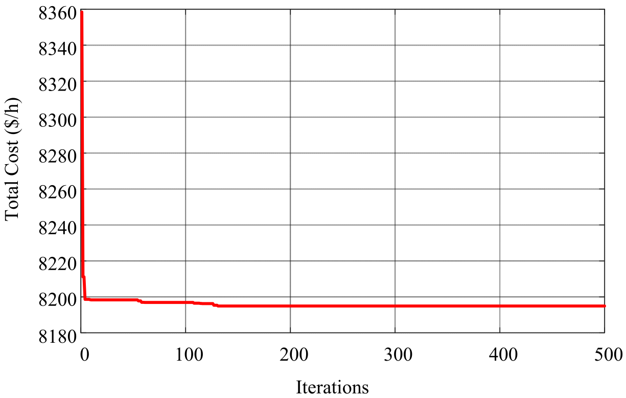
The convergence curve shows that the proposed FMPA rapidly reduces the total fuel cost during the early iterations, indicating strong exploration capability at the beginning of the search process as shown in Figure 1. Afterward, the cost gradually stabilizes around the best solution, showing that the algorithm efficiently shifts toward exploitation and reaches convergence without large oscillations. The nearly flat curve after the initial stage confirms the stable convergence behavior of FMPA for the 3-unit ELD system.

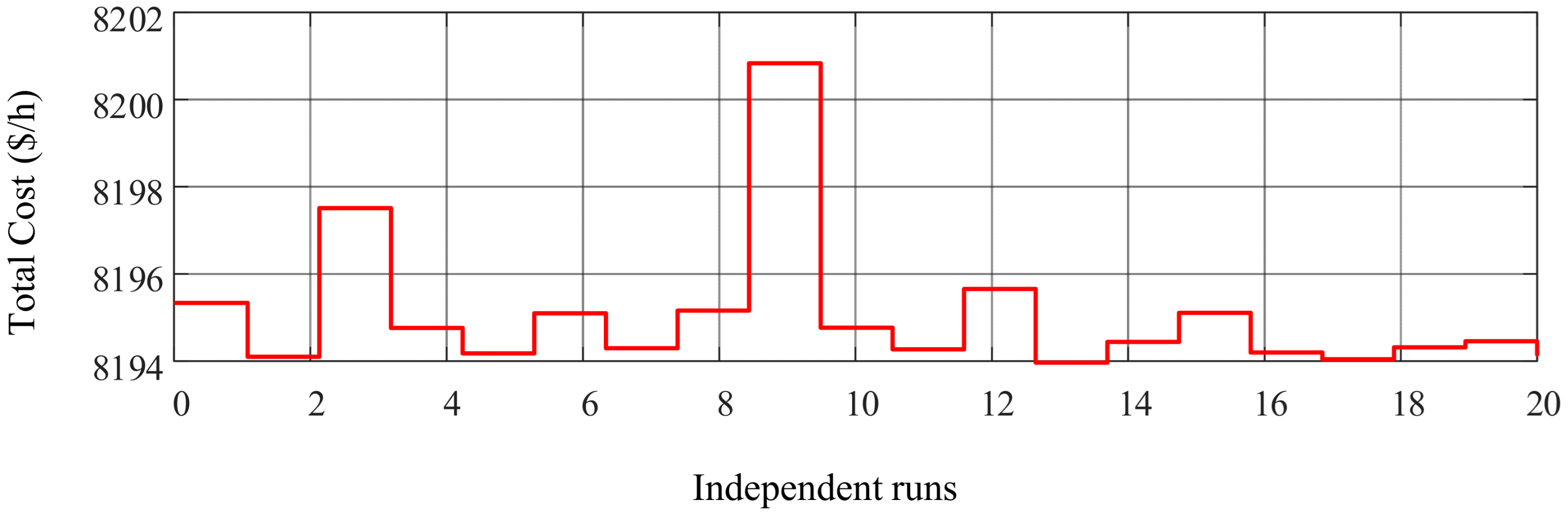
Figure 2 presents the fuel cost obtained over 20 independent runs. The results remain within a narrow cost range, mostly close to the best value, which demonstrates the repeatability and robustness of the proposed method. Although a few runs show slightly higher costs, the overall variation is small, confirming that FMPA can consistently generate high-quality solutions under different random starting conditions.

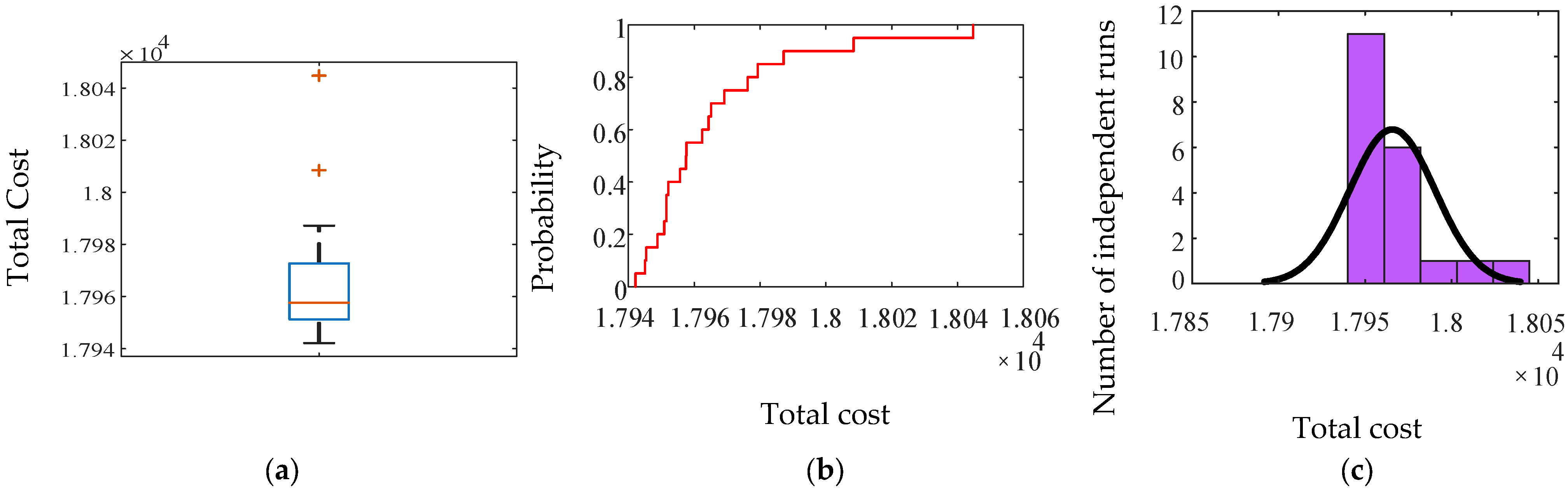
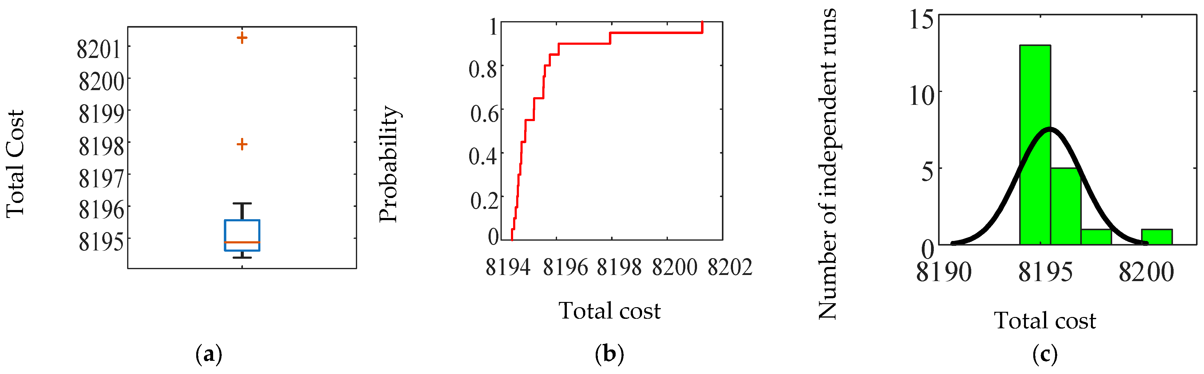
The statistical plots further validate the performance of FMPA, as shown in Figure 3. The boxplot shows a compact distribution with a small interquartile range, indicating low variability among the obtained costs as illustrated in Figure 3a. The CDF curve rises sharply, showing that most independent runs achieve costs near the minimum value as depicted in Figure 3b. Similarly, the histogram confirms that most solutions are concentrated around the optimal cost region, with only a few scattered higher-cost observations as shown in Figure 3c. Overall, these statistical results verify the stability, reliability, and robustness of the proposed FMPA.

4.2. Thirteen Thermal Unit Test System

This case study evaluates the performance of the proposed FMPA on a 13-unit thermal generation system with a total load demand of 1800 MW. The generator operating limits and cost coefficients are adopted from well-established benchmark datasets available in the literature [10,15,30,52,57]. The obtained results are presented in

Table 3. Comparative optimal generation results of the proposed FMPA and existing optimization techniques for the 13-unit ELD system.

Generating Units	FGOA-SQP [2]	GWO [10]	QOPO [52]	NN-EPSO [10]	MFO [29]	MMFO [29]	QOPO [52]	FMPA
1	506.9118	807.1247	628.3183	490	807.1247	481.7726	628.3183	555.8775
2	253.4559	144.869	298.1864	189	144.869	194.1905	298.1864	268.8090
3	253.4559	297.9434	223.7622	214	297.9434	244.7307	223.7622	221.6221
4	99.3628	60	60.00008	160	60	116.1982	60.00008	86.2895
5	99.3628	60	60	90	60	117.4941	60	88.1261
6	99.3627	60	60	120	60	132.1647	60	94.1338
7	99.3627	60	159.7331	103	60	77.94045	159.7331	121.3920
8	99.3628	60	60	88	60	125.2659	60	113.7500
9	99.3627	60.0362	60	104	60.0362	92.16435	60	60
10	40.0000	40	40	13	40	40	40	40
11	40.0000	40.0267	40	58	40.0267	43.26936	40	40
12	55.0000	55	55	66	55	78.6438	55	55
13	55.0000	55	55.00001	55	55	56.16537	55.0001	55
Total Cost (USD/h)	17,932.4741	18,051.11	17,988.99	18,442.59	18,008.89	17,960.14	17,988.99	17,942.1594

and compared with several existing optimization techniques, including GWO, QOPO, NN-EPSO, MFO, and MMFO. The results show that the proposed FMPA attains a competitive and optimal generation cost of 17,942.1594 USD/h, outperforming most compared methods. The optimal power distribution across all generating units satisfies the load demand while maintaining cost efficiency. Compared to existing techniques, the proposed method shows competitive and consistent improvement in minimizing fuel cost, particularly in handling the nonlinear characteristics of the ELD problem.

For the 13-unit test system, the statistical indicators in

Table 4. Statistical performance of the proposed FMPA over 20 independent runs for the 13-unit ELD system.

Test System	Best Cost (USD/h)	Median (USD/h)	Mean Cost (USD/h)	Worst Cost (USD/h)	Std. Dev. (USD/h)
13-unit system	17,942.1594	17,956.8638	17,967.8099	18,046.2876	29.9676

show that FMPA maintains reliable performance under increased problem dimensionality, achieving a best cost of 17,942.1594USD/h and a standard deviation of 29.9676 USD/h across 20 independent runs. This limited variation confirms that the algorithm can preserve convergence stability while handling a larger search space. The comparative analysis demonstrates that FMPA delivers cost benefits between about 0.10% and 2.71% higher than other applied optimization algorithms.

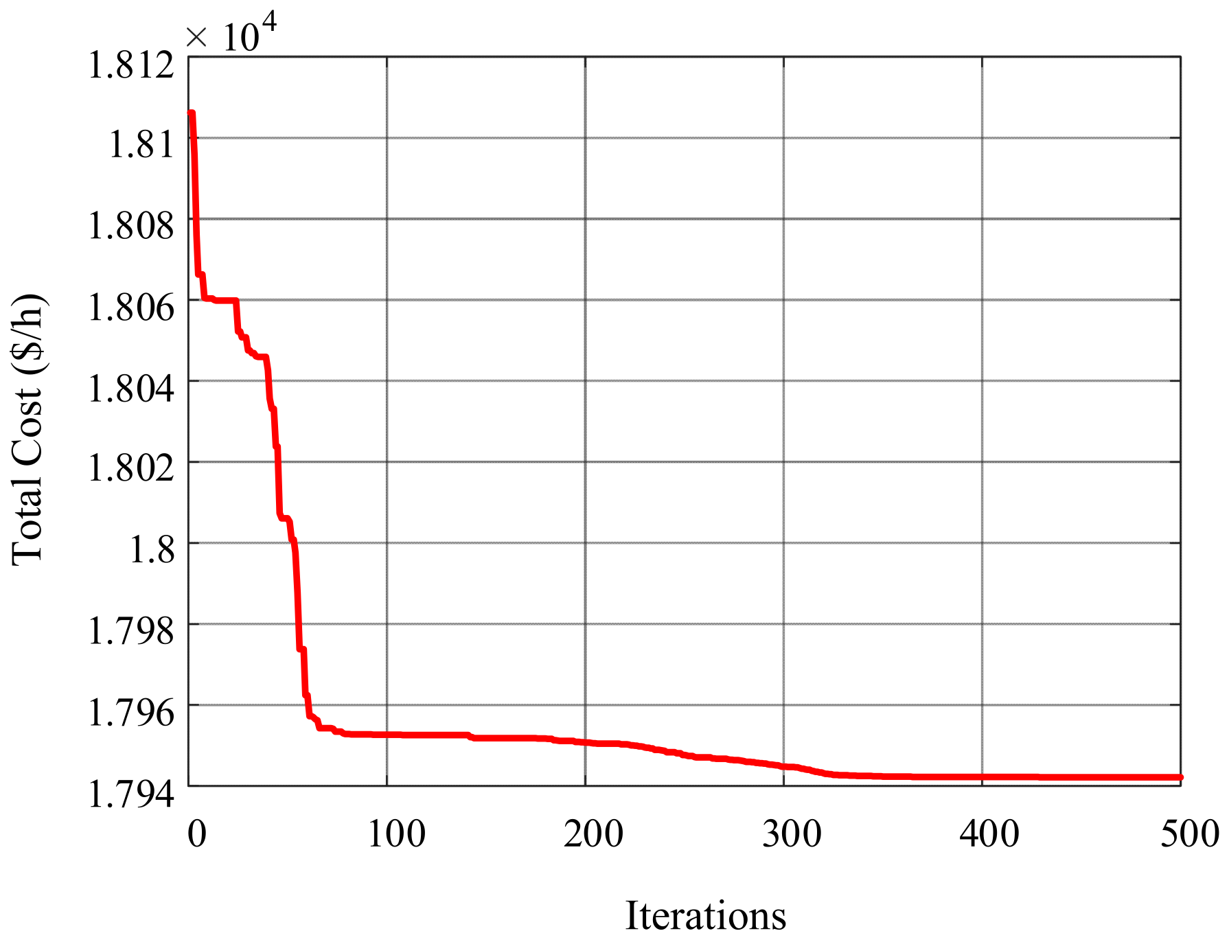
The largest improvements are achieved over NN-EPSO. While modest, meaningful gains are observed relative to GWO, MFO, and MMFO. Even small reductions in generation cost yield significant economic benefits in large-scale power systems. This proves that the developed FMPA algorithm not only produces better-quality solutions, but also scales effectively for medium-size ELD problems and surpasses several state-of-the-art optimization techniques. From the convergence curve of the 13-unit thermal system shown in Figure 4, it is observed that the proposed method achieves rapid cost reduction in the early iterations and reaches the optimal value within a few iterations.

The independent run test result also proves the stability of the suggested FMPA method illustrated in Figure 5. Despite slight differences in each of the 20 runs because of different starting positions, the results still converge on the region of minimum cost, indicating the reliability of the method for high dimensional problems.

The statistical analysis offers further information about the quality of the solutions, as depicted in Figure 6. The box plot depicts a tight distribution pattern with narrow variation, whereas the cumulative distribution function demonstrates that a considerable number of iterations tend toward the optimal solution. The histogram reveals a strong concentration of results around the optimal cost, with very few deviations. These observations collectively confirm that FMPA maintains stability, consistency, and robustness when applied to medium-scale ELD problems.

4.3. Thirty-Seven Thermal and Three Wind Power Units

This case study analyzes the performance of the proposed FMPA on a large-scale ELD dispatch system consisting of 40 generating units, including 37 thermal units and 3 wind power sources. The system parameters are adopted from widely accepted benchmark datasets to ensure fair comparison [24,30,56,57,58]. The optimal generation schedule for a total demand of 10,500 MW is presented in

Table 5. Comparative optimal generation results of the proposed FMPA and existing optimization techniques for the 40-unit ELD system.

Power Units	FGOA-SQP [4]	FWOA- I [5]	FWOA-II [5]	FWOA-III [5]	FWOA-IV [5]	MFO [29]	MMFO [29]	FMPA
1	36.0000	114	114	114	114	114	112.2146	36
2	114.0000	114	114	114	114	110.782043	85.7714	114
3	97.4002	120	60	120	120	97.35768193	88.2117	60
4	190.0000	80	190	190	190	179.853732	180.9641	190
5	97.0000	97	97	97	97	47	82.4790	87.7999
6	68.0000	140	140	140	140	140	139.9986	140
7	259.6000	300	300	300	300	300	300	259.5908
8	300.0000	300	300	300	300	300	289.7228	300
9	300.0000	300	300	300	284	285.1041	288.4185	300
10	130.0000	130	130	130	130	130	200.5044	130
11	94.0000	94	94	94	94	318.0878	289.2551	94
12	94.0000	94	94	94	94	94	243.7934	313.9730
13	394.2788	125	125	125	125	216.8874	304.4608	125
14	394.2789	393	321	305	125	484.0405941	390.7212	500
15	484.0380	394	218	300	215	500	500	500
16	304.5192	125	301	125	500	500	353.3224	394.2649
17	489.2799	500	500	500	500	500	313.0460	500
18	500.0000	500	500	500	500	220	421.2108	220
19	421.5199	550	550	550	550	511.4687	495.8544	331.7598
20	511.2795	550	550	550	504	550	518.3697	550
21	523.2804	550	550	550	550	523.2265	534.9080	550
22	523.2801	550	550	550	549	345.1678	519.7360	550
23	523.2798	550	550	550	550	523.2798	461.0149	550
24	523.2799	550	550	550	550	550	532.9676	550
25	523.2800	550	550	550	542	523.2365	532.8027	523.2792
26	523.2799	550	522	550	550	522.6056	541.2884	550
27	47.0000	97	87	97	97	47	80.9368	87.7999
28	190.0000	190	190	190	190	163.3979	112.6556	159.7331
29	190.0000	190	190	190	190	169.6291	126.9149	190
30	159.7338	190	190	190	190	190	158.8551	190
31	200.0000	200	200	200	198	172.465	199.9890	90
32	200.0000	200	200	200	198	166.535	172.3346	164.7995
33	164.8002	200	200	200	166	90	90	200
34	89.1143	25	110	110	110	65.63347	86.84495	110
35	110.0000	110	110	110	96	110	57.10207	110
36	101.1978	110	85	110	110	110	72.98398	110
37	511.2794	550	550	537	550	511.2403	500.4913	550
38	18.0000	18	18	18	18	18	19.85508	18
39	46.0000	46	46	46	46	46	46.0001	46
40	54.0000	54	54	54	54	54	54	54
Total Cost	137,208.4176	149,598.9	145,750.4	142,413.4	141,195.7	139,576.3965	138,155.7853	138,256.24

, along with comparisons against several established optimization methods. The statistical evaluation of FMPA over 20 independent runs for the considered case study is presented in

Table 6. Statistical performance of the proposed FMPA over 20 independent runs for the 40-unit ELD system.

Test System	Best Cost (USD/h)	Mediant Cost (USD/h)	Mean Cost (USD/h)	Worst Cost (USD/h)	Std. Dev. (USD/h)
40-unit system	138,256.24	140,958.9116	141,837.4404	151,523.1025	3299.8778

.

Table 7. Comparative analysis of minimum fuel cost for the 40-unit ELD system using different optimization techniques.

Optimization Techniques	Minimum Fuel Cost
FGOA-SQP [4]	137,208.4176
Best Compromise [58]	143,587.90
GAEPSO [24]	146,035.00
PWTED2 [10]	156,878.97
COOT [30]	139,000.63
FWOA-I [5]	149,598.9
EMA [10]	144,356.00
FWOA-IV [5]	141,195.7
PSO [24]	142,068.00
DWTED2 [58]	154,993.00
FWOA-III [5]	142,413.4
MFO [29]	139,576.3965
FWOA-II [5]	145,750.4
FMPA	138,256.24

summarizes the total operating cost obtained by each technique. The results show that the proposed FMPA achieves a total generation cost of 138,256.24 USD/h, which is highly competitive with existing approaches. Although a marginal difference is observed compared to the best-performing method, the proposed algorithm consistently delivers near-optimal solutions. When compared to other approaches, including FWOA versions, the proposed approach shows significant reductions in costs, indicating its efficacy in solving complex and large-scale ELD problems. Specifically, the proposed FMPA provides cost reductions ranging between 7% and 8%, which is significantly higher than that obtained by other algorithms, such as FWOA-I, without sacrificing performance by only 0.1%. Moreover, when compared to various optimization algorithms, the proposed FMPA provides cost reductions ranging between 0.5% and 11.8%.

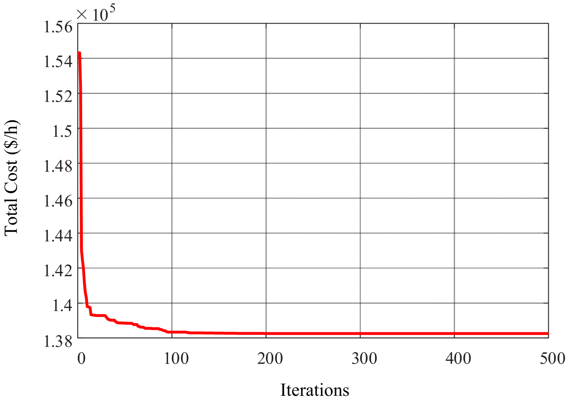
The obtained results support that the developed methodology yields solutions of high quality at reduced cost while retaining consistent convergence properties, as illustrated in Figure 7. The ability to maintain consistent performance even in such a large-scale environment is evidence of the strength and scalability of the algorithm, capable of generating reliable solutions to the ELD problem.

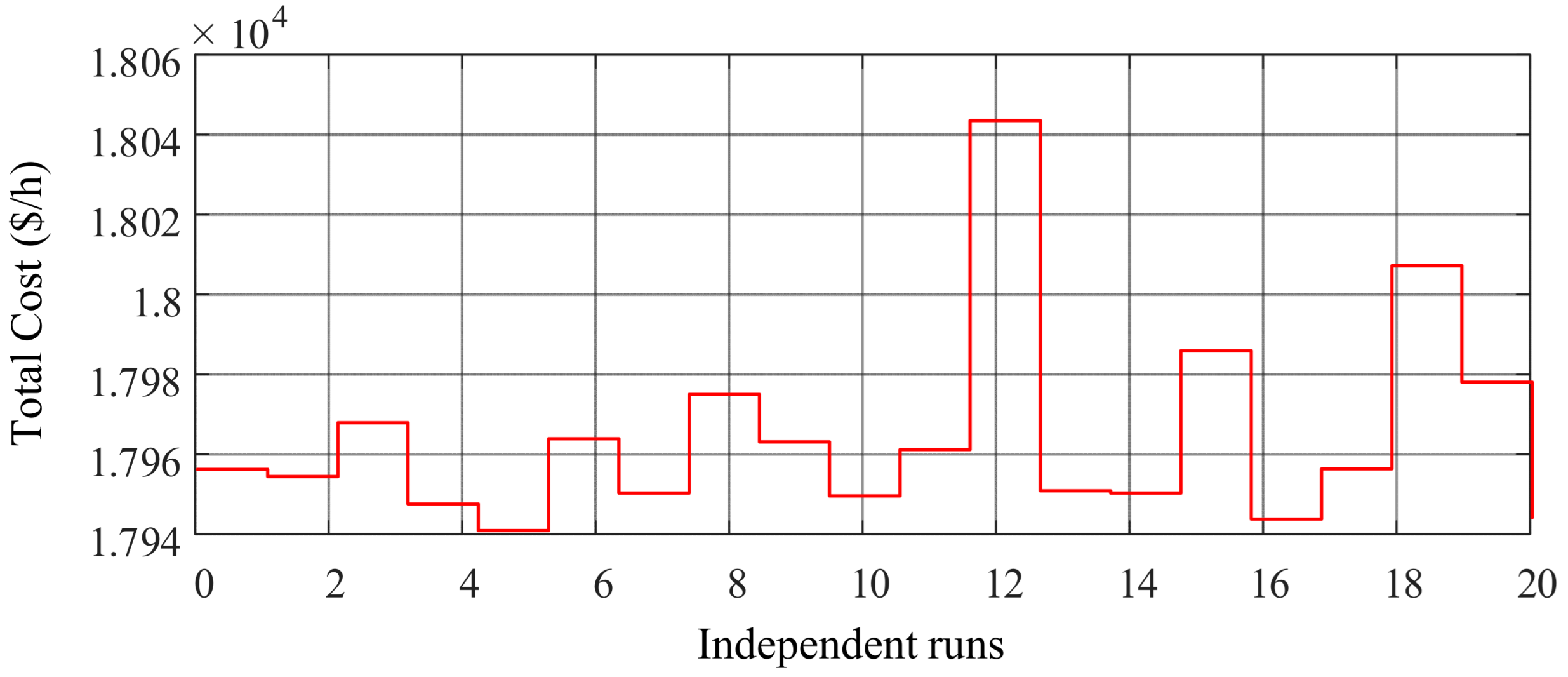
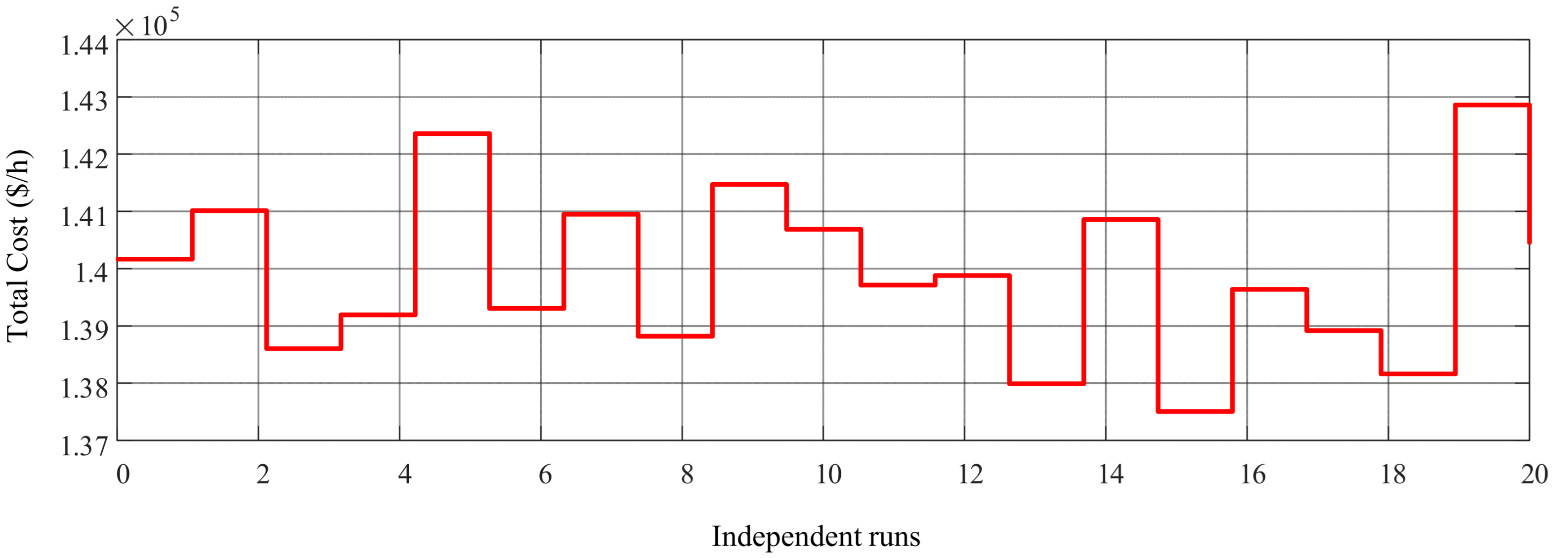
Figure 8 illustrates the total generation cost obtained by the proposed FMPA over 20 independent runs for the 40-unit system. Each data point corresponds to a separate execution initialized with different random conditions. The narrow variation in cost values indicates that the algorithm consistently converges to high-quality solutions despite changes in initial population. The limited dispersion of results demonstrates the robustness and stability of the proposed method when applied to large-scale ELD problems.

For the 40-unit system, the statistical results indicate that FMPA remains effective under large-scale and wind-integrated operating conditions, achieving a best cost of 138,256.24 USD/h with a standard deviation of 3299.8778 USD/h across 20 runs, as shown in Table 6. Although the variation is higher than in smaller systems due to increased dimensionality and renewable uncertainty, the results remain concentrated around a competitive cost region, confirming the scalability of the proposed method.

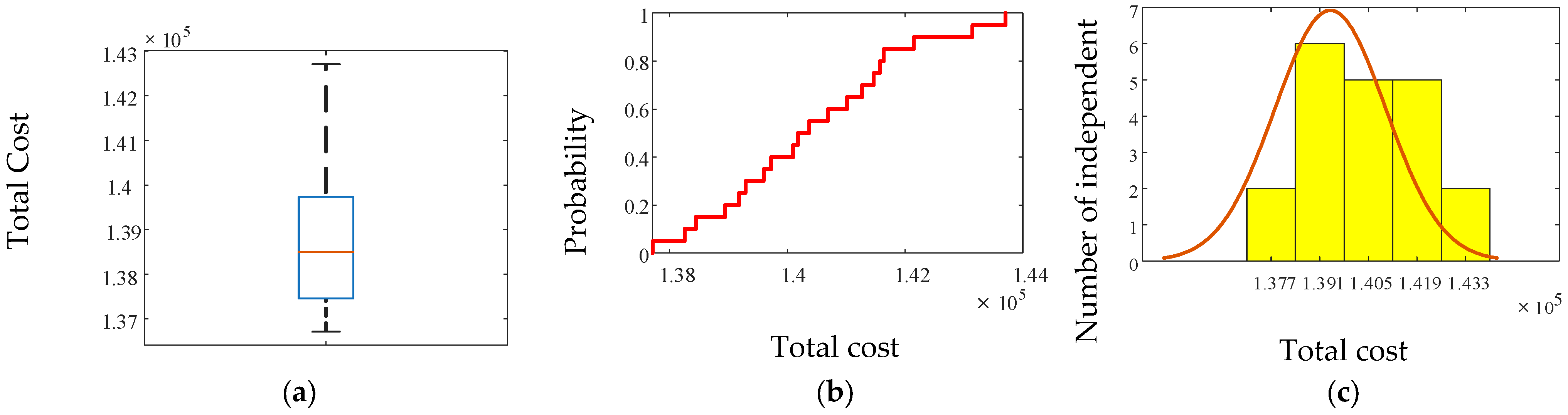
The statistical analysis for the 40-unit system highlights the consistency and reliability of the proposed FMPA under large-scale conditions, as shown in Figure 9. The boxplot indicates a reasonably compact distribution with limited outliers, reflecting stable performance despite increased problem complexity. The CDF shows that most runs converge within a narrow cost range close to the optimal value, while the histogram exhibits a concentrated distribution around the mean cost. Overall, these results confirm that FMPA maintains robust and repeatable performance, demonstrating its scalability and effectiveness for high-dimensional ELD problems.

5. Conclusions

This study presented a FMPA for solving the ELD problem under nonlinear and uncertain operating conditions. By incorporating fractional calculus into the conventional MPA, the proposed method introduces a memory-driven search mechanism that improves the balance between exploration and exploitation, resulting in smoother convergence and enhanced solution stability. The effectiveness of FMPA was evaluated using benchmark ELD systems of different scales, including 3-unit and 13-unit thermal systems, as well as 40-unit wind-integrated system. The results show that FMPA provides competitive and near-optimal fuel cost solutions compared with several established optimization techniques. For the smaller test system, the proposed method achieved results with negligible deviation from the best reported values, while for the medium- and large-scale systems, it demonstrated reliable scalability and robust convergence behavior. The statistical analysis over 20 independent runs further confirmed the consistency of the proposed algorithm. The low standard deviation for the 3-unit and 13-unit systems indicates stable repeatability, while the 40-unit ELD test system results demonstrate that FMPA can maintain competitive performance even under increased dimensionality and renewable energy uncertainty. Overall, the proposed FMPA offers an efficient and scalable optimization framework for nonlinear, nonconvex, and high-dimensional ELD problems. Future work may extend the approach to multi-objective dispatch, real-time optimization, and hybrid renewable energy systems.

References

1. Secui, D.C.; Hora, C.; Dan, F.C.; Secui, M.L.; Hora, H.N.; Gligor, E. A social group optimization algorithm using the laplace operator for the economic dispatch problem. Processes 2025, 13, 405. [Google Scholar] [CrossRef]
2. Kumar, P.; Ali, M. Solving the economic load dispatch problem by attaining and refining knowledge-based optimization. Mathematics 2025, 13, 1042. [Google Scholar] [CrossRef]
3. Cadena-Albuja, J.; Barrera-Singaña, C.; Arcos, H.; Muñoz, J. Economic Dispatch in Electrical Systems with Hybrid Generation Using the Differential Evolution Algorithm: A Comparative Analysis with Other Optimization Techniques Under Energy Limitation Scenarios. Energies 2025, 18, 3414. [Google Scholar] [CrossRef]
4. Wadood, A.; Khan, B.S.; Khan, B.M.; Park, H.; Kang, B.O. A Fractional Hybrid Strategy for Reliable and Cost-Optimal Economic Dispatch in Wind-Integrated Power Systems. Fractal Fract. 2026, 10, 64. [Google Scholar] [CrossRef]
5. Wadood, A.; Sattar Khan, B.; Albalawi, H.; Alatwi, A.M. Design of the novel fractional order hybrid whale optimizer for thermal wind power generation systems with integration of chaos infused wind power. Fractal Fract. 2024, 8, 379. [Google Scholar] [CrossRef]
6. Labbi, Y.; Attous, D.B.; Mahdad, B. Artificial bee colony optimization for economic dispatch with valve point effect. Front. Energy 2014, 8, 449–458. [Google Scholar] [CrossRef]
7. Labbi, Y.; Attous, D.B. A Hybrid Big Bang–Big Crunch optimization algorithm for solving the different economic load dispatch problems. Int. J. Syst. Assur. Eng. Manag. 2017, 8, 275–286. [Google Scholar] [CrossRef]
8. Labbi, Y.; Attous, D.B. A hybrid particle swarm optimization and pattern search method to solve the economic load dispatch problem. Int. J. Syst. Assur. Eng. Manag. 2014, 5, 435–443. [Google Scholar] [CrossRef]
9. Kamboj, V.K.; Bhadoria, A.; Bath, S.K. Solution of non-convex economic load dispatch problem for small-scale power systems using ant lion optimizer. Neural Comput. Appl. 2017, 28, 2181–2192. [Google Scholar] [CrossRef]
10. Kamboj, V.K.; Bath, S.K.; Dhillon, J.S. Solution of non-convex economic load dispatch problem using Grey Wolf Optimizer. Neural Comput. Appl. 2016, 27, 1301–1316. [Google Scholar] [CrossRef]
11. Jayabarathi, T.; Yazdani, A.; Ramesh, V. Application of the invasive weed optimization algorithm to economic dispatch problems. Front. Energy 2012, 6, 255–259. [Google Scholar] [CrossRef]
12. Jayabarathi, T.; Bahl, P.; Ohri, H.; Yazdani, A.; Ramesh, V. A hybrid BFA-PSO algorithm for economic dispatch with valve-point effects. Front. Energy 2012, 6, 155–163. [Google Scholar] [CrossRef]
13. Jain, N.K.; Nangia, U.; Jain, J. Economic load dispatch using adaptive social acceleration constant based particle swarm optimization. J. Inst. Eng. (India) Ser. B 2018, 99, 431–439. [Google Scholar] [CrossRef]
14. Jain, N.K.; Nangia, U.; Jain, A. PSO for multiobjective economic load dispatch (MELD) for minimizing generation cost and transmission losses. J. Inst. Eng. (India) Ser. B 2016, 97, 185–191. [Google Scholar] [CrossRef]
15. Hsieh, Y.Z.; Su, M.C. AQ-learning-based swarm optimization algorithm for economic dispatch problem. Neural Comput. Appl. 2016, 27, 2333–2350. [Google Scholar] [CrossRef]
16. Said, M.; El-Rifaie, A.M.; Tolba, M.A.; Houssein, E.H.; Deb, S. An efficient chameleon swarm algorithm for economic load dispatch problem. Mathematics 2021, 9, 2770. [Google Scholar] [CrossRef]
17. Ramalingam, R.; Karunanidy, D.; Alshamrani, S.S.; Rashid, M.; Mathumohan, S.; Dumka, A. Oppositional pigeon-inspired optimizer for solving the non-convex economic load dispatch problem in power systems. Mathematics 2022, 10, 3315. [Google Scholar] [CrossRef]
18. Yu, X.; Yu, X.; Lu, Y.; Sheng, J. Economic and emission dispatch using ensemble multi-objective differential evolution algorithm. Sustainability 2018, 10, 418. [Google Scholar] [CrossRef]
19. Prakash, T.; Singh, V.P.; Singh, S.P.; Mohanty, S.R. Economic load dispatch problem: Quasi-oppositional self-learning TLBO algorithm. Energy Syst. 2018, 9, 415–438. [Google Scholar] [CrossRef]
20. Pattanaik, J.K.; Basu, M.; Dash, D.P. Dynamic economic dispatch: A comparative study for differential evolution, particle swarm optimization, evolutionary programming, genetic algorithm, and simulated annealing. J. Electr. Syst. Inf. Technol. 2019, 6, 1. [Google Scholar] [CrossRef]
21. Nascimento, M.H.R.; Nunes, M.V.A.; Rodríguez, J.L.M.; Leite, J.C. A new solution to the economical load dispatch of power plants and optimization using differential evolution. Electr. Eng. 2017, 99, 561–571. [Google Scholar] [CrossRef]
22. Murali, K.; Jayabarathi, T. Solution to economic dispatch problem with valve-point loading effect by using catfish PSO algorithm. Front. Energy 2014, 8, 290–296. [Google Scholar] [CrossRef]
23. Mahdad, B.; Srairi, K. Solving practical economic dispatch using hybrid GA–DE–PS method. Int. J. Syst. Assur. Eng. Manag. 2014, 5, 391–398. [Google Scholar] [CrossRef]
24. Hagh, M.T.; Kalajahi, S.M.S.; Ghorbani, N. Solution to economic emission dispatch problem including wind farms using Exchange Market Algorithm Method. Appl. Soft Comput. 2020, 88, 106044. [Google Scholar] [CrossRef]
25. Morshed, M.J.; Asgharpour, A. Hybrid imperialist competitive-sequential quadratic programming (HIC-SQP) algorithm for solving economic load dispatch with incorporating stochastic wind power: A comparative study on heuristic optimization techniques. Energy Convers. Manag. 2014, 84, 30–40. [Google Scholar] [CrossRef]
26. Pandit, M.; Chaudhary, V.; Dubey, H.M.; Panigrahi, B.K. Multi-period wind integrated optimal dispatch using series PSO-DE with time-varying Gaussian membership function based fuzzy selection. Int. J. Electr. Power Energy Syst. 2015, 73, 259–272. [Google Scholar] [CrossRef]
27. Jiang, S.; Ji, Z.; Wang, Y. A novel gravitational acceleration enhanced particle swarm optimization algorithm for wind–thermal economic emission dispatch problem considering wind power availability. Int. J. Electr. Power Energy Syst. 2015, 73, 1035–1050. [Google Scholar] [CrossRef]
28. Wadood, A.; Khan, B.S.; Khurshaid, T.; Kim, K.C.; Rhee, S.B. Chaos-infused wind power integration in the grey wolf optimal paradigm for combine thermal-wind power plant systems. Front. Energy Res. 2024, 12, 1301700. [Google Scholar] [CrossRef]
29. Albalawi, H.; Wadood, A.; Park, H. Economic load dispatch problem analysis based on modified moth flame optimizer (MMFO) considering emission and wind power. Mathematics 2024, 12, 3326. [Google Scholar] [CrossRef]
30. Khan, B.S.; Qamar, A.; Wadood, A.; Almuhanna, K.; Al-Shamma, A.A. Integrating economic load dispatch information into the blockchain smart contracts based on the fractional-order swarming optimizer. Front. Energy Res. 2024, 12, 1350076. [Google Scholar] [CrossRef]
31. Khan, B.S.; Raja, M.A.Z.; Qamar, A.; Chaudhary, N.I. Design of moth flame optimization heuristics for integrated power plant system containing stochastic wind. Appl. Soft Comput. 2021, 104, 107193. [Google Scholar] [CrossRef]
32. Ali, T.; Yasin, S.; Draz, U.; Samkari, H.S.; Hijji, M.; Allehyani, M.F.; Wadood, A. Fractional-Order Dynamic Modeling of Renewable-Dominant Power Systems Using Long-Memory Load and Generation Data. Fractal Fract. 2026, 10, 183. [Google Scholar] [CrossRef]
33. Ali, T.; Muhammad, A.; Samkari, H.S.; Mohammad, H.; Allehyani, M.F. Multi-Objective Optimization and Load-Flow Analysis in Complex Power Distribution Networks. Fractal Fract. 2026, 10, 82. [Google Scholar] [CrossRef]
34. Ghamisi, P.; Couceiro, M.S.; Benediktsson, J.A. A novel feature selection approach based on FODPSO and SVM. IEEE Trans. Geosci. Remote Sens. 2014, 53, 2935–2947. [Google Scholar] [CrossRef]
35. Ates, A.; Alagoz, B.B.; Kavuran, G.; Yeroglu, C. Implementation of fractional order filters discretized by modified fractional order darwinian particle swarm optimization. Measurement 2017, 107, 153–164. [Google Scholar] [CrossRef]
36. Couceiro, M.S.; Rocha, R.P.; Ferreira, N.F.; Machado, J.T. Introducing the fractional-order Darwinian PSO. Signal Image Video Process. 2012, 6, 343–350. [Google Scholar] [CrossRef]
37. Shahri, E.S.A.; Alfi, A.; Machado, J.T. Fractional fixed-structure H∞ controller design using augmented Lagrangian particle swarm optimization with fractional order velocity. Appl. Soft Comput. 2019, 77, 688–695. [Google Scholar] [CrossRef]
38. Machado, J.T.; Kiryakova, V. The chronicles of fractional calculus. Fract. Calc. Appl. Anal. 2017, 20, 307–336. [Google Scholar] [CrossRef]
39. Kuttomparambil Abdulkhader, H.; Jacob, J.; Mathew, A.T. Fractional-order lead-lag compensator-based multi-band power system stabiliser design using a hybrid dynamic GA-PSO algorithm. IET Gener. Transm. Distrib. 2018, 12, 3248–3260. [Google Scholar] [CrossRef]
40. Kosari, M.; Teshnehlab, M. Non-linear fractional-order chaotic systems identification with approximated fractional-order derivative based on a hybrid particle swarm optimization-genetic algorithm method. J. AI Data Min. 2018, 6, 365–373. [Google Scholar]
41. Wadood, A.; Park, H. A novel application of fractional order derivative moth flame optimization algorithm for solving the problem of optimal coordination of directional overcurrent relays. Fractal Fract. 2024, 8, 251. [Google Scholar] [CrossRef]
42. Wadood, A.; Ahmed, E.; Rhee, S.B.; Sattar Khan, B. A Fractional-Order Archimedean Spiral Moth–Flame Optimization Strategy to Solve Optimal Power Flows. Fractal Fract. 2024, 8, 225. [Google Scholar] [CrossRef]
43. Qu, B.Y.; Zhu, Y.S.; Jiao, Y.C.; Wu, M.Y.; Suganthan, P.N.; Liang, J.J. A survey on multi-objective evolutionary algorithms for the solution of the environmental/economic dispatch problems. Swarm Evol. Comput. 2018, 38, 1–11. [Google Scholar] [CrossRef]
44. Sheta, A.; Faris, H.; Braik, M.; Mirjalili, S. Nature-inspired metaheuristics search algorithms for solving the economic load dispatch problem of power system: A comparison study. In Applied Nature-Inspired Computing: Algorithms and Case Studies; Springer: Singapore, 2019; pp. 199–230. [Google Scholar]
45. Faramarzi, A.; Heidarinejad, M.; Mirjalili, S.; Gandomi, A.H. Marine Predators Algorithm: A nature-inspired metaheuristic. Expert Syst. Appl. 2020, 152, 113377. [Google Scholar] [CrossRef]
46. Einstein, A. Investigations on the Theory of the Brownian Movement; Courier Corporation: North Chelmsford, MA, USA, 1956; ISBN 9780486603049. [Google Scholar]
47. Mantegna, R.N. Fast, accurate algorithm for numerical simulation of Levy stable stochastic processes. Phys. Rev. E 1994, 49, 4677. [Google Scholar] [CrossRef] [PubMed]
48. Filmalter, J.D.; Dagorn, L.; Cowley, P.D.; Taquet, M. First descriptions of the behavior of silky sharks, Carcharhinus falciformis, around drifting fish aggregating devices in the Indian Ocean. Bull. Mar. Sci. 2011, 87, 325–337. [Google Scholar] [CrossRef]
49. Teodoro, G.S.; Machado, J.T.; De Oliveira, E.C. A review of definitions of fractional derivatives and other operators. J. Comput. Phys. 2019, 388, 195–208. [Google Scholar] [CrossRef]
50. Sabatier, J.A.T.M.J.; Agrawal, O.P.; Machado, J.T. Advances in Fractional Calculus; Springer: Dordrecht, The Netherlands, 2007; Volume 4. [Google Scholar]
51. Basetti, V.; Rangarajan, S.S.; Shiva, C.K.; Pulluri, H.; Kumar, R.; Collins, R.E.; Senjyu, T. Economic emission load dispatch problem with valve-point loading using a novel quasi-oppositional-based political optimizer. Electronics 2021, 10, 2596. [Google Scholar] [CrossRef]
52. Alsumait, J.S.; Sykulski, J.K.; Al-Othman, A.K. A hybrid GA–PS–SQP method to solve power system valve-point economic dispatch problems. Appl. Energy 2010, 87, 1773–1781. [Google Scholar] [CrossRef]
53. Duman, S.; Güvenç, U.; Yörükeren, N. Gravitational search algorithm for economic dispatch with valve-point effects. Int. Rev. Electr. Eng. 2010, 5, 2890–2895. [Google Scholar]
54. Cai, J.; Li, Q.; Li, L.; Peng, H.; Yang, Y. A hybrid CPSO–SQP method for economic dispatch considering the valve-point effects. Energy Convers. Manag. 2012, 53, 175–181. [Google Scholar] [CrossRef]
55. Tsai, M.T.; Gow, H.J.; Lin, W.M. A novel stochastic search method for the solution of economic dispatch problems with non-convex fuel cost functions. Int. J. Electr. Power Energy Syst. 2011, 33, 1070–1076. [Google Scholar] [CrossRef]
56. Sinha, N.; Chakrabarti, R.; Chattopadhyay, P.K. Evolutionary programming techniques for economic load dispatch. IEEE Trans. Evol. Comput. 2003, 7, 83–94. [Google Scholar] [CrossRef]
57. Victoire, T.A.A.; Jeyakumar, A.E. Hybrid PSO–SQP for economic dispatch with valve-point effect. Electr. Power Syst. Res. 2004, 71, 51–59. [Google Scholar] [CrossRef]
58. Azizipanah-Abarghooee, R.; Niknam, T.; Roosta, A.; Malekpour, A.R.; Zare, M. Probabilistic multiobjective wind-thermal economic emission dispatch based on point estimated method. Energy 2012, 37, 322–335. [Google Scholar] [CrossRef]
Figure 1. Convergence characteristics of the proposed FMPA for the 3-unit ELD system.
Fractalfract 10 00363 g001
Figure 2. Total generation cost over 20 independent runs using FMPA for the 3-unit ELD system.
Fractalfract 10 00363 g002
Figure 3. Statistical performance of FMPA for the 3-unit ELD system using (a) boxplot, (b) CDF, and (c) histogram.
Fractalfract 10 00363 g003
Figure 4. Convergence characteristics of the proposed FMPA for the 13-unit ELD system.
Fractalfract 10 00363 g004
Figure 5. Total generation cost over 20 independent runs using FMPA for 13-unit ELD test system.
Fractalfract 10 00363 g005
Figure 6. Statistical performance of FMPA for the 13-unit ELD system using (a) boxplot, (b) CDF, and (c) histogram.
Fractalfract 10 00363 g006
Figure 7. Convergence characteristics of the proposed FMPA for the 40-unit ELD system.
Fractalfract 10 00363 g007
Figure 8. Total generation cost over 20 independent runs using FMPA for 40-unit ELD system.
Fractalfract 10 00363 g008
Figure 9. Statistical performance of FMPA for the 40-unit ELD system using (a) boxplot, (b) CDF, and (c) histogram.
Fractalfract 10 00363 g009